The planted directed polymer: inferring a random walk from noisy images

Sun Woo P. Kim swk34@cantab.ac.uk Department of Physics, King’s College London, Strand, London WC2R 2LS, United Kingdom    Austen Lamacraft TCM Group, Cavendish Laboratory, University of Cambridge, Cambridge CB3 0HE, United Kingdom
Abstract

We introduce and study the planted directed polymer, in which the path of a random walker is inferred from noisy ‘images’ accumulated at each timestep. Formulated as a nonlinear problem of Bayesian inference for a hidden Markov model, this problem is a generalisation of the directed polymer problem of statistical physics, coinciding with it in the limit of zero signal to noise. For a 1D walker we present numerical investigations and analytical arguments that no phase transition is present. When formulated on a Cayley tree, methods developed for the directed polymer are used to show that there is a transition with decreasing signal to noise where effective inference becomes impossible, meaning that the average fractional overlap between the inferred and true paths falls from one to zero.

I Introduction

Recent years have seen a great deal of research activity at the interface of statistical physics and Bayesian inference [1]. Broadly speaking, the connection is as follows. Suppose the system of interest is described by some random variables $\mathbf{x}$ following a prior probability distribution $p(\mathbf{x})$. We learn about $\mathbf{x}$ by measuring some other random variables $\mathbf{y}$, which are described by some conditional distribution or ‘measurement model’ $p(\mathbf{y}|\mathbf{x})$ 111Note that throughout we adopt the convention that different distributions are distinguished by the names of their arguments: a convenient abuse of notation. From the values of $\mathbf{y}$ we compute the posterior distribution $p(\mathbf{x}|\mathbf{y})$ of $\mathbf{x}$ using Bayes’ rule

$$p(\mathbf{x}|\mathbf{y})=\frac{p(\mathbf{y}|\mathbf{x})p(\mathbf{x})}{p(\mathbf{y})},$$ (1)

where the distribution of the measurement outcomes $p(\mathbf{y})=\sum_{\mathbf{x}}p(\mathbf{y}|\mathbf{x})p(\mathbf{x})$ can be regarded as a normalizing factor or partition function in the language of statistical physics. This setting is highly idealised, as it assumes for example perfect knowledge of the prior distribution and measurement model. Nevertheless, the computation of $p(\mathbf{x}|\mathbf{y})$ will in general be intractable when the number of variables $\mathbf{x}$ is large, due to the difficulty of calculating the denominator in Eq. 1. The intractability of the partition function is a general feature of statistical mechanical systems, and this represents the first point of contact between statistical physics and inference. Furthermore, there are ‘natural’ examples of inference problems over many variables where the phenomenology of phase transitions in the thermodynamic limit of random systems is applicable, with the values of the measurements $\mathbf{y}$ corresponding to the randomness. In the inference setting, such transitions represent a change in the structure of the posterior as a parameter representing the strength of the ‘signal’ of $\mathbf{x}$ in the measurements $\mathbf{y}$ is varied. As the signal weakens, the probability of successful inference goes to zero at the phase transition.

In this work, we will be concerned with developing the parallels between statistical mechanics and inference within a particular class of problems that have the structure of a hidden Markov model (HMM) (Fig. 1) [3, 4].

${\cdots}$ ${\mathbf{x}(t-1)}$ ${\mathbf{x}(t)}$ ${\mathbf{x}(t+1)}$ ${\cdots}$ ${\mathbf{y}(t-1)}$ ${\mathbf{y}(t)}$ ${\mathbf{y}(t+1)}$
Figure 1: Inference in a hidden Markov model

Here the prior $p(\mathbf{x})$ follows a Markov process

$\displaystyle p(x_{1:t})=\left(\prod_{\tau=2}^{t}p(x_{\tau}|x_{\tau-1})\right)p(x_{1}),$ (2)

where we have introduced the notation $x_{1:t}$ to denote a sequence of variables ${x_{1},\ldots x_{t}}$, and $p(x_{\tau}|x_{\tau-1})$ are the transition probabilities (or kernel) of the process. Measurements $y_{t}$ are conditional on the value $x_{t}$ at the same timestep through some measurement model $p(y_{t}|x_{t})$.

Inference in HMMs may involve one of several related tasks. Filtering refers to the problem of obtaining the posterior $p(x_{t}|y_{1:t})$ of the present value conditioned on the history of measurements, while smoothing involves conditioning additionally over future measurements. The most famous example of filtering in a HMM is the Kalman filter [5], in which both $p(x_{\tau}|x_{\tau-1})$ and $p(x_{t}|y_{t})$ are Gaussian with linear dependence on the conditioning variable. Because the product of Gaussians is also Gaussian, the filtering distribution $p(x_{t}|y_{1:t})$ — obtained from Bayes’ rule (1) — is a Gaussian with an explicit form.

Here we are concerned with a fundamentally nonlinear — though very natural — observation model, consisting of ‘images’ containing ‘pixels’, one for each possible state of the system $x$. Measurements $\phi_{x,t}$ are then indexed by both $x$ and $t$ and take the form

$\displaystyle\phi_{x,t}=\psi_{x,t}+\epsilon\delta_{x,x_{t}},$ (3)

where $\psi_{x,t}$ is Gaussian white noise and $\epsilon$ is a parameter that controls the relative strength of the signal (i.e. the signal-to-noise ratio). In Eq. 3 the shift of the mean of $\phi_{x_{t},t}$ by $\epsilon$ can reveal through which pixel the system has passed.

Problems of this type have appeared before in the engineering literature applied to tracking of paths through a noisy or cluttered environment [6, 7]. Our aim is to introduce and analyse a particularly simple version of the problem that we call the planted directed polymer problem, because of its connection with the statistical mechanics of a directed polymer in a random medium [8].

A second and quite different motivation for our work is the recently discovered measurement induced phase transition in monitored quantum systems, where the entanglement dynamics and purity of extensive quantum systems was found to undergo a transition in the long time limit as the measurement rate increases, see Refs. [9, 10] and the review Ref. [11]. While there is as of yet no formal connection between the phenomena explored here and those in the quantum setting, the resemblance between the two situations is suggestive.

Refer to caption
Figure 2: An example of Bayesian inference on a random walker from images with signal strength $\epsilon_{\mathrm{T}}=1.5$ and all other parameters $\sigma_{\mathrm{T}}=\sigma_{\mathrm{S}}=\epsilon_{\mathrm{S}}=1$. a) is a realisation of a random walker undergoing Brownian motion. b) shows the sets of ‘noisy images’ taken at each timestep. c) is the posterior distribution inferred from the noisy images.

The outline of the rest of this paper is as follows. In the next section we introduce the planted directed polymer problem and describe the relation to the directed polymer. In Sec. III we study the one dimensional case numerically to establish some general features of the phenomenology of the problem. In Sec. IV we present analytical results for the case of paths on a tree, building on the approach of Ref. [12] to the random polymer problem. Finally, we conclude in Sec. V and offer a perspective on similar problems in this class.

II Statement of the planted directed polymer problem

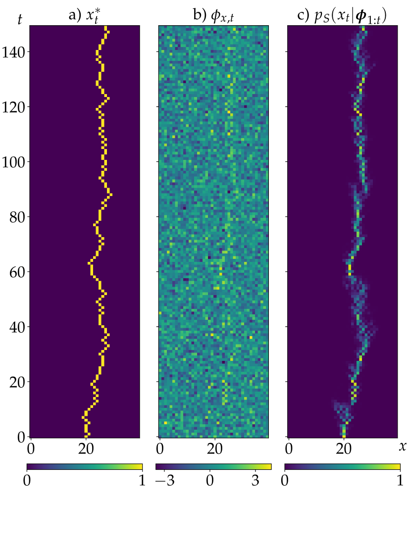
In this section we introduce the planted directed polymer problem. We describe the simplest case where the dynamics of our system is a random walk on the integers $\mathbb{Z}$: the generalisation to more complicated situations, including higher dimensions, should be obvious. The position of the walker at (integer) time $t$ is denoted by $x^{*}_{t}\in\mathbb{Z}$: throughout this work we follow Ref. [1] in using $x_{t}^{*}$ to denote the ‘ground truth’ or ‘planted’ configuration, with $x_{t}$ denoting the inferred configuration. The dynamics are specified by some transition kernel $p_{\mathrm{T}}(x^{*}_{t+1}|x^{*}_{t})$, with initial distribution $p_{\mathrm{T}}(x^{*}_{1})$ (the meaning of the subscript T will be explained shortly). As our main example we will take a symmetric random walk (see Fig. 2a)

$$p_{\mathrm{T}}(x^{*}_{t+1}|x^{*}_{t})=\frac{1}{2}\delta_{x^{*}_{t+1},x^{*}_{t}}+\frac{1}{4}\delta_{x^{*}_{t+1},x^{*}_{t}\pm 1}.$$ (4)

Our goal is to infer the walker’s trajectory from measurements that form noisy ‘images’ specified by a ‘pixel’ value $\phi_{x,t}$ at each position and time. These values are given by

$\displaystyle\phi_{x,t}=\psi_{x,t}+\epsilon_{\mathrm{T}}\delta_{x,x^{*}_{t}},$ (5)

where the pixel noise is a set of independent and identically distributed (iid) Gaussian distributions with standard deviation $\sigma_{\mathrm{T}}$, and $\epsilon_{\mathrm{T}}$ is the signal strength. An example is shown in Fig. 2b. We will sometimes use the standard probabilists’ notation $\mathcal{N}(\mu,\sigma^{2})$ for a normal distribution of mean $\mu$ and standard deviation $\sigma$, so that $\phi_{x,t}\sim p(\cdot|x^{*}_{t})=\mathcal{N}(\epsilon_{\mathrm{T}}\delta_{x_{t},x^{*}_{t}},\sigma_{\mathrm{T}}^{2})$. We use the bold symbol $\bm{\phi}_{t}:=(\phi_{x,t}|x\in\mathbb{Z})$ for the entire image at some time $t$. Following [1], we describe this process as the ‘teacher’, and indicate its parameters using the subscript T.

Given $\phi_{x,t}$, the ‘student’ can perform Bayesian inference to obtain the posterior over the walker’s trajectory $x_{1:t}$ given the past history of noisy images, $\bm{\phi}_{1:t}:=(\bm{\phi}_{\cdot,1},\dots,\bm{\phi}_{\cdot,t})$. We introduce the notation $X:=x_{1:t}$, $X^{*}:=x^{*}_{1:t}$ for the entire inferred and planted configurations respectively, and $\Phi:=\bm{\phi}_{1:t}$ for the sequence of images. The joint distribution is then

$\displaystyle p(X,\Phi,X^{*})=p_{\mathrm{S}}(X|\Phi)p_{\mathrm{T}}(\Phi|X^{*})p_{\mathrm{T}}(X^{*}).$ (6)

$p_{\mathrm{T}}(\Phi|X^{*})$ is the probability of obtaining the sequence of images conditioned on the path $X^{*}$, given by the above Gaussian distribution, and the student’s posterior over the path $X=x_{1:t}$ is given by Bayes’ rule

$\displaystyle p_{\mathrm{S}}(X|\Phi)=\frac{p_{\mathrm{S}}(\Phi|X)p_{\mathrm{S}}(X)}{\sum_{X^{\prime}}p_{\mathrm{S}}(\Phi|X^{\prime})p_{\mathrm{S}}(X^{\prime})}.$ (7)

We use the subscript S to denote the student’s distribution, which will allow us to consider a non Bayes-optimal setting in which the parameters of the student’s model do not coincide with those of the teacher. Later, we will also consider the case where the student also does not have access to the functional form of the teacher model. Eq. (6) defines the planted ensemble (in the terminology of Ref. [1]) for our problem.

Using the rules of conditional probability on the student’s prior we can also write the joint probability as

$\displaystyle p(X,\Phi,X^{*})=\frac{p_{\mathrm{S}}(\Phi|X)p_{\mathrm{S}}(X)p_{\mathrm{T}}(\Phi|X^{*})p_{\mathrm{T}}(X^{*})}{p_{\mathrm{S}}(\Phi)},$ (8)

where $p_{\mathrm{S}}(\Phi)=\sum_{X}p_{\mathrm{S}}(\Phi|X)p_{\mathrm{S}}(X)$. We see that in the Bayes optimal case, which is when the student and teacher distributions coincide, the joint distribution is symmetric with respect to $X\leftrightarrow X^{*}$. This means that inferred paths $X$ must have the same distribution as that of the true paths $X^{*}$.

Equation 6 represents a complete description of the problem, but dealing with the distribution over the entire trajectory is not normally practical. Instead, it is more usual to focus on the posterior distribution of the present value given the measurement history i.e. $p_{\mathrm{S}}(x_{t}|\bm{\phi}_{1:t})$ (the filtering problem). Below we present a tractable algorithm to calculate the posterior for the present value.

At $t=1$ Bayes’ rule gives

$\displaystyle p_{\mathrm{S}}(x_{1}|\bm{\phi}_{1})=\frac{p_{\mathrm{S}}(\bm{\phi}_{1}|x_{1})p_{\mathrm{S}}(x_{1})}{\sum_{x^{\prime}_{1}}p_{\mathrm{S}}(\bm{\phi}_{1}|x^{\prime}_{1})p_{\mathrm{S}}(x^{\prime}_{1})}.$ (9)

$p_{\mathrm{S}}(x_{1})$ is the prior distribution on the initial position. $p_{\mathrm{S}}(\bm{\phi}_{1}|x_{1})$ is the Gaussian distribution that follows from Eq. 5. At subsequent times, the student uses the posterior of the previous timesteps to create the prior for the current timestep:

$\displaystyle p_{\mathrm{S}}(x_{t}|\bm{\phi}_{1:t})=\frac{p_{\mathrm{S}}(\bm{\phi}_{t}|x_{t})p_{\mathrm{S}}(x_{t}|\bm{\phi}_{1:t-1})}{\sum_{x^{\prime}_{t}}p_{\mathrm{S}}(\bm{\phi}_{t}|x^{\prime}_{t})p_{\mathrm{S}}(x^{\prime}_{t}|\bm{\phi}_{1:t-1})},$ (10)

where $p_{\mathrm{S}}(x_{t}|\bm{\phi}_{1:t-1})$ is given by the forward algorithm [13]

$\displaystyle p_{\mathrm{S}}(x_{t}|\bm{\phi}_{1:t-1})=\sum_{x_{t-1}}p_{\mathrm{S}}(x_{t}|x_{t-1})p_{\mathrm{S}}(x_{t-1}|\bm{\phi}_{1:t-1}),$ (11)

and $p_{\mathrm{S}}(x_{t}|x_{t-1})$ is the transition kernel assumed by the student. An example of the posterior obtained in this way is depicted in Fig. 2c.

Alternatively, it is often convenient to deal with an unnormalized posterior $q_{\mathrm{S}}(x_{t}|\phi_{1:t})$ that obeys the linear equation

$\displaystyle q_{\mathrm{S}}(x_{t}|\bm{\phi}_{1:t})=q_{\mathrm{S}}(\bm{\phi}_{t}|x_{t})\sum_{x_{t-1}}q_{\mathrm{S}}(x_{t}|x_{t-1})q_{\mathrm{S}}(x_{t-1}|\bm{\phi}_{1:t-1}),$ (12)

involving the unnormalized analogues of the transition and measurement probabilities. The right hand side of Equation 7 and Equation 10 are both valid in terms of these unnormalized quantities, ex. in Eq. 10 the likelihood $p_{\mathrm{S}}(\phi_{t}|x_{t})$ can be replaced with an unnormalized $q_{\mathrm{S}}(\phi_{t}|x_{t})$.

We are interested in distinguishing those regions in parameter space where the inferred trajectory $x_{t}$ closely tracks the planted configuration $x^{*}_{t}$ from those where it does not. We therefore consider the joint distribution

$\displaystyle p(x_{t},\bm{\phi}_{1:t},x^{*}_{1:t})=p_{\mathrm{S}}(x_{t}|\bm{\phi}_{1:t})p_{\mathrm{T}}(\bm{\phi}_{1:t}|x^{*}_{1:t})p_{\mathrm{T}}(x^{*}_{1:t}).$ (13)

We have already discussed the first factor in Eq. 10. The second factor corresponds to our Gaussian measurement model Eq. 5. Finally, the third factor is the probability of a trajectory from the teacher Markov process:

$\displaystyle p_{\mathrm{T}}(x^{*}_{1:t})=\left(\prod_{\tau=2}^{t}p_{\mathrm{T}}(x^{*}_{\tau}|x^{*}_{\tau-1})\right)p_{\mathrm{T}}(x^{*}_{1}).$ (14)

We can quantify the success of inference via the root mean squared error (RMSE) between the inferred position and true position at time $t$

$\displaystyle\text{RMSE}(t):=\sqrt{\operatorname*{\mathbb{E}}_{x_{t},x^{*}_{t}}\left[(x_{t}-x^{*}_{t})^{2}\right]},$ (15)

which generalizes in an obvious way to the case of $d$-dimensions. Alternatively, we may consider the path-averaged quantity

$\displaystyle\overline{\text{RMSE}}(t)=\sqrt{\frac{1}{t}\operatorname*{\mathbb{E}}_{X,X^{*}}\left[\sum_{\tau=1}^{t}(x_{\tau}-x^{*}_{\tau})^{2}\right]}.$ (16)

If $\text{RMSE}(t)$ saturates at long times, $\text{RMSE}(\infty)$ and $\overline{\text{RMSE}}(\infty)$ will coincide.

In discrete settings we can also consider the average overlap: the fraction of the time that the inferred path coincides with the true path

$$\overline{Y}:=\frac{1}{t}\operatorname*{\mathbb{E}}_{X,X^{*}}\left[\sum_{\tau=1}^{t}\delta_{x_{\tau},x^{*}_{\tau}}\right].$$ (17)

$\overline{Y}=1$ corresponds to perfect inference and $\overline{Y}\to 0$ at long times corresponds to failure of inference.

II.1 Relation to the directed polymer problem

Our Gaussian measurement model Eq. 5 gives the likelihood of an image $\bm{\phi}_{t}$ given current position $x_{t}$ (for either student S or teacher T variables)

$\displaystyle p(\bm{\phi}_{t}|x_{t})$ $\displaystyle=\prod_{x^{\prime}_{t}}\frac{1}{\sqrt{2\pi\sigma^{2}}}\exp\left[\frac{-(\phi_{x^{\prime}_{t},t}-\epsilon\delta_{x_{t},x^{\prime}_{t}})^{2}}{2\sigma^{2}}\right]$ (18)
$\displaystyle=\exp\left(\left[\epsilon\phi_{x_{t},t}-\epsilon^{2}/2\right]/\sigma^{2}\right)\pi(\bm{\phi}_{t}),$ (19)

where $\pi(\bm{\phi}_{t})$ is the Gaussian measure with standard deviation $\sigma$ over all spatial points. Since the image at a given time is only conditionally dependent on position of the walker at that time, the likelihood for all images factorises as $p(\Phi|X)=\prod_{\tau=1}^{t}p(\bm{\phi}_{\tau}|x_{\tau})$. As $x_{t}$ only enters in the Boltzmann-like factor, the posterior Eq. 7 for the path $X=x_{1:t}$ can be written

$\displaystyle p(X|\Phi)=\frac{\exp\left[\frac{\epsilon}{\sigma^{2}}\sum_{\tau=1}^{t}\phi_{x_{\tau},\tau}\right]q(x_{1:t})}{Z(\Phi)},$ (20)

where $q(x_{1:t})$ is the (unnormalised) probability of a trajectory described by the Markov process, given in Eq. 14. The normalising factor, or partition function, is

$\displaystyle Z(\Phi):=\sum_{X}\exp\left[\frac{\epsilon}{\sigma^{2}}\sum_{\tau=1}^{t}\phi_{x_{\tau},\tau}\right]q(x_{1:t}).$ (21)

The partition function can be rewritten in a form that is more reminiscent of the directed polymer in a random medium,

$\displaystyle Z(\Phi)=\sum_{X}\exp\left[\sum_{\tau=1}^{t}h(x_{\tau-1:\tau},\phi_{\tau})\right]q(x_{1}),$ (22)

with $h(x_{\tau-1:\tau},\phi_{\tau}):=\ln q(x_{\tau}|x_{\tau-1})+\frac{\epsilon}{\sigma^{2}}\phi_{x_{\tau},\tau}$, corresponding to the ‘energy’ of the polymer. The first term then corresponds to elasticity and the second a potential. Here we set $q(x_{1}|x_{0})=1$ for convenience of notation.

Note that we can marginalise over the true paths $X^{*}$ in the joint distributions Eqs. 13 and 6 and instead consider $p(X,\Phi)=p_{\mathrm{S}}(X|\Phi)p_{\mathrm{T}}(\Phi)$, where the ‘planted’ disorder is distributed as

$\displaystyle p_{\mathrm{T}}(\Phi)$ $\displaystyle=\sum_{X^{*}}p_{\mathrm{T}}(\Phi|X^{*})p_{\mathrm{T}}(X^{*})$
$\displaystyle\propto\pi_{\mathrm{T}}(\Phi)Z_{\mathrm{T}}(\Phi),$ (23)

where $\pi_{\mathrm{T}}(\Phi)=\prod_{t}\pi_{\mathrm{T}}(\bm{\phi}_{t})$. Sec. II.1 shows how the Gaussian measure $\pi_{\mathrm{T}}(\Phi)$ is modified by the presence of the ensemble of planted trajectories. When $\epsilon_{\mathrm{T}}=0$, $p_{\mathrm{T}}(\Phi)=\pi_{\mathrm{T}}(\Phi)$. In this case the joint probability $p(X,\Phi)=p_{\mathrm{S}}(X|\Phi)\pi_{\mathrm{T}}(\Phi)$ corresponds to that of the directed polymer in a random medium [8]. In terms of our inference problem, $\epsilon_{\mathrm{T}}=0$ means that the teacher provides no signal to the student, though the student believes a signal is present and uses $\epsilon_{\mathrm{S}}\neq 0$ to construct the posterior $p_{\mathrm{S}}(X|\Phi)$. As a result the path trajectory $x_{1:t}$ may be ‘pinned’ in a random configuration by the ‘potential’ $\phi_{x,t}$. When $\epsilon_{\mathrm{T}}\neq 0$ the teacher provides a signal to the student (c.f. Fig. 2) which alters the character of the posterior, as we will show in the next section.

Another way to view the problem is to separate $\Phi$ into random noise $\Psi:=\bm{\psi}_{1:t}$ and signal $\epsilon_{\mathrm{T}}$. We will see that this form is more helpful for theoretical analysis. In this case the posterior becomes conditional on both $\Psi$ and $X^{*}$, as

$\displaystyle p_{\mathrm{S}}(X|\Psi,X^{*})=\frac{\exp\left[\sum_{\tau=1}^{t}h_{P}(x_{\tau-1:\tau},\psi_{\tau},x^{*}_{\tau})\right]q_{\mathrm{S}}(x_{1})}{Z_{P}(\Psi,X^{*})},$ (24)

where $h_{P}(x_{\tau-1:\tau},\psi_{\tau},x^{*}_{\tau}):=\ln q_{\mathrm{S}}(x_{\tau}|x_{\tau-1})+\frac{\epsilon_{\mathrm{S}}}{\sigma_{\mathrm{S}}^{2}}\psi_{x_{\tau},\tau}+\frac{\epsilon_{\mathrm{S}}\epsilon_{\mathrm{T}}}{\sigma_{\mathrm{S}}^{2}}\delta_{x_{\tau},x^{*}_{\tau}}$ and the planted partition function is

$\displaystyle Z_{P}(\Psi,X^{*}):=\sum_{X}\exp\left[\sum_{\tau=1}^{t}h_{P}(x_{\tau-1:\tau}\psi_{\tau},x^{*}_{\tau})\right]q_{\mathrm{S}}(x_{1}).$ (25)

Then $p(\Psi)=\pi_{\mathrm{T}}(\Psi)$ is just the iid Gaussian measure with teacher’s parameters.

III 1d case

In this Section we present the results of numerical investigations of the properties of the posterior $p_{\mathrm{S}}(X|\Phi)$ for a one-dimensional walker, and then further develop the above theoretical picture.

III.1 Numerical investigation
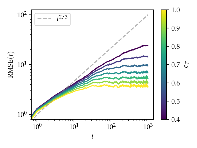
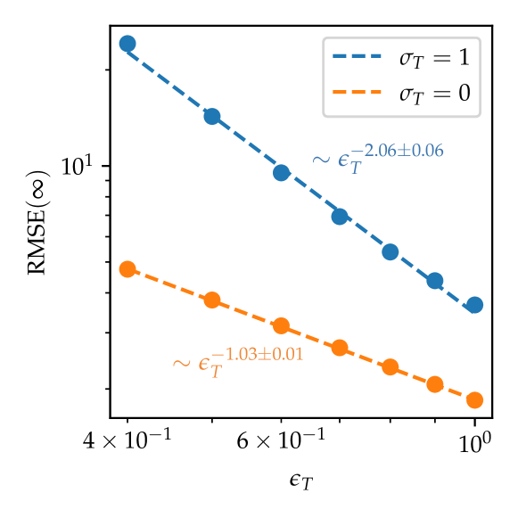
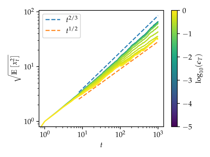
Refer to caption
Figure 3: Plot of root-mean-squared error between true and inferred paths over time $t$ for $\epsilon_{\mathrm{S}}=\sigma_{\mathrm{T}}=\sigma_{\mathrm{S}}=1$. As teacher signal strength $\epsilon_{\mathrm{T}}$ increases, the root-mean-squared error plateaus at smaller values.
Refer to caption
Figure 4: Scaling of estimated long time $\text{RMSE}(\infty)$ with teacher signal strength $\epsilon_{\mathrm{T}}$ for teacher noise strength $\sigma_{\mathrm{T}}=0$ and $\sigma_{\mathrm{T}}=1$. Both cases support power law with $\epsilon_{\mathrm{T}}$, indicating a finite RMSE with any signal. $\sigma_{\mathrm{T}}=0$ case confirms theoretical predictions.

We solve Eq. 10 numerically using $\bm{\phi}_{t}$ generated using $p_{\mathrm{T}}(\bm{\phi}_{t}|x^{*}_{t})$ with $x^{*}_{t}$ sampled from a symmmetric random walk. We set $\epsilon_{\mathrm{S}}=\sigma_{\mathrm{T}}=\sigma_{\mathrm{S}}=1$ unless otherwise specified. Figure 3 shows the RMSE Eq. 15 between the true and inferred positions, $\text{RMSE}(t)$ with maximum time $t_{\max}=1000$, system size $L=1000$ with periodic boundary conditions, as $\epsilon_{\mathrm{T}}$ is varied. We see that for $\epsilon_{\mathrm{T}}$ close to $1$, $\text{RMSE}(t)$ appears to plateau within $t^{*}$ at some $\text{RMSE}(\infty)$. In Fig. 4, for the values of $\epsilon_{\mathrm{T}}$ where we can see a clear plateau, we study the scaling of estimated long-time $\text{RMSE}(\infty)$ with $\epsilon_{\mathrm{T}}$. For $\sigma_{\mathrm{T}}=1$ We see good evidence supporting that $\text{RMSE}(\infty)\sim\epsilon_{\mathrm{T}}^{-2.06(1)}$, which, if the scaling holds for all values of $\epsilon_{\mathrm{T}}>0$, suggests that $\text{RMSE}(t)$ is bounded for any $\epsilon_{\mathrm{T}}>0$. This suggests that $\alpha=1/2$ for any finite $\epsilon_{\mathrm{T}}>0$. For the $\sigma_{\mathrm{T}}=0$ case, the numerics support the $\text{RMSE}(\infty)\sim\epsilon_{\mathrm{T}}^{-1}$ scaling of Eq. (34). This suggests that there is a change in the scaling of $\text{RMSE}(\infty)$ with and without the presence of disorder. We summarise our discussion on the wandering exponents in a conjectured phase diagram in Fig. 5.

$\epsilon_{\mathrm{S}}$ $\alpha=\frac{2}{3}$ $\epsilon_{\mathrm{T}}$ $\alpha=\frac{1}{2}$ $\alpha=\frac{1}{2}$?00$\epsilon_{\mathrm{S}}=\epsilon_{\mathrm{T}}$ $\alpha=\frac{1}{2}$
Figure 5: Conjectured phase diagram for wandering exponents $\alpha$ in the $\epsilon_{\mathrm{S}}-\epsilon_{\mathrm{T}}$ plane with fixed $\sigma_{\mathrm{S}}=\sigma_{\mathrm{T}}=\sigma$. The blue and red texts are analytical results. Numerics appears to support that $\alpha=1/2$ for any finite $\epsilon_{\mathrm{T}}>0$.

In the directed polymer problem $\epsilon_{\mathrm{T}}=0$, there is no transition at finite noise strength $\sigma_{\mathrm{T}}$, and the wandering exponent is $\alpha=2/3$ for any $\sigma_{\mathrm{T}}>0$. Our numerics seems to suggest that the wandering exponent switches immediately to $\alpha=1/2$ for any finite $\epsilon_{\mathrm{T}}>0$. In the language of directed polymers, $\epsilon_{\mathrm{T}}>0$ corresponds to the strength of an attractive delta potential. Our numerics suggest a hierarchy of terms in the polymer’s ‘energy’ Eq. 28: The disordered media term always overcomes the polymer ‘elasticity’ term, while the delta-potential term always beats the disordered media term. In the language of Bayesian inference, inference is always possible with any true signal strength.

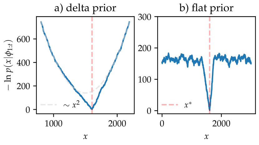
In Fig. 6, we plot a typical free energy profile for a given random walk $x^{*}$ starting from both flat and delta initial priors $p_{\mathrm{S}}(x_{1})\sim 1$ and $\delta_{x_{t},0}$ respectively. We see that amongst the rough landscape corresponding to KPZ (Kardar-Parisi-Zhang) behaviour, we see a ‘linear dispersion’ in the free energy. In the noiseless case, $\sigma_{\mathrm{T}}=0$, Eq. (31) is the imaginary-time Schrödinger equation for a time-varying Hamiltonian with a delta potential located at $x^{*}$, $\hat{H}(t)=-\nu_{\mathrm{S}}\partial^{2}_{x}-\frac{\epsilon_{\mathrm{S}}\epsilon_{\mathrm{T}}}{\sigma_{\mathrm{S}}^{2}}\delta(x-x^{*}(t))$. The instantaneous ground state of $\hat{H}(t)$ is the single bound state given by $q_{0}(x)\sim e^{-\kappa\lvert x-x^{*}\rvert}$, with $\kappa=\frac{\epsilon_{\mathrm{S}}\epsilon_{\mathrm{T}}}{2\nu_{\mathrm{S}}\sigma_{\mathrm{S}}^{2}}$. The imaginary time evolution projects out the ground state, and if the potential moves slowly in time, we expect the $q_{S}(x,t)$ to follow the potential, so that $q_{S}(x,t)\sim e^{-\kappa\lvert x-x^{*}(t)\rvert}$. Taking the logarithm, the free energy should have the form $F\sim-\kappa\lvert x-x^{*}\rvert$. The numerics seems to suggest that this picture from the $\epsilon_{\mathrm{T}}=0$ case persists even in the presence of the random potential.

Refer to caption
Figure 6: An example of the free energy profile $F=-\ln p_{\mathrm{S}}(x_{t}|\phi_{1:t})$ at $t=1000$ for a) delta peak prior b) flat prior. Vertical dashed pink line indicates true position $x^{*}$ and dashed grey line indicates Gaussian modulation due to the delta peak prior.

III.2 Directed polymer mapping

Here, to help with theoretical analysis, we take the continuum limit. Let us work with the separated noise and signal picture as Eq. (24). We define $\tilde{x}=ax$, $\tilde{\tau}=a\tau$, with final time $\tilde{t}=at$, then take the $a\rightarrow 0$ limit with $\tilde{t}$ fixed. Let us assume that the transition kernel $q_{\mathrm{S}}(x_{t}|x_{t-1})$ only depends on the distance between the two points, and that it is maximised when the distance is zero. We take the scaling form $\ln q_{\mathrm{S}}(x_{t}|x_{t-1})=f_{\mathrm{S}}(\sqrt{a}[x_{t}-x_{t-1}])$ then expand around 00. We write $\psi_{x,t}=\sigma_{\mathrm{T}}\eta_{x,t}$, where $\eta_{x,t}\sim\mathcal{N}(0,1)$. Hence we can write the unnormalised posterior as

$\displaystyle q_{S}(x_{t}|\bm{\psi}_{1:t},x^{*}_{1:t})=\sum_{x_{t-1}\cdots x_{1}}\exp\left(\sum_{\tau=1}^{t}\left[-\frac{a}{4\nu_{\mathrm{S}}}\left[x_{\tau}-x_{\tau-1}\right]^{2}+\frac{\epsilon_{\mathrm{S}}\sigma_{\mathrm{T}}}{\sigma_{\mathrm{S}}^{2}}\eta_{x_{\tau},\tau}+\frac{\epsilon_{\mathrm{S}}\epsilon_{\mathrm{T}}}{\sigma_{\mathrm{S}}^{2}}\delta_{x_{\tau},x^{*}_{\tau}}\right]+\mathcal{O}(a^{3/2})\right)q_{S}(x_{1}),$ (26)

where $\nu_{\mathrm{S}}=\frac{1}{2\lvert f^{\prime\prime}_{\mathrm{S}}(0)\rvert}$ is the student’s width of the kernel, and $x_{0}=x_{1}$ for notational convenience. In the $a\rightarrow 0$ limit we have $\sum_{\tau}a\rightarrow\int d\tau$, $\frac{1}{a}\delta_{x_{t},x^{*}_{t}}\rightarrow\delta(\tilde{x}(\tilde{\tau})-\tilde{x}^{*}(\tilde{\tau}))$, and $\frac{ax_{\tau}-ax_{\tau-1}}{a}\rightarrow\frac{d\tilde{x}}{d\tilde{t}}$. We define $\tilde{\eta}_{x,t}:=\frac{1}{a}\eta_{x,t}$ to retrieve white noise at continuum, $\mathbb{E}_{\tilde{\eta}}\tilde{\eta}_{x,t}\tilde{\eta}_{x^{\prime},t^{\prime}}=\frac{1}{a}\delta_{x,x^{\prime}}\frac{1}{a}\delta_{t,t^{\prime}}\rightarrow\delta(\tilde{x}-\tilde{x}^{\prime})\delta(\tilde{t}-\tilde{t}^{\prime})$. Taking the limit then relabeling the continuum variables by removing the tildes, we have

$\displaystyle q_{S}(x_{t}|\eta,x^{*})\sim\int_{p_{\mathrm{S}}(x(0))}^{x(t)=x_{t}}D[x]e^{-E[x,\eta,x^{*}]},$ (27)

where now $\eta$ and $x^{*}$ refer to functions or continuous paths, and the ‘energy’ of the polymer is

$\displaystyle E[x,\eta,x^{*}]=\int_{0}^{t}d\tau\left[\frac{1}{4\nu_{\mathrm{S}}}\dot{x}^{2}-\frac{\epsilon_{\mathrm{S}}\sigma_{\mathrm{T}}}{\sigma_{\mathrm{S}}^{2}}\eta(x(\tau),\tau)-\frac{\epsilon_{\mathrm{S}}\epsilon_{\mathrm{T}}}{\sigma_{\mathrm{S}}^{2}}\delta(x(\tau)-x^{*}(\tau))\right].$ (28)

This is the directed polymer with an attractive moving delta potential located at the path of the random walker $x^{*}(t)$. $p_{\mathrm{S}}(x(0))$ indicates the initial prior distribution. For example, for the Kronecker-delta initial state $p_{\mathrm{S}}(x_{1})=\delta_{x_{1},0}$ we can replace $p_{\mathrm{S}}(x(0))\rightarrow x(0)=0$.

Taking the same limit for the partition function, the normalised posterior can then be written as

$\displaystyle p_{S}(x_{t}|\eta,x^{*})=\frac{\displaystyle q_{S}(x_{t}|\eta,x^{*})}{\displaystyle Z_{P}(t)},$ (29)

where $Z_{P}(t)=\int_{p_{\mathrm{S}}(x(0))}D[x]e^{-E[x,\eta,x^{*}]}$. In the continuum limit, we have $p_{\mathrm{T}}(x_{1:t}^{*})\sim e^{-E_{0}[x^{*}]}p_{\mathrm{T}}(x^{*}(0))$ where $E_{0}=\int_{0}^{t}d\tau\frac{1}{4\nu_{\mathrm{T}}}{(\dot{x}^{*})}^{2}$. Marginalising over $\bm{\eta}_{1:t}$ and $x^{*}_{1:t-1}$ then taking the continuum limit all together, the joint distribution for inferred position and true position at time $t$ is given by

$\displaystyle p(x_{t},x^{*}_{t})$ $\displaystyle=\int D\pi[\eta]\int_{p_{\mathrm{T}}(x^{*}(0))}^{x^{*}(t)=x^{*}_{t}}D[x^{*}]e^{-E_{0}[x^{*}]}\frac{q_{S}(x_{t}|\eta,x^{*})}{Z_{P}(t)}.$ (30)

Just as the directed polymer can be mapped to the KPZ equation and a diffusion process with random sources and sinks, from the path integral picture, we can see that the unnormalised posterior, with abuse of notation $q_{S}(x,t)=q_{S}(x_{t}|\eta,x^{*})$, should evolve as a random diffusion process with a delta potential,

$\displaystyle\frac{\partial q_{S}}{\partial t}=\nu_{\mathrm{S}}\partial_{x}^{2}q_{S}+\left(\frac{\epsilon_{\mathrm{S}}\sigma_{\mathrm{T}}}{\sigma_{\mathrm{S}}^{2}}\eta(x,t)+\frac{\epsilon_{\mathrm{S}}\epsilon_{\mathrm{T}}}{\sigma_{\mathrm{S}}^{2}}\delta(x-x^{*}(t))\right)q_{S},$ (31)

and that the ‘free energy’ $F:=\ln q_{S}(x,t)$ evolves as a KPZ equation with a delta potential,

$\displaystyle\frac{\partial F}{\partial t}$ $\displaystyle=\nu_{\mathrm{S}}\partial_{x}^{2}F+\nu_{\mathrm{S}}(\partial_{x}F)^{2}$
$\displaystyle+\frac{\epsilon_{\mathrm{S}}\sigma_{\mathrm{T}}}{\sigma_{\mathrm{S}}^{2}}\eta(x,t)+\frac{\epsilon_{\mathrm{S}}\epsilon_{\mathrm{T}}}{\sigma_{\mathrm{S}}^{2}}\delta(x-x^{*}(t)).$ (32)

In the planted ensemble picture, we can consider the posterior for path $x_{1:t}$ given $\bm{\phi}_{1:t}$. Following the same procedure to go to the continuum, observables $O[x,x^{*}]$ dependent on entire paths can be formally written as

$\displaystyle\mathop{\mathbb{E}}_{x,\eta,x^{*}}O[x,x^{*}]$ $\displaystyle=\int D\pi[\eta]\int_{p_{\mathrm{T}}(x^{*}(0))}D[x^{*}]e^{-E_{0}[x^{*}]}$ (33)
$\displaystyle\times\frac{\int_{p_{\mathrm{S}}(x(0))}D[x]O[x,x^{*}]e^{-E[x,\eta,x^{*}]}}{Z_{P}(t)}.$

The case $\sigma_{\mathrm{T}}=0$ with the delta initial condition is the short-range interaction limit for the ‘memory model’ considered in Ref. [14], but with open boundary condition at the end times. This case corresponds to the somewhat unrealistic scenario where the student does not know that the images given by the teacher have no noise, and assumes that there is some level of noise. Ref. [14] considers the long-time path-averaged mean squared distance between the student and teacher paths, $\overline{\mathrm{RMSE}}(\infty)$. Translating between the two languages, $1/4\nu_{\mathrm{S}}=\beta/2$, $\beta u=\epsilon_{\mathrm{S}}\epsilon_{\mathrm{T}}/\sigma_{\mathrm{S}}^{2}$, and $1/4\nu_{\mathrm{T}}=\gamma/2$, we find

$\displaystyle\overline{\mathrm{RMSE}}(\infty)\sim\frac{\displaystyle\sigma_{\mathrm{S}}^{2}}{\displaystyle\epsilon_{\mathrm{S}}\epsilon_{\mathrm{T}}}(\nu_{\mathrm{S}}+\nu_{\mathrm{T}}).$ (34)

For the delta initial condition, a quantity of interest is the long-time wandering exponent $\alpha$ that describes the long-time growth of fluctuations $\sqrt{\operatorname*{\mathbb{E}}[x^{2}_{t}]}\sim t^{\alpha}$. In the case $\epsilon_{\mathrm{T}}=0$, we have the directed polymer and have $\alpha=2/3$. In case $\epsilon_{\mathrm{S}}=0$, looking at Eq. (31), we have the heat equation for $q_{\mathrm{S}}$ and have $\alpha=1/2$. In the Bayesian optimal case, $\mathrm{S}=\mathrm{T}$, since the joint distribution is symmetric with $x_{1:t}$ and $x^{*}_{1:t}$, and because the teacher $x^{*}_{1:t}$ undergoes a random walk, we must also have $\alpha=1/2$. What happens away from these limits is not immediately obvious.

Let us argue that $\alpha=1/2$ if $\overline{\mathrm{RMSE}}(\infty)$ is finite for a fixed $\epsilon_{\mathrm{T}}$. Since the RMS distance between the true and inferred paths is bounded, $x_{t}\sim x^{*}_{t}+C$ with $\lvert C\rvert\lesssim\overline{\mathrm{RMSE}}(\infty)$. Since $x^{*}_{t}$ can grow arbitrarily with time, at long times the $x^{*}_{t}$ term dominates and fluctuations of $x_{t}$ should grow as $x^{*}_{t}$ does. In Fig. 7 we plot the RMS width of the inferred position, $\sqrt{\operatorname*{\mathbb{E}}[x^{2}_{t}]}$. We see that for large signal strength $\epsilon_{\mathrm{T}}\sim 1$, the RMS width switches from $\sim t^{2/3}$ to $\sim t^{1/2}$ at some time $t^{*}$. Furthermore as $\epsilon_{\mathrm{T}}$ is lowered we see a crossover from $\alpha=1/2$ to $\alpha=2/3$ for a given finite $t$.

Refer to caption
Figure 7: Plot of root-mean-squared width of the inferred path $\sqrt{\operatorname*{\mathbb{E}}[x^{2}_{t}]}$. At high teacher signal strength $\epsilon_{\mathrm{T}}$ we see that RMS width switches from $\sim t^{2/3}$ to $\sim t^{1/2}$ behaviour at plateau time. As $\epsilon_{\mathrm{T}}$ is lowered we see a crossover to $\sim t^{2/3}$ behaviour at finite time.

IV Tree case

Refer to caption
Figure 8: An example of Bayesian inference on a random walker on a tree with branching number $k=3$, $t=4$, teacher and student signal strengths $\epsilon_{\mathrm{T}}=\epsilon_{S}=2$, and $\sigma_{\mathrm{T}}=\sigma_{\mathrm{S}}=1$. The yellow nodes in the main figure are the true positions of the random walker while the colour of each edge corresponds to the posterior for the path ending at the next node. (Inset) The ‘noisy images’ taken at each timestep.

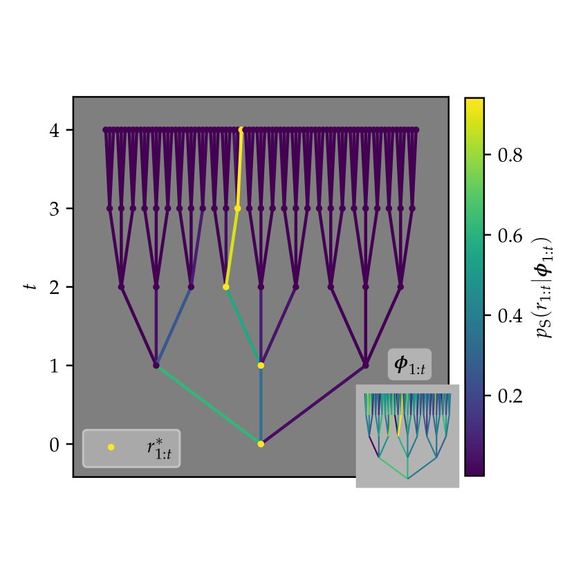
Let us consider the case where the random walker moves in a Cayley tree of depth $t$ with branching number $k$, moving deeper into the tree at each timestep, as shown by the location of the yellow nodes in Fig. 8. On the tree, positions can be labeled by which direction the walker took at each timestep. Therefore we use the string notation $r_{1:t}=r_{1}r_{2}\dots r_{t}$ to denote positions on the tree, where each $r_{\tau}=1,\dots,k$ denotes direction chosen at depth $\tau$. On a tree, there is only one path for a given position. Therefore we also can interpret $r_{1:t}$ as the path taken. If we assume that all branches are equally likely, i.e.

$\displaystyle p(r^{\prime}_{1:t}|r_{1:t-1})=\begin{cases}\frac{1}{k}&\text{if }r^{\prime}_{1:t-1}=r_{1:t-1},\\ 0&\text{otherwise},\end{cases}$ (35)

then the posterior can be written as

$\displaystyle p_{\mathrm{S}}(r_{1:t}|\phi_{1:t})=\frac{e^{\epsilon_{\mathrm{S}}\Phi(r_{1:t})/\sigma_{\mathrm{S}}^{2}}}{Z_{\mathrm{S}}(\Phi)},$ (36)

where we define $\Phi(r_{1:t}):=\phi_{r_{1},1}+\phi_{r_{1:2},2}+\cdots+\phi_{r_{1:t},t}$, and $Z_{\mathrm{S}}(\Phi)=\sum_{r_{1:t}}e^{\epsilon_{\mathrm{S}}\Phi(r_{1:t})/\sigma_{\mathrm{S}}^{2}}$. In Fig. 8, the edges of the main figure are an example of the posterior $p_{\mathrm{S}}(r_{1:t}|\phi_{1:t})$, inferred from the noisy images $\bm{\phi}_{1:t}$ that are represented by the edges of the inset.

For a given inferred path $r_{1:t}$, let $w(r_{1:t},r^{*}_{1:t})$ be the fraction of time which $r_{1:t}$ is equal to the true path, $r^{*}_{1:t}$. Since on the tree, each path is equivalent to every other path, we can fix $r^{*}_{1:t}$ when calculating the overlap. The overlap is then

$\displaystyle\overline{Y}$ $\displaystyle=\mathop{\mathbb{E}}_{r,\Phi}\left[w(r_{1:t},r^{*}_{1:t})\right]$
$\displaystyle=\mathop{\mathbb{E}}_{\Phi}\left[\frac{\sum_{r_{1:t}}w(r_{1:t},r^{*}_{1:t})e^{\epsilon_{\mathrm{S}}\Phi(r_{1:t})/\sigma_{\mathrm{S}}^{2}}}{Z_{\mathrm{S}}(\Phi)}\right].$ (37)

When there is no signal $\epsilon_{\mathrm{T}}=0$, we expect all $k^{t}$ paths to be equally likely. Out of these paths, for a given overlap $wt$, there are $k^{t-1-wt}$ paths. Then the average overlap is a geometric sum,

$\displaystyle\overline{Y}_{\mathrm{unif}}(t)=\frac{1}{t}\sum_{wt=0}^{t}wt\,k^{-1-wt}\xrightarrow{t\gg 1}\frac{1}{t\ln k}.$ (38)

Following the prescription in Eq. (24), we separate the planted potential into iid Gaussian part and the signal part as $\phi_{x,t}=\psi_{x,t}+\epsilon_{\mathrm{T}}\delta_{x,x^{*}_{t}}$. Then, a path $r_{1:t}$ that has overlap $q$ with the true path $r^{*}_{1:t}$ has the energy $\Psi(r_{1:t})+\epsilon_{\mathrm{T}}qt$, where $\Psi_{1:t}(r_{1:t})=\psi_{r_{1},1}+\psi_{r_{1:2},2}+\cdots+\psi_{r_{1:t},t}$ is the unplanted random field. Therefore we can write Eq. (IV) as an expectation on $\Psi$ as

$\displaystyle\overline{Y}=\mathop{\mathbb{E}}_{\Psi}\left[\frac{\sum_{w}wz_{w}(\Psi,r^{*})e^{\epsilon_{\mathrm{S}}\epsilon_{\mathrm{T}}wt/\sigma_{\mathrm{S}}^{2}}}{Z_{P}(\epsilon_{\mathrm{T}},\Psi)}\right],$ (39)

where we introduced the partial partition function

$\displaystyle z_{w}(\Psi,r^{*})=\sum_{\begin{subarray}{c}r_{1:t}\\ w(r_{1:t},r^{*}_{1:t})=w\end{subarray}}e^{\epsilon_{\mathrm{S}}\Psi(r_{1:t})/\sigma_{\mathrm{S}}^{2}},$ (40)

and the total planted partition function now can be written as

$\displaystyle Z_{P}(\epsilon_{\mathrm{T}},\Psi)=\sum_{w}z_{w}(\Psi,r^{*})e^{\epsilon_{\mathrm{S}}\epsilon_{\mathrm{T}}wt/\sigma_{\mathrm{S}}^{2}}.$ (41)

Then $Z_{P}(0,\Psi)$ is the partition function for the directed polymer on a tree.

The directed polymer on a tree has been extensively studied, using the following three methods: the replica method, analogy to traveling waves [12, 15], and as a special case of the so-called generalised random energy model (GREM) [16]. Below, we calculate the overlap between the true and inferred paths using the traveling wave and GREM approaches, and show that they lead to identical results.

IV.0.1 GREM approach

The GREM was developed as an extension to the random energy model (REM), the simplest model for spin glass systems, to include correlations between states.

Starting from the spin glass language, in the GREM, each Ising spin configuration $\sigma=(\sigma_{1},\dots,\sigma_{N})$ is assigned a path $r_{1:t}$ on a tree with total number of paths $k_{1}\cdots k_{t}=2^{N}$, with branching number $k_{i}$ generally varying with depth $i$. Then, each bond on the tree is assigned i.i.d Gaussian random energy with width $\sigma_{i}^{2}$ again varying with depth. Then, each spin configuration is given random but correlated energies corresponding to summing up energies of bonds for that path.

Assigning the ferromagnetic configuration $\sigma=(+1,\dots,+1)$ to the ‘true’ path $r^{*}_{1:t}$, the overlap with the ferromagnetic configuration can loosely be interpreted as the magnetisation (per spin). Then, applying a magnetic field $b$ shifts the energies of the configurations with overlap $w$ by $wbN$.

In the case where with branching numbers and widths are constant with depth, the equations for the overlap with the true path from Bayesian inference and the magnetisation due to a magnetic field coincide and are given by Eq. (39), with inverse temperature $\beta:=\epsilon_{\mathrm{S}}/\sigma_{\mathrm{S}}^{2}$ and magnetic field $b=\epsilon_{\mathrm{T}}t/N$.

The case of the GREM in a magnetic field was studied by Derrida and Gardner in Ref. [16]. There they argue that in the large $N$ limit, the quenched free energy can be approximated via ‘maximum a posteriori’ (MAP) approximation. In our case, where we are interested in the large $t$ limit, this corresponds to

$\displaystyle\lim_{t\rightarrow\infty}f=\max_{w}f_{w},$ (42)

where the quenched free energy (density) is $f:=\frac{1}{t}\mathop{\mathbb{E}}_{\Psi}\left[\ln Z_{P}(\Psi)\right]$ and the partial free energy is

$\displaystyle f_{w}:=\frac{1}{t}\mathop{\mathbb{E}}_{\Psi}\left[\ln z_{w}(\Psi,r^{*}_{1:t})\right]+\beta w\epsilon_{\mathrm{T}}.$ (43)

The GREM undergoes phase transitions, the structure of which is given by determined by the variation in $k_{i}$ and $\sigma^{2}_{i}$. In the constant $k_{i}=k$ and $\sigma^{2}_{i}=\sigma^{2}$ case, the GREM undergoes a single phase transition like the REM.

Due to the structure of the tree, the partial partition function is another GREM 222Note that the partial partition function will have a different branching number in the first timestep, leading to a correction term compared to when there is equal branching numbers. However, this correction is subextensive.. The constant width and branching number case in the large $t$ limit can be solved [12] to be

$\displaystyle\frac{1}{t}\mathop{\mathbb{E}}_{\Psi}\left[\ln z_{w}(\Psi,r^{*}_{1:t})\right]=(1-w)\beta c_{\beta},$ (44)

where the ‘speed of the front’ $c_{\beta}$, whose naming will be made obvious later, is given by

$\displaystyle c_{\beta}=\begin{dcases}c(\beta)&\text{if }\beta\leq\beta_{c},\\ c(\beta_{c})&\text{if }\beta>\beta_{c},\end{dcases}$ (45)

with

$\displaystyle c(\beta)=\frac{1}{\beta}\ln\left(k\int d\psi\rho_{\mathrm{T}}(\psi)e^{-\beta\psi}\right),$ (46)

$\rho_{\mathrm{T}}(\psi)=\pi_{\mathrm{T}}(\psi)$ is the teacher’s distribution of the iid noise, and the critical inverse temperature $\beta_{c}$ is given by $\frac{\partial}{\partial\beta}c(\beta)\rvert_{\beta=\beta_{c}}=0$. The $w$-dependence of Eq. (43) can be found to be

$\displaystyle f_{w}=\begin{dcases}\left(\beta\epsilon_{\mathrm{T}}-\left[\frac{\ln k}{\beta}+\frac{\beta\sigma_{\mathrm{T}}^{2}}{2}\right]\right)w+C_{1}&\text{if }\beta\leq\beta_{c},\\ \left(\beta\epsilon_{\mathrm{T}}-\sigma_{\mathrm{T}}\sqrt{2\ln k}\right)w+C_{2}&\text{if }\beta>\beta_{c},\end{dcases}$ (47)

where $C_{1},C_{2}$ are constants independent of $w$ and $\beta_{c}=\sqrt{2\ln k}/\sigma_{\mathrm{T}}$. As $f_{w}$ is linear in $w$, we see that $w$ that dominates the free energy is either 00 or $1$, determined by the sign of the gradient term. The line where the gradient is zero then gives us the boundary between the two regimes, and can be found to be

$\displaystyle\frac{\epsilon_{\mathrm{T}}}{\sigma_{\mathrm{T}}}=\begin{dcases}\ln k\left(\frac{\epsilon_{\mathrm{S}}\sigma_{\mathrm{T}}}{\sigma_{\mathrm{S}}^{2}}\right)^{-1}+\frac{1}{2}\frac{\epsilon_{\mathrm{S}}\sigma_{\mathrm{T}}}{\sigma_{\mathrm{S}}^{2}}&\text{if }\frac{\epsilon_{\mathrm{S}}\sigma_{\mathrm{T}}}{\sigma_{\mathrm{S}}^{2}}\leq\sqrt{2\ln k},\\ \sqrt{2\ln k}&\text{if }\frac{\epsilon_{\mathrm{S}}\sigma_{\mathrm{T}}}{\sigma_{\mathrm{S}}^{2}}>\sqrt{2\ln k}.\end{dcases}$ (48)

IV.0.2 Traveling waves approach

The overlap can also be calculated using the traveling waves approach. To do this we extend the arguments of [12] to the planted case. Using the structure of the tree, up to a multiplicative constant, the recursion relation for planted partition function can be written as

$\displaystyle Z_{P}(\epsilon_{\mathrm{T}},t+1)=e^{\beta(\psi-\epsilon_{\mathrm{T}})}\left(Z^{(1)}_{P}(\epsilon_{\mathrm{T}},t)+\sum_{i=2}^{k}Z^{(i)}_{P}(0,t)\right),$ (49)

with the initial condition imposed to be $Z_{P}(\epsilon_{\mathrm{T}},0)=1$. We note that $\epsilon_{\mathrm{T}}=0$ retrieves the unplanted partition function of the directed polymer. Defining the planted generating function as

$\displaystyle G_{\epsilon_{\mathrm{T}}}(x,t):=\operatorname*{\mathbb{E}}_{\Psi}\left[\exp(-Z_{P}(\epsilon_{\mathrm{T}},t)e^{-\beta x})\right],$ (50)

the recursion relation of the planted generating function can be written as

$\displaystyle G_{\epsilon_{\mathrm{T}}}(x,t+1)=\operatorname*{\mathbb{E}}_{\psi}\big{[}$ $\displaystyle G_{\epsilon_{\mathrm{T}}}(x+\psi-\epsilon_{\mathrm{T}},t)$ (51)
$\displaystyle\times$ $\displaystyle G_{0}(x+\psi-\epsilon_{\mathrm{T}},t)^{k-1}\big{]},$

where $\psi\sim\mathcal{N}(0,\sigma_{\mathrm{T}}^{2})$ represents noise at a single site/bond.

Let us consider continuous time evolution, where in a timestep $\delta t$, we can have branching with probability $\lambda\delta t$ (so $k=2$), and no branching with probability $(1-\lambda\delta t)$. We renormalise the noise to be $\psi\sim\mathcal{N}(0,2D\delta t)$ and the signal to be $\epsilon_{\mathrm{T}}\cdot 1\rightarrow\epsilon_{\mathrm{T}}\delta t$. Then $G_{\epsilon_{\mathrm{T}}}$ evolves as

$\displaystyle\partial_{t}G_{\epsilon_{\mathrm{T}}}=D\partial_{x}^{2}G_{\epsilon_{\mathrm{T}}}-\epsilon_{\mathrm{T}}\partial_{x}G_{\epsilon_{\mathrm{T}}}-\lambda(1-G_{0})G_{\epsilon_{\mathrm{T}}}.$ (52)

There are three components to Eq. (52). The first term proportional to $D$ is the diffusive term. The second term moves the planted generating function with characteristic velocity $\epsilon_{\mathrm{T}}$ towards the right. The third term is like the non-linear term in the Fisher-Kolmogorov-Petrovsky-Piskunov (FKPP) equation that pushes down $G_{\epsilon_{\mathrm{T}}}(x,t)$ at positions $x$ where $G_{0}(x,t)<1$.

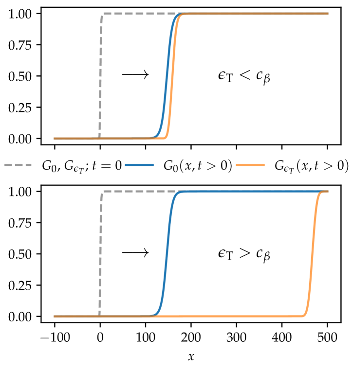
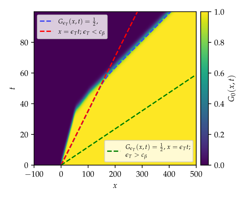
It is known that the unplanted generating function $G_{0}(x,t)$ evolves according to the FKPP equation. In the long time limit, $G_{0}$ moves as a profile that switches from 00 to $1$, and moves with speed $c_{\beta}$ given by Eq. (45), $\lim_{t\rightarrow\infty}G_{0}(x,t)\approx w_{\beta}(x-c_{\beta}t)$, with $w_{\beta}(-\infty)=0$ and $w_{\beta}(\infty)=1$.

$G_{0}$ and $G_{\epsilon_{\mathrm{T}}}$ start with the same initial conditions. If $\epsilon_{\mathrm{T}}<c_{\beta}$, then the third term determines the position of the front and $G_{\epsilon_{\mathrm{T}}}$ moves with the same velocity as $G_{0}$. If $\epsilon_{\mathrm{T}}>c_{\beta}$, then the support of $G_{\epsilon_{\mathrm{T}}}$ moves to a region where $G_{0}=1$ and therefore the third term vanishes, leading to a linear PDE for an error function that moves towards the right with speed $\epsilon_{\mathrm{T}}$ and spreads as $\sqrt{t}$. Therefore $G_{\epsilon_{\mathrm{T}}}$ moves with velocity $v_{\beta,\epsilon_{\mathrm{T}}}=\max(\epsilon_{\mathrm{T}},c_{\beta})$. This is supported and illustrated with numerical simulations in Figs. 9 and 11.

Refer to caption
Figure 9: Numerical simulations of planted and unplanted generating functions. At $t=0$, the unplanted ($G_{0}$) and planted ($G_{\epsilon_{\mathrm{T}}}$) generating functions are equal (grey dashed line). The characteristic velocity of $G_{\epsilon_{\mathrm{T}}}$ is $\epsilon_{\mathrm{T}}$, while $G_{0}$ travels with $c_{\beta}$. (Top) $\epsilon_{\mathrm{T}}=c_{\beta}/2<c_{\beta}$ for $t=60$. $G_{\epsilon_{\mathrm{T}}}$ (orange) sticks to $G_{0}$ (blue). (Bottom) As top but for $\epsilon_{\mathrm{T}}=3c_{\beta}/2>c_{\beta}$. Here we see that $G_{\epsilon_{\mathrm{T}}}$ detaches from $G_{0}$, and moves with its characteristic velocity $\epsilon_{\mathrm{T}}$.

Now $G_{\epsilon_{\mathrm{T}}}(x,t)$ switches from 00 to $1$ approximately at point $\beta\hat{x}\sim\ln Z_{P}(\epsilon_{\mathrm{T}},t)$. From the previous arguments, this point at long times is $\hat{x}(t)=v_{\beta,\epsilon_{\mathrm{T}}}t$. Assuming that fluctuations in $\ln Z_{P}(\epsilon_{\mathrm{T}},t)$ are sublinear, this means that $\operatorname*{\mathbb{E}}_{\Psi}\left[\ln Z_{P}(\epsilon_{\mathrm{T}},t)\right]=\beta v_{\beta,\epsilon_{\mathrm{T}}}t$.

From the definition of average overlap $Y$, we have that $Y=\frac{1}{\beta t}\frac{\partial}{\partial\epsilon_{\mathrm{T}}}\operatorname*{\mathbb{E}}_{\Psi}\left[\ln Z_{P}(\epsilon_{\mathrm{T}},t)\right]=\frac{\partial}{\partial\epsilon_{\mathrm{T}}}v_{\beta,\epsilon_{\mathrm{T}}}$. Then, when $\epsilon_{\mathrm{T}}\leq c_{\beta}$, $v_{\beta,c_{\epsilon_{\mathrm{T}}}}$ does not change with $\epsilon_{\mathrm{T}}$ and therefore $Y=0$. On the other hand, when $\epsilon_{\mathrm{T}}>c_{\beta}$, then we have $\partial_{\epsilon_{\mathrm{T}}}v_{\beta,c_{\epsilon_{\mathrm{T}}}}=1$ and therefore have the overlap of $Y=1$. As $c_{\beta}$ has a phase transition, we must consider the cases when $\beta\leq\beta_{c}$ and $\beta>\beta_{c}$ after which we retrieve the identical phase boundary Eq. (48).

We can generalise to the case where the teacher uses an arbitrary noise distribution, whilst the student conducts inference assuming Gaussian noise. This can be done by choosing a different distribution for $\rho_{\mathrm{T}}(\psi)$ in Eq. 46. The minimum speed is again given by $\partial_{\beta}c(\beta)\rvert_{\beta=\beta_{c}}=0$. For example, for the top-hat distribution $\rho_{T}(\psi)=1/2a$ for $-a<\psi<a$, we have $c(\beta)=\ln\left(k\sinh(\beta a)/\beta a\right)/\beta$, with minimum given at $\beta_{c}=x(k)/a$ for $x\coth(x)-\ln(k\sinh(x)/x)=1$. This is the same qualitative picture as Fig. 10, where $c_{\beta}$ decreases until it hits minimum at some $\beta_{c}$ then freezes. Numerically testing on various unimodal distributions, we consistently found the same qualitative picture.

IV.0.3 Phase diagram and numerics

The phase diagram obtained via either approach with boundary given by Eq. (48) is sketched in Fig. 10.

$\epsilon_{\mathrm{S}}\sigma_{\mathrm{T}}/\sigma_{\mathrm{S}}^{2}$ $\epsilon_{\mathrm{T}}/\sigma_{\mathrm{T}}$ $\sqrt{2\ln k}$ $\sqrt{2\ln k}$00$Y=1$ $Y=0$
Figure 10: Phase diagram for overlap $Y$ on the plane of teacher-student signal strengths $\epsilon_{S}-\epsilon_{T}$ for the case of a tree with branching number $k$. $Y=1$ corresponds to perfect inference whilst $Y=0$ corresponds to failure of inference. The boundary corresponds to a 1st order phase transition.
Refer to caption
Figure 11: (Heatmap) Unplanted generating function ($G_{0}$) evolving according to the FKPP equation. (Blue dashed line) The front of the planted generating function ($G_{\epsilon_{\mathrm{T}}}$), initially moving with characteristic velocity $\epsilon_{\mathrm{T}}=c_{\beta}/2$ (red dashed line) smaller than the unplanted velocity $c_{\beta}$. The front of $G_{\epsilon_{\mathrm{T}}}$ eventually sticks to that of $G_{0}$. (Green dashed line) For characteristic velocities larger than $c_{\beta}$ ($\epsilon_{T}=3c_{\beta}/2>c_{\beta}$), $G_{\epsilon_{\mathrm{T}}}$ is free to travel at $\epsilon_{\mathrm{T}}$.

In the Bayes optimal case, corresponding to the $45^{\circ}$ line on Fig. 10, the planted directed polymer ‘inherits’ the unplanted model’s transition point, $\epsilon/\sigma=\sqrt{2\ln k}$. Additionally, for a given $\epsilon_{\mathrm{T}}/\sigma_{\mathrm{T}}$, one cannot get a greater overlap than the Bayes optimal case.

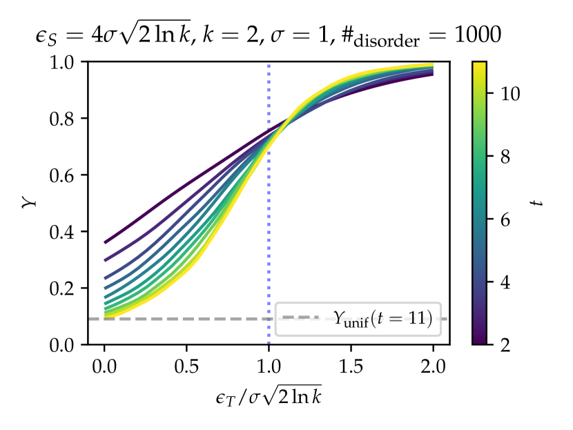
To confirm our theory, in Fig. 12, we numerically study the overlap as we vary time $t$ up to $t=11$ for fixed $\sigma_{\mathrm{S}}=\sigma_{\mathrm{T}}=\sigma=1$, $k=2$, and $\epsilon_{\mathrm{S}}=4\sigma\sqrt{2\ln k}$ for $\#_{\mathrm{disorder}}=1000$ disorder realisations. We confirm the ‘finite size scaling’ of Eq. (38) for $\epsilon_{\mathrm{T}}=0$, and see that the numerics support theoretical transition point $\epsilon^{*}_{T}=\sigma_{\mathrm{T}}\sqrt{2\ln k}$.

Refer to caption
Figure 12: Numerical study of the average overlap $Y$ with teacher signal strength $\epsilon_{T}$ at various times $t$ at fixed branching number $k=2$ and student signal strength $\epsilon_{\mathrm{S}}=4\sigma\sqrt{2\ln k}$. $\#_{\text{disorder}}=1000$ is the number of disorder realisations.

V Conclusion

In this work we introduced the planted directed polymer problem, emphasizing the connections to inference in the planted ensemble, as well as the statistical physics of the directed polymer problem.

Earlier work of Yuille and Coughlan [6] studied tracking of roads in aerial images as a problem of Bayesian inference, including the notion of the planted ensemble. They raised the question of whether there is a fundamental limit to the success of inference in this situation and connected this limit to a phase transition in the thermodynamic limit. They made the further simplification of restricting the paths to a tree, as we did in Section IV, but without connecting to the earlier literature on the directed polymer. They obtain a bound on the ‘error’ $t(1-Y)$ that depends on a regularisation parameter used to treat the $t\rightarrow\infty$ limit but not on $t$. Therefore the regime of vanishing overlap $Y=0$ is not handled correctly. In Ref. [18] the same authors explored the effect of non-optimality due to inference based on the wrong prior.

More recent work of Offer [7] addressed the related problem of Bayesian tracking in clutter using a mean field approximation as well as numerical evaluation of the posterior, finding a phase transition in three or more spatial dimensions. Again, the connection to the directed polymer was not made.

Several avenues for future research exist. One could attempt to adapt existing analytical tools for the $d=1$ directed polymer (such as the replica Bethe ansatz, see e.g. Ref. [19]) to the planted case in order to calculate some of the observables explored in this paper. Moving to higher dimensions, it is known that the directed polymer has a transition at finite disorder strength for $d\geq 3$. We may expect the planted directed polymer to ‘inherit’ the phase transition, as suggested by the investigation of Ref. [7].

Acknowledgements

SWPK and AL acknowledge support from EPSRC DTP International Studentship Grant Ref. No. EP/W524475/1 and EPSRC Critical Mass Grant EP/V062654/1 respectively. We are grateful to Bernard Derrida for useful discussions.

References

  • Zdeborová and Krzakala [2016] L. Zdeborová and F. Krzakala, Advances in Physics 65, 453 (2016).
  • Note [1] Note that throughout we adopt the convention that different distributions are distinguished by the names of their arguments: a convenient abuse of notation.
  • Rabiner and Juang [1986] L. Rabiner and B. Juang, ieee assp magazine 3, 4 (1986).
  • Rabiner [1989] L. R. Rabiner, Proceedings of the IEEE 77, 257 (1989).
  • Welch et al. [1995] G. Welch, G. Bishop, et al.An introduction to the Kalman filter, Tech. Rep. (1995).
  • Yuille and Coughlan [2000] A. L. Yuille and J. M. Coughlan, IEEE Transactions on Pattern Analysis and Machine Intelligence 22, 160 (2000).
  • Offer [2018] C. R. Offer, in 2018 21st International Conference on Information Fusion (FUSION) (IEEE, 2018) pp. 2129–2136.
  • Kardar [2007] M. Kardar, Statistical physics of fields (Cambridge University Press, 2007).
  • Skinner et al. [2019] B. Skinner, J. Ruhman, and A. Nahum, Physical Review X 9, 031009 (2019).
  • Li et al. [2019] Y. Li, X. Chen, and M. P. Fisher, Physical Review B 100, 134306 (2019).
  • Potter and Vasseur [2022] A. C. Potter and R. Vasseur, in Entanglement in Spin Chains: From Theory to Quantum Technology Applications (Springer, 2022) pp. 211–249.
  • Derrida and Spohn [1988] B. Derrida and H. Spohn, Journal of Statistical Physics 51, 817 (1988).
  • Stratonovich [1965] R. L. Stratonovich, in Non-linear transformations of stochastic processes (Elsevier, 1965) pp. 427–453.
  • Dotsenko [2022] V. Dotsenko, Journal of Statistical Mechanics: Theory and Experiment 2022, 093302 (2022).
  • Derrida and Gardner [1986a] B. Derrida and E. Gardner, Journal of Physics C: Solid State Physics 19, 2253 (1986a).
  • Derrida and Gardner [1986b] B. Derrida and E. Gardner, Journal of Physics C: Solid State Physics 19, 5783 (1986b).
  • Note [2] Note that the partial partition function will have a different branching number in the first timestep, leading to a correction term compared to when there is equal branching numbers. However, this correction is subextensive.
  • Yuille and Coughlan [1999] A. L. Yuille and J. Coughlan, in Proceedings. 1999 IEEE Computer Society Conference on Computer Vision and Pattern Recognition (Cat. No PR00149), Vol. 2 (IEEE, 1999) pp. 631–637.
  • Le Doussal and Calabrese [2012] P. Le Doussal and P. Calabrese, Journal of Statistical Mechanics: Theory and Experiment 2012, P06001 (2012).