Exact deconfined gauge structures in the higher-spin Yao-Lee model:
a quantum spin-orbital liquid with spin fractionalization and non-Abelian anyons

Abstract

The spin-S Kitaev model has recently been shown to definitely exhibit topological order with spin liquid ground states for half-integer spin, but could be trivially gapped insulators for integer spin. This interesting “even-odd” effect is largely due to the fermionic (bosonic) $\mathbb{Z}_{2}$ gauge charges for half-integer (integer) spin. In this Letter, we theoretically show that a spin-S Yao-Lee model (a spin-orbital model with SU(2) spin-rotation symmetry) possesses exact deconfined fermionic $\mathbb{Z}_{2}$ gauge charges for any spin (both integer and half integer spin), which implies a topologically-nontrivial quantum spin-orbital liquid (QSOL) ground state regardless of the value of the spin quantum number. We further study the easy-axis limit of the spin-1 Yao-Lee model which can be solved in a controlled perturbative way and show that it exhibits a gapless QSOL ground state, which can even host a non-Abelian topological order by further considering time-reversal breaking interactions to gap out the Dirac cones of the gapless QSOL.

Introduction.—Quantum spin liquids (QSL) [1, 2, 3, 4, 5, 6, 7, 8, 9, 10] are long-range entangled quantum phases beyond the Landau paradigm [11, 12, 13]. Their novel features, such as fractionalized excitations, topological order, and emergent gauge fields, make QSL not only intriguing [14, 15], but also promising candidates for quantum computation [16, 17]. QSL has attracted a great amount of theoretical and numerical studies on frustrated spin models (see, e.g. Refs. [18, 19, 20, 21, 22, 23, 24, 25, 26, 27, 28, 29, 30, 31, 32, 33, 34, 35, 36, 37, 38]); nevertheless some results have been controversial. It is remarkable that various exactly solvable models with QSL ground state have been proposed [39, 40, 41, 42, 43, 44, 45], which were shown exactly to exhibit features of topological order and spin fractionalization. In particular, the seminal spin-$\frac{1}{2}$ exactly solvable Kitaev honeycomb model, originally viewed as a toy model of only theoretical interest, has been shown with increasing experimental evidences that its spin liquid phase can be possibly realized in materials [46, 47, 48, 49].

Besides spin degrees of freedom, localized electrons in many Mott insulators also have orbital degrees of freedom (DOF). A natural route to realize topologically ordered ground states is to further consider orbital DOF of electrons, since orbital DOF may potentially enhance quantum fluctuations [50] and induce fractionalization in spin and/or orbital sectors. Topological liquid states with both spin and orbit DOF are often called QSOL. Possible experimental platforms to realize QSOL include Moiré systems [51, 52, 53]. Numerical evidences of QSOL have been reported in studies on various SU(4) Heisenberg models and Kugel-Khomskii models [53, 54, 55, 56, 57, 51, 52, 58, 59]. Moreover, generalizations of the Kitaev spin-1/2 model to Kugel-Khomskii type spin-orbital interactions have lead to various exactly solvable models with QSOL ground states [60, 61, 62, 63, 64, 65, 66, 67]. In particular, the spin-$\frac{1}{2}$ Yao-Lee model [60] is an exactly solvable spin-orbital model with SU(2) spin-rotation symmetry, which can exhibit non-Abelian spinon excitations. Recently, there have been increasing research interest on the Yao-Lee model and its various extensions [68, 69, 70, 71, 72, 73, 74, 68, 75, 76, 77, 78, 79, 80, 81, 82, 83], which have revealed unexpected fertile physics, such as fermionic magnon [60, 72, 77, 76], fractionalized fermionic criticality [71, 78], order fractionalization [73], and pair-density-wave [69].

More recently higher-spin Kitaev models have attracted numerous research interest [84, 85, 86, 87, 88, 89, 90, 91, 92, 93, 94, 95, 67, 96, 97, 98], partly motivated by their possible experimental realizations [99, 100, 101, 102, 103, 104]. Although the higher-spin Kitaev models are not exactly solvable so far, a novel “even-odd” result somewhat reminiscent of the Haldane conjecture [105] has been established unperturbatively: the ground state must be topologically-nontrivial spin liquids for all half-integer spin, but possibly trivial gapped insulators for integer spin. This even-odd effect is rooted in different natures of the exact $\mathbb{Z}_{2}$ gauge charges in the spin-S Kitaev model, which are fermions and bosons for half-integer and integer spin, respectively. It is then natural to ask whether there exist microscopic models with QSL ground state for all value of spin-S? The integer-spin cases of exactly-solvable QSL models are especially intriguing, since so far no QSL has been obtained in analytically controlled ways for integer-spin Kitaev models (numerical results about their nature are still controversial).

In this work, we show that for the spin-S Yao-Lee model the ground state is always nontrivial QSOL for any value of spin-S. First, we construct the exact $\mathbb{Z}_{2}$ gauge structure in the spin-S Yao-Lee model and show that the deconfined gauge charges are always fermions, which establishes that its ground state must be a QSOL for all spin-S. Secondly, we focus on the spin-1 Yao-Lee model and solve its easy-axis limit perturbatively. The ground state can be gapless QSOL or even has non-abelian topological order. We further show that the zero mode in a $\mathbb{Z}_{2}$ vortex has fractionalized spin quantum number $S^{z}=\frac{1}{2}$, which implies spin fractionalization in the ground state. The physics in the spin-S Yao-Lee model can be richer than the controlled analytical results of spin-S Kitaev models, which either report Abelian $\mathbb{Z}_{2}$ topological order or trivially gapped ground states.

The model.—In this Letter, we mainly focus on the following spin-S Yao-Lee model on the honeycomb lattice:

$$\hat{H}=-\sum_{\langle ij\rangle\in\mu}J_{\mu}[\vec{S}_{i}\cdot\vec{S}_{j}]\otimes[\tau_{i}^{\mu}\tau_{j}^{\mu}],$$ (1)

where $\vec{S}_{i}$ are spin-S operators on site $i$, and the Pauli matrices $\tau_{i}^{\mu}$ represent the orbital degrees of freedom (the case of two orbitals). The spin-spin interactions are nearest-neighbour Heisenberg interactions with SU(2) spin-rotational symmetry, and the orbital interactions are Ising-like, similar to those in the Kitaev honeycomb model, which features Ising couplings $\tau_{i}^{\mu}\tau_{j}^{\mu}$ with coupling constants $J_{\mu}$ in the $\mu=x,y,z$ types of bonds $\langle ij\rangle$, as shown in Fig. 1.

For the case of spin-1/2, namely the spin operators ${\vec{S}}_{i}=\frac{1}{2}{\vec{\sigma}}_{i}$, the Yao-Lee model in Eq. (1) is exactly solvable using Majorana partons [60]. Here we give a brief review of the solution and physical properties of this minimal spin-1/2 Yao-Lee model:

$$\hat{H}_{S=\frac{1}{2}}=-\sum_{\langle ij\rangle\in\mu}\frac{J_{\mu}}{4}\left[\vec{\sigma}_{i}\cdot\vec{\sigma}_{j}\right]\otimes\left[\tau_{i}^{\mu}\tau_{j}^{\mu}\right].$$ (2)

The Pauli operators $\vec{\sigma}_{i}=2\vec{S}_{i}$ and $\vec{\tau}_{i}$ can be written in terms of Majorana fermions: $\vec{\sigma}_{i}=i\vec{d}_{i}d^{0}_{i}$ and $\vec{\tau}_{i}=i\vec{c}_{i}c^{0}_{i}$, where $d_{i}^{0},\vec{d}_{i},c_{i}^{0},\vec{c}_{i}$ are Majorana fermions. The Hilbert space is enlarged with the introduction of these Majorana partons, and one has to impose two constraints on each site to obtain the physical Hilbert space: $d_{i}^{x}d_{i}^{y}d_{i}^{z}d_{i}^{0}=1$ and $c_{i}^{x}c_{i}^{y}c_{i}^{z}c_{i}^{0}=1$. Further, we note that the Majorana bilinears $id_{i}^{0}c_{i}^{0}$ on each site commute with the Hamiltonian, so we can simplify the parton construction by eliminating two Majorana fermions $d_{i}^{0},c_{i}^{0}$ using the projection conditions to get: $\vec{\tau}_{i}=-\frac{i}{2}\vec{c}_{i}\times\vec{c}_{i}$ and $\vec{\sigma}_{i}=-\frac{i}{2}\vec{d}_{i}\times\vec{d}_{i}$. Then, we are left with only one projection each site: $id^{x}_{i}d^{y}_{i}d^{z}_{i}c^{x}_{i}c^{y}_{i}c^{z}_{i}=1$ [60].

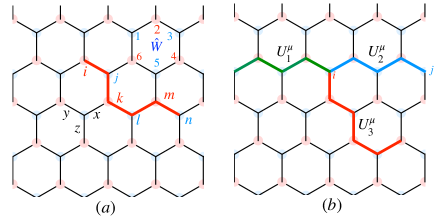
Figure 1: (a) Operator $\hat{W}$ is the flux operator. The red line represents the open string operator. (b) The support of three movement operators $U^{\mu}_{1},U^{\mu}_{2},U^{\mu}_{3}$ of the spin-S spin-orbital model (1) on the lattice. At the ends of each open string operator $U^{\mu}$, there are two excitations which have fermionic statistics and can be moved by $U^{\mu}$.

With the Majorana formulation, the spin-$\frac{1}{2}$ Yao-Lee spin-orbital model in Eq. (2) becomes a quadratic Hamiltonian: $\hat{H}_{S=\frac{1}{2}}^{f}=-\sum_{\langle ij\rangle\in\mu}\frac{J_{\mu}}{4}u_{\langle ij\rangle}[i\vec{d}_{i}\cdot\vec{d}_{j}]$, where the static $\mathbb{Z}_{2}$ gauge field $u_{\langle ij\rangle}=-ic_{i}^{\mu}c_{j}^{\mu}$ satisfies the zero flux condition in the ground state sector. The phase diagram of this spin-1/2 Yao-Lee model is similar to that of the spin-1/2 Kitaev honeycomb model. The ground state has gapped $Z_{2}$ topological order in the anisotropic regime, and it is gapless QSOL with three Dirac cones in the isotropic regime. We may further note that the itinerant fermions in $\hat{H}^{f}_{S=\frac{1}{2}}$ only come from the partons of spin, so the gapless QSOL has no spin order and the spin-spin correlation decays in power-law.

The long-range entangled QSOL in the ground state can be diagnosed even without solving the Hamiltonian. We consider open string operators, as shown in Fig. 1:

$$U^{\mu} =\sigma_{i}^{\mu}\tau_{i}^{y}\tau_{j}^{x}\tau_{k}^{x}\tau_{l}^{z}\tau_{m}^{z}\tau_{n}^{y}\sigma_{n}^{\mu}$$ (3)

$$=id_{i}^{\mu}\left[\hat{u}_{\langle ij\rangle}\hat{u}_{\langle jk\rangle}\hat{u}_{\langle kl\rangle}\hat{u}_{\langle lm\rangle}\hat{u}_{\langle mn\rangle}\right]d_{n}^{\mu}.$$

The end points of $U^{\mu}$ are deconfined fermionic $\mathbb{Z}_{2}$ gauge charges $d_{i}^{\mu}$; since $U^{\mu}$ commutes with the Hamiltonian Eq. (2) except the two end points, the energy cost of separating two gauge charges approaches to a finite constant as their distance goes to infinity. The existence of deconfined fermionic gauge charges in a purely bosonic lattice model can only come from the fractionalization of QSOL. Consequently, we can demonstrate the existence of a QSOL by only referring to the exact $\mathbb{Z}_{2}$ gauge structure without solving the Hamiltonian. In the following, we shall show that deconfined fermionic $\mathbb{Z}_{2}$ gauge charges exist in the spin-S Yao-Lee model in Eq. (1) for any spin-S. This in turn means the ground state of model (1) is always a nontrivial QSOL regardless of the spin-S, including integer spins.

Deconfined fermions in the higher spin Yao-Lee model.—We now construct the exact $\mathbb{Z}_{2}$ gauge structures of the spin-S Yao-Lee model in Eq. (1) through a parton construction, and show that the gauge charges are deconfined fermions for all spin-S. The parton construction here is different from those in the spin-$\frac{1}{2}$ Yao-Lee model and the spin-S Kitaev model [97].

We first decompose the spin-S operator $\vec{S}_{i}$ into 2S spin-$\frac{1}{2}$ Pauli matrices: $\vec{S}_{i}=\frac{1}{2}\sum_{a=1}^{2S}\vec{\sigma}_{a,i}$, together with the projection to leave only the spin-S physical Hilbert space: $(\frac{1}{2}\sum_{a=1}^{2S}\vec{\sigma}_{a,i})^{2}=S(S+1)$. All the Pauli matrices $\vec{\tau}_{i}$ and $\vec{\sigma}_{a,i}$ can now be written into Majorana partons:

$$\vec{\tau}_{i}=-\frac{i}{2}\vec{c}_{i}\times\vec{c}_{i},\quad\vec{\sigma}_{1,i}=-\frac{i}{2}\vec{d}_{1,i}\times\vec{d}_{1,i},$$ (4)

$$\vec{\sigma}_{a,i}=i\vec{d}_{a,i}d_{a,i}^{0},\quad a=2,3,\cdots,2S,$$

where we have eliminated the $c_{i}^{0}$ and $d_{1,i}^{0}$ Majorana fermions in the parton construction of $\vec{\tau}_{i}$ and $\vec{\sigma}_{1,i}$, similar to the spin-$\frac{1}{2}$ model (2). We adopt this construction since the $\mathbb{Z}_{2}$ gauge charges only consist the $d_{i}$ Majorana fermions coming from the fractionalization of spin operators $\vec{S}_{i}$, as we will immediately show below. This implies the spin degrees of freedom can also fractionlize in the QSOL, which is qualitatively different from the pure orbital Kitaev model and has richer physics.

Using this Majorana representation above, the spin-S Yao-Lee spin-orbital model $\hat{{H}}$ can be written as:

$$\hat{H}^{f}=-\frac{1}{4}\sum_{\langle ij\rangle\in\mu}J_{\mu}\hat{u}_{\langle ij\rangle}\sum_{a,b=2}^{2S}i{\vec{D}}_{a,i}\cdot{\vec{D}}_{b,j},$$ (5)

where $\vec{D}_{a,i}=\vec{d}_{1,i}+\vec{d}_{a,i}d_{1,i}^{x}d_{1,i}^{y}d_{1,i}^{z}d_{a,i}^{0}$ is the composite field with $a=2,\cdots,2S$. The $\mathbb{Z}_{2}$ gauge field $\hat{u}_{\langle ij\rangle}=-ic^{\mu}_{i}c_{j}^{\mu}$ are conserved quantities: $\left[\hat{u}_{\langle ij\rangle},\hat{H}^{f}\right]=0$ and $\left[\hat{u}_{\langle ij\rangle},\hat{u}_{\langle i^{\prime}j^{\prime}\rangle}\right]=0$. And it can be directly verified that $\hat{H}^{f}$ is invariant under the local $\mathbb{Z}_{2}$ gauge transformation: $d_{\alpha,i}^{\mu}\rightarrow\Lambda_{i}d_{\alpha,i}^{\mu},\alpha=1,2...2S$ and $\hat{u}_{\langle ij\rangle}\rightarrow\Lambda_{i}\hat{u}_{\langle ij\rangle}\Lambda_{j}$, where $\Lambda_{i}=\pm 1$. As a result, $\hat{u}_{\langle ij\rangle}$ are static $\mathbb{Z}_{2}$ gauge fields with conserved flux on each plaquette. The flux operator can be written in physical operators: $W_{p}=\tau_{1}^{y}\tau_{2}^{z}\tau_{3}^{x}\tau_{4}^{y}\tau_{5}^{z}\tau_{6}^{x}$, as is illustrated in Fig. 1(a).

Now we consider open string operator, e.g. on the string shown in Fig. 1(a):

$$U^{\mu} =e^{i\pi S_{i}^{\mu}}\tau_{i}^{y}\tau_{j}^{x}\tau_{k}^{x}\tau_{l}^{z}\tau_{m}^{z}\tau_{n}^{y}e^{i\pi S_{n}^{\mu}}$$ (6)

$$\propto\Gamma_{i}^{\mu}(\hat{u}^{y}_{\langle ij\rangle}\hat{u}^{z}_{\langle jk\rangle}\hat{u}^{y}_{\langle kl\rangle}\hat{u}^{x}_{\langle lm\rangle}\hat{u}^{y}_{\langle mn\rangle})\Gamma_{n}^{\mu},$$

where the ’$\propto$’ in the second line of the equation above only means there can be a path and spin-S dependent $U(1)$ phase in the parton representation. And $\Gamma_{i}^{\mu}=d_{1,i}^{\mu}\Pi_{a=2}^{2S}(id_{a,i}^{\mu}d_{a,i}^{0})$ are the fermionic $\mathbb{Z}_{2}$ gauge charges at the ends of the open string. The fermionic gauge charges $\Gamma^{\mu}$ are always deconfined regardless of the value of spin-S, since $U^{\mu}$ commutes with $\hat{H}$ except at the two ends of the string such that the energy cost is $O(1)$ when two $\Gamma^{\mu}$ are separated to infinity. As a result, we immediately arrive at the conclusion that the spin-S Yao-Lee model $\hat{H}$ in Eq.(1) always has the nontrivial QSOL ground state for all spin-S !

The fermionic nature of the gauge charges can also be verified in a more fundamental and parton-representation independent way. We can check the statistics of the excitations at the ends of the string using only physical operators, following the approach in [106, 107]. As is illustrated in Fig. 1(b), we suppose there are two excitations located at the sites $i$ and $j$ in the initial state, and we then apply two independent movement sequences $U^{\mu}_{1}U^{\mu}_{2}U^{\mu}_{3}$ and $U^{\mu}_{3}U^{\mu}_{2}U^{\mu}_{1}$ to it, respectively. The two final states only differ by an exchange of the two excitations, so their wave functions will only differ by a statistical phase $\phi$ of the excitations. This is reflected in the algebraic relation of the two movement sequence operators: $U^{\mu}_{1}U^{\mu}_{2}U^{\mu}_{3}=e^{i\phi}U^{\mu}_{3}U^{\mu}_{2}U^{\mu}_{1}$. Here $e^{i\phi}=-1$ for all values of spin-S, which means the excitations at the end points of $U^{\mu}$ obey fermionic statistics.

Having identified the nontrivial QSOL ground state of the spin-S model in Eq. (1), we continue to analyze its physical properties by finding certain limits in which the model is perturbatively solvable. In the following, we shall focus on the easy-axis limit of this model for the case of spin-1. This is the simplest case when the model is not exactly solvable, but it is also very intriguing since the spin-1 Kitaev model does not exhibit spin liquid ground state within analytically controlled solvable limit.

Easy-axis spin-1 Yao-Lee model.—We consider the model in Eq. (1) with spin-1 and $J_{\mu}=J$ in the spin easy-axis anisotropy limit :

$$\hat{H}_{S=1}=-J\sum_{\langle ij\rangle\in\mu}[S_{i}^{z}S_{j}^{z}+a(S_{i}^{x}S_{j}^{x}+S_{i}^{y}S_{j}^{y})]\otimes[\tau_{i}^{\mu}\tau_{j}^{\mu}],~{}~{}~{}$$ (7)

where $0\!<\!a\!\ll\!1$ such that the spin coupling in the z-direction is much larger than those in the x- and y- directions. Here we focus on the case with spatial isotropic couplings $J_{\mu}=J$, where it is possible to obtain a QSOL different from the familiar Abelian $\mathbb{Z}_{2}$ topological order, such as gapless QSOL or even non-Abelian topological order if time-reversal symmetry is broken. Meanwhile, the spatial isotropic coupling limit is the only known regime where the spin-1 Kitaev model may have a spin-liquid ground state, but its nature is still under debate [108, 89]. It is then desired to have an analytically controlled study of the spin-1 model in Eq. (7).

We first derive a low-energy effective Hamiltonian of the model $\hat{H}_{S=1}=\hat{H}_{0}+a\hat{V}$ through a degenerate perturbation up to the order $a^{2}$. Here the unperturbed part $\hat{H}_{0}=-J\sum_{\langle ij\rangle\in\mu}S_{i}^{z}S_{j}^{z}\otimes\tau_{i}^{\mu}\tau_{j}^{\mu}$ is exactly solvable, since all $S_{i}^{z}$s are conserved and we denote the Hamiltonian $\hat{H}_{0}$ with a fixed $\{S_{i}^{z}\}$ configuration as $\hat{H}_{0}(\{S_{i}^{z}\})$. After writing the orbital Pauli matrices $\vec{\tau}_{i}$ into Majorana fermions: $\vec{\tau}_{i}=i\vec{c}_{i}c_{i}^{0}$, $\hat{H}_{0}$ becomes a quadratic fermion Hamiltonian: $\hat{H}_{0}^{f}=-J\sum_{\langle ij\rangle\in\mu}u_{\langle ij\rangle}ic_{i}^{0}c_{j}^{0}$, where $u_{\langle ij\rangle}=-ic_{i}^{\mu}c_{i}^{\mu}S_{i}^{z}S_{j}^{z}$ are static $\mathbb{Z}_{2}$ gauge fields. Due to the $\mathbb{Z}_{2}$ gauge symmetry, an immediate conclusion is that the energy of the ground states of all $\hat{H}_{0}(\{S_{i}^{z}\neq 0\})$ are equal, since these states can be connected to each other through $\mathbb{Z}_{2}$ gauge transformations in the Majorana representation. We denote the set of these states as $\mathcal{G}$ and it can be proved that the ground state subspace of $\hat{H}_{0}$ is $\mathcal{G}$. The detailed proof is shown in the Supplementary Material. Physically, this means that all the ground states to the zeroth order have one Dirac cone and the inclusion of any site with $S^{z}_{i}=0$ will effectively generate a lattice vacancy on that site which increases the energy.

In the ground state sector $\mathcal{G}$ of $\hat{H}_{0}$, $S_{i}^{z}$ can only take two values $\pm 1$, which is like an effectively spin-$\frac{1}{2}$ degrees of freedom. We denote this effective spin-$\frac{1}{2}$ as $\hat{P}S^{z}_{i}\hat{P}=\sigma^{z}_{i}$, where $\hat{P}$ is the projection to the low-energy ground state sector $\mathcal{G}$. A nontrivial effective Hamiltonian can lift the degeneracy of $\mathcal{G}$ at the second order of $a$. As the energy gaps of low-lying intermediate states are approximately the same ($\propto|J|$), we can write down the effective Hamiltonian as:

$$\hat{H}_{\text{eff}}=\hat{P}\hat{H}_{0}\hat{P}-J_{\text{eff}}\sum_{\langle ij\rangle}\left(\sigma_{i}^{x}\sigma_{j}^{x}+\sigma_{i}^{y}\sigma_{j}^{y}-\sigma_{i}^{z}\sigma_{j}^{z}\right),$$ (8)

where $J_{\text{eff}}\propto a^{2}|J|$ and we leave the details of the derivation to the Supplementary Material. For this effective spin-$\frac{1}{2}$ spin-orbital model above, we can use the same Majorana representation as the spin-$\frac{1}{2}$ Yao-Lee model in Eq. (2):

$$\hat{H}_{\text{eff}}^{f}=-J\sum_{\langle ij\rangle}\hat{u}_{ij}\left(id_{i}^{z}d_{j}^{z}\right)$$

$$+2J_{\text{eff}}\sum_{\langle ij\rangle}\left[-id_{i}^{z}d_{j}^{z}(f^{\dagger}_{i}f_{j}+H.c.)+2(\hat{n}_{i}-\frac{1}{2})(\hat{n}_{j}-\frac{1}{2})\right],~{}~{}~{}$$ (9)

where $f_{i}=\frac{1}{2}(d^{x}_{i}-id^{y}_{i})$ or $-\frac{i}{2}(d^{x}_{i}-id^{y}_{i})$ if the site $i$ resides on the A or B sublattice, and $\hat{n}_{i}=f^{\dagger}_{i}f_{i}$. $\hat{u}_{\langle ij\rangle}=-ic^{\mu}_{i}c^{\mu}_{j}$ are static $\mathbb{Z}_{2}$ gauge fields. Since the flux gap is proportional to $|J|$, so we can safely take $\hat{u}_{\langle ij\rangle}=1$.

Although $\hat{H}_{\text{eff}}^{f}$ in Eq. (9) is not directly exactly solvable, we can reliably obtain its ground state properties through a mean-field approximation due to the small parameter $a$. The ground state of $\hat{H}_{0}$ has a Dirac cone with a vanishing density of states, and since $J_{\text{eff}}\ll|J|$, we do not expect this weak four-fermion interaction will induce an symmetry-breaking instability and gap out the Dirac cone. So we propose that the ground state wave function of $\hat{H}_{\text{eff}}^{f}$ in Eq. (9) can be approximated as: $|\psi_{G}\rangle=|d\rangle\otimes|f\rangle$, where $|d\rangle$ and $|f\rangle$ are the $d^{z}$-fermion and $f$-fermion part, respectively. $|d\rangle$ is approximately the ground state of the tight-binding model $\hat{H}_{0,d}=-J\sum_{\langle ij\rangle}id^{z}_{i}d^{z}_{j}$, and $|f\rangle$ is the ground state of:

$$\hat{H}_{\text{f}}=2J_{\text{eff}}\sum_{\langle ij\rangle}\Big{[}-\lambda(f^{\dagger}_{i}f_{j}+H.c.)+2(\hat{n}_{i}-\frac{1}{2})(\hat{n}_{j}-\frac{1}{2})\Big{]},~{}~{}~{}$$ (10)

where $\lambda=\langle id_{i}^{z}d_{j}^{z}\rangle_{d}$ is the expectation value of nearest-neighbour Majorana hopping in the state $|d\rangle$. It is interesting that $\hat{H}_{\text{MF}}$ is just the spinless fermion $t$-$V$ model on the honeycomb lattice (with $t=2\lambda J_{\text{eff}}$ and $V=4J_{\text{eff}}$). Numerically-exact quantum Monte Carlo studies of the honeycomb spinless $t$-$V$ model have reported a phase transition from Dirac semimetal to charge-density-wave (CDW) order with a critical $V/t$: $(V/t)_{c}\approx 1.35$ [109, 110, 111]. As the effective ratio $\frac{V}{t}$ in Eq. (10) is $\frac{V}{t}=\frac{2}{\lambda}>2$, which means the $f$-fermion is in the CDW phase, which, after translating back to the physical degrees of freedom equivalently, implies that the spin exhibits a Neel order with opposite spin moments on different sublattices of the honeycomb lattice. As a result, the easy-axis spin-1 Yao-Lee model in Eq.(7) has the gapless QSOL ground state with a Dirac cone accompanying with the Neel order in the z-direction.

Physically, the spin order in the easy-axis limit is due to the fact that the spin quantum fluctuation is largely suppressed for small $a$. One way to enhance the spin fluctuation is to add a tiny ferromagnetic Ising coupling of the same order as $J_{\text{eff}}$ to the model in Eq. (7): $\hat{H}^{\prime}_{S=1}=\hat{H}_{S=1}+\hat{H}_{\text{FM}}$, where $\hat{H}_{\text{FM}}=-J_{z}\sum_{\langle ij\rangle}S_{i}^{z}S_{j}^{z}$ with $J_{z}>0$. Now the density repulsion in the corresponding $\hat{H}_{\text{MF}}$ is suppressed to $V^{\prime}=4J_{\text{eff}}-2J_{z}$, when $\frac{V^{\prime}}{2\lambda J_{\text{eff}}}$ is smaller than the critical ratio $(\frac{V}{t})_{c}\approx 1.35$, the spin order disappears and the ground state will have three Dirac cones. Specifically, when we take $J_{z}=2J_{\text{eff}}$ in $\hat{H}^{\prime}_{S=1}$ , the density repulsion $V^{\prime}$ of the $f$-fermions in the Marjoana representation is zero up to $a^{2}$, so the ground state must lie in the gapless QSOL phase with three Dirac cones. Then, the spin-spin correlation $\langle S^{z}_{i}S^{z}_{j}\rangle\sim|{\bf r}_{i}-{\bf r}_{j}|^{-4}$ now has power law decay as $|{\bf r}_{i}-{\bf r}_{j}|\rightarrow\infty$ [60], which implies spin also fractionalizes in the QSOL ground state. In below, we give a more direct manifestation of spin fractionalization by showing that the $\mathbb{Z}_{2}$ vortex forms a projective representation of $U(1)_{z}$ spin rotation symmetry if these Dirac cones are gapped.

Non-Abelian topological order.—Having identified the gapless QSOL ground state of the easy-axis spin-1 Yao-Lee model, we further show that non-Abelian topological order can also be realized if time-reversal symmetry (TRS) is spontaneously or explicitly broken in this model.

First, the TRS can be spontaneously broken if we consider the model $\hat{H}^{\prime}_{S=1}$ on the decorated honeycomb lattice (also known as the star lattice) [43], with each site in the honeycomb lattice replaced with three sites of a triangle. For simplicity, we set all the inter-sublattice and intra-sublattice couplings to be the same $J=1$. Its low energy state sector and the effective Hamiltonian are similar to those on the honeycomb lattice, but now the leading order $\hat{H}^{0}$ gaps $d^{z}$ fermions with nonzero Chern number $\nu=\pm 1$. As a result, the weak four-fermion interaction in Eq. (9) which couples $d^{z}$ with $f$ fermions must be irrelevant, and $|\psi_{G}\rangle=|d^{z}\rangle\otimes|f\rangle$ is still a good approximation of the ground state before projection. $|f\rangle$ is the ground state of the quadratic mean field Hamiltonian $\sum_{\langle ij\rangle}\langle id_{i}^{z}d_{j}^{z}\rangle_{d}\left(if^{\dagger}_{i}f_{j}+H.c.\right)$ with $f_{i}=\frac{1}{2}(d_{i}^{x}-id_{i}^{y})$ on all sites , which is also gapped with nonzero Chern number, and the ground state now has non-Abelian Ising topological order. More interestingly, the $\mathbb{Z}_{2}$ vortex has a zero mode which hosts a projective representation of $U(1)_{z}$ spin rotation symmetry with quantum number $S_{z}=\frac{1}{2}$. The reason is similar to that in the spin-$\frac{1}{2}$ Yao-Lee model [60]. Since the $f$-fermions have a nonzero Chern number $\nu=\pm 1$, the $S^{z}$ spin Hall conductance is quantized as $\sigma^{s}_{xy}=\nu\frac{\hbar}{2\pi}$. As a result, if we insert a $\mathbb{Z}_{2}$ $\pi$-flux (or $-\pi$-flux equivalently) in a plaquette, an $S^{z}=\pm\pi\times\sigma^{s}_{xy}=\pm\nu\frac{\hbar}{2}$ will accumulate around the $\mathbb{Z}_{2}$ vortex. This implies the existence of a zero mode with a fractionalized quantum number $S^{z}=\frac{1}{2}$, and the sign of the accumulated spin $S^{z}=\pm\frac{\hbar}{2}$ corresponds to whether the zero mode is occupied or not. Remarkably, the existence of fractionalized $S^{z}=\frac{1}{2}$ in this spin-1 model is a direct evidence of spin fractionalization in the ground state.

Secondly, the TRS can also be explicitly broken on the honeycomb lattice by adding a three-site term to $\hat{H}^{\prime}_{S=1}$ with $J_{z}=2J_{\text{eff}}$:

$$H_{h}=h\sum_{\begin{subarray}{c}\langle ij\rangle\in\alpha\\ \langle jk\rangle\in\beta\end{subarray}}\bm{\epsilon}^{\alpha\beta\gamma}\left[\tau_{i}^{\alpha}\tau_{j}^{\gamma}\tau_{k}^{\beta}\right]\otimes(S^{x}_{i}S^{x}_{k}+S^{y}_{i}S^{y}_{k})^{2},$$ (11)

where $h\ll|J|$ and the three neighbouring sites $i,j,k$ are illustrated in Fig.(1) . A nontrivial effective Hamiltonian in the ground state sector already exists in the first order perturbation of $h$:

$$\Delta H_{h,\text{eff}} = \frac{h}{2}\sum_{\begin{subarray}{c}\langle ij\rangle\in\alpha\\ \langle jk\rangle\in\beta\end{subarray}}\epsilon^{\alpha\beta\gamma}\left(\tau_{i}^{\alpha}\tau_{j}^{\gamma}\tau_{k}^{\beta}\right)\left(\sigma_{i}^{x}\sigma_{k}^{x}+\sigma_{i}^{y}\sigma_{k}^{y}-\sigma_{i}^{z}\sigma_{k}^{z}\right)$$ (12)

$$= \frac{h}{2}\sum_{\langle ij\rangle,\langle jk\rangle}\hat{u}_{ij}\hat{u}_{jk}\left[2i(f^{\dagger}_{i}f_{k}-f^{\dagger}_{k}f_{i})-id_{i}^{z}d_{k}^{z}\right],$$

which gaps all the Majorana fermions with nonzero Chern number and preserves the $U(1)_{z}$ spin rotation symmetry at the same time. The ground state has the Ising nonabelian topological order and fractionalized quantum number $S^{z}=\frac{1}{2}$ in the $\mathbb{Z}_{2}$ vortex. What’s more, we anticipate the accumulated fractionalized charge $S^{z}=\pm\frac{1}{2}$ around the $\mathbb{Z}_{2}$ vortex will persist in the gapless phase as we adiabatically turn off the perturbation $h$, which is also an evidence of spin fractionalization in the gapless QSOL phase.

Concluding remarks.—In this work, we have shown that there exists a spin-orbital model with QSOL ground state for all spin-S by constructing the exact $\mathbb{Z}_{2}$ gauge structure in the spin-S Yao-Lee model. Further, in the minimal integer spin $S=1$ case, we analytically show the ground state can be gapless QSOL or has non-Abelian Ising topological order in the easy-axis limit depending on whether TRS is broken or not. Spin fractionalization is reflected from the accumulated $S^{z}=\pm\frac{1}{2}$ around a $\mathbb{Z}_{2}$ vortex. Our analytical results have revealed richer physics than the controlled solvable anisotropic spin-1 Kitaev model. A generalization of our analysis of the spin-1 Yao-Lee model to higher spin-S would be straightforward. In the future, it would be interesting to go beyond the analytically tractable easy-axis limit and numerically investigate the SU(2) symmetric spin-S Yao-Lee model in Eq.(1).

Acknowledgements: HY is grateful to Prof. Dung-Hai Lee for earlier collaborations on the Yao-Lee model. We also sincerely thank Linhao Li, Zijian Wang, Liujun Zou, and especially Zhou-Quan Wan for helpful discussions. This work is supported in part by NSFC under Grant Nos. 12347107 and 12334003 (ZW, JYZ, and HY), by MOSTC under Grant No. 2021YFA1400100 (HY), and by the Xplorer Prize through the New Cornerstone Science Foundation (HY). ZW acknowledges support from the Shuimu Fellow Foundation at Tsinghua University.

I Supplementary Material

I.1 A. Proof of the ground state subspace

In this section, we prove the low energy ground state sector $\mathcal{G}$ of $\hat{H}_{0}$ in the maintext is given by all the ground state of $\hat{H}_{0}$ with nonzero $S^{z}$. We complete the proof through proof by contradiction.

We suppose $|\psi(\{S^{z}\})\rangle$ is a ground state of $\hat{H}_{0}$ with at least one $S_{i}^{z}=0$, and we prove that its energy must be strictly higher than the real ground state. Actually we only need to consider the states with a single zero $S_{i}^{z}$. Indeed, if there exist at least two zero $S^{z}$: $S_{i}^{z}=S_{j}^{z}=0$ and $j\neq i$ in a state $|\psi^{\prime}\rangle$, then we can add a term $\Delta H_{j}=\eta_{j}\sum_{k\in\langle jk\rangle}S_{k}^{z}\otimes\tau_{j}^{\mu}\tau_{k}^{\mu}$ to $\hat{H}_{0}(\{S^{z}\}^{\prime})$, where $\eta_{j}=\pm 1$ is a $\mathbb{Z}_{2}$ variable to make the expectation value $\langle\psi^{\prime}|\Delta H_{j}|\psi^{\prime}\rangle\leq 0$ and $\{S^{z}\}^{\prime}$ is the $S^{z}$ configuration of $|\psi^{\prime}\rangle$ . Now the ground state energy of the Hamiltonian $\hat{H}_{0}(\{S^{z}\}^{\prime})+\Delta H_{j}$ cannot be higher than the energy of $|\psi^{\prime}\rangle$, but the new ground state has one less zero $S^{z}$. We can continue this process until there is only one zero $S_{i}^{z}$ left, and we only need to prove the energy of the final state $|\psi(\{S^{z}\})\rangle$ is strictly higher than the real ground state of $\hat{H}_{0}$. Meanwhile, an immediate corollary is that the ground states of any $\hat{H}_{0}(\{S^{z}\neq 0\})$ must belong to the real ground states sector of $\hat{H}_{0}$, since we can just continue the addition of $\Delta H$ until no zero $S^{z}$ is left.

Now if $\langle\psi(\{S^{z}\})|\sum_{j\in\langle ij\rangle}S_{j}^{z}\otimes\tau_{i}^{\mu}\tau_{j}^{\mu}|\psi(\{S^{z}\})\rangle\neq 0$, then we can find a nonzero $\eta_{i}$ and the ground state of $\hat{H}(\{S^{z}\})+\Delta H_{i}$ has strictly lower energy and then the proof is complete. So the only corner case left is $\langle\psi(\{S^{z}\})|\sum_{j\in\langle ij\rangle}S_{j}^{z}\otimes\tau_{i}^{\mu}\tau_{j}^{\mu}|\psi(\{S^{z}\})\rangle=0$, and we can prove that this contradicts the assumption that $|\psi(\{S^{z}\})\rangle$ is the ground state of $\hat{H}_{0}$. We write $|\psi(\{S^{z}\})\rangle$ in the Majorana representation: $|\psi(\{S^{z}\})\rangle=\Pi_{i}\hat{D}_{i}|\{u_{\langle ij\rangle}\}\rangle\otimes|c^{0}\rangle$, where $\hat{D}_{i}=\frac{1+c_{i}^{x}c_{i}^{y}c_{i}^{z}c_{i}^{0}}{2}$ is the projection on site $i$. If $\langle\psi(\{S^{z}\})|\sum_{j\in\langle ij\rangle}S_{j}^{z}\otimes\tau_{i}^{\mu}\tau_{j}^{\mu}|\psi(\{S^{z}\})\rangle=0$, then $|\psi(\{S^{z}\})\rangle$ is also the ground state of $\hat{H}_{0}^{\prime}=\hat{H}_{0}(\{S^{z}\})+\sum_{j\in\langle ij\rangle}S_{j}^{z}\otimes\tau_{i}^{\mu}\tau_{j}^{\mu}$. The $S^{z}$ configuration of $\hat{H}_{0}^{\prime}$ has no zero since $S_{i}^{z}=1$, so in the Majorana representation of $\hat{H}_{0}^{\prime}$, we can just take the $\mathbb{Z}_{2}$ gauge field configuration to make the remaining itinerant fermion Hamiltonian preserve all the lattice symmetries, which has only one ground state $|c^{0}\rangle$ with one Dirac cone. As a result, $\langle\psi(\{S^{z}\})|\sum_{j\in\langle ij\rangle}S_{j}^{z}\otimes\tau_{i}^{\mu}\tau_{j}^{\mu}|\psi(\{S^{z}\})\rangle$ is just the expectation value of the summation of three nearest neighbour hoppings: $\sum_{j\in\langle ij\rangle}S_{j}^{z}u_{\langle ij\rangle}\langle c^{0}|ic^{0}_{i}c^{0}_{j}|c^{0}\rangle$, which must be nonzero since $\langle c^{0}|ic^{0}_{i}c^{0}_{j}|c^{0}\rangle$ are the same on all bonds, and $S_{j}^{z}u_{\langle ij\rangle}$ are three $\mathbb{Z}_{2}$ variables whose summation cannot be zero.

I.2 B. Derivation of the effective Hamiltonian through degenerate perturbation

In this section, we derive the effective Hamiltonian of Eq. (8) in the main text through a degenerate perturbation to the second order of a. Since we have identified the zeroth order ground state sector $\mathcal{G}$ in the previous section, which are the ground states of the unperturbed Hamiltonian $\hat{H}_{0}=-J\sum_{\langle ij\rangle\in\mu}S_{i}^{z}S_{j}^{z}\otimes\tau_{i}^{\mu}\tau_{j}^{\mu}$ with all the $S^{z}$ nonzero. So the spin degrees of freedom on each site is an effective spin-$\frac{1}{2}$, and we denote this spin-$\frac{1}{2}$ as: $\hat{P}S^{z}_{i}\hat{P}=\sigma^{z}_{i}$, where $\hat{P}$ is the projection to the low-energy ground state sector $\mathcal{G}$. A nontrivial effective Hamiltonian exists at the second order perturbation:

$$\hat{H}_{\text{eff }}=\hat{P}\hat{H}^{0}\hat{P}+\hat{P}V\left(\frac{1}{E_{0}-\hat{H}_{0}}\hat{Q}V\right)\hat{P},$$ (13)

where $E_{0}$ are the ground state energy of $\hat{H}_{0}$; $\hat{Q}=1-\hat{P}$ is the projection to the excited states, and $V=-aJ\sum_{\langle ij\rangle\in\mu}(S_{i}^{x}S_{j}^{x}+S_{i}^{y}S_{j}^{y})\otimes[\tau_{i}^{\mu}\tau_{j}^{\mu}]$ is the perturbation with $0<a\ll 1$. We assume the energy gap between $\mathcal{G}$ and all the low-lying intermediate states are approximately the same $\Delta|J|$, where $\Delta$ is an $O(1)$ dimensionless postive number, then we can write down a simple form of $\hat{H}_{\text{eff }}$:

$$\hat{P}V\left(\frac{1}{E_{0}-\hat{H}_{0}}QV\right)\hat{P} =-\frac{a^{2}|J|}{\Delta}\hat{P}\left[\sum_{\langle ij\rangle}(S_{i}^{x}S_{j}^{x}+S_{i}^{y}S_{j}^{y})^{2}\right]\hat{P}$$ (14)

$$=-\frac{a^{2}|J|}{\Delta}\sum_{\langle ij\rangle}\hat{P}\left[(S_{i}^{x}S_{j}^{x})^{2}+(S_{i}^{y}S_{j}^{y})^{2}+S_{i}^{x}S_{i}^{y}\otimes S_{j}^{x}S_{j}^{y}+S_{i}^{y}S_{i}^{x}\otimes S_{j}^{y}S_{j}^{x}\right]\hat{P}$$

$$=-\frac{a^{2}|J|}{4\Delta}\sum_{\langle ij\rangle}\left[(\sigma_{i}^{x}+1)(\sigma_{j}^{x}+1)+(\sigma_{i}^{x}-1)(\sigma_{j}^{x}-1)+(\sigma_{i}^{y}+i\sigma_{i}^{z})(\sigma_{j}^{y}+i\sigma_{j}^{z})+(\sigma_{i}^{y}-i\sigma_{i}^{z})(\sigma_{j}^{y}-i\sigma_{j}^{z})\right]$$

$$=-\frac{a^{2}|J|}{2\Delta}\sum_{\langle ij\rangle}\sigma_{i}^{x}\sigma_{j}^{x}+\sigma_{i}^{y}\sigma_{j}^{y}-\sigma_{i}^{z}\sigma_{j}^{z}+\text{const.},$$

where is exactly the Eq. (8) in the main text with $J_{\text{eff}}=\frac{a^{2}|J|}{2\Delta}$.

References

- Anderson [1973] P. Anderson, Materials Research Bulletin 8, 153 (1973).
- Lee [2008] P. A. Lee, Science 321, 1306 (2008).
- Balents [2010] L. Balents, Nature 464, 199 (2010).
- Savary and Balents [2016] L. Savary and L. Balents, Reports on Progress in Physics 80, 016502 (2016).
- Zhou et al. [2017] Y. Zhou, K. Kanoda, and T.-K. Ng, Rev. Mod. Phys. 89, 025003 (2017).
- Knolle and Moessner [2019] J. Knolle and R. Moessner, Annual Review of Condensed Matter Physics 10, 451 (2019).
- Broholm et al. [2020] C. Broholm, R. J. Cava, S. A. Kivelson, D. G. Nocera, M. R. Norman, and T. Senthil, Science 367, eaay0668 (2020).
- Wen [2007] X.-G. Wen, Quantum Field Theory of Many-Body Systems: From the Origin of Sound to an Origin of Light and Electrons (Oxford University Press, 2007).
- Fradkin [2013] E. Fradkin, Field Theories of Condensed Matter Physics, 2nd ed. (Cambridge University Press, 2013).
- Sachdev [2023] S. Sachdev, Quantum Phases of Matter (Cambridge University Press, 2023).
- Levin and Wen [2006] M. Levin and X.-G. Wen, Phys. Rev. Lett. 96, 110405 (2006).
- Kitaev and Preskill [2006] A. Kitaev and J. Preskill, Phys. Rev. Lett. 96, 110404 (2006).
- Wen [2017] X.-G. Wen, Rev. Mod. Phys. 89, 041004 (2017).
- Anderson [1987] P. W. Anderson, Science 235, 1196 (1987).
- Kivelson et al. [1987] S. A. Kivelson, D. S. Rokhsar, and J. P. Sethna, Phys. Rev. B 35, 8865 (1987).
- Kitaev [2003] A. Kitaev, Annals of Physics 303, 2 (2003).
- Nayak et al. [2008] C. Nayak, S. H. Simon, A. Stern, M. Freedman, and S. Das Sarma, Rev. Mod. Phys. 80, 1083 (2008).
- Read and Sachdev [1991] N. Read and S. Sachdev, Phys. Rev. Lett. 66, 1773 (1991).
- Wen [1991] X. G. Wen, Phys. Rev. B 44, 2664 (1991).
- Wen [2002] X.-G. Wen, Phys. Rev. B 65, 165113 (2002).
- Hermele et al. [2005] M. Hermele, T. Senthil, and M. P. A. Fisher, Phys. Rev. B 72, 104404 (2005).
- Yan et al. [2011] S. Yan, D. A. Huse, and S. R. White, Science 332, 1173 (2011).
- Liao et al. [2017] H. J. Liao, Z. Y. Xie, J. Chen, Z. Y. Liu, H. D. Xie, R. Z. Huang, B. Normand, and T. Xiang, Phys. Rev. Lett. 118, 137202 (2017).
- Jiang et al. [2012] H.-C. Jiang, H. Yao, and L. Balents, Phys. Rev. B 86, 024424 (2012).
- Wang and Sandvik [2018] L. Wang and A. W. Sandvik, Phys. Rev. Lett. 121, 107202 (2018).
- Sorella et al. [2012] S. Sorella, Y. Otsuka, and S. Yunoki, Scientific Reports 2, 992 (2012).
- Nomura and Imada [2021] Y. Nomura and M. Imada, Phys. Rev. X 11, 031034 (2021).
- Verresen and Vishwanath [2022] R. Verresen and A. Vishwanath, Phys. Rev. X 12, 041029 (2022).
- Gong et al. [2015] S.-S. Gong, W. Zhu, L. Balents, and D. N. Sheng, Phys. Rev. B 91, 075112 (2015).
- Jiang et al. [2019] Y.-F. Jiang, T. P. Devereaux, and H.-C. Jiang, Phys. Rev. B 100, 165123 (2019).
- He et al. [2017] Y.-C. He, M. P. Zaletel, M. Oshikawa, and F. Pollmann, Phys. Rev. X 7, 031020 (2017).
- Szasz et al. [2020] A. Szasz, J. Motruk, M. P. Zaletel, and J. E. Moore, Phys. Rev. X 10, 021042 (2020).
- Wang et al. [2018] Y.-C. Wang, X.-F. Zhang, F. Pollmann, M. Cheng, and Z. Y. Meng, Phys. Rev. Lett. 121, 057202 (2018).
- Liu et al. [2022a] W.-Y. Liu, S.-S. Gong, Y.-B. Li, D. Poilblanc, W.-Q. Chen, and Z.-C. Gu, Science Bulletin 67, 1034 (2022a).
- Liu et al. [2022b] W.-Y. Liu, J. Hasik, S.-S. Gong, D. Poilblanc, W.-Q. Chen, and Z.-C. Gu, Phys. Rev. X 12, 031039 (2022b).
- Song et al. [2019] X.-Y. Song, C. Wang, A. Vishwanath, and Y.-C. He, Nature Communications 10, 4254 (2019).
- Song et al. [2020] X.-Y. Song, Y.-C. He, A. Vishwanath, and C. Wang, Phys. Rev. X 10, 011033 (2020).
- Qian and Qin [2023] X. Qian and M. Qin, arXiv:2309.13630 (2023).
- Rokhsar and Kivelson [1988] D. S. Rokhsar and S. A. Kivelson, Phys. Rev. Lett. 61, 2376 (1988).
- Moessner and Sondhi [2001] R. Moessner and S. L. Sondhi, Phys. Rev. Lett. 86, 1881 (2001).
- Yao and Kivelson [2012] H. Yao and S. A. Kivelson, Phys. Rev. Lett. 108, 247206 (2012).
- Kitaev [2006] A. Kitaev, Annals of Physics 321, 2 (2006).
- Yao and Kivelson [2007] H. Yao and S. A. Kivelson, Phys. Rev. Lett. 99, 247203 (2007).
- Feng et al. [2007] X.-Y. Feng, G.-M. Zhang, and T. Xiang, Phys. Rev. Lett. 98, 087204 (2007).
- Lee et al. [2007] D.-H. Lee, G.-M. Zhang, and T. Xiang, Phys. Rev. Lett. 99, 196805 (2007).
- Jackeli and Khaliullin [2009] G. Jackeli and G. Khaliullin, Phys. Rev. Lett. 102, 017205 (2009).
- Rau et al. [2016] J. G. Rau, E. K.-H. Lee, and H.-Y. Kee, Annual Review of Condensed Matter Physics 7, 195 (2016).
- Hermanns et al. [2018] M. Hermanns, I. Kimchi, and J. Knolle, Annual Review of Condensed Matter Physics 9, 17 (2018).
- Trebst and Hickey [2022] S. Trebst and C. Hickey, Physics Reports 950, 1 (2022).
- Feiner et al. [1997] L. F. Feiner, A. M. Oleś, and J. Zaanen, Phys. Rev. Lett. 78, 2799 (1997).
- Keselman et al. [2020] A. Keselman, B. Bauer, C. Xu, and C.-M. Jian, Phys. Rev. Lett. 125, 117202 (2020).
- Zhang et al. [2021] Y.-H. Zhang, D. N. Sheng, and A. Vishwanath, Phys. Rev. Lett. 127, 247701 (2021).
- Xu and Balents [2018] C. Xu and L. Balents, Phys. Rev. Lett. 121, 087001 (2018).
- Corboz et al. [2012] P. Corboz, M. Lajkó, A. M. Läuchli, K. Penc, and F. Mila, Phys. Rev. X 2, 041013 (2012).
- Natori et al. [2019] W. M. H. Natori, R. Nutakki, R. G. Pereira, and E. C. Andrade, Phys. Rev. B 100, 205131 (2019).
- Jin et al. [2023] H.-K. Jin, W. M. H. Natori, and J. Knolle, Phys. Rev. B 107, L180401 (2023).
- Wang and Vishwanath [2009] F. Wang and A. Vishwanath, Phys. Rev. B 80, 064413 (2009).
- Zhang et al. [2023] C. Zhang, H.-K. Jin, and Y. Zhou, arXiv:2311.02639 (2023).
- Jin et al. [2022a] H.-K. Jin, R.-Y. Sun, H.-H. Tu, and Y. Zhou, Science Bulletin 67, 918 (2022a).
- Yao and Lee [2011] H. Yao and D.-H. Lee, Phys. Rev. Lett. 107, 087205 (2011).
- Yao et al. [2009] H. Yao, S. C. Zhang, and S. A. Kivelson, Phys. Rev. Lett. 102, 217202 (2009).
- Nussinov and Ortiz [2009a] Z. Nussinov and G. Ortiz, Phys. Rev. B 79, 214440 (2009a).
- Wu et al. [2009] C. Wu, D. Arovas, and H.-H. Hung, Phys. Rev. B 79, 134427 (2009).
- Chua et al. [2011] V. Chua, H. Yao, and G. A. Fiete, Phys. Rev. B 83, 180412 (2011).
- de Farias et al. [2020] C. S. de Farias, V. S. de Carvalho, E. Miranda, and R. G. Pereira, Phys. Rev. B 102, 075110 (2020).
- Nussinov and Ortiz [2009b] Z. Nussinov and G. Ortiz, Phys. Rev. B 79, 214440 (2009b).
- Natori et al. [2023] W. M. H. Natori, H.-K. Jin, and J. Knolle, Phys. Rev. B 108, 075111 (2023).
- Chulliparambil et al. [2021] S. Chulliparambil, L. Janssen, M. Vojta, H.-H. Tu, and U. F. P. Seifert, Phys. Rev. B 103, 075144 (2021).
- Coleman et al. [2022] P. Coleman, A. Panigrahi, and A. Tsvelik, Phys. Rev. Lett. 129, 177601 (2022).
- Sanyal et al. [2021] S. Sanyal, K. Damle, J. T. Chalker, and R. Moessner, Phys. Rev. Lett. 127, 127201 (2021).
- Seifert et al. [2020] U. F. P. Seifert, X.-Y. Dong, S. Chulliparambil, M. Vojta, H.-H. Tu, and L. Janssen, Phys. Rev. Lett. 125, 257202 (2020).
- Natori and Knolle [2020] W. M. H. Natori and J. Knolle, Phys. Rev. Lett. 125, 067201 (2020).
- Tsvelik and Coleman [2022] A. M. Tsvelik and P. Coleman, Phys. Rev. B 106, 125144 (2022).
- Chulliparambil et al. [2020] S. Chulliparambil, U. F. P. Seifert, M. Vojta, L. Janssen, and H.-H. Tu, Phys. Rev. B 102, 201111 (2020).
- Akram et al. [2023] M. Akram, E. M. Nica, Y.-M. Lu, and O. Erten, Phys. Rev. B 108, 224427 (2023).
- Zhuang and Marston [2021] Z. Zhuang and J. B. Marston, Phys. Rev. B 104, L060403 (2021).
- de Carvalho et al. [2018] V. S. de Carvalho, H. Freire, E. Miranda, and R. G. Pereira, Phys. Rev. B 98, 155105 (2018).
- Ray et al. [2021] S. Ray, B. Ihrig, D. Kruti, J. A. Gracey, M. M. Scherer, and L. Janssen, Phys. Rev. B 103, 155160 (2021).
- Poliakov et al. [2023] V. Poliakov, W.-H. Kao, and N. B. Perkins, arXiv:2312.17359 (2023).
- Polyakov and Perkins [2023] V. A. Polyakov and N. B. Perkins, Journal of Experimental and Theoretical Physics 137, 533 (2023).
- Lai and Motrunich [2011] H.-H. Lai and O. I. Motrunich, Phys. Rev. B 84, 235148 (2011).
- Seifert and Moroz [2024] U. F. P. Seifert and S. Moroz, arXiv:2306.09405 (2024).
- Mandal [2024] I. Mandal, arXiv:2401.08568 (2024).
- Oitmaa et al. [2018] J. Oitmaa, A. Koga, and R. R. P. Singh, Phys. Rev. B 98, 214404 (2018).
- Baskaran et al. [2008] G. Baskaran, D. Sen, and R. Shankar, Phys. Rev. B 78, 115116 (2008).
- Koga et al. [2018] A. Koga, H. Tomishige, and J. Nasu, Journal of the Physical Society of Japan 87, 063703 (2018).
- Zhu et al. [2020] Z. Zhu, Z.-Y. Weng, and D. N. Sheng, Phys. Rev. Res. 2, 022047 (2020).
- [88] T. Minakawa, J. Nasu, and A. Koga, Magnetic properties of the s = 1 kitaev model with anisotropic interactions, in Proceedings of the International Conference on Strongly Correlated Electron Systems (SCES2019).
- Lee et al. [2020] H.-Y. Lee, N. Kawashima, and Y. B. Kim, Phys. Rev. Res. 2, 033318 (2020).
- Lee et al. [2021] H.-Y. Lee, T. Suzuki, Y. B. Kim, and N. Kawashima, Phys. Rev. B 104, 024417 (2021).
- Khait et al. [2021] I. Khait, P. P. Stavropoulos, H.-Y. Kee, and Y. B. Kim, Phys. Rev. Res. 3, 013160 (2021).
- Chen et al. [2022] Y.-H. Chen, J. Genzor, Y. B. Kim, and Y.-J. Kao, Phys. Rev. B 105, L060403 (2022).
- Bradley and Singh [2022] O. Bradley and R. R. P. Singh, Phys. Rev. B 105, L060405 (2022).
- Gordon and Kee [2022] J. S. Gordon and H.-Y. Kee, Phys. Rev. Res. 4, 013205 (2022).
- Jin et al. [2022b] H.-K. Jin, W. M. H. Natori, F. Pollmann, and J. Knolle, Nature Communications 13, 3813 (2022b).
- Rousochatzakis et al. [2018] I. Rousochatzakis, Y. Sizyuk, and N. B. Perkins, Nature Communications 9, 1575 (2018).
- Ma [2023] H. Ma, Phys. Rev. Lett. 130, 156701 (2023).
- Liu et al. [2023] R. Liu, H. T. Lam, H. Ma, and L. Zou, arXiv:2310.16839 (2023).
- Xu et al. [2018] C. Xu, J. Feng, H. Xiang, and L. Bellaiche, npj Computational Materials 4, 57 (2018).
- Stavropoulos et al. [2019] P. P. Stavropoulos, D. Pereira, and H.-Y. Kee, Phys. Rev. Lett. 123, 037203 (2019).
- Xu et al. [2020] C. Xu, J. Feng, M. Kawamura, Y. Yamaji, Y. Nahas, S. Prokhorenko, Y. Qi, H. Xiang, and L. Bellaiche, Phys. Rev. Lett. 124, 087205 (2020).
- Stavropoulos et al. [2021] P. P. Stavropoulos, X. Liu, and H.-Y. Kee, Phys. Rev. Res. 3, 013216 (2021).
- Samarakoon et al. [2021] A. M. Samarakoon, Q. Chen, H. Zhou, and V. O. Garlea, Phys. Rev. B 104, 184415 (2021).
- Cen and Kee [2023] J. Cen and H.-Y. Kee, Phys. Rev. B 107, 014411 (2023).
- Haldane [1983] F. D. M. Haldane, Phys. Rev. Lett. 50, 1153 (1983).
- Levin and Wen [2003] M. Levin and X.-G. Wen, Phys. Rev. B 67, 245316 (2003).
- Kawagoe and Levin [2020] K. Kawagoe and M. Levin, Phys. Rev. B 101, 115113 (2020).
- Dong and Sheng [2020] X.-Y. Dong and D. N. Sheng, Phys. Rev. B 102, 121102 (2020).
- Wang et al. [2014] L. Wang, P. Corboz, and M. Troyer, New Journal of Physics 16, 103008 (2014).
- Li et al. [2015a] Z.-X. Li, Y.-F. Jiang, and H. Yao, Phys. Rev. B 91, 241117 (2015a).
- Li et al. [2015b] Z.-X. Li, Y.-F. Jiang, and H. Yao, New Journal of Physics 17, 085003 (2015b).
- Note [1] We still assume cancels the antiferromagnetic Ising couplings arising from the second order perturbation to simplify the discussion.