Smearing of primordial gravitational waves
Abstract
A mechanism for smearing of the primordial gravitational waves during the radiation-dominated phase of the evolution of the Universe is considered. It is shown that the primordial gravitational waves can possess hyperbolicity features due to their propagation through the matter inhomogeneities. This mechanism of smearing can lead to the flattening of the original gravitational wave spectrum and hence has to be taken into account at the interpretation of the properties of primordial gravitational background on the detection of which are oriented ongoing and forthcoming experimental facilities.
pacs:
98.80.-kCosmology1 Introduction
Primordial gravitational waves are considered as potentially unique tools for the study of the very early phases of the Universe, including the features of the inflationary models St1 ; St2 . The studies of theoretical models of production of primordial gravitational waves, of their basic properties, as well as the prospects of their experimental detection were essentially broadened upon the ongoing measurements by LIGO-Virgo-Kagra collaboration, NANOGrav consortium Kam ; Koh ; Wang ; Bal ; Chang ; Yu and references therein. New possibilities regarding the study of primordial gravitational waves can be provided by forthcoming LISA interferometer, e.g. Ric . It is outlined that, primordial gravitational wave background, when detected, can open an entirely new window to a broad scope of effects, as did the detection of the electromagnetic primordial waves, the Cosmic Microwave Background (CMB). Indeed, the latter enabled probing not only the effects at the last scattering surface but also before and after, including the features of the large scale matter distribution, cosmic voids, clusters of galaxies via gravitational lensing, etc Mukhanov ; Holz .
It is believed that, first, the primordial gravitational waves have to be originated from quantum fluctuations St1 , second, then had freely propagated during the subsequent expansion of the Universe, largely keeping their original features. Therefore their features, when detected, are expected to provide a direct insight to the inflationary phase, on the involved scalar fields, on the particle production, etc, for details, see Cap .
Below, we consider a tiny effect which nevertheless can influence the study and interpretation of the properties of the primordial gravitational waves, since this effect provides a principal possibility of the smearing of those properties at radiation-dominated phase of the evolution of the Universe. Namely, we study the propagation of gravitational waves in that phase of the Universe and reveal the conditions for their instability (hyperbolicity) due to matter inhomogeneities which can smear their primordial signatures. This mechanism is dealing with the geodesic flows as formulated in the theory of dynamical systems An ; Arn , and, for example, enabled to reveal the hyperbolicity of the photon beams induced at their propagation within cosmic voids GCMB ; GK1 ; GK2 . The hyperbolicity of geodesic flows was instrumental to conclude regarding the void nature of the Cold Spot spot , a non-Gaussian anomaly in the CMB sky, by means of the estimation of Kolmogorov stochasticity parameter and using the Planck satellite’s data. Hyperbolicity of photon beams depending on the parameters of the cosmic voids and their redshifts and its role in the analysis of the high redshift galactic surveys is studied in Sam1 ; Sam2 ; Sam3 .
Another aspect of the importance of the detection and accurate interpretation of the gravitational wave background besides addressing the early cosmos and high energy physics scale is also expected in the probing of modified gravity theories Capo ; GS and other approaches regarding the cosmological (observational) tensions Val ; Hu ; Ri . Note, that, NANOGrav and collaboration data Ar ; Ag on the nano-hertz gravitational wave background are already used to constrain modified gravity theories, (see, e.g. Can and references therein), thus complementing the other means of high accuracy testing of General Relativity ZNP ; Kop ; C1 ; C2 .
2 The perturbed metric
We consider scalarly perturbed Robertson-Walker metric Holz
| (1) |
where depends on all four coordinates . The matrix form of the metric is
| (2) |
The energy-momentum tensor is given by
| (3) |
where is a unit timelike vector , . For the metric (1) it satisfies
| (4) | |||
| (5) |
Then the non-vanishing components of the energy-momentum tensor for scalarly perturbed Robertson-Walker metric are
| (6) | |||
| (7) | |||
| (8) | |||
| (9) |
We also can write down non-vanishing components of Einstein tensor for the metric (1)
| (10) | |||
| (11) | |||
| (12) | |||
| (13) |
where is the spatial derivative operator. Here we have introduced a notation for the spatial metric as in Holz .
3 Geodesics in presence of scalar perturbations
The averaged geodesic deviation (Jacobi) equation has the form (see GK1 ; Sam1 ),
| (18) |
where is the scalar curvature of space (without conformal factor). Consider the metric
| (19) |
For this metric the spatial scalar curvature takes the form
| (20) |
The gravitational potential satisfies the following equations (see section (7.3.1), Eqs. (7.47)-(7.49) of Mukhanov )
| (21) | |||
| (22) | |||
| (23) |
Here are the covariant spatial components (gauge-invariant) of the 4-velocity of the fluid element. Combining (21) and (23), one can write (section (7.3.1), eq. (7.51) of Mukhanov )
| (24) |
The pressure fluctuation is related to the energy density and entropy perturbations
| (25) |
Let us consider adiabatic perturbations for which , at the domination of relativistic matter with equation of state , where is a positive constant. In this case
| (26) |
For plane wave perturbations , eq. (24) becomes
| (27) |
The solution of this equation is given in terms of Bessel functions
| (28) |
where and are constants. In a radiation dominated case, when , the order of Bessel function is , and the solution (28) can be expressed in terms of elementary functions
| (29) |
where . We can solve eq.(18) for the above and find the distortion of the flow, which will determine the geodesics behavior in this perturbed background. For the plane wave the Ricci scalar (20) becomes
| (30) |
and since , the averaged geodesics equation (18) becomes
| (31) |
Note that, for with constant . For (31) becomes
| (32) |
where .
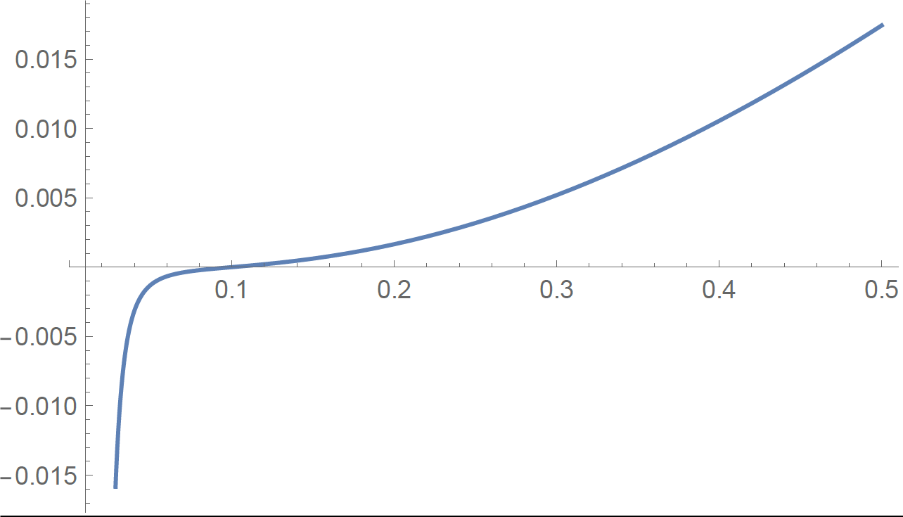
3.1 case
Let us denote . When , then and equation (32) then becomes
| (33) |
The solution to this equation is given by
| (34) |
where and are Bessel functions of the first and second kind, respectively, and and are constants and can be expressed in terms of and for :
| (35) | |||
| (36) |
Plugging and back, we find
| (37) |
The dependance is given in Figure 1. The energy density perturbation in this case, for the solution (29) becomes
| (38) |
Thus, corresponds to the case of high density regions.
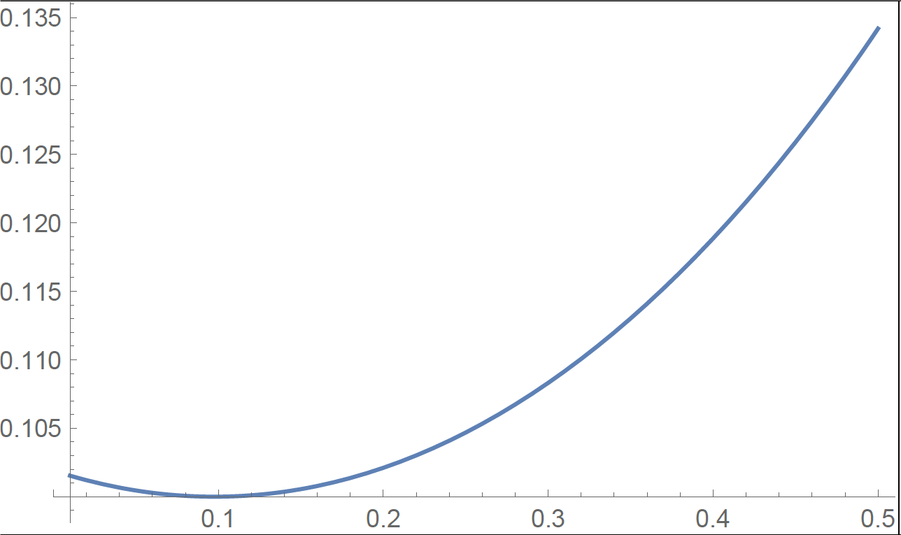
3.2 case
In this case, let us introduce the variable . The minus sign ensures that grows along the time flow. The equation that we have to solve in this case becomes
| (39) |
In this case the solution is given by
| (40) |
Again finding constants and and plugging them back, we find
| (41) |
The dependance is given in Figure 2. From equation (38) it follows that the case corresponds to low density regions.

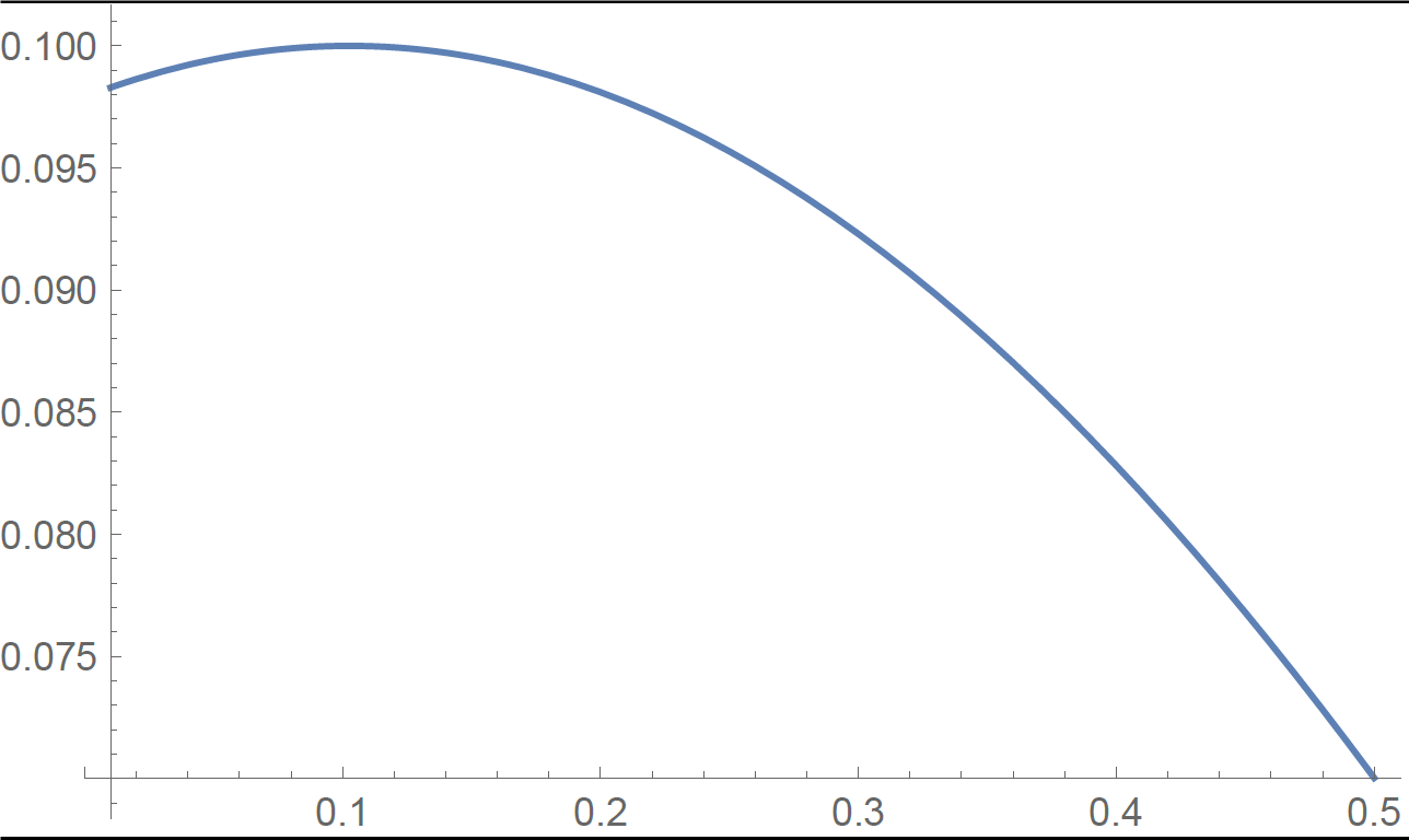
3.3 case
For , and the Jacobi equation (18) takes the form
| (42) |
where . Its solution is given as
| (43) |
where and are constants and can be expressed in terms of , .
| (44) |
Plugging the constants back in (43), we get
| (45) |
The energy density perturbation for is
| (46) |
Hence corresponds to low density, while is for high density regions. Thus, we have
| (47) |
and for the high density regions
| (48) |
Figures 3 and 4 present the corresponding dependencies, in the normalization of the formulae above. The figures clearly reveal the hyperbolicity of the geodesic flow due to the low density regions.
4 Conclusions
We studied the hyperbolicity properties of the primordial gravitational waves due to the inhomogeneities in the radiation-dominated Universe. The behavior of geodesic flows in perturbed metric is studied analysing the solutions of the Jacobi equation of geodesic deviation enabling to trace the hyperbolicity features. The revealed hyperbolicity of the gravitational waves has to smear their original properties.
Then the considered effect of smearing of primordial gravitational wave background is related to the following principal issue. It is expected that the primordial gravitational waves are preserving their properties, thus enabling direct comparison with the theoretical predictions regarding their origin in quantum fluctuations in very early Universe. However, in the case of smearing of the gravitational waves the recovering of the particular details of the inflationary phase, the scalar fields, etc, from the future experimental data would imply far more complicated procedure. If the smearing is occurring at the radiation-dominated phase, then it can be used for distinguishing of any gravitational background signal from a signal originated in matter-dominated phase, as e.g. due to supermassive black hole binaries believed to cause the nano-hertz signal detected by NANOGrav.
The remarkable consequence of the smearing effect can be the flattening of the original spectrum of the gravitational wave background. The spectrum’s flattening effect quantitatively has to be determined by such descriptors, as the Kolmogorov-Sinai (KS)-entropy Kolm defining the mixing properties of geodesic flows and the decay of correlation functions Arn ; Pol ; GK1 . Namely, the correlation function of the geodesic flow defined as
| (49) |
on the unit tangent bundle of Riemannian 3-manifold with negative constant curvature decreases by exponential law for all functions (see Pol for details)
| (50) |
here is the Liouville measure, . KS-entropy in this case has to be determined by the scales of the inhomogeneities in the radiation-dominated Universe GK2 . Thus, the considered effect of smearing can have direct consequences in the interpretation of the observational data on the primordial gravitational wave background, opening also a way to probe the density inhomogeneities in the radiation-dominated phase, linked to the cosmological tensions and modified gravity theories.
5 Acknowledgment
We thank the referee for valuable comments. M.S. is acknowledging the ANSEF grant 23AN:PS-astroth-2922.
6 Data Availability Statement
Data sharing not applicable to this article as no datasets were generated or analysed during the current study.
References
- (1) A. A. Starobinsky, JETP Lett. 30, 682 (1979)
- (2) A. A. Starobinsky, Phys. Lett. B91, 99 (1980)
- (3) M. Kamionkowski and E. D. Kovetz, Ann. Rev. Astron. Astrophys. 54, 227 (2016)
- (4) K. Kohri, T. Terada, Phys. Rev. D97, 123532 (2018)
- (5) S. Wang, T. Terada, and K. Kohri, Phys. Rev. D, 99, 103531 (2019)
- (6) S. Balaji, G. Domenech, and J. Silk, JCAP 09, 016, (2022)
- (7) Z. Chang, X. Zhang, and J.-Z. Zhou, Phys. Rev. D, 107, 063510 (2023)
- (8) Y. Yu, S. Wang, arXiv:2303.03897
- (9) A. Ricciardone, J. Phys.: Conf. Ser. 840, 012030 (2017)
- (10) V. Mukhanov, Physical foundations of cosmology, (Cambridge University Press, 2005)
- (11) D. E. Holz, R. M. Wald, Phys. Rev. D, 58, 063501 (1998)
- (12) C. Caprini, D. G. Figueroa, Class. Quantum Grav. 35, 163001 (2018)
- (13) D.V. Anosov, Geodesic flows on closed Riemannian manifolds of negative curvature, Commun. Steklov Math. Inst., 90, 1 (1967)
- (14) V.I. Arnold, Mathematical Methods of Classical Mechanics (Springer, Berlin, 1989)
- (15) V.G. Gurzadyan, P. De Bernardis, et al, Mod. Phys. Lett. A 20, 813 (2005)
- (16) V.G. Gurzadyan, A. Kocharyan, Eur. Phys. Lett. 86, 29002 (2009)
- (17) V.G. Gurzadyan, A. Kocharyan, A & A, 493, L61 (2009)
- (18) V.G. Gurzadyan, et al, A & A, 566, A135 (2014)
- (19) M. Samsonyan, et al, Eur. Phys. J. Plus 135, 946 (2020)
- (20) M. Samsonyan, et al, Eur. Phys. J. Plus 136, 350 (2021)
- (21) M. Samsonyan, et al, Eur. Phys. J. Plus 136, 821 (2021)
- (22) S. Capozziello, M. Benetti, A.D. Spallicci, Found. Phys., 50, 893 (2020)
- (23) V.G. Gurzadyan, A. Stepanian, A & A, 653, A145 (2021)
- (24) E. Di Valentino, O. Mena, S. Pan, et al., Class. Quant. Grav., 38, 153001 (2021)
- (25) J. Hu, F. Wang, Universe, 9, 94 (2023)
- (26) A. G. Riess, et al, arXiv:2307.15806
- (27) Z. Arzoumanian, et al, ApJL 905 L34 (2020)
- (28) G. Agazie et al, (NANOGrav Collaboration), ApJL 951, L9 (2023)
- (29) E. Cannizzaro, G. Franciolini, P. Pani, arXiv:2307.11665
- (30) A.F. Zakharov, A.A. Nucita, F. De Paolis, G. Ingrosso, Phys. Rev. D, 74, 107101 (2006)
- (31) S. Kopeikin (Ed.), Frontiers in Relativistic Celestial Mechanics, (de Gruyter, 2014)
- (32) I. Ciufolini et al., Eur. Phys. J. C 76, 120 (2016)
- (33) I. Ciufolini et al., Eur. Phys. J. C 79, 872 (2019)
- (34) A.N. Kolmogorov, Dokl. Russian Acad. Sci., 119, 861 (1958)
- (35) M. Pollicott, Journ.Stat.Phys. 67, 667 (1992)