Toward a Better Understanding of Fourier Neural Operators:
Analysis and Improvement from a Spectral Perspective

Abstract

In solving partial differential equations (PDEs), Fourier Neural Operators (FNOs) have exhibited notable effectiveness compared to Convolutional Neural Networks (CNNs). This paper presents clear empirical evidence through spectral analysis to elucidate the superiority of FNO over CNNs: FNO is significantly more capable of learning low-frequencies. This empirical evidence also unveils FNO’s distinct low-frequency bias, which limits FNO’s effectiveness in learning high-frequency information from PDE data. To tackle this challenge, we introduce SpecBoost, an ensemble learning framework that employs multiple FNOs to better capture high-frequency information. Specifically, a secondary FNO is utilized to learn the overlooked high-frequency information from the prediction residual of the initial FNO. Experiments demonstrate that SpecBoost noticeably enhances FNO’s prediction accuracy on diverse PDE applications, achieving an up to 71% improvement.

1 Introduction

In natural sciences, partial differential equations (PDEs) serve as fundamental mathematical tools for modeling and understanding a wide range of phenomena, such as fluid dynamics (Temam, 2001), heat conduction (Kittel & Kroemer, 1998), and quantum mechanics (Messiah, 2014). PDEs capture the dynamic interplay of variables, enabling a nuanced representation of intricate physical processes. Traditionally, numerical simulations of PDEs are employed to analyze the complex physical processes that elude analytical solutions. However, achieving precise simulations for PDEs usually demands substantial time and computational cost since it requires fine-grained search in spatial or temporal domains.

Machine learning methods offer promising solutions to address the aforementioned issue (Raissi et al., 2019; Lu et al., 2021a; Li et al., 2021; Kovachki et al., 2021). In particular, the Fourier Neural Operator (FNO) (Li et al., 2021) distinguishes itself for its significant efficiency and resolution invariant attributes. FNO leverages neural networks with Fourier transforms to map its input function to the target function in the frequency domain, showcasing notably superior performance compared to traditional Convolutional Neural Networks (CNNs) (He et al., 2016; Ronneberger et al., 2015). Considerable research has been devoted to utilizing FNO for solving PDEs across various disciplines in recent years, including but not limited to weather forecasting (Pathak et al., 2022), stress-strain analysis (Rashid et al., 2022), and solving seismic wave equations (Yang et al., 2021).

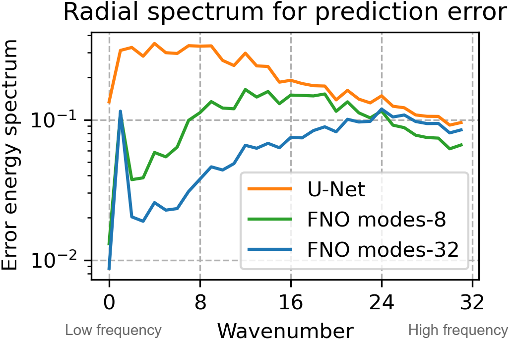
Figure 1: Radial energy spectrum for prediction errors on Navier-Stokes for viscosity 1e-5. Larger wavenumbers represent higher frequencies. Computation details for the radial energy spectrum are provided in Appendix A.

In this research, we first present empirical evidence from a spectral perspective regarding the reasons behind FNO’s superiority over CNNs: FNO’s capacity to capture low-frequency information significantly surpasses that of CNNs. This observation aligns with the design of FNO, which utilizes global Fourier filters, whereas CNNs rely on local filters. This finding originates from the spectral analysis (or Fourier analysis) of the prediction errors as illustrated in Figure 1. Employing spectral analysis is imperative, not only for comprehending PDE characteristics (Kolmogorov, 1991) but also for designing efficient numerical algorithms (Briggs et al., 2000; Shen et al., 2011).

Despite FNO’s exceptional ability to capture low frequencies in data, it faces challenges in effectively learning high-frequency information. The limitation stems mainly from the use of global Fourier filters. Moreover, FNO truncates high-frequency modes for each Fourier layer, further restricting its high-frequency performance. Consequently, FNO exhibits a notable bias toward low frequencies. As illustrated in Figure 1, FNO demonstrates larger errors in higher frequencies than in lower frequencies. Notably, FNO’s low-frequency bias is distinct from the typical low-frequency bias seen in regular neural networks, which is likely caused by using ReLU as the activation function (Rahaman et al., 2019; Xu, 2020).

In this work, we introduce spectral boosting (SpecBoost), an ensemble learning framework designed to enhance high-frequency information capture using multiple neural operators. In SpecBoost, following the regular training of an FNO, a second FNO is trained to predict the residual of the first FNO’s predictions. The motivation behind this is that FNO’s low-frequency bias can be alleviated when the low-frequency components in the target data are relatively smaller. Since the first FNO can sufficiently capture low-frequency information, the residual between its prediction and the target data primarily contains high-frequency information. By learning from this residual, the second FNO is compelled to focus on the high-frequency information overlooked by the first FNO.

With SpecBoost, the FNO ensemble demonstrates proficiency in capturing both low-frequency and high-frequency information from diverse PDE data. Interestingly, SpecBoost’s improvement is more significant on PDE data with negligible high-frequency information. This is because a solo FNO introduces unexpected noises into high-frequency spectrums, compromising simulation accuracies. In contrast, SpecBoost effectively mitigates these noises, resulting in nearly zero magnitudes in high-frequency spectrums. Numerical experiments across various PDE applications demonstrate the effectiveness of SpecBoost, with a 34% to 71% reduction in error when predicting the Navier-Stokes equation, a 48% to 61% reduction in error for predicting the Darcy flow equation, and an up to 40% reduction in error for PDE data compression and reconstruction.

Moreover, SpecBoost presents a memory-efficient solution for training deep neural operators. Instead of training one solo deep neural operator, training an ensemble of two neural operators, each with half of the layers, costs less memory and provides improved accuracy without additional time consumption.

Contributions:

• By utilizing spectral analysis on the prediction error, we empirically explain FNO’s superiority over CNN. Specifically, FNO is more capable of learning low frequencies from intricate PDE data.

• To address the solo FNO’s limitation of low-frequency bias, we propose the SpecBoost framework, which effectively and efficiently captures high-frequency information, leading to notable accuracy improvements on various PDE tasks.

• We validate SpecBoost’s superiority over a solo FNO on various PDE applications, with an up to 71% error reduction.

2 Preliminary

Fourier Neural Operator (FNO) is designed to capture the mapping between a continuous input function $\mathcal{X}$ and its corresponding continuous output function $\mathcal{Y}$ in Fourier space. To conduct end-to-end training on FNO, function pair $(\mathcal{X},\mathcal{Y})$ are discretized to instance pair $(x,y)$ during the training process. The objective is to learn a mapping $\mathcal{G}$ between $(x,y)$, denoted as:

$$y=\mathcal{G}(x),$$ (1)

The mapping $\mathcal{G}$ involves the sequential steps of lifting the input channel using $\mathcal{P}$, conducting the mapping through $L$ Fourier layers $\{\mathcal{H}_{1},\mathcal{H}_{2},\dots,\mathcal{H}_{L}\}$, and then projecting back to the original channel through $\mathcal{Q}$:

$$\mathcal{G}=\mathcal{Q}\circ\mathcal{H}_{L}\circ\cdots\circ\mathcal{H}_{2}\circ\mathcal{H}_{1}\circ\mathcal{P}.$$ (2)

$\mathcal{P}$ and $\mathcal{Q}$ are pixel-wise transformations that can be implemented using models like Multilayer perceptron (MLP). Figure 2 illustrates the overall structure of FNO.

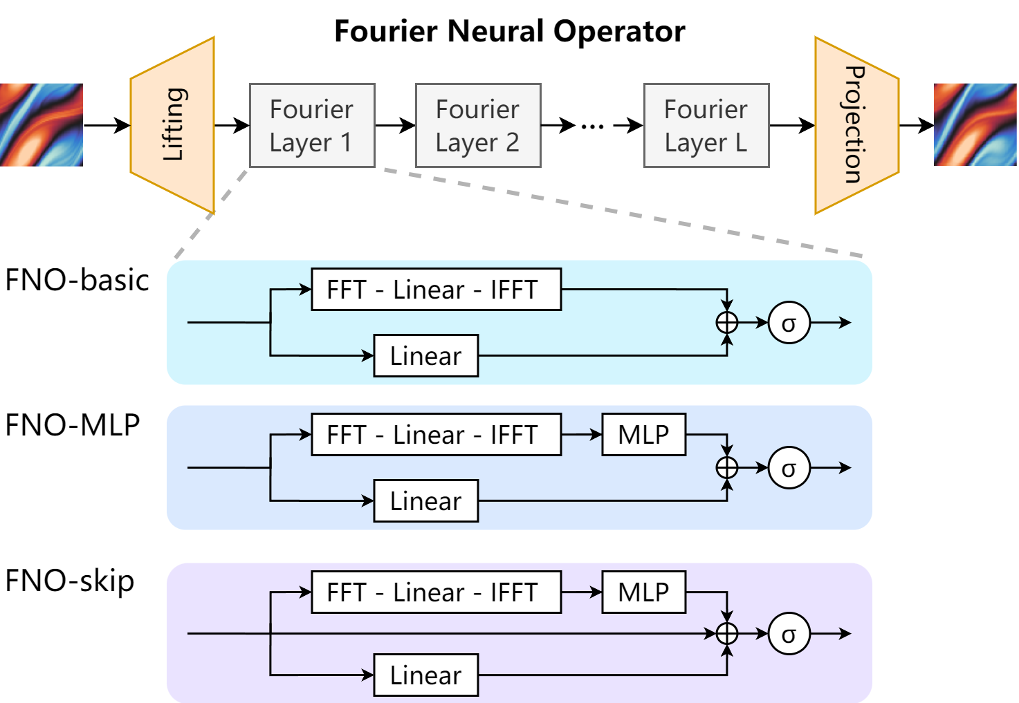
Figure 2: FNO architecture and designs for Fourier layers.

The key architecture of FNO is centred around its Fourier layer, illustrated in Figure 2. Fourier layer typically consists of a pixel-wise linear transformation with weight $W$ and bias $b$, and an integral kernel operator $\mathcal{K}$ (Li et al., 2021):

$$\mathcal{H}^{basic}(x)=\sigma\left(Wx+b+\mathcal{K}(x)\right),$$ (3)

with $\sigma$ as the nonlinear activation function. The integral kernel operator $\mathcal{K}$ undergoes a sequential process involving three operations: Fast Fourier Transformation (FFT) (Cochran et al., 1967), spectral linear transformation, and inverse FFT. The primary parameters of FNO are located in the spectral linear transformation. Hence, to avoid introducing extensive parameters, FNO truncates high-frequency modes in each Fourier layer. These truncated frequency modes can encompass rich spectrum information, especially for high-resolution inputs.

The authors of (Li et al., 2021) have also introduced alternative configurations for Fourier layers in their publicly available code. One adjustment involves incorporating a pixel-wise MLP, denoted as $\mathcal{M}$, after the kernel operator $\mathcal{K}$:

$$\mathcal{H}^{MLP}(x)=\sigma\left(Wx+b+\mathcal{M}(\mathcal{K}(x))\right).$$ (4)

Another modification to FNO involves including skip connections, which are commonly employed in training deep CNNs (He et al., 2016):

$$\mathcal{H}^{skip}(x)=\sigma\left(x+Wx+b+\mathcal{M}(\mathcal{K}(x))\right).$$ (5)

It’s shown that employing skip connections to Fourier layers enables the training of a deeper FNO (Tran et al., 2023).

Given the training dataset $\mathcal{D}=\{(x,y)\}$, the training objective is to minimize the relative mean square error (R-MSE), which is defined as:

$$\text{R-MSE}=\frac{1}{|\mathcal{D}|}\sum_{(x,y)\in\mathcal{D}}\frac{||\hat{y}-y||_{2}}{||y||_{2}},\ \hat{y}=\mathcal{G}(x),$$ (6)

where $||\cdot||_{2}$ represents the L2-norm.

3 Methodology

In this section, we begin with a spectral analysis of FNO in Section 3.1 to explain its superiority over CNNs and showcase its low-frequency bias. Following that, in Section 3.2, we introduce SpecBoost, an ensemble learning framework that exploits FNO’s low-frequency bias to enhance its ability to capture high-frequency information.

3.1 Spectral Analysis on FNO

In this section, we utilize spectral analysis to explore why FNO outperforms CNNs in solving PDEs. Specifically, we empirically demonstrate FNO’s significant proficiency in capturing low frequencies from PDE data compared to CNNs.

Consider solving the Navier-Stokes equation as an example. The Navier-Stokes equation serves as the fundamental PDE that models fluid dynamics. Fluid flow typically encompasses phenomena taking place at various scales, and accurately capturing these multiscale features is essential for precise predictions and a comprehensive understanding of intricate fluid behaviours. This section employs the dataset (Li et al., 2021) with a small viscosity of 1e-5, chosen for its intricate flow fields that are rich in high-frequency information. More details of the dataset are provided in Appendix B.1.

We choose U-Net (Ronneberger et al., 2015) as the representative CNN due to its efficacy in capturing both local and global features through the spatial downsampling pass in its architecture. Additionally, it serves as a widely used baseline in neural operator research (Li et al., 2021; Gupta & Brandstetter, 2022; Helwig et al., 2023). We chose the FNO model with truncating frequency modes of 8 and 32. FNO with 8 frequency modes keeps only the 8 lowest frequency components, whereas FNO with 32 frequency modes preserves almost all spectral information, given the input data resolution of 64 $\times$ 64. We train both U-Net and FNO models, utilizing the current flow field to predict the subsequent flow field in the sequence from the Navier-Stokes dataset.

We employ the radial energy spectrum to illustrate how energy is distributed in both the prediction and prediction error across low to high frequencies. Appendix A provides specifics on computing the radial energy spectrum. The energy in the Fourier domain is the sum of the squares of the Fourier magnitudes. According to Parseval’s theorem, the energy of a signal remains conserved during the discrete Fourier transform. Hence, when presenting prediction errors using the radial energy spectrum, the area beneath the spectrum curve is approximately identical to the mean square error (MSE) of the predictions with proper scaling.

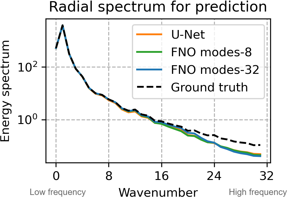
Figure 3: Radial energy spectrum for predictions and ground truth on Navier-Stokes for viscosity 1e-5. Larger wavenumbers represent higher frequencies. Details about radial energy spectrum are in Appendix A.

In Figure 3, we showcase the radial spectrum of predictions from U-Net and FNOs across all testing samples in the Navier-Stokes dataset. All models capture the overall radial spectrum of the ground truth, consistent with previous findings (Kovachki et al., 2021). For a more in-depth analysis of spectral performance, we present the radial spectrum of prediction errors from U-Net and FNOs in Figure 1. FNO shows substantially smaller low-frequency errors compared to U-Net, aligning with FNO’s use of global Fourier filters, while U-Net employs local filters. However, as frequencies shift from low to high, the superiority of FNO over U-Net diminishes, with almost no improvement observed when the wavenumber exceeds 24. In addition, FNO with a frequency mode of 32 exhibits lower errors than FNO with a frequency mode of 8. This emphasizes that truncating high-frequency modes can hinder the model’s capability to learn high-frequency information. In summary, the spectral analysis of prediction errors demonstrates FNO’s bias towards low frequencies while also revealing its limitation in capturing high-frequency information.

3.2 SpecBoost

Building upon FNO’s low-frequency bias, we suggest that mitigating FNO’s high-frequency errors could further improve its overall performance. To achieve this, we introduce SpecBoost, an ensemble learning framework that sequentially trains multiple FNOs. FNO’s low-frequency bias allows a solo FNO to capture low frequencies effectively, leaving its prediction residuals with rich high-frequency information. Leveraging a secondary FNO to learn from these residuals will enable us to preserve the high-frequency information overlooked by the first FNO.

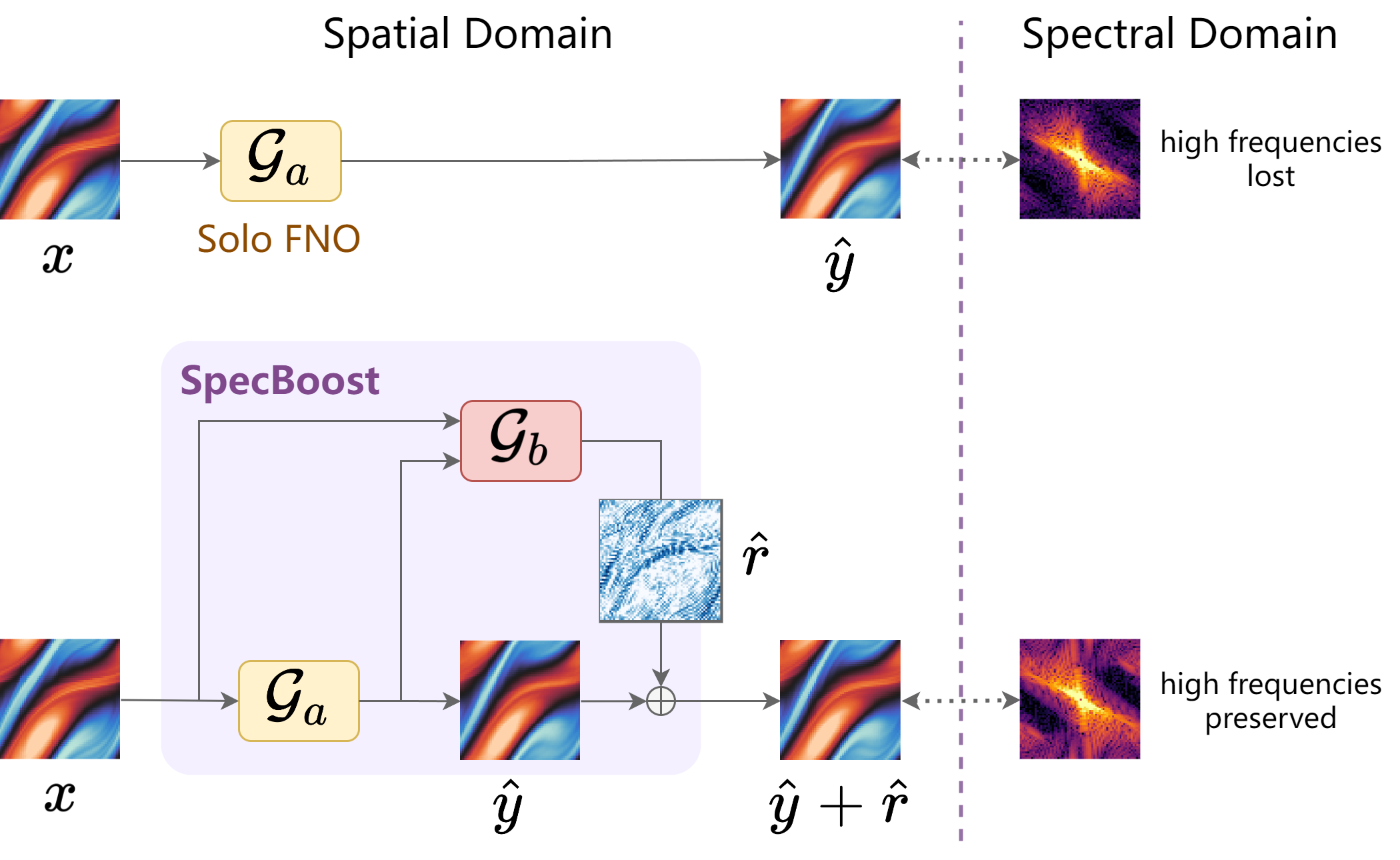
Figure 4: Illustration of the SpecBoost framework vs. a solo FNO.

Figure 4 illustrates the SpecBoost framework. The first FNO $\mathcal{G}_{a}$ undergoes standard training following Eqn. (6). For each training instance pair $(x,y)$, we calculate the prediction $\hat{y}=\mathcal{G}_{a}(x)$ and the corresponding residual $r=y-\hat{y}$ to build the residual dataset $\mathcal{D}_{r}=\{[x,\hat{y}],r\}$. Following this, the second FNO $\mathcal{G}_{b}$ is trained on the residual dataset $\mathcal{D}_{r}$ to predict the corresponding residual $r$, denoted as

$$\hat{r}=\mathcal{G}_{b}([x,\hat{y}]).$$ (7)

Note that [ , ] stands for concatenation operation on the channel level. Both $x$ and $\hat{y}$ are used as inputs to $\mathcal{G}_{b}$ to ensure sufficient information is provided for predicting the residual $r$. Hence, the input channel of the second FNO $\mathcal{G}_{b}$ is larger than that of the first FNO $\mathcal{G}_{a}$.

Once the two FNOs are trained, they can proceed with inference as one ensemble, shown in Figure 4. The predicted residual $\hat{r}$ from the second FNO $\mathcal{G}_{b}$ is added to the prediction $\hat{y}$ from the first FNO $\mathcal{G}_{a}$, yielding $\hat{y}+\hat{r}$ as the final output.

In general, the first FNO in SpecBoost captures the relatively lower frequencies in the data, while the second FNO focuses on capturing high-frequency details from the prediction residual of the first FNO.

Orthogonality of SpecBoost. A notable feature of the SpecBoost framework is that its sequential training process is orthogonal towards FNO variants. It doesn’t mandate a specific FNO structure or alternate its internal architecture. This property makes it compatible with a wide range of FNO variants, as well as traditional MLPs and CNNs. Moreover, by incorporating existing FNO variants, SpecBoost can handle diverse data formats, such as regular grids (Li et al., 2021), irregular grids (Liu et al., 2023), spherical coordinates (Bonev et al., 2023), cloud points (Li et al., 2023b), and general geometries (Li et al., 2023a; Serrano et al., 2023).

4 Experiments

Table 1: Relative error (%) comparison on Navier-Stokes between Solo and SpecBoost with U-Net and FNO variants. Imp. indicates the relative improvement from Solo to SpecBoost. All models employ autoregressive prediction with one-step input and one-step output data. The evaluation begins by taking the 10th data in the sequence as input, predicting the remaining sequence. The cumulative counts for autoregressive predictions at $\nu$ values of 1e-3, 1e-4, and 1e-5, $T$ are 40, 20, and 10, respectively.

Model	$\nu$ = 1e-3, $T$ = 50			$\nu$ = 1e-4, $T$ = 30			$\nu$ = 1e-5, $T$ = 20
	Solo	SpecBoost	Imp. (%)	Solo	SpecBoost	Imp. (%)	Solo	SpecBoost	Imp. (%)
U-Net	11.55 $\pm$ 4.73	2.73 $\pm$ 1.29	76.4	37.11 $\pm$ 0.27	35.05 $\pm$ 0.14	5.6	13.34 $\pm$ 0.58	11.64 $\pm$ 0.13	14.1
FNO-basic	1.38 $\pm$ 0.21	0.73 $\pm$ 0.12	47.1	22.75 $\pm$ 0.08	16.23 $\pm$ 2.28	28.7	8.02 $\pm$ 0.30	6.33 $\pm$ 0.51	21.1
FNO-MLP	0.68 $\pm$ 0.10	0.29 $\pm$ 0.04	57.4	11.19 $\pm$ 0.34	9.16 $\pm$ 0.73	18.1	6.51 $\pm$ 0.17	5.81 $\pm$ 0.20	10.8
FNO-skip	0.51 $\pm$ 0.02	0.15 $\pm$ 0.01	70.6	10.97 $\pm$ 0.34	7.26 $\pm$ 0.32	33.8	6.03 $\pm$ 0.05	3.51 $\pm$ 0.14	41.8

In this section, we conduct numerical experiments to validate the effectiveness of the SpecBoost method. Following previous work (Li et al., 2021; Kovachki et al., 2021), We evaluate SpecBoost’s performance on two PDE datasets: (i) the 2D incompressible Navier-Stokes equation for sequential prediction in Section 4.2 and (ii) the 2D steady-state Darcy flow equation for single-shot prediction in Section 4.3. We also investigate SpecBoost’s PDE data compression and reconstruction ability, utilizing an FNO-based superresolution model and an FNO-based autoencoder in Section 4.4. Moreover, In Section 4.5, we show that SpecBoost’s effectiveness is not due to the increased parameter count resulting from the ensemble of multiple FNOs; instead, it’s attributable to the sequential training approach. In Section 4.6, we demonstrate that SpecBoost’s spectral performance differs on PDEs with different levels of high-frequency information.

4.1 Experiment Description

Datasets. We evaluate the performance of SpecBoost on two broadly used datasets: (i) Navier-Stokes equation and (ii) Darcy flow equation. We detailedly introduce these two datasets in Appendix B.1.

Models. In our initial evaluation of the Navier-Stokes equation, we compare the U-Net and FNO variants outlined in Section 3.1. For all subsequent evaluations, we use FNO-skip as the representative of FNO due to its advantageous performance. Detailed hyperparameters for FNO are provided in Appendix B.2.

Solo vs. SpecBoost. For all evaluations, Solo denotes training a solo model, while SpecBoost represents training an ensemble of two models sequentially.

Metric. The employed evaluation metric aligns with previous work (Li et al., 2021; Tran et al., 2023), utilizing the R-MSE in Eqn. (6). For all evaluation results, we present the mean and standard deviation for each experiment across three random seeds.

4.2 Solving 2D Navier-Stokes Equation

Table 1 reports the performance of training a solo model and employing SpecBoost across U-Net and FNO variants for solving the Navier-Stokes equation. We follow the training and evaluation procedure as previous work suggested (Tran et al., 2023; Helwig et al., 2023).

As shown in Table 1, SpecBoost reduces the prediction error across all tested models for the Navier-Stokes equation. Among all models, the basic FNO model consistently outperforms U-Net, and the integration of MLP layers and skip connections further improves its performance. Besides, employing SpecBoost on FNO-skip yields optimal performance. Specifically, the relative prediction error for FNO-skip is reduced by 71%, 34%, and 42% for $\nu=$ 1e-3, 1e-4, and 1e-5 respectively. It’s worth noting that by exploiting FNO’s low-frequency bias, SpecBoost achieves these performance improvements without modifying FNO’s internal architecture. The experiment showcases the untapped potential of the FNO model, suggesting that with thoughtfully designed training, its performance can undergo substantial improvement.

4.3 Solving 2D Darcy Flow Equation

Table 2: Relative error ($1\times 10^{-3}$) comparison on Darcy flow between Solo and SpecBoost with FNO-skip. Imp. indicates the relative improvement from Solo to SpecBoost.

Method	$S$=85	$S$=141	$S$=211	$S$=421
Solo	9.46 $\pm$ 0.08	9.16 $\pm$ 0.10	9.19 $\pm$ 0.06	9.32 $\pm$ 0.10
SpecBoost	4.89 $\pm$ 0.04	4.00 $\pm$ 0.08	3.70 $\pm$ 0.04	3.65 $\pm$ 0.02
Imp. (%)	48.3	56.3	59.7	60.8

Table 2 evaluates the performance of SpecBoost on the steady-state Darcy flow equation across the dataset downsampled to various resolutions, denoted by $S$. Given the constraint of a relatively small training dataset (1800 samples), we augment the dataset through flipping and rotation. The model hyperparameters across diverse resolutions remain constant. We can make the following observations:

Firstly, in Table 2, SpecBoost consistently outperforms Solo across various resolutions, achieving an up to 61% reduction in error.

Secondly, as the resolution $S$ increases, Solo and SpecBoost behave differently. SpecBoost’s performance tends to increase with the resolution, while Solo maintains relatively stable. This disparity aligns with SpecBoost’s enhanced capacity to capture high-frequency information from the data. With increasing resolution, the low-frequency components in the data remain relatively stable while additional high-frequency details emerge. Solo cannot capture these additional high-frequency details, thereby showing minimal improvement as resolution increases.

Resolution invariance testing. Figure 5 examines the resolution-invariant property of both Solo and SpecBoost, as FNO is designed to be resolution-invariant. Figure 5 illustrates that optimal performance is achieved when training FNO on data with the same resolution as the testing data. Training on resolutions higher or lower than the testing data negatively impacts testing performance. SpecBoost’s improvements extend across various testing resolutions, with more significant enhancements observed at closer resolutions.

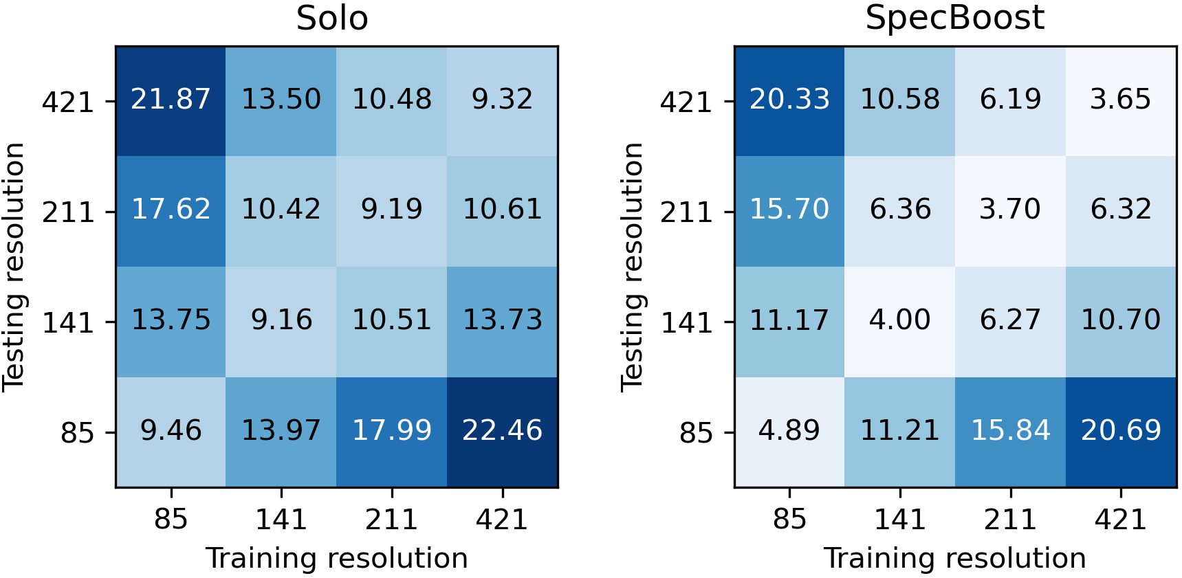
Figure 5: Relative error ($1\times 10^{-3}$) comparison on Darcy flow between Solo and SpecBoost with FNO-skip under distinct training and testing resolutions.

4.4 PDE Data Reconstruction

In addition to solving PDEs, we further explore SpecBoost’s effectiveness for PDE data compression and reconstruction. Compressing (Rowley & Dawson, 2017) and reconstructing (Fukami et al., 2019) PDE simulation data are pivotal in advancing fluid dynamics research. We assess the compression and reconstruction capabilities of SpecBoost on the 2D Navier-Stokes dataset with $\nu$ = 1e-5. The evaluation involves compressing the flow field to a lower resolution and reconstructing it to the original resolution, aiming to minimize the reconstruction error. We compare the following three methods: (i) Bicubic: compression and reconstruction of data using bicubic interpolation. (ii) FNO-SR: compression of data with bicubic interpolation, followed by reconstruction using an FNO-based superresolution model. (iii) FNO-AE: compression and reconstruction of data using an FNO-based autoencoder.

Convolutional layers are additionally stacked with the input layer or the output layer of the FNO to enable upsampling or downsampling. Details of the model architecture are provided in Appendix D.

Table 3: Relative error (%) comparison on Navier-Stokes ($\nu$=1e-5) data reconstruction between Solo and SpecBoost with FNO-SR and FNO-AE. Imp. indicates the relative improvement from Solo to SpecBoost. CR. indicates the data compression ratio.

CR.	Method	Bicubic	FNO-SR	FNO-AE
2 $:$ 1	Solo	2.70	4.98 $\pm$ 0.08	1.89 $\pm$ 0.06
	SpecBoost	-	4.28 $\pm$ 0.08	1.14 $\pm$ 0.03
	Imp. (%)	-	14.1	39.7
4 $:$ 1	Solo	4.78	2.70 $\pm$ 0.01	2.51 $\pm$ 0.05
	SpecBoost	-	1.56 $\pm$ 0.01	1.82 $\pm$ 0.07
	Imp. (%)	-	42.2	27.5
8 $:$ 1	Solo	7.51	3.90 $\pm$ 0.01	3.32 $\pm$ 0.09
	SpecBoost	-	2.98 $\pm$ 0.03	2.70 $\pm$ 0.04
	Imp. (%)	-	23.6	18.7
16 $:$ 1	Solo	11.54	5.21 $\pm$ 0.04	4.36 $\pm$ 0.08
	SpecBoost	-	4.82 $\pm$ 0.03	4.35 $\pm$ 0.08
	Imp. (%)	-	7.5	0.2

Table 3 reports the performance of different configurations on the N-S dataset. We can make the following three observations: To begin, SpecBoost consistently outperforms Solo in all scenarios, aligning with our findings from previous sections. Secondly, FNO-AE exhibits superior performance compared to FNO-SR. The ability of FNO-AE to learn a more effective representation surpasses Bicubic, which is the downsampling component when testing FNO-SR. Third, As the compression ratio increases, more information is lost during the compression. Hence, the performance of Solo and SpecBoost both decreases. Finally, as the compression ratio increases, the relative improvements of SpecBoost compared to Solo decrease, as high-frequency information is more likely to be discarded during compression. With less high-frequency information, the superiority of SpecBoost against Solo is less evident.

4.5 Ablation Study on Efficiency

Table 4: Relative error (%) comparison on Navier-Stokes ($\nu$=1e-5) between Solo, Dual, and SpecBoost with FNO-skip under the same number of total layers. Dual indicates jointly training an ensemble of two models, contrasting with the sequential training of SpecBoost. Mem. denotes the memory cost per training sample.

Method	Layers	Relative	Max Mem.	Total
		error (%)	(MB)	time (h)
Solo	4	6.97 $\pm$ 0.06	204	0.96
Dual	2+2	7.45 $\pm$ 0.10	201	1.02
SpecBoost	2+2	7.20 $\pm$ 0.02	188	1.03
Solo	8	6.03 $\pm$ 0.05	341	1.81
Dual	4+4	6.31 $\pm$ 0.02	323	1.88
SpecBoost	4+4	5.60 $\pm$ 0.04	264	1.92
Solo	16	5.94 $\pm$ 0.05	613	3.54
Dual	8+8	5.94 $\pm$ 0.04	564	3.61
SpecBoost	8+8	3.51 $\pm$ 0.14	400	3.63

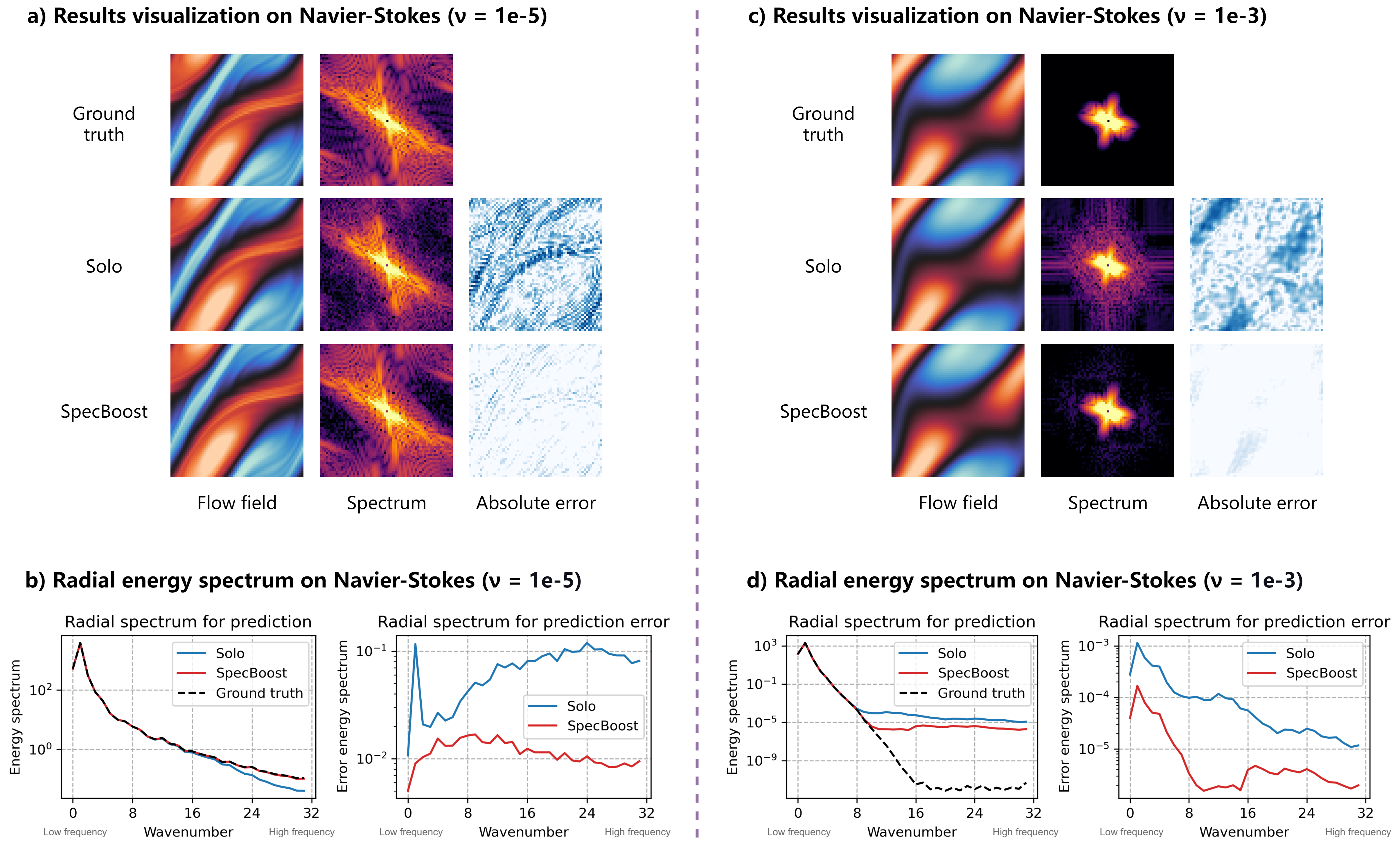
Figure 6: Comparision of spectral performance on Navier-Stokes between Solo and SpecBoost with FNO-skip. Details for radial energy spectrum are provided in Appendix A.

This section aims to answer whether SpecBoost enhances performance by making the model deeper with more parameters, as it ensembles two FNOs. The ablation study in Table 4 indicates that this is not the case. Table 4 compares different strategies for training the FNO-skip model on Navier-Stokes with $\nu$ = 1e-5.

To ensure a fair comparison, we configure candidate strategies to create models with identical layer numbers and nearly equivalent parameter counts. For example, for models with a total of 16 layers, we compare a solo 16-layer FNO-skip model, namely Solo in Table 4, with an ensemble of two 8-layer models trained iteratively with SpecBoost. Additionally, to account for the additional skip connections introduced by the ensemble model across multiple layers, which are absent in the solo 16-layer model, we train a model with the same structure as the ensemble, named Dual in Table 4. All models share the same hyperparameters besides the layer.

The results reveal that, with relatively deeper models, i.e., 8 and 16 layers, the sequentially trained model demonstrates lower errors compared to the model trained as a whole. Nevertheless, when the total layers are limited to 4, SpecBoost exhibits poorer performance. This is attributed to the detrimental effects of employing an overly shallow two-layer FNO surpassing the positive impact of Specboost. This emphasizes the need to avoid excessively weak submodels within the ensemble.

Memory efficient training. When assessing memory usage during FNO training, SpecBoost stands out as a memory-efficient solution, as iteratively training half-depth models require less memory. Specifically, with a total of 16 layers, SpecBoost achieves a 35% reduction in maximum memory consumption, measured per instance, with almost negligible additional time cost. Such a feature enables SpecBoost to train larger neural operators with limited memory.

4.6 Spectral Analysis on SpecBoost

In this section, we present the spectral analysis of SpecBoost to further investigate its properties. Specifically, we show the 2D spectrums and radial energy spectrums for the prediction results. We analyze the Navier-Stokes equation with $\nu=$ 1e-5 and 1e-3, representing PDE datasets with rich and minimal high-frequency details.

Spectral analysis on PDE rich in high frequencies. Examining the 2D spectrum in Figure 6 (a) reveals that training Solo leads to a loss of high-frequency details in the ground truth data. SpecBoost, however, effectively captures these high-frequency details, yielding a markedly diminished prediction residual.

The radial energy spectrums of the prediction residuals, shown in Figure 6 (b), further confirm SpecBoost’s success in reducing high-frequency residuals. For higher wave numbers, the SpecBoost lowers the residual energy by nearly a degree of magnitude. In conclusion, SpecBoost effectively captures the high-frequency details often overlooked when training Solo, thereby augmenting overall accuracy.

Spectral analysis on PDE lacking high frequencies. The 2D spectrum of ground truth in Figure 6 (c) indicates that the flow field with $\nu$ = 1e-3 exhibits minimal high-frequency details. Notably, the enhancement of SpecBoost on low-frequency PDEs partly differs from its enhancement on high-frequency PDEs. SpecBoost is beneficial in mitigating the high-frequency noises introduced by training a solo model. These high-frequency noises are visually apparent in the 2D spectrum presented in Figure 6 (c). In essence, such high-frequency noises still stem from the low-frequency bias. The low-frequency bias doesn’t imply zero magnitudes in high-frequency predictions; rather, it indicates a lack of precision in high-frequency predictions.

The radial energy spectrum of low-frequency PDEs in Figure 6 (d) reveals a distinct pattern compared to that of high-frequency PDEs. When employing Solo, the high-frequency residual is relatively smaller than the low-frequency residual, given that the nearly empty high-frequency components are easier to learn. SpecBoost contributes to a decrease in both high-frequency and low-frequency residuals. In the context of low-frequency PDEs, SpecBoost primarily operates to denoise the spectrum and confine the high-frequency components.

Error accumulation. Due to the distinct spectral behaviours of SpecBoost in high-frequency and low-frequency PDEs, its influence on error accumulation differs, as illustrated in Figure 7. On the dataset with rich high-frequency details, the enhancement provided by SpecBoost tends to diminish as error accumulates. This phenomenon is attributed to the fact that long-term prediction error is more closely tied to the low-frequency components in the data (Davidson, 2015), and SpecBoost’s improvement in low-frequency accuracy is limited when $\nu$ = 1e-5. Conversely, for low-frequency PDEs, SpecBoost reduces both low-frequency and high-frequency residuals, resulting in an improvement conducive to long-term prediction.

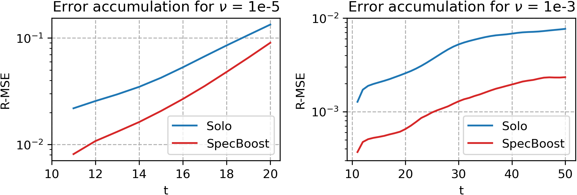
Figure 7: Relative error (%) accumulation comparison on Navier-Stokes between Solo and SpecBoost with FNO-skip. t denotes the sequential index in the Navier-Stokes dataset.

5 Related Work

5.1 Neural Operators for Solving PDEs

Recognized for their exceptional approximation capabilities, neural networks have emerged as a promising tool for tackling PDEs. Physics-Informed Neural Networks (PINNs) (Raissi et al., 2019) leverage neural networks to fit the PDE solutions in a temporal and spatial range while adhering to PDE constraints. On the other hand, the operator learning paradigm, such as DeepONet (Lu et al., 2021a), neural operators (Li et al., 2021; Kovachki et al., 2021), and message passing neural PDE solvers (Brandstetter et al., 2022), offers an alternative approach by employing neural networks to fit the complex operators for solving PDEs, directly mapping input functions to their target functions.

Among the neural operators, FNO (Li et al., 2021) incorporates the Fast Fourier Transform (FFT) (Cochran et al., 1967) in its network architecture, achieving both advantageous efficiency and prediction accuracy. As a resolution-invariant model, FNO trained on low-resolution data can be directly applied to infer on high-resolution data. Notable efforts have been made to enhance the performance of FNO from various aspects (Tran et al., 2023; Poli et al., 2022; Rahman et al., 2022; Gupta & Brandstetter, 2022; Saad et al., 2023; Brandstetter et al., 2023; Helwig et al., 2023; Wang et al., 2024). Several studies aim to improve FNO’s effectiveness in solving PDEs with distinctive properties, including coupled PDEs (Xiao et al., 2023), inverse problems for PDEs (Molinaro et al., 2023), and steady-state PDEs (Marwah et al., 2023). Since FNO relies on Fourier transform on regular meshed grids, broad work focuses on enabling FNO to process various data formats, including irregular grids (Liu et al., 2023), spherical coordinates (Bonev et al., 2023), cloud points (Li et al., 2023b), and general geometries (Li et al., 2023a; Serrano et al., 2023).

In this work, the proposed SpecBoost framework doesn’t involve altering the internal architecture of neural operators. Consequently, SpecBoost is orthogonal to most existing methods, as it imposes no requirements on the model architecture or data formats.

5.2 Spectral Properties for Neural Networks

Low-frequency bias. It has been observed that during the training process, neural networks employing the ReLU activation function tend to first learn low frequencies in data and progress more slowly in learning high frequencies (Rahaman et al., 2019; Xu, 2020). This characteristic diverges from traditional numerical solvers, which typically converge on high frequencies first. The implications of this low-frequency bias have been investigated in PINN research (Karniadakis et al., 2021; Lu et al., 2021b). PINNs inherit the low-frequency bias from neural networks and face limitations in accurately capturing high frequencies within PDEs (Markidis, 2021).

In this work, we showcase a unique low-frequency bias in FNO, primarily attributed to the use of global Fourier filters and the truncation of high-frequency modes. This characteristic distinguishes FNO’s low-frequency bias from the typical low-frequency bias observed in regular neural networks. Consequently, specialized methods are needed to address this particular limitation.

Fourier feature and Fourier transform. Research in computer vision has indicated that integrating Fourier features into neural network inputs expedites the convergence of high frequencies (Tancik et al., 2020; Mildenhall et al., 2021). In PINN, the Fourier features have been explored as a strategy to mitigate the impact of low-frequency preference (Karniadakis et al., 2021). We’d like to underscore that the application of Fourier features differs fundamentally from the Fourier transform in FNO. Fourier features elevate input features to more discernible high-dimensional representations using their Fourier series, thereby augmenting the high-frequency performance of neural networks. No Fourier transform is applied directly across the input features. Conversely, FNO employs FFT to capture spatial relations among input features.

6 Conclusion

This study provides empirical evidence from a spectral perspective to elucidate the superior performance of FNO over CNNs. The pivotal factor lies in FNO’s exceptional capability to capture low-frequency information. Building on this insight, we introduce SpecBoost as a solution to mitigate the low-frequency bias in FNO caused by global Fourier filters. The results across different PDE tasks underscore the efficacy and efficiency of the SpecBoost framework.

Limitation and Future Work. Our work is only tested with PDE datasets on regular grids. For future work, we aim to explore SpecBoost across a broader scope of PDE data formats. Given FNO’s distinctive spectral properties compared to numerical solvers, we’re also interested in comprehending the spectral properties of hybrid methods.

Appendix A Radial Energy Spectrum

Here, we provide the process to compute the radial energy spectrums in Figure 1, Figure 3, and Figure 6. To maintain the total energy, the radial energy spectrum employed in this work differs from the commonly used radial averaged energy spectrum.

• Compute the 2D Fourier transform. Use the Fast Fourier Transform (FFT) to transform the input 2D matrix from the spatial domain to the frequency domain.

• Compute the wave numbers. For each entry in the Fourier-transformed matrix, compute its wave number, which is the distance of that entry from the center of the Fourier-transformed matrix.

• Bin the wave numbers. Divide the wave numbers into bins. Each bin represents a range of wave numbers. For the 64 $\times$ 64 matrix, we set 32 bins, each with a range of 1.

• Compute energy in each bin. For each bin, sum the squared magnitudes of the Fourier coefficients that fall within the corresponding wave number range. This sum represents the energy in that frequency range.

The radial energy spectrum redistributes the energy of the 2D spectrum radially, resulting in a clearer visualization.

Appendix B Experimental Setup

B.1 Datasets

Navier-Stokes equation. As a fundamental PDE in fluid dynamics, the Navier-Stokes equation finds significance in diverse applications, including weather forecasting and aerospace engineering. Here, we consider the 2D incompressible Navier-Stokes dataset for viscosity following (Li et al., 2021):

$$\partial_{t}w(x,t)+u(x,t)\cdot\nabla w(x,t) =\nu\Delta w(x,t)+f(x),$$ (8)

$$\nabla\cdot u(x,t) =0,$$

$$w(x,0) =w_{0}(x).$$

The equation involves the viscosity field $w(x,t)\in\mathbb{R}$, with an initial value of $w_{0}(x)$, while $u\in\mathbb{R}^{2}$ represents the velocity field. The solution domain spans $x\in(0,1)^{2}$, $t\in\{1,2,\dots,T\}$. The forcing function is represented by $f(x)$. The viscosity coefficient, $\nu$, quantifies a fluid’s resistance to deformation or flow. The dataset comprises experiments with three viscosity coefficients: $\nu$ = 1e-3, 1e-4, and 1e-5, corresponding to sequence lengths $T$ of 50, 30, and 20, respectively. For smaller $\nu$ values, the flow field exhibits increased chaos and contains more high-frequency information.

The prediction task involves using the initial ten viscosity fields in the sequence to predict the remaining ones. The viscosity field resolution is 64 $\times$ 64. For all viscosities, we use 1000 sequences for training and 200 for testing. No data augmentation approach is applied.

Darcy flow equation. Consider the 2D steady-state Darcy Flow equation following (Li et al., 2021):

$$-\nabla\cdot(a(x)\nabla u(x)) =f(x), x\in(0,1)^{2}$$ (9)

$$u(x) =0, x\in\partial(0,1)^{2}$$

where $a(x)$ is the diffusion coefficient and $f(x)$ is the forcing function. The goal is to use coefficient $a(x)$ to predict the solution $u(x)$ directly. The dataset includes diffusion coefficients and corresponding solutions at a resolution of 421 $\times$ 421. Datasets at smaller resolutions are derived through downsampling.

A total of 2048 samples are provided. We use 1800 samples for training and 248 for testing. Training data is augmented through flipping and rotations at 90, 180, and 270 degrees.

B.2 Hyperparameter Settings

This section focuses on the hyperparameters used in our experiments for FNOs, including layers, frequency modes, and hidden channels. These hyperparameters remain identical across FNO-basic, FNO-MLP, and FNO-skip.

Navier-Stokes experiment in Table 1, Figure 1, Figure 3, Figure 6, and Figure 7:

• $\nu$ = 1e-3: layers: 8, frequency modes: 16, hidden channels: 60.

• $\nu$ = 1e-4: layers: 8, frequency modes: 16, hidden channels: 100.

• $\nu$ = 1e-5: layers: 8, frequency modes: 32, hidden channels: 100.

Ablation study in Table 4: frequency modes: 32, hidden channels: 100.

Darcy flow experiment in Table 2 and Figure 5: layers: 6, frequency modes: 24, hidden channels: 30.

Data reconstruction experiment in Table 3: layers: 8, frequency modes: 16, hidden channels: 30.

B.3 Hardware

All experiments are conducted on a Linux server with 8 Intel Xeon Gold 6154 cores, 64 GB memory and one Nvidia-V100 GPU-32GB with PCIe connections.

B.4 Code Implementation

We append the skeleton code repository in the appended file. Our model configurations are provided in previous sections. We will open-source the repository and ensure the reproducibility of our method upon acceptance.

Appendix C Ablation Study on SpecBoost over Different FNO Configurations

In this section, we conduct an ablation study on the effectiveness of SpecBoost over different FNO configurations. We config FNO with two key hyperparameters of FNO, namely layers and frequency modes, on Navier-Stokes datasets with $\nu$ = 1e-3 and $\nu$ = 1e-5. The results on shown in Table 5 and Table 6 respectively.

Table 5: Relative error (%) comparison on Navier-Stokes ($\nu$ = 1e-3) between Solo and SpecBoost utilizing FNO-skip with different layers and frequency modes. The hidden channels of FNO-skip are set to 60. Imp. indicates the relative improvement from Solo to SpecBoost.

Layer	modes = 8			modes = 16			modes = 32
	Solo	SpecBoost	Imp. (%)	Solo	SpecBoost	Imp. (%)	Solo	SpecBoost	Imp. (%)
4	0.47 $\pm$ 0.03	0.20 $\pm$ 0.01	57.1	1.73 $\pm$ 0.40	0.32 $\pm$ 0.07	81.3	1.91 $\pm$ 0.31	0.30 $\pm$ 0.02	84.1
8	0.39 $\pm$ 0.03	0.17 $\pm$ 0.01	55.1	0.47 $\pm$ 0.01	0.14 $\pm$ 0.01	69.7	0.45 $\pm$ 0.01	0.18 $\pm$ 0.02	59.5
16	0.40 $\pm$ 0.01	0.20 $\pm$ 0.01	49.1	0.46 $\pm$ 0.01	0.21 $\pm$ 0.02	54.8	0.41 $\pm$ 0.01	0.19 $\pm$ 0.02	52.5

Table 5 illustrates the impact of frequency modes and layers on Navier-Stokes with $\nu$ = 1e-3. Increasing frequency modes fails to enhance Solo and SpecBoost performance. This is because Navier-Stokes with $\nu$ = 1e-3 contains negligible high-frequency information. While increasing layers from 4 to 8 yields performance improvements for both Solo and SpecBoost, further increments to 16 don’t provide additional benefits, likely due to the risk of overfitting with deeper models.

Table 6: Relative error (%) comparison on Navier-Stokes ($\nu$ = 1e-5) between Solo and SpecBoost utilizing FNO-skip with different layers and frequency modes. The hidden channels of FNO-skip are set to 100. Imp. indicates the relative improvement from Solo to SpecBoost.

Layer	modes = 8			modes = 16			modes = 32
	Solo	SpecBoost	Imp. (%)	Solo	SpecBoost	Imp. (%)	Solo	SpecBoost	Imp. (%)
4	6.64 $\pm$ 0.03	6.21 $\pm$ 0.06	6.45	6.55 $\pm$ 0.10	4.84 $\pm$ 0.03	26.0	6.97 $\pm$ 0.06	5.60 $\pm$ 0.04	19.6
8	6.07 $\pm$ 0.03	5.73 $\pm$ 0.05	5.63	5.76 $\pm$ 0.04	3.92 $\pm$ 0.03	31.9	6.03 $\pm$ 0.05	3.51 $\pm$ 0.14	41.8
16	6.18 $\pm$ 0.07	6.01 $\pm$ 0.41	2.71	5.82 $\pm$ 0.13	4.08 $\pm$ 0.12	29.9	5.94 $\pm$ 0.05	3.64 $\pm$ 0.64	38.7

Table 6 illustrates the impact of frequency modes and layers on Navier-Stokes with $\nu$ = 1e-5. Notably, increasing frequency modes improves SpecBoost’s performance, whereas Solo remains unaffected. This disparity arises from SpecBoost’s ability to leverage higher frequency modes in Fourier layers, a benefit not accessible to Solo due to its low-frequency bias. Similarly to Table 5, while increasing layers from 4 to 8 yields performance improvements for both Solo and SpecBoost, further increments to 16 don’t provide additional benefits.

Appendix D FNO-based Superresolution (FNO-SR) Model and FNO-based Autoencoder (FNO-AE)

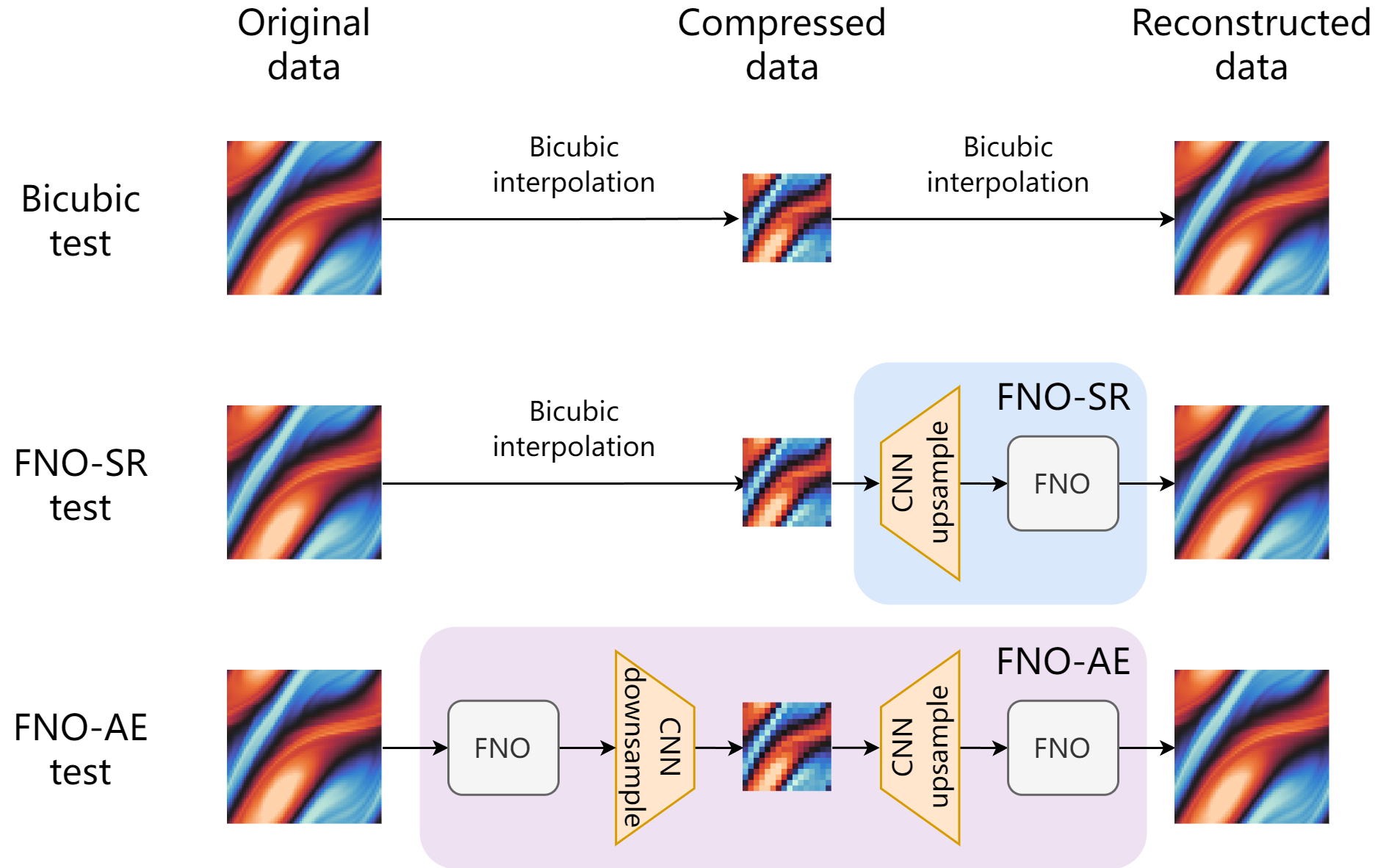
Figure 8: Illustration on data reconstruction experiment and architectures of FNO-SR and FNO-AE.

While FNO is crafted to be a resolution-invariant model, it always requires identical resolution for its input and output. As a result, FNO cannot take a low-resolution input to predict a high-resolution output or vice versa. To enable upsampling and downsampling for FNO, we integrate convolution layers into both the FNO-based superresolution model (FNO-SR) and the FNO-based autoencoder (FNO-AE), as illustrated in Figure 8.

FNO-SR and FNO-AE adopt a straightforward design, incorporating basic CNN layers for downsampling or upsampling. These layers are placed before the initial or after the final FNO layer, maintaining FNO’s internal architecture. The FNO-skip block is employed for both FNO-SR and FNO-AE.

In the experiment in Table 4, Solo means directly training a solo model. SpecBoost means sequentially training two models. In the case of SpecBoost applied to FNO-AE, two FNO-AEs generate two sets of latent variables, resulting in doubling the latent variable size. To ensure a fair comparison, the SpecBoost at a compression ratio of 2:1 is an ensemble of two FNO-AEs with a compression ratio of 4:1, for example.

Appendix E Detailed Darcy Flow Evaluations

We demonstrate the detailed results for Figure 5 in Table 7 and further include the improvement from Solo to SpecBoost. The experimental result indicates that the enhancements facilitated by SpecBoost can extend to close resolutions, with the magnitude of improvements diminishing as the resolution gap widens.

Table 7: Complete relative error ($1\times 10^{-3}$) comparison on Darcy flow between Solo and SpecBoost with FNO-skip. Imp. indicates the relative improvement from Solo to SpecBoost.

Train	Test: $S$=85			Test $S$=141			Test: $S$=211			Test: $S$=421
	Solo	SpecBoost	Imp. (%)	Solo	SpecBoost	Imp. (%)	Solo	SpecBoost	Imp. (%)	Solo	SpecBoost	Imp. (%)
$S$=85	9.46 $\pm$ 0.08	4.89 $\pm$ 0.04	48.3	13.75 $\pm$ 0.22	11.17 $\pm$ 0.17	18.8	17.62 $\pm$ 0.30	15.70 $\pm$ 0.27	10.9	21.87 $\pm$ 0.43	20.33 $\pm$ 0.33	7.0
$S$=141	13.97 $\pm$ 0.35	11.21 $\pm$ 0.22	19.8	9.16 $\pm$ 0.10	4.00 $\pm$ 0.08	56.3	10.42 $\pm$ 0.16	6.36 $\pm$ 0.05	39.0	13.50 $\pm$ 0.16	10.58 $\pm$ 0.16	21.6
$S$=211	17.99 $\pm$ 0.47	15.84 $\pm$ 0.24	12.0	10.51 $\pm$ 0.13	6.27 $\pm$ 0.05	40.3	9.19 $\pm$ 0.06	3.70 $\pm$ 0.04	59.7	10.48 $\pm$ 0.10	6.19 $\pm$ 0.05	40.9
$S$=421	22.46 $\pm$ 0.60	20.69 $\pm$ 0.29	7.9	13.73 $\pm$ 0.29	10.70 $\pm$ 0.18	22.1	10.61. $\pm$ 0.07	6.32 $\pm$ 0.13	40.4	9.32 $\pm$ 0.10	3.65 $\pm$ 0.02	60.8

Appendix F Visualization for Error Accumulation on Navier-Stokes

Since we employ autoregressive prediction with one-step input and one-step output on Navier-Stokes, the prediction error accumulates as the sequential index $t$ increases. We present the visualization of error accumulation in the experiment of Table 1 for Solo and SpecBoost with FNO-skip. The results for $\nu$ value at 1e-5, 1e-4, and 1e-3 are shown in Figure 9, 10, 11, respectively. We can observe that as the step $t$ increases, both Solo and SpecBoost accumulate prediction errors. Besides, SpecBoost constantly outperforms Solo, indicating its effectiveness during long-term prediction.

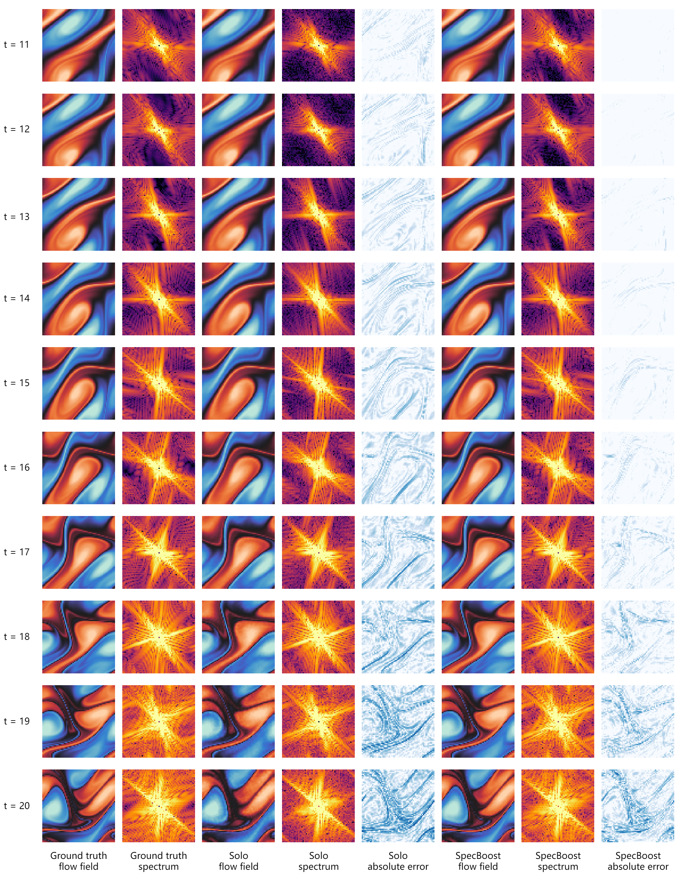
Figure 9: Visualization for error accumulation on Navier-Stokes ($\nu$ = 1e-5).

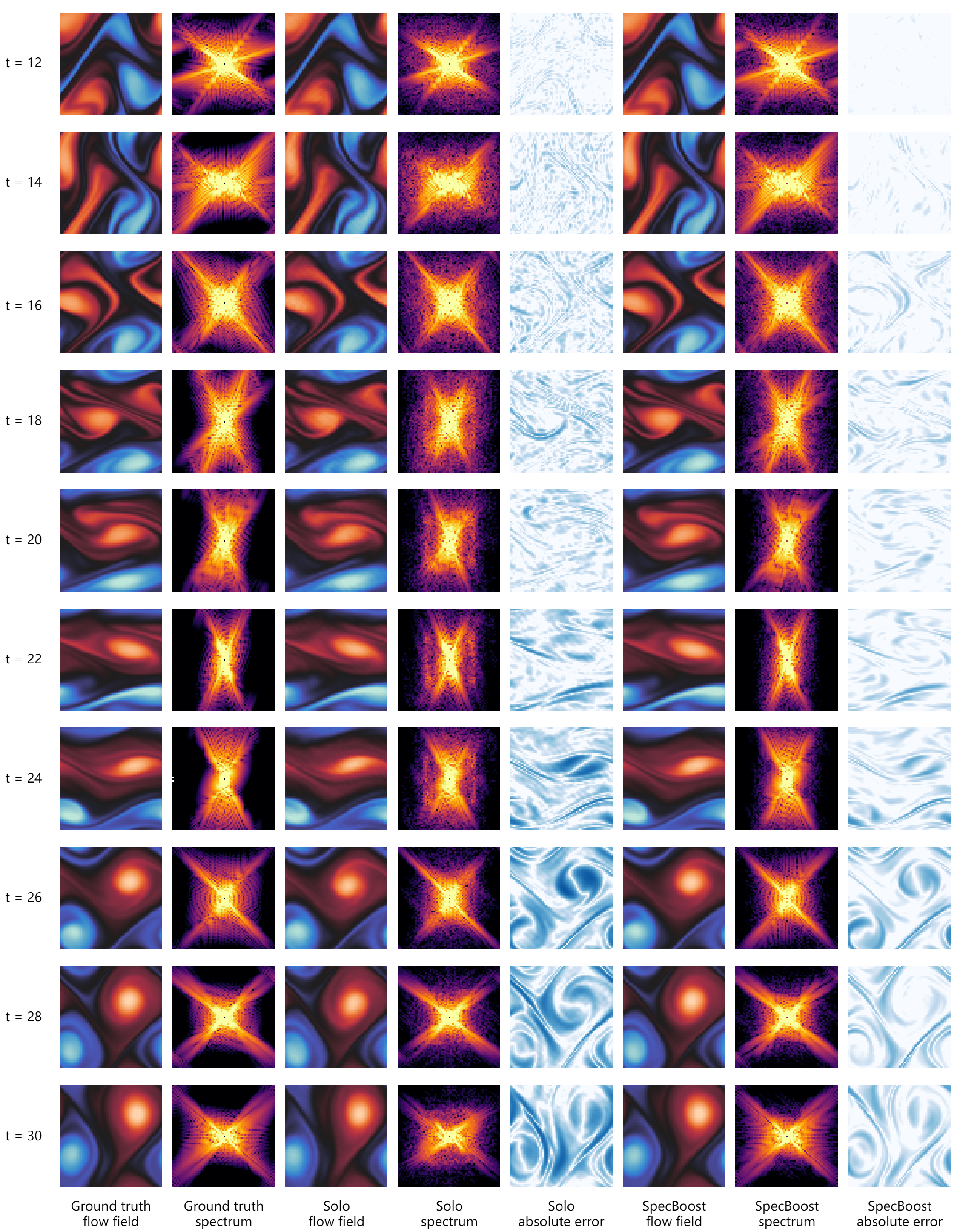
Figure 10: Visualization for error accumulation on Navier-Stokes ($\nu$ = 1e-4).

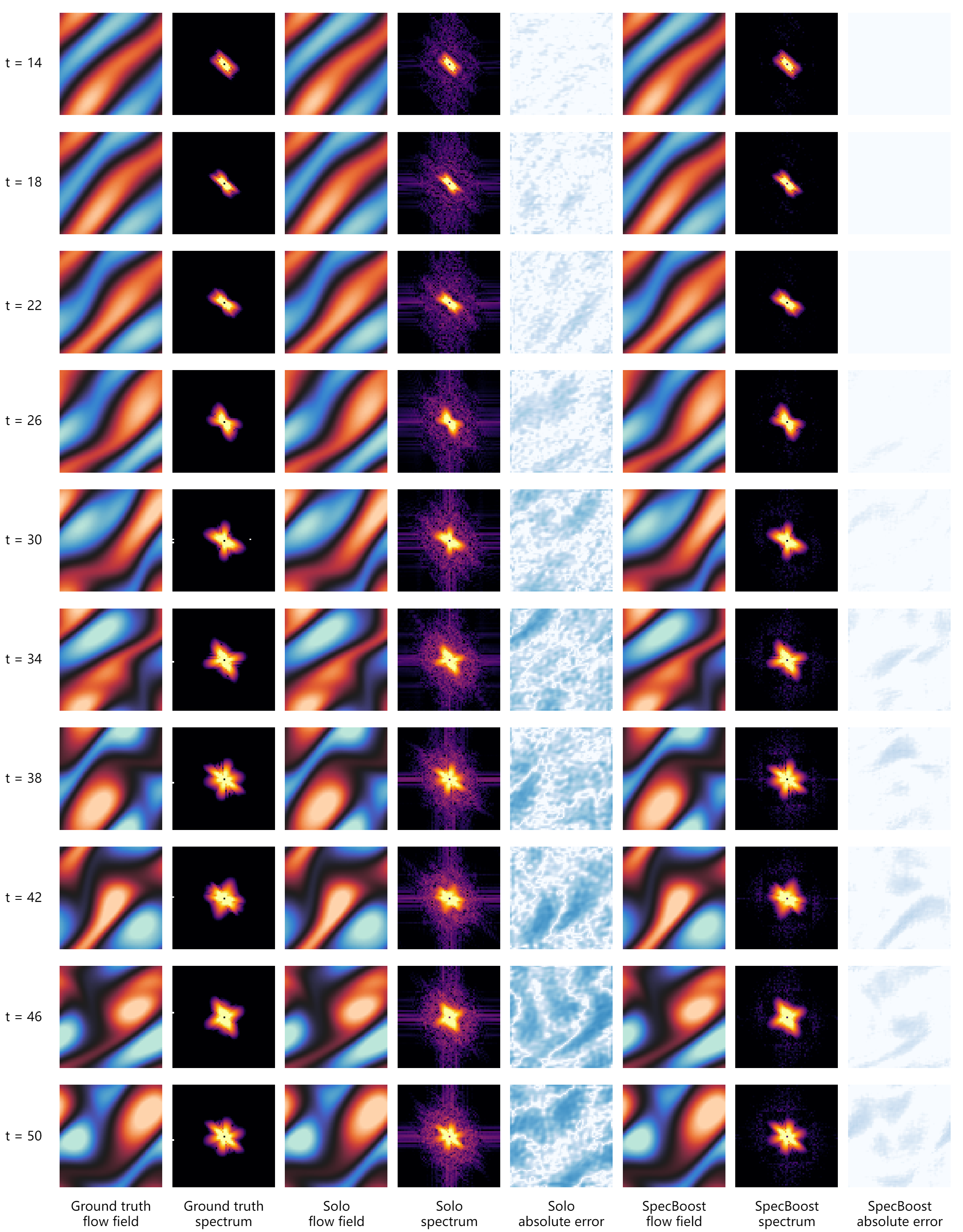
Figure 11: Visualization for error accumulation on Navier-Stokes ($\nu$ = 1e-3).

References

- Bonev et al. (2023) Bonev, B., Kurth, T., Hundt, C., Pathak, J., Baust, M., Kashinath, K., and Anandkumar, A. Spherical fourier neural operators: Learning stable dynamics on the sphere. In International Conference on Machine Learning, ICML 2023, 23-29 July 2023, Honolulu, Hawaii, USA, volume 202 of Proceedings of Machine Learning Research, pp. 2806–2823. PMLR, 2023. URL https://proceedings.mlr.press/v202/bonev23a.html.
- Brandstetter et al. (2022) Brandstetter, J., Worrall, D. E., and Welling, M. Message passing neural PDE solvers. In The Tenth International Conference on Learning Representations, ICLR 2022, Virtual Event, April 25-29, 2022. OpenReview.net, 2022. URL https://openreview.net/forum?id=vSix3HPYKSU.
- Brandstetter et al. (2023) Brandstetter, J., van den Berg, R., Welling, M., and Gupta, J. K. Clifford neural layers for PDE modeling. In The Eleventh International Conference on Learning Representations, ICLR 2023, Kigali, Rwanda, May 1-5, 2023. OpenReview.net, 2023. URL https://openreview.net/pdf?id=okwxL_c4x84.
- Briggs et al. (2000) Briggs, W. L., Henson, V. E., and McCormick, S. F. A multigrid tutorial. SIAM, 2000.
- Cochran et al. (1967) Cochran, W. T., Cooley, J. W., Favin, D. L., Helms, H. D., Kaenel, R. A., Lang, W. W., Maling, G. C., Nelson, D. E., Rader, C. M., and Welch, P. D. What is the fast fourier transform? Proceedings of the IEEE, 55(10):1664–1674, 1967.
- Davidson (2015) Davidson, P. A. Turbulence: an introduction for scientists and engineers. Oxford university press, 2015.
- Fukami et al. (2019) Fukami, K., Fukagata, K., and Taira, K. Super-resolution reconstruction of turbulent flows with machine learning. Journal of Fluid Mechanics, 870:106–120, 2019.
- Gupta & Brandstetter (2022) Gupta, J. K. and Brandstetter, J. Towards multi-spatiotemporal-scale generalized pde modeling. arXiv preprint arXiv:2209.15616, 2022.
- He et al. (2016) He, K., Zhang, X., Ren, S., and Sun, J. Deep residual learning for image recognition. In Proceedings of the IEEE conference on computer vision and pattern recognition, pp. 770–778, 2016.
- Helwig et al. (2023) Helwig, J., Zhang, X., Fu, C., Kurtin, J., Wojtowytsch, S., and Ji, S. Group equivariant fourier neural operators for partial differential equations. In International Conference on Machine Learning, ICML 2023, 23-29 July 2023, Honolulu, Hawaii, USA, volume 202 of Proceedings of Machine Learning Research, pp. 12907–12930. PMLR, 2023. URL https://proceedings.mlr.press/v202/helwig23a.html.
- Karniadakis et al. (2021) Karniadakis, G. E., Kevrekidis, I. G., Lu, L., Perdikaris, P., Wang, S., and Yang, L. Physics-informed machine learning. Nature Reviews Physics, 3(6):422–440, 2021.
- Kittel & Kroemer (1998) Kittel, C. and Kroemer, H. Thermal physics, 1998.
- Kolmogorov (1991) Kolmogorov, A. N. The local structure of turbulence in incompressible viscous fluid for very large reynolds numbers. Proceedings of the Royal Society of London. Series A: Mathematical and Physical Sciences, 434(1890):9–13, 1991.
- Kovachki et al. (2021) Kovachki, N. B., Li, Z., Liu, B., Azizzadenesheli, K., Bhattacharya, K., Stuart, A. M., and Anandkumar, A. Neural operator: Learning maps between function spaces. CoRR, abs/2108.08481, 2021.
- Li et al. (2021) Li, Z., Kovachki, N. B., Azizzadenesheli, K., Liu, B., Bhattacharya, K., Stuart, A. M., and Anandkumar, A. Fourier neural operator for parametric partial differential equations. In 9th International Conference on Learning Representations, ICLR 2021, Virtual Event, Austria, May 3-7, 2021. OpenReview.net, 2021. URL https://openreview.net/forum?id=c8P9NQVtmnO.
- Li et al. (2023a) Li, Z., Huang, D. Z., Liu, B., and Anandkumar, A. Fourier neural operator with learned deformations for pdes on general geometries. Journal of Machine Learning Research, 24(388):1–26, 2023a.
- Li et al. (2023b) Li, Z., Kovachki, N. B., Choy, C., Li, B., Kossaifi, J., Otta, S. P., Nabian, M. A., Stadler, M., Hundt, C., Azizzadenesheli, K., et al. Geometry-informed neural operator for large-scale 3d pdes. arXiv preprint arXiv:2309.00583, 2023b.
- Liu et al. (2023) Liu, N., Jafarzadeh, S., and Yu, Y. Domain agnostic fourier neural operators. arXiv preprint arXiv:2305.00478, 2023.
- Lu et al. (2021a) Lu, L., Jin, P., Pang, G., Zhang, Z., and Karniadakis, G. E. Learning nonlinear operators via deeponet based on the universal approximation theorem of operators. Nature machine intelligence, 3(3):218–229, 2021a.
- Lu et al. (2021b) Lu, L., Meng, X., Mao, Z., and Karniadakis, G. E. Deepxde: A deep learning library for solving differential equations. SIAM review, 63(1):208–228, 2021b.
- Markidis (2021) Markidis, S. The old and the new: Can physics-informed deep-learning replace traditional linear solvers? Frontiers in big Data, 4:669097, 2021.
- Marwah et al. (2023) Marwah, T., Pokle, A., Kolter, J. Z., Lipton, Z. C., Lu, J., and Risteski, A. Deep equilibrium based neural operators for steady-state pdes. arXiv preprint arXiv:2312.00234, 2023.
- Messiah (2014) Messiah, A. Quantum mechanics. Courier Corporation, 2014.
- Mildenhall et al. (2021) Mildenhall, B., Srinivasan, P. P., Tancik, M., Barron, J. T., Ramamoorthi, R., and Ng, R. Nerf: Representing scenes as neural radiance fields for view synthesis. Communications of the ACM, 65(1):99–106, 2021.
- Molinaro et al. (2023) Molinaro, R., Yang, Y., Engquist, B., and Mishra, S. Neural inverse operators for solving PDE inverse problems. In International Conference on Machine Learning, ICML 2023, 23-29 July 2023, Honolulu, Hawaii, USA, volume 202 of Proceedings of Machine Learning Research, pp. 25105–25139. PMLR, 2023. URL https://proceedings.mlr.press/v202/molinaro23a.html.
- Pathak et al. (2022) Pathak, J., Subramanian, S., Harrington, P., Raja, S., Chattopadhyay, A., Mardani, M., Kurth, T., Hall, D., Li, Z., Azizzadenesheli, K., et al. Fourcastnet: A global data-driven high-resolution weather model using adaptive fourier neural operators. arXiv preprint arXiv:2202.11214, 2022.
- Poli et al. (2022) Poli, M., Massaroli, S., Berto, F., Park, J., Dao, T., Ré, C., and Ermon, S. Transform once: Efficient operator learning in frequency domain. Advances in Neural Information Processing Systems, 35:7947–7959, 2022.
- Rahaman et al. (2019) Rahaman, N., Baratin, A., Arpit, D., Draxler, F., Lin, M., Hamprecht, F., Bengio, Y., and Courville, A. On the spectral bias of neural networks. In Chaudhuri, K. and Salakhutdinov, R. (eds.), Proceedings of the 36th International Conference on Machine Learning, volume 97 of Proceedings of Machine Learning Research, pp. 5301–5310. PMLR, 09–15 Jun 2019. URL https://proceedings.mlr.press/v97/rahaman19a.html.
- Rahman et al. (2022) Rahman, M. A., Ross, Z. E., and Azizzadenesheli, K. U-no: U-shaped neural operators. arXiv preprint arXiv:2204.11127, 2022.
- Raissi et al. (2019) Raissi, M., Perdikaris, P., and Karniadakis, G. E. Physics-informed neural networks: A deep learning framework for solving forward and inverse problems involving nonlinear partial differential equations. Journal of Computational physics, 378:686–707, 2019.
- Rashid et al. (2022) Rashid, M. M., Pittie, T., Chakraborty, S., and Krishnan, N. A. Learning the stress-strain fields in digital composites using fourier neural operator. Iscience, 25(11), 2022.
- Ronneberger et al. (2015) Ronneberger, O., Fischer, P., and Brox, T. U-net: Convolutional networks for biomedical image segmentation. In Medical Image Computing and Computer-Assisted Intervention–MICCAI 2015: 18th International Conference, Munich, Germany, October 5-9, 2015, Proceedings, Part III 18, pp. 234–241. Springer, 2015.
- Rowley & Dawson (2017) Rowley, C. W. and Dawson, S. T. Model reduction for flow analysis and control. Annual Review of Fluid Mechanics, 49:387–417, 2017.
- Saad et al. (2023) Saad, N., Gupta, G., Alizadeh, S., and Maddix, D. C. Guiding continuous operator learning through physics-based boundary constraints. In The Eleventh International Conference on Learning Representations, ICLR 2023, Kigali, Rwanda, May 1-5, 2023. OpenReview.net, 2023. URL https://openreview.net/pdf?id=gfWNItGOES6.
- Serrano et al. (2023) Serrano, L., Boudec, L. L., Koupaï, A. K., Wang, T. X., Yin, Y., Vittaut, J.-N., and Gallinari, P. Operator learning with neural fields: Tackling pdes on general geometries. arXiv preprint arXiv:2306.07266, 2023.
- Shen et al. (2011) Shen, J., Tang, T., and Wang, L.-L. Spectral methods: algorithms, analysis and applications, volume 41. Springer Science & Business Media, 2011.
- Tancik et al. (2020) Tancik, M., Srinivasan, P., Mildenhall, B., Fridovich-Keil, S., Raghavan, N., Singhal, U., Ramamoorthi, R., Barron, J., and Ng, R. Fourier features let networks learn high frequency functions in low dimensional domains. Advances in Neural Information Processing Systems, 33:7537–7547, 2020.
- Temam (2001) Temam, R. Navier-Stokes equations: theory and numerical analysis, volume 343. American Mathematical Soc., 2001.
- Tran et al. (2023) Tran, A., Mathews, A. P., Xie, L., and Ong, C. S. Factorized fourier neural operators. In The Eleventh International Conference on Learning Representations, ICLR 2023, Kigali, Rwanda, May 1-5, 2023. OpenReview.net, 2023. URL https://openreview.net/pdf?id=tmIiMPl4IPa.
- Wang et al. (2024) Wang, H., Li, J., Dwivedi, A., Hara, K., and Wu, T. Beno: Boundary-embedded neural operators for elliptic pdes. arXiv preprint arXiv:2401.09323, 2024.
- Xiao et al. (2023) Xiao, X., Cao, D., Yang, R., Gupta, G., Liu, G., Yin, C., Balan, R., and Bogdan, P. Coupled multiwavelet operator learning for coupled differential equations. In The Eleventh International Conference on Learning Representations, ICLR 2023, Kigali, Rwanda, May 1-5, 2023. OpenReview.net, 2023. URL https://openreview.net/pdf?id=kIo_C6QmMOM.
- Xu (2020) Xu, Z.-Q. J. Frequency principle: Fourier analysis sheds light on deep neural networks. Communications in Computational Physics, 28(5):1746–1767, June 2020. ISSN 1991-7120. doi: 10.4208/cicp.oa-2020-0085. URL http://dx.doi.org/10.4208/cicp.OA-2020-0085.
- Yang et al. (2021) Yang, Y., Gao, A. F., Castellanos, J. C., Ross, Z. E., Azizzadenesheli, K., and Clayton, R. W. Seismic wave propagation and inversion with neural operators. The Seismic Record, 1(3):126–134, 2021.