VN-EGNN: E(3)-Equivariant Graph Neural Networks with Virtual Nodes Enhance Protein Binding Site Identification

Abstract

Being able to identify regions within or around proteins, to which ligands can potentially bind, is an essential step to develop new drugs. Binding site identification methods can now profit from the availability of large amounts of 3D structures in protein structure databases or from AlphaFold predictions. Current binding site identification methods heavily rely on graph neural networks (GNNs), usually designed to output E($3$)-equivariant predictions. Such methods turned out to be very beneficial for physics-related tasks like binding energy or motion trajectory prediction. However, the performance of GNNs at binding site identification is still limited potentially due to the lack of dedicated nodes that model hidden geometric entities, such as binding pockets. In this work, we extend E($n$)-Equivariant Graph Neural Networks (EGNNs) by adding virtual nodes and applying an extended message passing scheme. The virtual nodes in these graphs are dedicated quantities to learn representations of binding sites, which leads to improved predictive performance. In our experiments, we show that our proposed method VN-EGNN sets a new state-of-the-art at locating binding site centers on COACH420, HOLO4K and PDBbind2020.

1 Introduction

Binding site identification remains a central computational problem in drug discovery. With the advent of AlphaFold (Jumper et al., 2021), millions of 3D structures of proteins have been unlocked for further investigation by the scientific community (Tunyasuvunakool et al., 2021; Cheng et al., 2023). Information about the 3D structure of a protein can provide crucial information about its function. One of the most important fields that should profit from these 3D structures, is drug discovery (Ren et al., 2023; Sadybekov & Katritch, 2023). It has been envisioned that the availability of 3D structures will allow to purposefully design drugs that alter protein function in a desired way. However, to enable structure-based drug design, further computational approaches have to be utilized/employed, concretely either docking or binding site identification methods (Lengauer & Rarey, 1996; Cheng et al., 2007; Halgren, 2009). While docking approaches predict the location of a specific small molecule, called ligand, within a protein’s active site upon binding, binding site identification aims at finding regions on the protein likely to form a binding pocket and interact with unknown ligands (Schmidtke & Barril, 2010). Note that docking and binding site identification are fundamentally different tasks in structure-based drug design: for the vast majority of proteins no ligand is known, and binding site identification methods can provide valuable information for understanding protein function, guiding rational drug design or identifying a protein as a potential drug target. For both approaches, deep learning methods, and specifically geometric deep learning have brought significant advances (Gainza et al., 2020; Sverrisson et al., 2021; Méndez-Lucio et al., 2021; Ganea et al., 2022; Stärk et al., 2022; Lu et al., 2022; Corso et al., 2023).

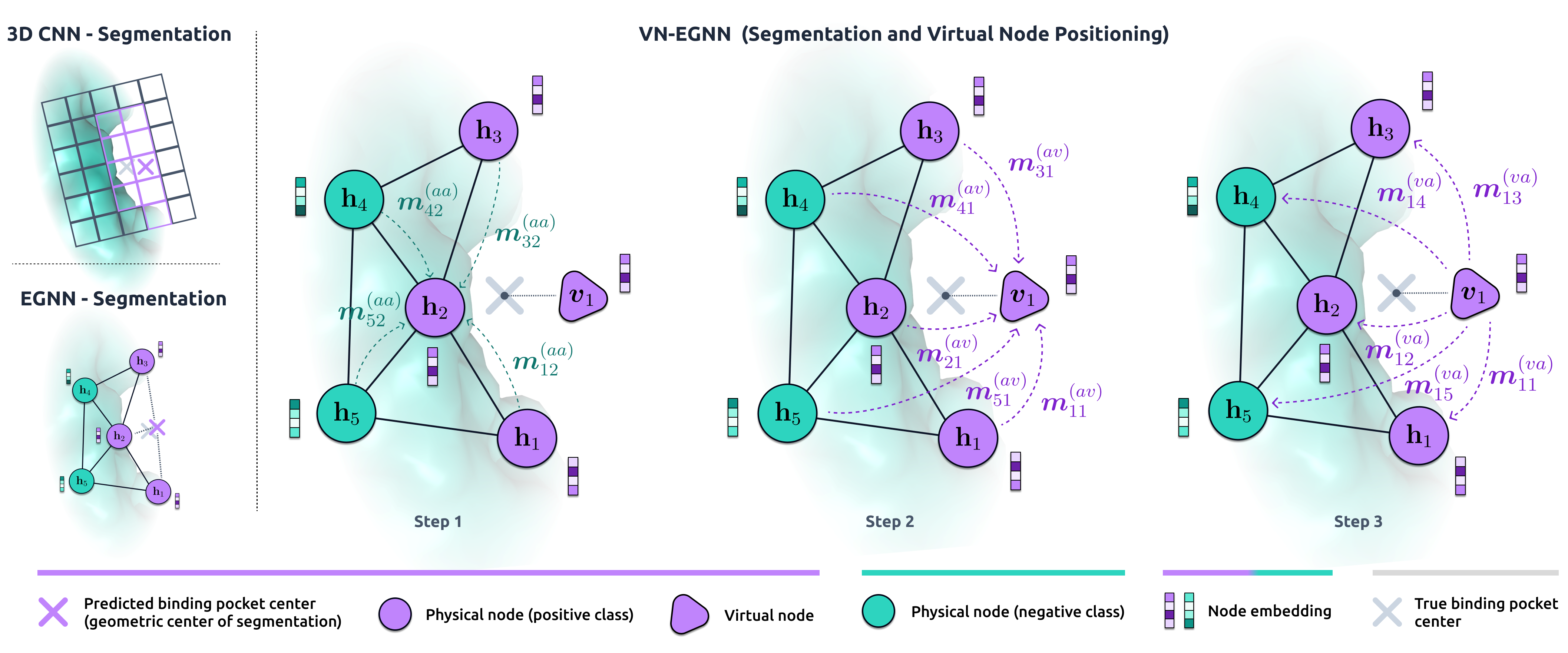
Figure 1: Overview of binding site identification methods. Top Left: Traditional methods, based on segmentation of a voxel grid, in which the pocket center is calculated as the geometric center of the positively labeled voxels. Bottom Left: Geometric Deep Learning approaches, such as EGNN, in which the pocket center is calculated as the geometric center of the positively labeled nodes. Right: VN-EGNN approach (ours): the predicted binding site center is the position of the virtual node after $L$ message passing layers.

Methods for Binding Site Identification. The identification of binding sites relies on the successful combination of physical, chemical and geometric information. Initially, machine learning methods for binding site prediction were based on carefully designed input features due to their tabular processing structure. For instance, FPocket (Le Guilloux et al., 2009) relies on Voronoi tessellation and alpha spheres (Liang et al., 1998) and additionally takes an electronegativity criterion into account. A random forest based method, which makes use of the protein surface, is P2Rank (Krivák & Hoksza, 2018). With the advent of end-to-end deep learning and especially with the breakthrough of convolutional (Lecun et al., 1998) and graph neural networks (GNNs) (Scarselli et al., 2009; Defferrard et al., 2016; Kipf & Welling, 2017; Gilmer et al., 2017; Satorras et al., 2021), the construction of input features can be learned which helped to advance predictive quality. For instance, DeepSite (Jiménez et al., 2017) is a voxel-based 3D convolutional neural network for binding site prediction. Convolutional operations on the 3D space are, however, computationally very demanding and so quickly other approaches to tackle binding site identification were developed, e.g., DeepSurf (Mylonas et al., 2021) or PointSite (Yan et al., 2022). DeepSurf operates on surface-based representations and places several voxelized grids on the protein’s surface, while PointSite is based on a form of sparse convolutions to reduce the computational overhead and keep sparse regions in the 3D space to be sparse. Typical convolutional networks, however, do not perform well at binding site identification, likely because of the irregularity of protein structures and due to the fact that proteins may be arbitrarily rotated and shifted in space (Zhang et al., 2023b). Thus, geometric deep learning approaches (Bronstein et al., 2021), most notably (graph-based) group equivariant architectures, such as EquiPocket (Zhang et al., 2023b), which are equivariant to the group of Euclidean transformations in the 3D space (E($3$)), should be powerful methods for binding site identification.

E($3$)-equivariant Graph Neural Networks. We use graph neural networks (GNNs) that are robust to transformations of the Euclidean group, i.e., rotations, reflections, and translations, as well as to permutations. From a technical point of view, equivariance of a function $f$ to certain transformations means that for any transformation parameter $g$ and all inputs $x$ we have $f(T_{g}(x))=S_{g}(f(x))\ ,$ where $T_{g}$ and $S_{g}$ denote transformations on the input and output domain of $f$, respectively (see App. C for further information). Equivariant operators applied to molecular graphs allow to preserve the geometric structure of the molecule. We build on E($n$)-equivariant GNNs (EGNNs) of Satorras et al. (2021) applied to the three dimensional space and the problem of binding site identification. In contrast to methods such as MACE (Batatia et al., 2022), Nequip (Batzner et al., 2022), PaiNN (Schütt et al., 2021) or SEGNN (Brandstetter et al., 2021), EGNNs operate on scalar features, e.g., distances, and use scale operations for coordinate updates. Thus, EGNNs operate efficiently (Villar et al., 2021) without resorting to compute-expensive higher order features, and, most importantly, allow for efficient coordinate update of virtual nodes.

Limitations of GNNs and a mitigation strategy. Graph neural networks can suffer from limited expressiveness (Morris et al., 2019; Xu et al., 2019), oversmoothing (Li et al., 2018; Rusch et al., 2023), or oversquashing (Alon & Yahav, 2021; Topping et al., 2022), which can lead to unfavourable learning dynamics or weak predictive performance. To improve the learning dynamics of GNNs, several works have introduced virtual nodes, sometimes called super-nodes or supersource-nodes, that are introduced into a message-passing scheme and connected to all other nodes. In a benchmark setting, Hu et al. (2020) showed that adding virtual nodes tends to increase the predictive performance. Hwang et al. (2022) provide a theoretical analysis of the benefits of virtual nodes in terms of expressiveness, demonstrate the increased expressiveness of GNNs with virtual nodes and also hint at the fact that such nodes can decrease oversmoothing. Alon & Yahav (2021) mention that virtual nodes might be used as a technique to overcome oversquashing effects. Cai et al. (2023) and Cai (2023) show that an MPNN with one virtual node, connected to all nodes, can approximate a Transformer layer. Low rank global attention (Puny et al., 2020) can be seen as one virtual node, which improves expressiveness. Practically, virtual nodes have already been suggested in the original work by Gilmer et al. (2017), and they were even mentioned earlier in Scarselli et al. (2009) and used in application areas such as drug discovery (Li et al., 2017; Pham et al., 2017; Ishiguro et al., 2019). Joshi et al. (2023) investigated the expressive power of EGNNs in greater detail and argue that these networks can suffer from oversquashing. In order to alleviate the oversquashing problem of EGNNs for binding site identification, we suggest to extend EGNNs with virtual nodes and introduce an adapted message passing scheme. We refer to this method as Virtual-Node Equivariant GNN (VN-EGNN). To the best of our knowledge, VN-EGNN is the first E($3$)-equivariant GNN architecture using virtual nodes (and thereby not relying on a priori knowledge).

EGNNs with virtual nodes for binding site identification. In accordance with previous approaches, we consider binding site identification as a segmentation task. While other methods are, e.g., based on voxel grids, our method is based on EGNNs with virtual nodes, where all atoms or residues of the protein (the physical entities) are represented by physical, i.e., a non-virtual, nodes in the graph (see Fig. 1, left). The objective is to correctly classify whether a node is within a certain radius of a region to which potential ligands can bind. Therefore, binding site identification can be considered as a node-level binary classification task and thus a semantic segmentation task. For this task, the ground truth is whether an atom was within a certain radius to experimentally observed protein binding ligands. In addition to node features, EGNNs act on coordinate features associated with each node, and both feature types are updated during message passing. While it appears straightforward to associate physical nodes with the protein’s atoms, it is a-priori unclear if the coordinate embeddings of virtual nodes are useful for the task at hand. In an initial experiment, we trained VN-EGNN to learn a semantic segmentation task using multiple virtual nodes to which we assigned random coordinates. In an analysis of the results, we could empirically observe that coordinates of the virtual nodes converged towards the actual physical binding positions of ligands on the protein (see App. F for further details and Fig. 1, right, for a visualization). The results of this initial experiment gave rise to the assumption that virtual nodes enable VN-EGNNs to form useful neural representations of binding sites and especially allow to predict locations of binding site centers. This, however, further implies that the binding site center itself may be a useful optimization target to train VN-EGNNs and, thus, we extended our objective to not only correctly predict whether physical nodes are close to binding regions, but also to directly take the distance between observed and predicted binding site centers into account. With this multi-modal objective, the coordinate embeddings of virtual nodes are trained to predict the locations of binding site centers. The remaining features of the virtual nodes are considered to form an abstract neural representation of a protein binding site.

Contributions. In this work, we aim at improving binding site identification through geometric deep learning methods. Here, we follow the approach of using EGNNs (Satorras et al., 2021; Zhang et al., 2023b) for identifying binding pockets. Although EGNNs are prime candidates for this task, they exhibit poor performance at binding site identification (Zhang et al., 2023b), which might be due to a) their lack of dedicated nodes that can learn representations of binding sites, and b) oversquashing effects which hamper learning (Alon & Yahav, 2021; Topping et al., 2022; Joshi et al., 2023). We aim at alleviating both problems by extending EGNNs with so-called virtual nodes. In this work, we contribute the following:
a) We propose a novel type of graph neural network geared towards the identification of binding sites of proteins.
b) We demonstrate that the virtual nodes in the message-passing scheme learn useful representations and accurate locations of binding pockets.
c) We assess the performance of other methods, baselines and our method on benchmarking datasets.

2 E($3$)-Equivariant Graph Neural Networks with Virtual Nodes

2.1 Notational Preliminaries

We give an overview on variable and symbol notation in App. A, and a more detailed description and discussion on how we represent proteins and binding sites in Sections B.1 and B.2 respectively. To quickly summarize, the coordinates of the $i$-th physical node, e.g., the location of an atom of a protein, are denoted as $\mathbf{x}_{i}\in\mathbb{R}^{3}$, and its other node features as $\bm{h}_{i}\in\mathbb{R}^{D}$. $l$ added as an index to symbols will indicate neural network layers, but might be omitted for simplicity sometimes if it is clear from the context. We will consider virtual nodes and the $k$-th virtual node coordinates will be denoted as $\bm{z}_{k}$, while the other virtual node features will be denoted as $\bm{v}_{k}$. We use upper-case bold letters to denote the matrices collecting the coordinates and features of the $N$ physical and the $K$ virtual nodes, respectively: $\bm{H}^{l}:=(\bm{h}_{1}^{l},\ldots,\bm{h}_{N}^{l})$, $\mathbf{X}^{l}:=(\mathbf{x}_{1}^{l},\ldots,\mathbf{x}_{N}^{l})$, $\bm{V}^{l}:=(\bm{v}^{l}_{1},\ldots,\bm{v}^{l}_{K})$, $\mathbf{Z}^{l}:=(\mathbf{z}^{l}_{1},\ldots,\mathbf{z}^{l}_{K})$.

We denote the graph, which VN-EGNN works upon as $\mathcal{G}$ and $\bm{A}$ as the associated adjacency matrix. $\mathcal{N}(i)$ indicates neighbouring nodes to node $i$ within $\mathcal{G}$ and edge features between nodes $i$ and $j$ as $a_{ij}$ (for two non-virtual nodes) and $d_{ij}$ (if $j$ is virtual). At training time, we might have access to node-level labels $y_{i}=1$ and $y_{i}=0$. We assume that in the training set we have access to a set of $M$ center coordinates $\{\mathbf{y}_{m}\}_{m=1}^{M}$ with $\mathbf{y}_{m}\in\mathbb{R}^{3}$, which the model should predict. We denote predicted node-level labels by $\hat{y}_{i}\in[0,1]$ and the set of $K$ predicted center coordinates from the model by $\{\hat{\mathbf{y}}_{k}\}_{k=1}^{K}$ with $\hat{\mathbf{y}}_{k}\in\mathbb{R}^{3}$.

2.2 EGNNs and their application to Binding Site Identification

EGNNs are straightforward to apply to proteins, when they are represented by a neighborhood graph $\mathcal{P}$, in which each node represents an atom and edges between two atoms represent spatially close atoms (distance between the atoms in the protein is below some threshold). To apply EGNNs, we first set $\mathcal{G}=\mathcal{P}$. For binding pocket identification, one could predict node labels $y_{i}$, which indicate whether the atom belongs to a binding pocket or not.

The physical nodes represent atoms and their initial coordinate features are set to the location of the atoms $\mathbf{x}^{0}_{i}$, and the initial node features $\bm{h}^{0}_{i}$ to, e.g., the atom or residue type. Then we apply the layer-wise message passing scheme $\left(\mathbf{X}^{l+1},\bm{H}^{l+1}\right)=\mathrm{EGNN}\left(\mathbf{X}^{l},\bm{H}^{l},\bm{A}\right)$ (Eqs. 1 to 4) as given by Satorras et al. (2021):

$$\bm{m}_{ij}=\bm{\phi}_{e}(\bm{h}_{i}^{l},\bm{h}_{j}^{l},\lVert\mathbf{x}_{i}^{l}-\mathbf{x}_{j}^{l}\rVert^{2},a_{ij})$$ (1)

$$\bm{m}_{i}=\sum_{j\in\mathcal{N}(i)}\bm{m}_{ij}$$ (2)

$$\mathbf{x}_{i}^{l+1}=\mathbf{x}_{i}^{l}+\frac{1}{|\mathcal{N}(i)|}\sum_{j\in\mathcal{N}(i)}\frac{\mathbf{x}_{i}^{l}-\mathbf{x}_{j}^{l}}{\lVert\mathbf{x}_{i}^{l}-\mathbf{x}_{j}^{l}\rVert}\phi_{x}(\bm{m}_{ij})$$ (3)

$$\bm{h}_{i}^{l+1}=\bm{\phi}_{h}\left(\bm{h}_{i}^{l},\bm{m}_{i}\right),$$ (4)

where $\bm{\phi}_{e}$, $\phi_{\mathbf{x}}$ and $\bm{\phi}_{h}$ denote multilayer-perceptrons (MLPs). To identify binding pockets, we can extract predictions $\hat{y}_{i}$ for each atom $i$ by a read-out function applied to the last message passing step $L$, i.e., we have: $\hat{y}_{i}=\sigma(\bm{w}^{\top}\bm{h}_{i}^{L})$ with an activation function $\sigma$ and parameters $\bm{w}$. Our model does not incorporate edge features, symbolized by $a_{ij}$. Hence, we will exclude these from the subsequent EGNN formulations and their related derivations.

2.3 VN-EGNN: Extension of EGNN with virtual nodes

We now extend $\mathcal{G}$ (which is set to the protein neighborhood graph $\mathcal{P}$ for the task of protein binding site identification) with a set of $K$ virtual nodes, which exhibit edges to all other nodes, which will allow us to learn representations of hidden geometric entities, such as binding sites, and simultaneously ameliorate oversquashing. To be able to process this extended graph, we modify EGNNs by locating the virtual nodes at coordinates $\mathbf{Z}=(\mathbf{z}_{1},\ldots,\mathbf{z}_{K})\in\mathbb{R}^{3}$ and associating them with a set of properties $\bm{V}=(\bm{v}_{1},\ldots,\bm{v}_{K})\in\mathbb{R}^{D}$. The new message passing scheme $\left(\mathbf{X}^{l+1},\bm{H}^{l+1},\mathbf{Z}^{l+1},\bm{V}^{l+1}\right)=\;\;\mathrm{VN\text{-}EGNN}\left(\mathbf{X}^{l},\bm{H}^{l},\mathbf{Z}^{l},\bm{V}^{l},\bm{A}\right)$ of a single VN-EGNN layer consists of three phases (Eqs. 7 to 10, Eqs. 11 to 14, and, Eqs. 15 to 18), in which the feature and coordinate embeddings of the physical nodes are updated twice:

$$\bm{h}^{l}_{i}\rightarrow\bm{h}^{l+\nicefrac{{1}}{{2}}}_{i}\rightarrow\bm{h}^{l+1}_{i},\quad\mathbf{x}^{l}_{i}\rightarrow\mathbf{x}^{l+\nicefrac{{1}}{{2}}}_{i}\rightarrow\mathbf{x}^{l+1}_{i}\quad\forall i$$ (5)

while virtual node embeddings are only updated once per message passing step

$$\bm{v}^{l}_{k}\rightarrow\bm{v}^{l+1}_{k},\quad\mathbf{z}^{l}_{k}\rightarrow\mathbf{z}^{l+1}_{k}\quad\forall k.$$ (6)

Message Passing Phase I between physical nodes (analogous to EGNN):

$$\bm{m}_{ij}^{(aa)}=\bm{\phi}_{e^{(aa)}}(\bm{h}_{i}^{l},\bm{h}_{j}^{l},\lVert\mathbf{x}_{i}^{l}-\mathbf{x}_{j}^{l}\rVert,a_{ij})$$ (7)

$$\bm{m}_{i}^{(aa)}=\frac{1}{|\mathcal{N}(i)|}\sum_{j\in\mathcal{N}(i)}\bm{m}_{ij}^{(aa)}$$ (8)

$$\mathbf{x}_{i}^{l+\nicefrac{{1}}{{2}}}=\mathbf{x}_{i}^{l}+\frac{1}{|\mathcal{N}(i)|}\sum_{j\in\mathcal{N}(i)}\frac{\mathbf{x}_{i}^{l}-\mathbf{x}_{j}^{l}}{\lVert\mathbf{x}_{i}^{l}-\mathbf{x}_{j}^{l}\rVert}\phi_{x^{aa}}(\bm{m}_{ij}^{(aa)})$$ (9)

$$\bm{h}_{i}^{l+\nicefrac{{1}}{{2}}}=\bm{h}_{i}^{l}+\bm{\phi}_{h^{(aa)}}\left(\bm{h}_{i}^{l},\bm{m}_{i}^{(aa)}\right).$$ (10)

Message Passing Phase II from physical nodes to virtual nodes:

$$\bm{m}_{ij}^{(av)}=\bm{\phi}_{e^{(av)}}(\bm{h}_{i}^{l+\nicefrac{{1}}{{2}}},\bm{v}_{j}^{l},\lVert\mathbf{x}_{i}^{l+\nicefrac{{1}}{{2}}}-\mathbf{z}_{j}^{l}\rVert,d_{ij})$$ (11)

$$\bm{m}_{j}^{(av)}=\frac{1}{N}\sum_{i=1}^{N}\bm{m}_{ij}^{(av)}$$ (12)

$$\mathbf{z}_{j}^{l+1}=\mathbf{z}_{j}^{l}+\frac{1}{N}\sum_{i=1}^{N}\frac{\mathbf{x}_{i}^{l+\nicefrac{{1}}{{2}}}-\mathbf{z}_{j}^{l}}{\lVert\mathbf{x}_{i}^{l+\nicefrac{{1}}{{2}}}-\mathbf{z}_{j}^{l}\rVert}\phi_{x^{av}}(\bm{m}_{ij}^{(av)})$$ (13)

$$\bm{v}_{j}^{l+1}=\bm{v}_{j}^{l}+\bm{\phi}_{h^{(av)}}\left(\bm{v}_{j}^{l},\bm{m}_{j}^{(av)}\right)$$ (14)

Message Passing Phase III from virtual node to physical nodes:

$$\bm{m}_{ij}^{(va)}=\bm{\phi}_{e^{(va)}}(\bm{v}_{i}^{l+1},\bm{h}_{j}^{l+\nicefrac{{1}}{{2}}},\lVert\mathbf{z}_{i}^{l+1}-\mathbf{x}_{j}^{l+\nicefrac{{1}}{{2}}}\rVert,d_{ji})$$ (15)

$$\bm{m}_{j}^{(va)}=\frac{1}{K}\sum_{i=1}^{K}\bm{m}_{ij}^{(va)}$$ (16)

$$\mathbf{x}_{j}^{l+1}=\mathbf{x}_{j}^{l+\nicefrac{{1}}{{2}}}+\frac{1}{K}\sum_{i=1}^{K}\frac{\mathbf{z}_{i}^{l+1}-\mathbf{x}_{j}^{l+\nicefrac{{1}}{{2}}}}{\lVert\mathbf{z}_{i}^{l+1}-\mathbf{x}_{j}^{l+\nicefrac{{1}}{{2}}}\rVert}\phi_{x^{va}}(\bm{m}_{ij}^{(va)})$$ (17)

$$\bm{h}_{j}^{l+1}=\bm{h}_{j}^{l+\nicefrac{{1}}{{2}}}+\bm{\phi}_{h^{(va)}}\left(\bm{h}_{j}^{l+\nicefrac{{1}}{{2}}},\bm{m}_{j}^{(va)}\right)$$ (18)

Here, $\bm{\phi}_{e^{(aa)}},\ldots,\bm{\phi}_{h^{(va)}}$ are again MLPs. The MLPs $\phi_{.}$ are layer-specific, i.e. $\phi^{l}_{.}$ and currently do not consider edge features $d_{ij}$ and $a_{ij}$. To keep the notation uncluttered, we skipped the layer index $l$ for the MLPs in the above formulae.

Initialization of virtual nodes in VN-EGNN. The $K$ virtual nodes are initially evenly distributed across a sphere using a Fibonacci grid (see Section E.4), of which the radius is defined as the distance between the protein center and its most distant atom. We initialize the virtual node properties $\bm{v}^{0}_{k}$ by averaging over the initial features $\bm{h}^{0}_{i}$.

2.4 Properties of VN-EGNN

The following proposition shows, that analogously to EGNNs, VN-EGNNs are equivariant with respect to roto-translations and reflections by construction.

Proposition 1.

E$(3)$-equivariant graph neural networks with virtual nodes as defined in Eqs. 7 to 18 are equivariant with respect to roto-translations and reflections of the input and virtual node coordinates.

Proof.

See App. D. ∎

Invariance with respect to the initial coordinates of the virtual nodes.

Note that Proposition 1 aims for equivariance with respect to rotations of the physical protein nodes $\mathbf{X}$ and arbitrary, but fixed initialized virtual nodes $\mathbf{Z}$ . We further want to have predictions, which are approximately invariant to differently chosen initial virtual node coordinates $\mathbf{Z}^{0}$. This ultimately leads to predictions that are approximately equivariant with respect to E($3$)-transformations of the physical protein nodes. In practice, we distribute the initial virtual node coordinates evenly on a sphere according to an algorithm, which constructs a spherical Fibonacci grid (Swinbank & James Purser, 2006). The algorithm provides spherically distributed grid points, which are fixed at certain locations in the 3D space. In order to achieve invariance with respect to differently chosen initial virtual node coordinates, we randomly rotate this grid of initial virtual node coordinates for each sample in every epoch, i.e. there is variation in the relative alignment of the Fibonacci grid points, that represent the virtual node positions, to physical protein nodes. Empirically, we observe that this training strategy leads to approximate invariance to different initializations of the virtual node coordinates (see Table G1).

A potential alternative strategy for initialization virtual node coordinates.

An idea to avoid random alignments between physical node coordinates and initial virtual node coordinates, would be, to change initial coordinates in an equivariant way with respect to E($3$) group transformations of the protein physical nodes. This could be achieved, e.g., by defining frames (Puny et al., 2022) based on Principal Component Analysis of physical protein node coordinates and by aligning the Fibonacci grid relative to these frames. Consequently, we would achieve that binding pocket predictions would change equivariantly with E($3$)- transformations of the protein. Thereby the definition of such frames via Principal Component Analysis (PCA) is possible up to certain degenerate cases, that occur with probability zero for proteins. Since the orientation of axes might still not be unique, a strategy might be to compute properties such as the overall molecular weight for each octant in the coordinate system spanned by PCA eigenvectors. The orientation can then be set, such that for the octant with the maximum overall molecular weight, all coordinates get positive values.

Virtual nodes ameliorate oversquashing by bounding the maximal shortest-path distance between nodes and required message-passing steps. Several works (Alon & Yahav, 2021; Topping et al., 2022; Di Giovanni et al., 2023) have investigated the relation between oversquashing and characteristics of the MPNN layers and the adjacency matrix. According to Topping et al. (2022) oversquashing is defined as $\frac{\partial h_{i}^{r+1}}{\partial h_{j}^{0}}$, which is the effect of that one node with index $i$ has on a node with index $j$ during learning, where the nodes are at a shortest-path distance of $r+1$. Critically, this quantity can be bounded by the model parameters of the involved MLPs and the topology of the graph (Di Giovanni et al., 2023), concretely the normalized adjacency matrix. We use Topping et al. (2022, Lemma 1), which states that $\left|\frac{\partial h_{i}^{r+1}}{\partial h_{j}^{0}}\right|\leq(\alpha\beta)^{r+1}(\hat{\bm{A}}^{r+1})_{ij}$ where $\alpha$ and $\beta$ are bounds on the element-wise gradients of the MLPs of the message-passing network, $h_{i}^{r+1}$ is one component of the node representation of node $i$ in message passing layer $r+1$. The quantity $r+1$ is both the number of message-passing layers and the shortest-path distance of nodes $i$ and $j$ in the graph, and $\hat{\bm{A}}$ is the normalized adjacency matrix, for which the diagonal values of the original matrix is set to $1$. The normalized adjacency matrix $\hat{\bm{A}}$ is a symmetric positive matrix that has a leading eigenvalue at $1$ (Perron, 1907; Frobenius, 1912), such all other the eigenvectors of all other eigenvalues of $\hat{\bm{A}}^{r}$ decay exponentially with $r$. Depending on the weights and activation functions of the MLPs, $|\alpha\beta|^{r+1}$ either grows or vanishes exponentially with $r$, which might lead to either exploding or vanishing gradients, respectively. Thus, learning can only be stabilized via keeping $r$ stable, which virtual nodes that are connected to all other nodes can provide since they bound both the maximal path distance and the necessary number of message-passing steps by $r+1=2$ .

Expressiveness of VN-EGNN.

The expressive power of GNNs is linked to their ability to distinguish non-isomorphic graphs. While a minimum of $k$ layers of an EGNN is required to distinguish two $k$-hop distinct graphs, one layer of VN-EGNN is presumed to be sufficient, as can be shown by the application of the Geometric Weisfeiler-Leman test, which serves as an upper bound on the expressiveness of EGNNs. Experimental findings on $k$-chain geometric graphs support this proposition and demonstrate the increased expressive power of VN-EGNN compared to EGNNs without virtual nodes. For further details and an empirical study see App. J.

2.5 Training VN-EGNNs

Objective. Previous methods, which consider binding site identification as a node-level prediction task (see Section 2.2) $\hat{y}_{n}=\sigma(\bm{w}^{\top}\bm{h}_{n}^{L})$, use a type of segmentation loss. The segmentation loss can be either the cross-entropy loss $\mathrm{CE}$:

$$\mathcal{L}_{\mathrm{segm}}=\frac{1}{N}\sum_{n=1}^{N}\mathrm{CE}(y_{n},\hat{y}_{n})$$

or the Dice loss, that is based on the continuous Dice coefficient (Shamir et al., 2019), with $\epsilon=1$:

$$\mathcal{L}_{\mathrm{dice}}\coloneqq 1-\frac{2\ \sum_{n=1}^{N}y_{n}\ \hat{y}_{n}+\epsilon}{\sum_{n=1}^{N}y_{n}+\sum_{n=1}^{N}\hat{y}_{n}+\epsilon}.$$

Our introduction of virtual nodes with coordinates allows to directly tackle the much more challenging problem to predict binding site region center points and to extract predictions for these points as outputs of the last EGNN layer. For each protein in the training set, we know the geometric center of the binding site, that we denote as $\{\mathbf{y}_{1},\ldots,\mathbf{y}_{M}\}$. The read-out $\hat{\mathbf{y}}_{k}$ for each virtual node $\hat{\mathbf{y}}_{k}:=\mathbf{z}_{k}^{L}$ ($1\leq i\leq K$) is just the coordinate embedding $\mathbf{z}_{k}^{L}$ in the last layer $L$. Each known binding site center should be detected by at least one virtual node, via its read-out, which leads to the following objective

$$\mathcal{L}_{\mathrm{bsc}}=\frac{1}{M}\sum_{m=1}^{M}\min_{k\in{1,\ldots,K}}\lVert\mathbf{y}_{m}-\hat{\mathbf{y}}_{k}\rVert^{2}.$$ (19)

The full objective of VN-EGNN for binding site identification is

$$\mathcal{L}=\mathcal{L}_{\mathrm{bsc}}+\mathcal{L}_{\mathrm{dice}},$$

in which the two terms could also be balanced against each other through a hyperparameter, which we found was not necessary though.

Self-Confidence Module. We employ a self-confidence module (Jumper et al., 2021; Zhang et al., 2023a), to assess the quality of predicted binding sites, by equipping each prediction with a confidence score. This allows a ranking of the predictions, similar to Krivák & Hoksza (2018). The confidence value, indicated by $\hat{c}_{k}$, is computed through $\hat{c}_{k}=\psi(\bm{v}_{k})$, with $\psi$ implemented as an MLP. During training, the target values for the confidence prediction are generated on-the-fly from the predicted positions $\hat{\mathbf{y}}_{i}$ and the closest known binding pocket center $\mathbf{y}_{m}$, in analogy with confidence scores for object detection methods in computer vision.

The confidence label for the $k$-th virtual node is obtained defined by (Zhang et al., 2023a):

$$c_{k}=\begin{cases}1-\frac{1}{2\gamma}\cdot\lVert\mathbf{y}_{k}-\hat{\mathbf{y}}_{k}\rVert&\text{if }\lVert\mathbf{y}_{k}-\hat{\mathbf{y}}_{k}\rVert\leq\gamma,\\ c_{0}&\text{otherwise}\end{cases},$$ (20)

with $c_{0}=0.001$, To align with the commonly accepted threshold value for the DCC/DCA success rates of 4Å we choose $\gamma=4$. The loss on the confidence score is squared loss:

$$\mathcal{L}_{\text{confidence}}=\frac{1}{K}\sum_{k=1}^{K}(c_{k}-\hat{c}_{k})^{2}.$$ (21)

Methods Param COACH420 HOLO4K^d PDBbind2020 (M) DCC$\uparrow$ DCA$\uparrow$ DCC$\uparrow$ DCA$\uparrow$ DCC$\uparrow$ DCA$\uparrow$ Fpocket (Le Guilloux et al., 2009)^b \ 0.228 0.444 0.192 0.457 0.253 0.371 P2Rank (Krivák & Hoksza, 2018)^c \ 0.464 0.728 0.474 0.787 0.653 0.826 DeepSite (Jiménez et al., 2017)^b 1.00 \ 0.564 \ 0.456 \ \ Kalasanty (Stepniewska-Dziubinska et al., 2020)^b 70.64 0.335 0.636 0.244 0.515 0.416 0.625 DeepSurf (Mylonas et al., 2021)^b 33.06 0.386 0.658 0.289 0.635 0.510 0.708 DeepPocket (Aggarwal et al., 2022b)^c \ 0.399 0.645 0.456 0.734 0.644 0.813 GAT (Veličković et al., 2018)^b 0.03 0.039(0.005) 0.130(0.009) 0.036(0.003) 0.110(0.010) 0.032(0.001) 0.088(0.011) GCN (Kipf & Welling, 2017)^b 0.06 0.049(0.001) 0.139(0.010) 0.044(0.003) 0.174(0.003) 0.018(0.001) 0.070(0.002) GAT + GCN^b 0.08 0.036(0.009) 0.131(0.021) 0.042(0.003) 0.152(0.020) 0.022(0.008) 0.074(0.007) GCN2 (Chen et al., 2020)^b 0.11 0.042(0.098) 0.131(0.017) 0.051(0.004) 0.163(0.008) 0.023(0.007) 0.089(0.013) SchNet (Schütt et al., 2017)^b 0.49 0.168(0.019) 0.444(0.020) 0.192(0.005) 0.501(0.004) 0.263(0.003) 0.457(0.004) EGNN (Satorras et al., 2021)^b 0.41 0.156(0.017) 0.361(0.020) 0.127(0.005) 0.406(0.004) 0.143(0.007) 0.302(0.006) EquiPocket (Zhang et al., 2023b)^b 1.70 0.423(0.014) 0.656(0.007) 0.337(0.006) 0.662(0.007) 0.545(0.010) 0.721(0.004) VN-EGNN (ours) 1.20 0.605(0.009) 0.750(0.008) 0.532(0.021) 0.659(0.026) 0.669(0.015) 0.820(0.010) a The standard deviation across training re-runs is indicated in parentheses. b Results from Zhang et al. (2023b). c Uses different training set and, thus, limited comparability. d This dataset represents a strong domain shift from the training data for all methods (except for P2Rank). Details on the domain shift in App. I.

Table 1: Performance at binding site identification in terms of DCC and DCA success rates.^a The first column provides the method, the second the number of parameters of the model, the fourth and the fifth column the performance on the COACH420 dataset, the sixth and seventh column the performance on the HOLO4K dataset, and the remaining columns the performance on PDBbind 2020. The best performing method(s) per column are marked bold. The second best in italics.

3 Experiments

3.1 Data

We use the benchmarking setting of Zhang et al. (2023b) performing experiments on four datasets for binding site identification: scPDB (Desaphy et al., 2015), PDBbind (Wang et al., 2004), COACH420 and HOLO4K. For details, see Section E.1.

Methods VN heterog. ESM COACH420 HOLO4K PDBbind2020 MP DCC$\uparrow$ DCA$\uparrow$ DCC$\uparrow$ DCA$\uparrow$ DCC$\uparrow$ DCA$\uparrow$ EGNN (Satorras et al., 2021)^b ✗ ✗ ✗ 0.156(0.017) 0.361(0.020) 0.127(0.005) 0.406(0.004) 0.143(0.007) 0.302(0.006) VN-EGNN (residue emb.) ✓ ✓ ✗ 0.503(0.022) 0.684(0.016) 0.438(0.019) 0.605(0.013) 0.551(0.017) 0.751(0.009) VN-EGNN (homog.) ✓ ✗ ✗ 0.497(0.014) 0.700(0.013) 0.414(0.023) 0.618(0.024) 0.502(0.029) 0.717(0.025) VN-EGNN (homog.) ✓ ✗ ✓ 0.575(0.008) 0.708(0.009) 0.479(0.012) 0.595(0.010) 0.649(0.010) 0.805(0.006) VN-EGNN (full) ✓ ✓ ✓ 0.605(0.009) 0.750(0.008) 0.532(0.021) 0.659(0.026) 0.669(0.015) 0.820(0.010) a The standard deviation across training re-runs is indicated in parentheses. b Results from Zhang et al. (2023b).

Table 2: Ablation study. The main components of the VN-EGNN architecture are ablated and tested for their performance on the benchmarking datasets. The first column reports the variant of the ablated method, the second column whether the method contains virtual nodes (VN), the third column whether the method applies heterogenous message-passing, and the fourth column whether ESM embeddings were used. The remaining columns are analogous to Table 1.

3.2 Evaluation

Methods compared. We compare the following binding site identification methods from different categories: Geometry-based: Fpocket (Le Guilloux et al., 2009) and P2Rank (Krivák & Hoksza, 2018). CNN-based: DeepSite (Jiménez et al., 2017), Kalasanty (Stepniewska-Dziubinska et al., 2020), DeepPocket (Aggarwal et al., 2022a) and DeepSurf (Mylonas et al., 2021). Topological graph-based: GAT (Veličković et al., 2018), GCN (Kipf & Welling, 2017), and GCN2 (Chen et al., 2020). Spatial graph-based: SchNet (Schütt et al., 2017), EGNN (Satorras et al., 2021), EquiPocket (Zhang et al., 2023b), and our proposed VN-EGNN.

Evaluation metrics. We used the DCC/DCA success rate, which are well-established metrics for binding site identification (see e.g., Chen et al., 2011). The DCC is defined as the distance between the predicted and known binding site centers, whereas the DCA is defined as the shortest distance between the predicted center and any atom of the ligand. Following Stepniewska-Dziubinska et al. (2020) and Zhang et al. (2023b), predictions within a certain threshold of DCC and DCA, are considered as successful, which is commonly referred to as DCC/DCA success rate. Adhering to these works, we maintained a threshold of 4Å throughout our experiments (for other thresholds, see Fig. 2). In line with Chen et al. (2011); Zhang et al. (2023b); Stepniewska-Dziubinska et al. (2020) for each protein only $M$ predicted binding sites with the highest self-confidence scores $\hat{c}_{k}$ are considered, where $M$ is the number of known binding sites of the protein. Subsequently, each predicted binding site was aligned with the closest real binding site and DCC/DCA success rate was calculated.

3.3 Implementation details.

We used AdamW (Loshchilov & Hutter, 2019) optimizer for 1500 epochs, selecting the best checkpoint based on the validation dataset. We used 5 VN-EGNN layers, where each layer consists of the three step message passing scheme described in Section 2.3, the feature and message size was set to 100, in all layers. Due to the possibility of different virtual nodes converging to identical locations, we employed Mean Shift Algorithm (Comaniciu & Meer, 2002), to cluster virtual nodes that are in close spatial proximity. By averaging their self-confidence scores and positions, we treated these clustered nodes as a single instance. Because of the large complexes in HOLO4K, we ran VN-EGNN for each chain and merged the predicted pocket centers. For the initial residue node features we used pre-trained ESM-2 (Lin et al., 2022) protein embeddings following Corso et al. (2023); Pei et al. (2023). For virtual nodes, we derived their features by averaging the residue node features across the entire protein. We used the position of the $\alpha$-carbons as residue node locations. Virtual nodes are connected to residue nodes solely, but not with each other. A linear layer was used to map these initial features to the required dimensions ($\bm{h}^{0}_{n}$, $\bm{v}_{k}^{0}$) of the model. Layer normalization and Dropout (Srivastava et al., 2014) was applied in each message passing layer. SiLU (Hendrycks & Gimpel, 2016) activation was used across all layers. Analogous to Pei et al. (2023) we applied normalization (divided by 5) and unnormalization (multiplied by 5) on the coordinates and used Huber loss (Huber, 1964) for the coordinates, which empirically proved to be slightly more effective. The learning rate was set to $10^{-3}$, after 100 epochs we reduced the learning rate by factor of $10^{-1}$ if the model did not improve for 10 epochs. For training we used 4x NVIDIA A100 40GB GPU with batch size set to 64 on each GPU. The training time was about 8 hours. Hyperparameters were selected based on a validation dataset where we spilt 10% of the training data (see Table E1).

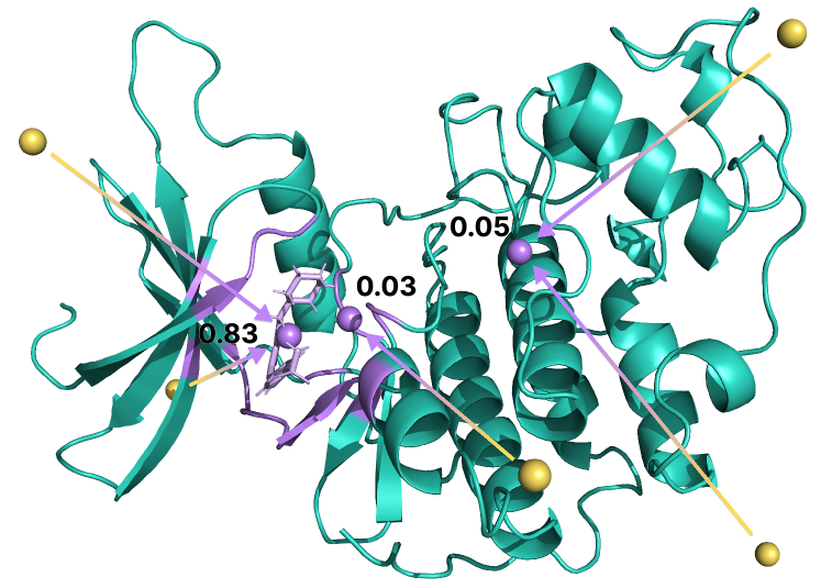
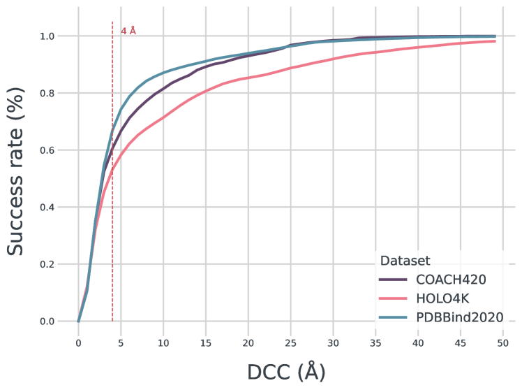
Figure 2: Left: Example of a prediction from our model: Initial positions of the virtual nodes are represented by the yellow spheres around the protein, the ground truth binding site is indicated by the light violet ligand, whereas violet regions on the protein represent the annotated binding site. The arrows indicate how the positions of the virtual nodes change from their initial positions. The violet spheres represent the clustered virtual node predictions with their associated self-confidence score. To simplify the visualization, not all initial positions of the virtual nodes are depicted in the figure. Right: DCC values for different thresholds. The x-axis denotes different thresholds for the distance of the predicted and known binding pocket center in Å. Distances below this threshold are considered as correctly found binding pockets. The y-axis denotes DCC success rate.

3.4 Results

Our experimental results demonstrate that our method VN-EGNN surpasses all prior approaches in terms of the DCC metric on COACH20, PDBbind2020 and even on the challenging HOLO4K dataset, see Table 1. On COACH20, VN-EGNN exhibits the best DCA score and on PDBbind it yields the same DCA score as P2Rank. Note that there is limited comparability with P2rank since this method uses a different training set that might be closer to HOLO4K. HOLO4K contains many complexes of symmetric proteins (see Section E.2), which should be considered as a strong domain shift to the training data and thus pose a problem for all methods except P2rank. For a more detailed discussion and a visual analysis we refer to App. I. Figure 2 shows an example of our model predictions.

3.5 Ablation study

Our proposed method comprises three main components as compared to typical other methods: (a) virtual nodes, (b) heterogenous message passing, and (c) pre-trained protein embeddings as node representations. We ablate these three components in a set of experiments (see Table 2). (a) Removing virtual nodes. We compared our model to a standard EGNN framework to determine the added value of virtual nodes. An EGNN architecture, was also used in Zhang et al. (2023b), but significantly extension. In this study we compared how a standard EGNN performs to our method. Table 2, shows that the standard EGNN architecture did not perform well. (b) Homogeneous message passing. Our approach to message passing, which is applied in a sequential manner, was contrasted with the traditional method where updates across nodes occur in parallel or homogeneously. This evaluation was further enriched by employing identical MLPs for both graph and virtual nodes across all layers, providing a direct comparison of the impact of our message passing strategy. (c) Atom type embeddings. We evaluated the impact of the type of embeddings, as outlined in Section 2.2. Table 2 illustrates that, regardless of the initial embeddings used, our model surpasses all preceding approaches in achieving higher DCC success rate across the COACH420 and PDBbind2020 datasets, except P2Rank. This was accomplished by adopting a one-hot encoding scheme solely for the amino acid types, complemented by an additional category for the virtual nodes.

4 Discussion and Conclusions.

Main findings. We have introduced a novel method that extends EGNNs (Satorras et al., 2021) with virtual nodes and a heterogeneous message-passing scheme. These new assets improve the learning dynamics by ameliorating the oversquashing problem and allow for learning representations of hidden geometric entities. Concretely, we have developed this method for binding site identification, for which our experiments show that VN-EGNN exhibits high predictive performance in terms of DCC and set a new state of the art on COACH420, HOLO4K and PDBbind2020. We attribute our improvement largely to the direct prediction of binding site centers, rather than inferring them from the geometric center of segmented areas, a common practice in earlier methods. Relying on segmentation can lead to inaccuracies, especially if a single erroneous prediction impacts the calculated center. Overall, VN-EGNN yields highly accurate predictions of binding site centers.

Comparison with previous work. We again emphasize that we are proposing a method for binding site identification and not docking, both of which are fundamental, but distinct, tasks in computational chemistry. VN-EGNN is an equivariant graph neural network approach, similar to Zhang et al. (2023b), however, with several differences. Contrary to the majority of preceding methodologies, which predominantly utilized some form of surface representation (Sanner et al., 1996; Eisenhaber et al., 1995), our approach deviated by solely relying on residue level information. By only using residue-level information, i.e. $\alpha$-carbons as physical nodes, our method is computationally much more efficient both during training and inference because the input graphs are smaller. These results on using only alpha-carbons underpins a finding by Jumper et al. (2021) that residue-level information implicitly contains all relevant side-chain conformations.

Implications. We expect that our empirical results and our new method re-new the interest in theoretically investigating the effect of virtual nodes on the expressivity and the oversquashing problem of GNNs. Practically, we envision that VN-EGNN will be a useful tool in molecular biology and structure-based drug design, which is regularly used to analyze proteins for potential binding pockets and their druggability. On the long run, this could make the drug development process more time- and cost-efficient.

Limitations. Our method is currently limited to predicting binding pockets of proteins similar to those in PDB. We expect that VN-EGNN can also be applied to other physical or geometric problems with hidden geometric entities, such as particle flows, however, their performance in these fields remains to be shown. Note that our method is not a docking method and thus cannot be used to dock ligands to protein structure. However, our predicted binding sites can be used as proposal regions for other methods, which could lead to improved performance and efficiency for docking methods.

Future work. We aim at using VN-EGNN to annotate all proteins in PDB with binding sites, and potentially a subset of the 200 million structures AlphaFold DB, with predicted binding pockets and release this annotated dataset.

Appendix:
VN-EGNN: E(3)-Equivariant Graph Neural Networks with Virtual Nodes Enhance Protein Binding Site Identification

This appendix is structured as follows:

• We provide an overview table of the notation in App. A.

• We then provide a more formal problem statement in App. B.

• For self-containedness, we give some background on group theory and equivariance in App. C.

• The proof of the equivariance of VN-EGNNs is given in App. D.

• Further details on the experimental settings are given in App. E.

• Details on the initial experiment can be found in App. F.

• An investigation of the approximate invariance with respect to initialization of the virtual node coordinates is proved in G.

• We included some visualizations in App. H.

• Statistics on the differences between the datasets and potential domain shifts and HOLO4K are provided in App. I.

• Finally, we included additional theory and experimental results on the expressivity of VN-EGNN in App. J.

Appendix A Notation Overview

Definition	Symbol/Notation	Type
number of physical nodes	$N$	$\mathbb{N}$
number of virtual nodes	$K$	$\mathbb{N}_{0}$
number of known binding pockets	$M$	$\mathbb{N}_{0}$
dimension of node features	$D$	$\mathbb{N}$
dimension of messages	$E$	$\mathbb{N}$
number of message passing layers/steps	$L$	$\mathbb{N}$
node indices	$i,j,k,n$	$\{1,...,K\}$ or $\{1,...,N\}$
binding pocket index	$m$	$\{1,...,M\}$
layer/step index	$l$	$\{1,...,L\}$
index set of 10 nearest neighbor atoms	$\mathcal{N}(i)$	$\{1,...,N\}^{10}$
physical node coordinates	$\mathbf{x}_{i}^{l}$	$\mathbb{R}^{3}$
virtual node coordinates	$\mathbf{z}_{j}^{l}$	$\mathbb{R}^{3}$
physical node feature representation	$\bm{h}_{i}^{l}$	$\mathbb{R}^{D}$
virtual node feature representation	$\bm{v}_{j}^{l}$	$\mathbb{R}^{D}$
edge feature between physical nodes	$a_{ij}$	$\mathbb{R}$
edge feature between physical and virtual node	$d_{ij}$	$\mathbb{R}$
matrix of all physical node coordinates	$\mathbf{X}$	$\mathbb{R}^{3\times N}$
matrix of all virtual node coordinates	$\mathbf{Z}$	$\mathbb{R}^{3\times K}$
matrix of all physical node feature representations	$\bm{H}$	$\mathbb{R}^{D\times N}$
matrix of all virtual node feature representations	$\bm{V}$	$\mathbb{R}^{D\times K}$
ground-truth node label	$y_{n}$	{0,1}
predicted node label	$\hat{y}_{n}$	$\left[0,1\right]$
ground-truth binding site center	$\mathbf{y}_{m}$	$\mathbb{R}^{3}$
prediction of binding site center	$\hat{\mathbf{y}}_{k}$	$\mathbb{R}^{3}$
messages*	$\bm{m}_{ij}^{(aa)}\!,\bm{m}_{ij}^{(av)}\!,\bm{m}_{ij}^{(va)}$	$\mathbb{R}^{E}$
neural networks for message passing*:
message calculation	$\bm{\phi}_{e^{(aa)}},\bm{\phi}_{e^{(av)}},\bm{\phi}_{e^{(va)}}$	$\mathbb{R}^{D}\!\times\!\mathbb{R}^{D}\!\times\!\mathbb{R}\!\times\!\mathbb{R}\rightarrow\mathbb{R}^{E}$
coordinate update	$\phi_{\mathbf{x}^{(aa)}},\phi_{\mathbf{x}^{(av)}},\phi_{\mathbf{x}^{(va)}}$ a	$\mathbb{R}^{E}\rightarrow\mathbb{R}$
feature update	$\bm{\phi}_{h^{(aa)}},\bm{\phi}_{h^{(av)}},\bm{\phi}_{h^{(va)}}$	$\mathbb{R}^{D}\!\times\!\mathbb{R}^{E}\rightarrow\mathbb{R}^{D}$
segmentation loss	$\mathcal{L}_{\mathrm{segm}}$	$\mathbb{R}^{N}\times\mathbb{R}^{N}\rightarrow\mathbb{R}$
binding site center loss	$\mathcal{L}_{\mathrm{bsc}}$	$\mathbb{R}^{3\times M}\times\mathbb{R}^{3\times K}\rightarrow\mathbb{R}$

• * The superscripts (aa), (av) and (va) represent the message passing direction (atom to atom, atom to virtual node, virtual node to
  atom).

Table A1: Overview of used symbols and notations

Appendix B Problem Statement

B.1 Representation of proteins.

The 3D structure of a protein is usually given by some measurement of its atoms that form the primary amino acid sequence of the protein and the absolute coordinates for the atoms are given as 3D points $\mathbf{x}\in\mathbb{R}^{3}$. The atoms themselves as well as the amino acids are characterized by their physical, chemical and biological properties. We assume that these properties are summarized by feature vectors $\bm{h}\in\mathbb{R}^{D}$, which are located at the atom centers (either of all the atoms or only the ones forming the protein backbone). We formally represent proteins by a neighborhood graph $\mathcal{P}=\left(\mathcal{P}_{N},\mathcal{P}_{E}\right)$ with $N$ atom-property pairs, i.e. $\mathcal{P}_{N}=\{(\mathbf{x}_{n},\bm{h}_{n})\}_{n=1}^{N}$ with $\mathbf{x}_{n}\in\mathbb{R}^{3}$ and $\bm{h}_{n}\in\mathbb{R}^{D}$ and a set of directed edges $\mathcal{P}_{E}$ which consist of atom-property pairs $\left(i,j\right)$. Each node $i$ has incoming edges from the 10 nearest nodes $j$ that are closer than 10Å according to the Euclidean distance $\lVert\mathbf{x}_{i}-\mathbf{x}_{j}\rVert$.

B.2 Representation of binding sites.

Binding sites are regions around or within proteins, to which ligands can potentially bind. Basically, one can either describe binding sites explicitly or implicitly. In their explicit representation binding sites would be directly described by the location specifics of the regions, where ligands are located, especially by a region center point. In their implicit representation, binding sites would be described by the atoms of the protein, which surround the ligand. Atoms close to the ligand would be marked as binding site atoms. It might be worth mentioning, that several binding sites per protein are possible.

Formally, for the explicit representation, we describe the (experimentally observed) binding site center points of $M$ distinct binding sites by $\mathbf{y}_{m}\in\mathbb{R}^{3}$ with $1\leq m\leq M$. For the implicit representation, we assign to each protein atom $n$ a label $y_{n}\in\{0,1\}$, which is set to $1$ if the atom center is within the threshold distance of observed binding ligands, and $0$ otherwise.

B.3 Objective.

From an abstract point of view, we want to learn a predictive machine learning model $\mathcal{F}$, parameterized by $\omega$, which maps proteins characterized by the positions of their atoms together with their properties to a binary prediction per atom, whether it might form a binding site and to $K$ 3D coordinates representing binding site region center points:

$$\text{\normalsize$\mathcal{F}_{\omega}$}:\bigtimes_{n=1}^{N}\left(\underbrace{\mathbb{R}^{3}\times\mathbb{R}^{D}}_{\begin{subarray}{c}\text{protein 3D atom}\\ \text{coords with}\\ \text{$D$-dim features}\end{subarray}}\right) \mapsto\underbrace{[0,1]^{N}}_{\begin{subarray}{c}\text{sem. segm.}\\ \text{protein atoms}\\ \\ \\ \text{ \normalsize$\coloneqq\mathcal{F}_{\omega}^{\mathrm{segm}}$}\end{subarray}}\times\underbrace{\bigtimes_{k=1}^{K}\mathbb{R}^{3}}_{\begin{subarray}{c}\text{pos. pred.}\\ \text{virt. nodes}\\ \\ \text{ \normalsize$\coloneqq\mathcal{F}_{\omega}^{\mathrm{bsc}}$}\end{subarray}}$$ (B.1)

$$\text{\normalsize$\mathcal{F}_{\omega}$}\left((\mathbf{x}_{1},\bm{h}_{1}),\ldots,(\mathbf{x}_{N},\bm{h}_{N})\right) =\left((\hat{y}_{1},\ldots,\hat{y}_{N}),(\hat{\mathbf{y}}_{1},\ldots,\hat{\mathbf{y}}_{K})\right)$$

$$\text{\normalsize$\mathcal{F}_{\omega}^{\mathrm{segm}}$}\left((\mathbf{x}_{1},\bm{h}_{1}),\ldots,(\mathbf{x}_{N},\bm{h}_{N})\right) \coloneqq\mathrm{proj}_{1}\text{\normalsize$\mathcal{F}_{\omega}$}\left((\mathbf{x}_{1},\bm{h}_{1}),\ldots,(\mathbf{x}_{N},\bm{h}_{N})\right)$$

$$\text{\normalsize$\mathcal{F}_{\omega}^{\mathrm{bsc}}$}\left((\mathbf{x}_{1},\bm{h}_{1}),\ldots,(\mathbf{x}_{N},\bm{h}_{N})\right) \coloneqq\mathrm{proj}_{2}\text{\normalsize$\mathcal{F}_{\omega}$}\left((\mathbf{x}_{1},\bm{h}_{1}),\ldots,(\mathbf{x}_{N},\bm{h}_{N})\right),$$

where $\mathrm{proj}_{i}$ is a projection, that gives the $i$-th component (i.e., prediction of the semantic segmenation part or coordinate predicitons or virtual nodes). Note, that for our predictive model, we use a fixed number $K$ of binding point centers, while indeed $M$ might have been observed for a specific protein.

B.4 Utilized Loss Functions.

Segmentation loss. For semantic segmentation (i.e., the prediction of $\mathcal{F}_{\omega}^{\text{segm}}$), we use a Dice loss, that is based on the continuous Dice coefficient (Shamir et al., 2019), with $\epsilon=1$:

$$\mathcal{L}_{\mathrm{dice}}=\mathrm{Dice}\left((y_{1},\ldots,y_{N}),(\hat{y}_{1},\ldots,\hat{y}_{N})\right)\coloneqq 1-\frac{2\ \sum_{n=1}^{N}y_{n}\ \hat{y}_{n}+\epsilon}{\sum_{n=1}^{N}y_{n}+\sum_{n=1}^{N}\hat{y}_{n}+\epsilon}$$ (B.2)

Perfect predictions lead to a Dice loss of $0$, while perfectly wrong predictions would lead to a Dice of $1$ (in case $\epsilon=0$ and the denominator is $>0$).

Binding site center loss. For prediction of the binding site region center points (i.e., the prediction of $\mathcal{F}_{\omega}^{\text{bsc}}$), we use the (squared) Euclidean distance between the set of predicted points and the set of observed ones. More specifically, we assume to be given $M$ observed center points $\{\mathbf{y}_{1},\ldots,\mathbf{y}_{M}\}$. Each of the binding site center points should be detected by at least one of the $K$ outputs from $\mathcal{F}_{\omega}^{\text{bsc}}$, which translates to using the minimum squared distance to any predicted center point for any of the observed center points:

$$\mathcal{L}_{\mathrm{bsc}}=\mathrm{Dist}\left(\{\mathbf{y}_{1},\ldots,\mathbf{y}_{M}\},\{\hat{\mathbf{y}}_{1},\ldots,\hat{\mathbf{y}}_{K}\}\right)\coloneqq\frac{1}{M}\sum_{m=1}^{M}\min_{k\in{1,\ldots,K}}\lVert\mathbf{y}_{m}-\hat{\mathbf{y}}_{k}\rVert^{2}.$$ (B.3)

Our optimization objective is then the sum of the $\mathrm{Dice}$ and the $\mathrm{Dist}$ loss:

$$\alpha\mathrm{Dice}\left((y_{1},\ldots,y_{N}),(\hat{y}_{1},\ldots,\hat{y}_{N})\right)+\mathrm{Dist}\left(\{\mathbf{y}_{1},\ldots,\mathbf{y}_{M}\},\{\hat{\mathbf{y}}_{1},\ldots,\hat{\mathbf{y}}_{K}\}\right)$$ (B.4)

with the hyperparameter $\alpha=1$.

Appendix C Background on Group Theory and Equivariance

A group in the mathematical sense is a set $G$ along with a binary operation $\circ:G\times G\rightarrow G$ with the following properties:

• Associativity: The group operation is associative, i.e. $(g\circ h)\circ k=g\circ(h\circ k)$ for all $g,h,k\in G$.

• Identity: There exists a unique identity element $e\in G$, such that $e\circ g=g\circ e=g$ for all $g\in G$.

• Inverse: For each $g\in G$ there is a unique inverse element $g^{-1}\in G$, such that $g\circ g^{-1}=g^{-1}\circ g=e$.

• Closure: For each $g,h\in G$ their combination $g\circ h$ is also an element of $G$.

A group action of group $G$ on a set $X$ is defined as a set of mappings $T_{g}:X\rightarrow X$ which associate each element $g\in G$ with a transformation on $X$, whereby the identity element $e\in G$ leaves $X$ unchanged ($T_{e}(x)=x\quad\forall x\in X$).

An example is the group of translations $\mathbb{T}$ on $\mathbb{R}^{n}$ with group action $T_{t}(x)=\mathbf{x}+\mathbf{t}\quad\forall\mathbf{x},\mathbf{t}\in\mathbb{R}^{n}$, which shifts points in $\mathbb{R}^{n}$ by a vector $\mathbf{t}$.

A function $f:X\rightarrow Y$ is equivariant to group $G$ with group action $T_{g}$ if there exists an equivalent group action $S_{g}:Y\rightarrow Y$ on $G$ such that

$$f(T_{g}(x))=S_{g}(f(x))\quad\forall x\in X,g\in G.$$

For example, a function $f:\mathbb{R}^{n}\rightarrow\mathbb{R}^{n}$ is translation-equivariant if a translation of an input vector $\mathbf{x}\in\mathbb{R}^{n}$ by $\mathbf{t}\in\mathbb{R}^{n}$ leads to the same transformation of the output vector $f(x)\in\mathbb{R}^{n}$, i.e. $f(\mathbf{x}+\mathbf{t})=f(\mathbf{x})+\mathbf{t}$.

Equivariant graph neural networks (EGNNs) $\psi$ as defined by Satorras et al. (2021) exhibit three types of equivariances:

1. Translation equivariance: EGNNs are equivariant to column-wise addition of a vector $\mathbf{t}\in\mathbb{R}^{n}$ to all points in a point cloud $\mathbf{X}\in\mathbb{R}^{n\times N}$: $\psi(\mathbf{X}+\mathbf{t})=\psi(\mathbf{X})+\mathbf{t}$.

2. Rotation and reflection equivariance: Rotation or reflection of all points in the point cloud by multiplication with an orthogonal matrix $\mathbf{R}\in\mathbb{R}^{n\times n}$ leads to an equivalent rotation of the output coordinates: $\psi(\mathbf{R}\mathbf{X})=\mathbf{R}\psi(\mathbf{X})$.

   The group spanning all translations, rotations and reflections in $\mathbb{R}^{n}$ is called Euclidean group, denoted E($n$), as it preserves Euclidean distances. A proof for E(n)-equivariance of VN-EGNN can be found in App. D.

3. Permutation equivariance: The numbering of elements in a point cloud or graph nodes does not influence the output, i.e. multiplication with a permutation matrix $\bm{P}\in\mathbb{R}^{N\times N}$ leads to the same permutation of output nodes: $\psi(\mathbf{X}\bm{P})=\psi(\mathbf{X})\bm{P}$. This property holds for message passing graph neural networks in general, as they aggregate and update node information based on local neighborhood structure, regardless of the order in which nodes are presented.

Appendix D Equivariance of VN-EGNN

In this section we show that the equivariance property of EGNN (Satorras et al., 2021) extends to VN-EGNN, i.e., that rotation and reflection by an orthogonal matrix $\mathbf{R}\in\mathbb{R}^{3\times 3}$, and translation by a vector $\mathbf{t}\in\mathbb{R}^{3}$ of atom and virtual node coordinates leads to an equivalent transformation of output coordinates while leaving node features invariant when applying the message passing steps of VN-EGNN.

Proposition 1.

(more formal) E($3$) equivariant graph neural networks with virtual nodes ($\mathrm{VN\text{-}EGNN}$) as defined by the message passing scheme $\left(\mathbf{X}^{l+1},\bm{H}^{l+1},\mathbf{Z}^{l+1},\bm{V}^{l+1}\right)=\mathrm{VN\text{-}EGNN}\left(\mathbf{X}^{l},\bm{H}^{l},\mathbf{Z}^{l},\bm{V}^{l},\bm{A}\right)$ in Eqs. 7 to 18 are equivariant with respect to reflections and roto-translations of the input and virtual node coordinates, i.e., the following holds (equivariance to reflections and roto-translations):

$$\left(\mathbf{R}\mathbf{X}^{l+1}+\mathbf{t},\bm{H}^{l+1},\mathbf{R}\mathbf{Z}^{l+1}+\mathbf{t},\bm{V}^{l+1}\right)=\mathrm{VN\text{-}EGNN}\left(\mathbf{R}\mathbf{X}^{l}+\mathbf{t},\bm{H}^{l},\mathbf{R}\mathbf{Z}^{l}+\mathbf{t},\bm{V}^{l}\right),$$ (D.1)

where the addition $\mathbf{X}^{l}+\mathbf{t}$ is defined as column-wise addition of the vector $\mathbf{t}$ to the matrix $\mathbf{X}$.

Proof.

We use the notation from Section 2.1 and proceed by tracking the propagation of node roto-translations through the VN-EGNN network. First, we want to show invariance in Eq. 7 in phase I of message passing, equivalently to Satorras et al. (2021), i.e.:

$$\bm{m}_{ij}^{(aa)}=\bm{\phi}_{e^{(aa)}}(\bm{h}_{i}^{l},\bm{h}_{j}^{l},\lVert\mathbf{R}\mathbf{x}_{i}^{l}+\mathbf{t}-[\mathbf{R}\mathbf{x}_{j}^{l}+\mathbf{t}]\rVert^{2},a_{ij})=\bm{\phi}_{e^{(aa)}}(\bm{h}_{i}^{l},\bm{h}_{j}^{l},\lVert\mathbf{x}_{i}^{l}-\mathbf{x}_{j}^{l}\rVert^{2},a_{ij})$$ (D.2)

Assuming the initial node features $\bm{h}^{0}_{i}$ and edge representations $a_{ij}$ do not encode information about the original coordinates $\mathbf{x}^{0}_{i}$, it remains to be shown that the Euclidean distance between two nodes is also invariant to translation and rotation:

$$\begin{split}\lVert\mathbf{R}\mathbf{x}_{i}^{l}+\mathbf{t}-[\mathbf{R}\mathbf{x}_{j}^{l}+\mathbf{t}]\rVert^{2}&=\lVert\mathbf{R}\mathbf{x}_{i}^{l}-\mathbf{R}\mathbf{x}_{j}^{l}\rVert^{2}\\ &=(\mathbf{x}_{i}^{l}-\mathbf{x}_{j}^{l})^{\top}\mathbf{R}^{\top}\mathbf{R}(\mathbf{x}_{i}^{l}-\mathbf{x}_{j}^{l})\\ &=(\mathbf{x}_{i}^{l}-\mathbf{x}_{j}^{l})^{\top}\mathbf{I}(\mathbf{x}_{i}^{l}-\mathbf{x}_{j}^{l})\\ &=\lVert\mathbf{x}_{i}^{l}-\mathbf{x}_{j}^{l}\rVert^{2}\end{split}$$ (D.3)

Consequently, the sum over messages (Eq. 8) and the feature update function (Eq. 10), which only uses the summed messages and previous node features as input, are invariant as well, leaving the intermediate output feature representations $\bm{h}^{l+\nicefrac{{1}}{{2}}}_{i}$ independent of coordinate transformations.

For the remaining equation (Eq. 9) of phase I the equivariance property can be shown as follows, where Eq. D.3 is used in the first equality:

$$\begin{split}\mathbf{R}\mathbf{x}_{i}^{l}+\mathbf{t}+\frac{1}{\mathcal{N}(i)}\sum_{j\in\mathcal{N}(i)}&\frac{\mathbf{R}\mathbf{x}_{i}^{l}+\mathbf{t}-[\mathbf{R}\mathbf{x}_{j}^{l}+\mathbf{t}]}{\lVert\mathbf{R}\mathbf{x}_{i}^{l}+\mathbf{t}-[\mathbf{R}\mathbf{x}_{j}^{l}+\mathbf{t}]\rVert}\phi_{x^{aa}}(\bm{m}_{ij}^{(aa)})\\ &=\mathbf{R}\mathbf{x}_{i}^{l}+\mathbf{t}+\frac{1}{\mathcal{N}(i)}\sum_{j\in\mathcal{N}(i)}\frac{\mathbf{R}\mathbf{x}_{i}^{l}+\mathbf{t}-[\mathbf{R}\mathbf{x}_{j}^{l}+\mathbf{t}]}{\lVert\mathbf{x}_{i}^{l}-\mathbf{x}_{j}^{l}\rVert}\phi_{x^{aa}}(\bm{m}_{ij}^{(aa)})\\ &=\mathbf{R}\mathbf{x}_{i}^{l}+\mathbf{t}+\frac{1}{|\mathcal{N}(i)|}\;\;\mathbf{R}\!\!\sum_{j\in\mathcal{N}(i),j\neq i}\frac{\mathbf{x}_{i}^{l}-\mathbf{x}_{j}^{l}}{\lVert\mathbf{x}_{i}^{l}-\mathbf{x}_{j}^{l}\rVert}\phi_{x^{aa}}(\bm{m}_{ij}^{(aa)})\\ &=\mathbf{R}\left(\mathbf{x}_{i}^{l}+\frac{1}{|\mathcal{N}(i)|}\sum_{j\in\mathcal{N}(i),j\neq i}\frac{\mathbf{x}_{i}^{l}-\mathbf{x}_{j}^{l}}{\lVert\mathbf{x}_{i}^{l}-\mathbf{x}_{j}^{l}\rVert}\phi_{x^{aa}}(\bm{m}_{ij}^{(aa)})\right)+\mathbf{t}\\ &=\mathbf{R}\mathbf{x}_{i}^{l+\nicefrac{{1}}{{2}}}+\mathbf{t}\end{split}$$ (D.4)

In phase II of message passing, we input the updated physical node coordinates $\mathbf{R}\mathbf{x}_{i}^{l+\nicefrac{{1}}{{2}}}+\mathbf{t}$ from Eq. D.4 together with virtual node coordinates $\mathbf{R}\mathbf{z}_{j}^{l}+\mathbf{t}$, both subjected to identical rotation and translation. Invariance of Eqs. 11, 12 and 14 can be deduced similarly to above, using the invariance properties of node features $\bm{h}^{l+\nicefrac{{1}}{{2}}}_{i}$ and $\bm{v}^{l}_{i}$, edge features $a_{ij}$ and $d_{ij}$, and Euclidean distance (Eq. D.3):

$$\begin{split}\bm{m}_{ij}^{(av)}&=\bm{\phi}_{e^{(av)}}(\bm{h}_{i}^{l+\nicefrac{{1}}{{2}}},\bm{v}_{j}^{l},\lVert\mathbf{R}\mathbf{x}_{i}^{l+\nicefrac{{1}}{{2}}}+\mathbf{t}-[\mathbf{R}\mathbf{z}_{j}^{l}+\mathbf{t}]\rVert^{2},d_{ij})\\ &=\bm{\phi}_{e^{(av)}}(\bm{h}_{i}^{l+\nicefrac{{1}}{{2}}},\bm{v}_{j}^{l},\lVert\mathbf{x}_{i}^{l+\nicefrac{{1}}{{2}}}-\mathbf{z}_{j}^{l}\rVert^{2},d_{ij})\end{split}$$ (D.5)

Thus, the output virtual node features $\bm{v}_{j}^{l+1}$ are invariant to roto-translations of node coordinates. Note that reflections are also covered by Eq. D.4 since the distance of two points does not change under reflection.

Equivariance of output virtual node coordinates $\mathbf{z}_{j}^{l+1}$ follows analogously to Eq. D.4:

$$\mathbf{R}\mathbf{z}_{j}^{l}+\mathbf{t}+\frac{1}{N}\sum_{i=1}^{N}\frac{\mathbf{R}\mathbf{x}_{i}^{l+\nicefrac{{1}}{{2}}}+\mathbf{t}-[\mathbf{R}\mathbf{z}_{j}^{l}+\mathbf{t}]}{\lVert\mathbf{R}\mathbf{x}_{i}^{l+\nicefrac{{1}}{{2}}}+\mathbf{t}-[\mathbf{R}\mathbf{z}_{j}^{l}+\mathbf{t}]\rVert}\phi_{x^{av}}(\bm{m}_{ij}^{(av)})=\mathbf{R}\mathbf{z}_{j}^{l+1}+\mathbf{t}$$ (D.6)

The same derivations of message invariance

$$\begin{split}\bm{m}_{ij}^{(va)}&=\bm{\phi}_{e^{(va)}}(\bm{v}_{i}^{l+1},\bm{h}_{j}^{l+\nicefrac{{1}}{{2}}},\lVert R\mathbf{z}_{i}^{l+1}+\mathbf{t}-[\mathbf{R}\mathbf{x}_{j}^{l+\nicefrac{{1}}{{2}}}+\mathbf{t}]\rVert^{2},d_{ji})\\ &=\bm{\phi}_{e^{(va)}}(\bm{v}_{i}^{l+1},\bm{h}_{j}^{l+\nicefrac{{1}}{{2}}},\lVert\mathbf{z}_{i}^{l+1}-\mathbf{x}_{j}^{l+\nicefrac{{1}}{{2}}}\rVert^{2},d_{ji})\end{split}$$ (D.7)

and coordinate equivariance

$$\mathbf{R}\mathbf{x}_{j}^{l+\nicefrac{{1}}{{2}}}+\mathbf{t}+\frac{1}{K}\sum_{i=1}^{K}\frac{\mathbf{R}\mathbf{z}_{i}^{l+1}+\mathbf{t}-[\mathbf{R}\mathbf{x}_{j}^{l+\nicefrac{{1}}{{2}}}+\mathbf{t}]}{\lVert\mathbf{R}\mathbf{z}_{i}^{l+1}+\mathbf{t}-[\mathbf{R}\mathbf{x}_{j}^{l+\nicefrac{{1}}{{2}}}+\mathbf{t}]\rVert}\phi_{x^{va}}(\bm{m}_{ij}^{(va)})=\mathbf{R}\mathbf{x}_{j}^{l+1}+\mathbf{t}$$ (D.8)

can be applied to phase III (Eqs. 15 to 18), proving that invariance of feature representations $\bm{h}_{j}^{l+1}$ and equivariance of coordinates $\mathbf{x}_{j}^{l+1}$ holds true for physical nodes as well, thus, proving Proposition 1.

∎

Appendix E Experimental Settings

E.1 Datasets

scPDB (Desaphy et al., 2015) is a frequently utilized dataset for binding site prediction (Kandel et al., 2021; Stepniewska-Dziubinska et al., 2020), encompassing both protein and ligand structures. We employed the 2017 release of scPDB in the training and validation. This release comprises 17,594 structures, 16,034 entries, 4,782 proteins, and 6,326 ligands. Structures were clustered based on their Uniprot IDs. From each cluster, protein structures with the longest sequences were selected, in alignment to the strategies used in Kandel et al. (2021) and Zhang et al. (2023b).

(Source: https://github.com/jivankandel/PUResNet/blob/main/scpdb_subset.zip)

PDBbind (Wang et al., 2004) is a widely recognized dataset integral to the study of protein-ligand interactions. This dataset provides detailed 3D structural information of proteins, ligands, and their respective binding sites, complemented by rigorously determined binding affinity values derived from laboratory evaluations. For our work, we draw upon the v2020 edition, which is divided into two sets: the general set (comprising 14,127 complexes) and the refined set (containing 5,316 complexes). While the general set encompasses all protein-ligand interactions, only the refined set, curated for its superior quality from the general collection, is used in our experiments.

(Source: http://www.pdbbind.org.cn/download/PDBbind_v2020_refined.tar.gz)

COACH420 and HOLO4K are benchmark datasets utilized for the prediction of binding sites, as originally detailed by Krivák & Hoksza (2018). Following the methodologies of Krivák & Hoksza (2018); Mylonas et al. (2021); Aggarwal et al. (2022a), we adopt the so-called mlig subsets from each of these datasets, which encompass the significant ligands pertinent to binding site prediction. Note that the HOLO4K contains many multi-chain systems and complexes with multiple copies of the protein (see Section App. I), such that this dataset’s distribution is strongly differs from the other datasets.

(Source: https://github.com/rdk/p2rank-datasets)

For comprehensive data preparation across all datasets, solvent atoms were excluded and erroneous structures were removed.

E.2 Hyperparameters and hyperparameter selection

Table E1 shows the evaluated hyperparameters. Bold indicates the parameters used in final model.

hyperparmater	considered and selected values
optimizer	{AdamW, Adam }
learning rate	$\{\mathbf{0.001},0.0001\}$
activation function	{ SiLU, ReLU }
dimension of node features $D$	$\{20,30,\textbf{100}\}$
dimension of the messages $P$	$\{40,50,\textbf{100}\}$
number of message passing layers/steps $L$	$\{2,3,4,\textbf{5}\}$
number of virtual nodes $K$	$\{4,\textbf{8}\}$
Huber loss $\delta$	$\{1\}$

Table E1: A list of considered and selected hyperparameters.

E.3 Inference Time Evaluation

Our model’s prediction time depends on the protein size. We demonstrate this by reporting inference times for two proteins:

• 3LPK protein (910 residues), 2.367 seconds

• 1ODI protein (1,410 residues), 3.809 seconds

E.4 Fibonacci grid

The Fibonacci grid (Swinbank & James Purser, 2006) offers a solution for evenly distributing points on a sphere. We chose this method to obtain the starting coordinates of virtual nodes for its simplicity and efficiency. To prevent virtual nodes from starting at identical locations in subsequent iterations, we apply random rotation of the sphere for each sample in every epoch.

Appendix F Initial experiment

Fig. F1 shows the training curves for a VN-EGNN during the development phase. VN-EGNN were only trained to minimize the segmentation loss $\mathcal{L}_{\mathrm{segm}}$. Even in the absence of a the binding site center loss $\mathcal{L}_{\mathrm{bsc}}$, the virtual nodes tend to converge towards the actual binding site center. This finding inspired us to further refine the position of the virtual nodes by including it directly to the optimization objective, which further improved the results significantly.

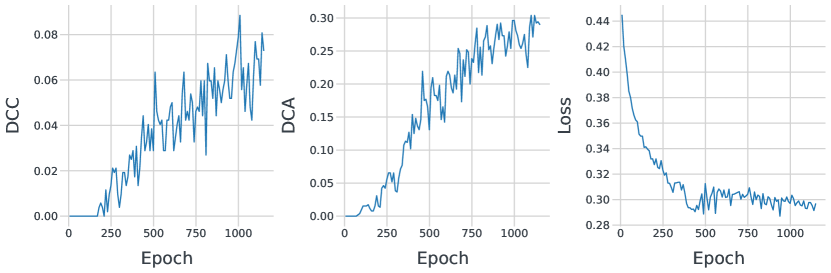
Figure F1: Validation curves of a VN-EGNN during development. Despite only being trained to minimize the segmentation loss, the virtual nodes converged towards the known binding sites. Left: DCC success rate during training. Middle: DCA success rate during training. Right: Segmentation loss during training.

Appendix G Invariance and initial coordinates of virtual nodes.

As stated in Section 2.4, we randomly rotate the grid of initial virtual nodes for each sample during training in order to achieve approximate invariance with respect to the initial coordinates of the virtual nodes. In an additional experiment, we evaluate how different relative positions of the virtual nodes to the protein affect the method performance. To investigate this, we randomly rotate the protein within the Fibonacci grid and perform inference on the proteins of the benchmarking datasets. The results of this experiment are presented in Table G1. Overall, the results show that there is hardly any change of the DCC and DCA metric across different random rotations. Therefore we conclude that our method VN-EGNN achieves approximate invariance to the initial coordinates of the virtual nodes via data augmentation during training.

Dataset	DCC	DCA
COACH420	0.612(0.005)	0.741(0.006)
HOLO4Kd	0.524(0.002)	0.632(0.002)
PDBbind2020	0.702(0.001)	0.833(0.002)

Table G1: Mean Performance at binding site identification in terms of DCC and DCA success rates together with their standard deviations (in parentheses). Means and standard deviations are across different random rotations of the Fibonacci grid.

Appendix H Visualizations

Fig. H.1 shows exemplary model predictions visualized with Pymol.

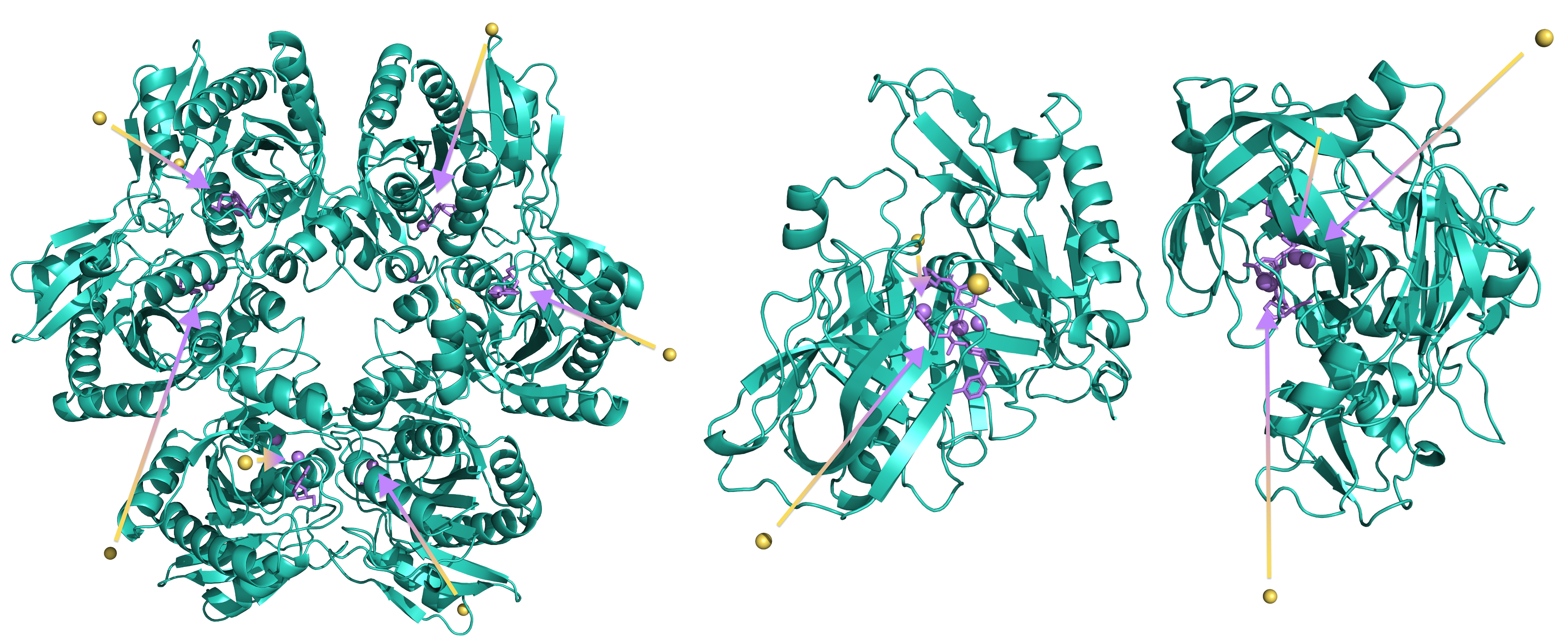
Figure H.1: Examples of Detected Binding Sites: Visualization and Analysis. We visualized two distinct proteins using Pymol, where the initial positions of the virtual nodes are represented by yellow spheres, were the violet spheres indicate the virtual nodes following $L$ message passing steps. The violet molecules indicate the position of the ligand as in the original PDB file. The arrows indicate the starting positions and the predicted positions of the virtual nodes. The visualization demonstrates that our model distributes the virtual nodes amongst various possible binding positions. The visualizations show the predicted positions after applying clustering as described in Section 1. To simplify the visualization, not all initial positions of the virtual nodes are depicted in the figure. Left:1odi Right: 3lpk.

Further, we visualize the learned virtual node features, grouped by the corresponding protein’s target classification according to the ChEMBL (Gaulton et al., 2011) database to analyze whether these representations contain relevant information about the protein/binding pocket (Fig. H.2).

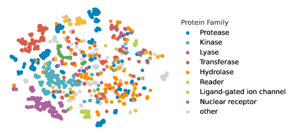
Figure H.2: T-SNE embeddings of virtual node features of the best ranked pockets for each protein in the PDBbind2020 dataset colored by protein family according to ChEMBL. The eight largest protein classes are shown, remaining proteins are colored in grey.

Appendix I Domain shift of the HOLO4K dataset

The HOLO4K benchmark comprises a large set of protein complexes and their annotated binding sites. HOLO4K has often been used as a benchmarking dataset (Krivák & Hoksza, 2018), while it exhibits different characteristics than other datasets, such as scPDB, COACH420 and PDBBind2020. The number of chains per sample, i.e. PDB file, is larger than in these datasets (see  Fig. I.1), and also the number of binding sites per entry is higher (see  Fig. I.1). HOLO4K contains many symmetric units of large complexes which lead to these statistics. Thus, for machine learning methods trained on scPDB, the HOLO4K dataset represents a difficult test case due to the mentioned domain shifts.

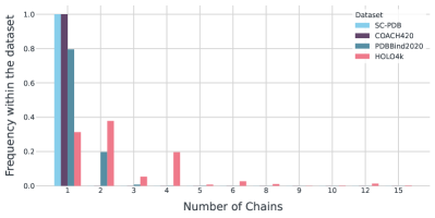
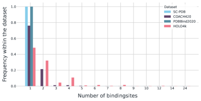
Figure I.1: Histogram of the number of protein chains (left) and of the number of binding sites frequency (right) per sample for each of the datasets used in this study. Note that the HOLO4K dataset has highly different characteristics compared to the other datasets and thus represents a strong domain shift for methods trained on scPDB.

Appendix J Expressiveness of VN-EGNN

The expressive power of GNNs is often described in terms of their ability to distinguish non-isomorphic graphs. The Weisfeiler-Leman (WL) (Weisfeiler & Leman, 1968) test, an iterative method to determine whether two attributed graphs are isomorphic, provides an upper bound to the expressiveness of GNNs. To extend the applicability of this framework to geometric graphs, Joshi et al. (2023) introduced the Geometric Weisfeiler-Leman test (GWL) which assesses whether two graphs are geometrically isomorphic.

Definitions (Joshi et al., 2023): Two graphs $\mathcal{G}_{1}$ and $\mathcal{G}_{2}$ with node features $h_{i}^{\mathcal{G}_{j}}$ and coordinates $\mathbf{x}_{i}^{\mathcal{G}_{j}}$ for $j\in\{1,2\}$ are called geometrically isomorphic if there exists an edge-preserving bijection $b:\mathcal{V}(\mathcal{G}_{1})\rightarrow\mathcal{V}(\mathcal{G}_{2})$ between their corresponding node indices $\mathcal{V}(\mathcal{G}_{j})$, such that their geometric features are equivalent up to $E(n)$ group actions, i.e. global rotations/reflections $\bm{R}$ and translations $\mathbf{t}$:

$$\left(h_{b(i)}^{\mathcal{G}_{2}},\mathbf{x}_{b(i)}^{\mathcal{G}_{2}}\right)=\left(h_{i}^{\mathcal{G}_{1}},\bm{R}\mathbf{x}_{i}^{\mathcal{G}_{1}}+\mathbf{t}\right)\quad\forall i\in\mathcal{V}(\mathcal{G}_{1}).$$ (J.1)

Two graphs $\mathcal{G}_{1}$ and $\mathcal{G}_{2}$ are called $k$-hop distinct if for all graph isomorphisms $b$, there is some node $i\in\mathcal{V}(\mathcal{G}_{1}),b(i)\in\mathcal{V}(\mathcal{G}_{2})$ such that the corresponding $k$-hop neighborhood subgraphs $\mathcal{N}_{i}^{(\mathcal{G}_{1},k)}$ and $\mathcal{N}_{b(i)}^{(\mathcal{G}_{2},k)}$ are distinct. Otherwise, if $\mathcal{N}_{i}^{(\mathcal{G}_{1},k)}$ and $\mathcal{N}_{b(i)}^{(\mathcal{G}_{2},k)}$ are identical up to group actions for all $i\in\mathcal{V}(\mathcal{G}_{1})$, we say $\mathcal{G}_{1}$ and $\mathcal{G}_{2}$ are $k$-hop identical.

In addition to iteratively updating node colors depending on node features in the local neighborhood analogously to the WL test, GWL keeps track of $E(n)$-equivariant hash values of each node’s local geometry, i.e., distances to and angles between neighboring nodes. Thus, $k$ iterations of GWL are necessary and sufficient to distinguish any $k$-hop distinct, $(k-1)$-hop identical geometric graphs (Joshi et al., 2023).

Proposition 2.

Any two geometrically distinct graphs $\mathcal{G}_{1}$ and $\mathcal{G}_{2}$, where the underlying attributed graphs are isomorphic, can be distinguished with one iteration of GWL by adding one virtual node connected to all other nodes.

Proof.

For $1$-hop distinct graphs one iteration of GWL suffices to distinguish them even without virtual nodes and, thus, the proposition holds.

Now, we assume that $\mathcal{G}_{1}$ and $\mathcal{G}_{2}$ are $k$-hop distinct and $(k-1)$-hop identical for any $k>1\in\mathbb{N}$ and place one virtual node connected to all other nodes in an equivalent position in both graphs.

Note that finding equivalent virtual node positions is not trivial, as there is no straight-forward way to spatially align the two graphs. However, for any $(k-1)$-hop sub-graph in $\mathcal{G}_{1}$ there exists an identical sub-graph in $\mathcal{G}_{2}$, such that the neighborhood structure between matching sub-graphs is preserved. We align the two graphs in space by overlaying one such pair of $(k-1)$-hop sub-graphs (consisting of more than two nodes that are not arranged in a straight line) and position the virtual node in the same coordinates in both aligned graphs.

Since the virtual node is connected to each node in the graph, its $1$-hop neighborhood and therefore the receptive field of the first GWL iteration contains the entire graph. Due to the $k$-hop distinctness of the graphs, there exists at least one node for which the geometric orientation relative to the matched subgraph deviates between $\mathcal{G}_{1}$ and $\mathcal{G}_{2}$. Thus, the hash values corresponding to the virtual nodes’ geometric information differ, and the graphs can be distinguished by only one iteration of GWL. ∎

As $k$ iterations of GWL act as an upper bound on the expressiveness of a $k$-layer geometric GNN, we propose that one layer of VN-EGNN is sufficient to distinguish two $k$-hop distinct graphs while without virtual nodes $k$ EGNN layers are necessary to complete the same task.

We demonstrate this on the example of $n$-chain geometric graphs, where each pair of graphs comprises $n$ nodes arranged in a line and two end points with distinct orientations (Fig. J.1). These graphs are ($\lfloor{\frac{n}{2}}\rfloor+1$)-hop distinct and should therefore be distinguishable by ($\lfloor{\frac{n}{2}}\rfloor+1$) EGNN layers or ($\lfloor{\frac{n}{2}}\rfloor+1$) iterations of GWL.

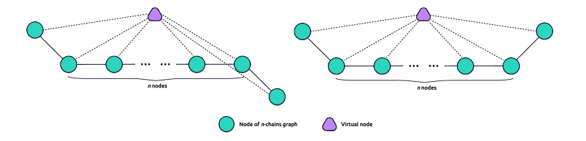
Figure J.1: A pair of $n$-chain geometric graphs consisting of $n$ nodes arranged in a line and two end points with opposite orientations. Without the addition of a virtual node, these graphs are ($\lfloor{\frac{n}{2}}\rfloor+1$)-hop distinct.

We trained EGNNs with an increasing number of layers to classify $4$-chain graphs with and without the addition of a virtual node. The virtual node was placed in an equivalent position for both graphs, which was selected randomly on a sphere centered at the midpoint of the $n$-chain and surrounding each graph. Note that for the experiments including virtual nodes, we did not use the heterogeneous message passing scheme as described in Section 2.3, but apply the EGNN to the entire graph, including virtual nodes, at once.

The results shown in Table J.1 demonstrate that, as expected, $3$ layers of EGNN are necessary to distinguish the $4$-chain graphs while after adding a virtual node, one iteration is sufficient for correct classification, indicating the increased expressiveness of VN-EGNN. Although we used the setting of Joshi et al. (2023), we could not reproduce their finding that $6$ EGNN layers are necessary to solve this task, which they explained with possible oversmoothing or oversquashing effects. The differences might arise from the use of different features dimensions, which is why we include results for $5$ different feature dimensions.

	Dim.	1 Layer	2 Layers	3 Layers	4 Layers	5 Layers	6 Layers	7 Layers	8 Layers
	8	50.0 $\pm$ 0.0	50.0 $\pm$ 0.0	50.0 $\pm$ 0.0	98.0 $\pm$ 9.8	94.0 $\pm$ 16.2	93.0 $\pm$ 17.3	99.5 $\pm$ 5.0	99.5 $\pm$ 5.0
	16	50.0 $\pm$ 0.0	50.0 $\pm$ 0.0	86.0 $\pm$ 22.4	97.5 $\pm$ 10.9	99.5 $\pm$ 5.0	99.5 $\pm$ 5.0	99.5 $\pm$ 5.0	100.0 $\pm$ 0.0
EGNN	32	50.0 $\pm$ 0.0	50.0 $\pm$ 0.0	56.5 $\pm$ 16.8	50.0 $\pm$ 0.0	50.0 $\pm$ 0.0	96.5 $\pm$ 12.8	99.0 $\pm$ 7.0	93.5 $\pm$ 16.8
	64	50.0 $\pm$ 0.0	50.0 $\pm$ 0.0	100.0 $\pm$ 0.0	99.0 $\pm$ 7.0	100.0 $\pm$ 0.0	99.0 $\pm$ 7.0	100.0 $\pm$ 0.0	100.0 $\pm$ 0.0
	128	50.0 $\pm$ 0.0	50.0 $\pm$ 0.0	96.5 $\pm$ 12.8	98.5 $\pm$ 8.5	95.0 $\pm$ 15.0	99.5 $\pm$ 5.0	99.5 $\pm$ 5.0	99.5 $\pm$ 5.0
	8	65.5 $\pm$ 23.1	50.0 $\pm$ 0.0	84.5 $\pm$ 23.1	92.5 $\pm$ 17.9	64.0 $\pm$ 22.4	97.0 $\pm$ 11.9	86.5 $\pm$ 23.3	97.5 $\pm$ 10.9
	16	86.0 $\pm$ 23.5	95.0 $\pm$ 15.0	98.5 $\pm$ 8.5	99.5 $\pm$ 5.0	99.5 $\pm$ 5.0	98.0 $\pm$ 9.8	99.5 $\pm$ 5.0	100.0 $\pm$ 0.0
VN-EGNN	32	95.0 $\pm$ 15.0	100.0 $\pm$ 0.0	99.5 $\pm$ 5.0	99.5 $\pm$ 5.0	100.0 $\pm$ 0.0	100.0 $\pm$ 0.0	100.0 $\pm$ 0.0	100.0 $\pm$ 0.0
	64	97.5 $\pm$ 10.9	100.0 $\pm$ 0.0	99.5 $\pm$ 5.0	99.5 $\pm$ 5.0	99.0 $\pm$ 7.0	100.0 $\pm$ 0.0	100.0 $\pm$ 0.0	99.5 $\pm$ 5.0
	128	99.0 $\pm$ 7.0	99.5 $\pm$ 5.0	99.5 $\pm$ 5.0	99.0 $\pm$ 7.0	99.5 $\pm$ 5.0	99.5 $\pm$ 5.0	99.0 $\pm$ 7.0	99.0 $\pm$ 7.0

Table J.1: Classification accuracy of EGNNs with and without virtual nodes and increasing node embedding dimensions on $4$-chain geometric graphs. The standard deviation across 100 training re-runs is indicated with $\pm$ and column ”Dim” indicates the used node feature dimension. Note that VN-EGNN can distinguish these graphs already with one message passing layer (see columns ”1 Layer” and ”2 Layers”).

References

- Aggarwal et al. (2022a) Aggarwal, R., Gupta, A., Chelur, V., Jawahar, C., and Priyakumar, U. D. DeepPocket: Ligand Binding Site Detection and Segmentation using 3D Convolutional Neural Networks. Journal of Chemical Information and Modeling, 62(21):5069–5079, 2022a.
- Aggarwal et al. (2022b) Aggarwal, R., Gupta, A., Chelur, V., Jawahar, C. V., and Priyakumar, U. D. Deeppocket: Ligand binding site detection and segmentation using 3d convolutional neural networks. Journal of Chemical Information and Modeling, 62(21):5069–5079, Nov 2022b. ISSN 1549-9596. doi: 10.1021/acs.jcim.1c00799. URL https://doi.org/10.1021/acs.jcim.1c00799.
- Alon & Yahav (2021) Alon, U. and Yahav, E. On the Bottleneck of Graph Neural Networks and its Practical Implications. In International Conference on Learning Representations, 2021.
- Batatia et al. (2022) Batatia, I., Kovacs, D. P., Simm, G., Ortner, C., and Csányi, G. MACE: Higher order equivariant message passing neural networks for fast and accurate force fields. In Advances in Neural Information Processing Systems, 2022.
- Batzner et al. (2022) Batzner, S., Musaelian, A., Sun, L., Geiger, M., Mailoa, J. P., Kornbluth, M., Molinari, N., Smidt, T. E., and Kozinsky, B. E(3)-equivariant graph neural networks for data-efficient and accurate interatomic potentials. Nature communications, 13(1):2453, 2022.
- Brandstetter et al. (2021) Brandstetter, J., Hesselink, R., van der Pol, E., Bekkers, E. J., and Welling, M. Geometric and Physical Quantities improve E(3) Equivariant Message Passing. In International Conference on Learning Representations, 2021.
- Bronstein et al. (2021) Bronstein, M. M., Bruna, J., Cohen, T., and Veličković, P. Geometric deep learning: Grids, groups, graphs, geodesics, and gauges, 2021.
- Cai (2023) Cai, C. Local-to-global Perspectives on Graph Neural Networks. arXiv preprint arXiv:2306.06547, 2023.
- Cai et al. (2023) Cai, C., Hy, T. S., Yu, R., and Wang, Y. On the Connection Between MPNN and Graph Transformer. In International Conference on Machine Learning, 2023.
- Chen et al. (2011) Chen, K., Mizianty, M. J., Gao, J., and Kurgan, L. A Critical Comparative Assessment of Predictions of Protein-Binding Sites for Biologically Relevant Organic Compounds. Structure, 19(5):613–621, 2011.
- Chen et al. (2020) Chen, M., Wei, Z., Huang, Z., Ding, B., and Li, Y. Simple and Deep Graph Convolutional Networks. In International Conference on Machine Learning, 2020.
- Cheng et al. (2007) Cheng, A. C., Coleman, R. G., Smyth, K. T., Cao, Q., Soulard, P., Caffrey, D. R., Salzberg, A. C., and Huang, E. S. Structure-based maximal affinity model predicts small-molecule druggability. Nature Biotechnology, 25(1):71–75, 2007.
- Cheng et al. (2023) Cheng, J., Novati, G., Pan, J., Bycroft, C., Žemgulytė, A., Applebaum, T., Pritzel, A., Wong, L. H., Zielinski, M., Sargeant, T., Schneider, R. G., Senior, A. W., Jumper, J., Hassabis, D., Kohli, P., and Avsec, Ž. Accurate proteome-wide missense variant effect prediction with AlphaMissense. Science, 381(6664):eadg7492, 2023.
- Comaniciu & Meer (2002) Comaniciu, D. and Meer, P. Mean shift: a robust approach toward feature space analysis. IEEE Transactions on Pattern Analysis and Machine Intelligence, 24(5):603–619, 2002.
- Corso et al. (2023) Corso, G., Stärk, H., Jing, B., Barzilay, R., and Jaakkola, T. S. DiffDock: Diffusion Steps, Twists, and Turns for Molecular Docking. In International Conference on Learning Representations, 2023.
- Defferrard et al. (2016) Defferrard, M., Bresson, X., and Vandergheynst, P. Convolutional Neural Networks on Graphs with Fast Localized Spectral Filtering. In Advances in Neural Information Processing Systems, 2016.
- Desaphy et al. (2015) Desaphy, J., Bret, G., Rognan, D., and Kellenberger, E. sc-PDB: a 3D-database of ligandable binding sites—10 years on. Nucleic Acids Research, 43(D1):D399–D404, 2015.
- Di Giovanni et al. (2023) Di Giovanni, F., Giusti, L., Barbero, F., Luise, G., Lio, P., and Bronstein, M. M. On over-squashing in message passing neural networks: The impact of width, depth, and topology. In International Conference on Machine Learning, 2023.
- Eisenhaber et al. (1995) Eisenhaber, F., Lijnzaad, P., Argos, P., Sander, C., and Scharf, M. The double cubic lattice method: Efficient approaches to numerical integration of surface area and volume and to dot surface contouring of molecular assemblies. Journal of Computational Chemistry, 16(3):273–284, 1995.
- Frobenius (1912) Frobenius, F. G. Über Matrizen aus nicht negativen Elementen. Königliche Akademie der Wissenschaften Berlin, 1912.
- Gainza et al. (2020) Gainza, P., Sverrisson, F., Monti, F., Rodolà, E., Boscaini, D., Bronstein, M. M., and Correia, B. E. Deciphering interaction fingerprints from protein molecular surfaces using geometric deep learning. Nature Methods, 17(2):184–192, February 2020.
- Ganea et al. (2022) Ganea, O.-E., Huang, X., Bunne, C., Bian, Y., Barzilay, R., Jaakkola, T. S., and Krause, A. Independent SE(3)-Equivariant Models for End-to-End Rigid Protein Docking. In International Conference on Learning Representations, 2022.
- Gaulton et al. (2011) Gaulton, A., Bellis, L. J., Bento, A. P., Chambers, J., Davies, M., Hersey, A., Light, Y., McGlinchey, S., Michalovich, D., Al-Lazikani, B., and Overington, J. P. ChEMBL: a large-scale bioactivity database for drug discovery. Nucleic Acids Research, 40(D1):D1100–D1107, 2011.
- Gilmer et al. (2017) Gilmer, J., Schoenholz, S. S., Riley, P. F., Vinyals, O., and Dahl, G. E. Neural Message Passing for Quantum Chemistry. In International Conference on Machine Learning, 2017.
- Halgren (2009) Halgren, T. A. Identifying and Characterizing Binding Sites and Assessing Druggability. Journal of Chemical Information and Modeling, 49(2):377–389, 2009.
- Hendrycks & Gimpel (2016) Hendrycks, D. and Gimpel, K. Gaussian Error Linear Units (GELUs). arXiv preprint arXiv:1606.08415, 2016.
- Hu et al. (2020) Hu, W., Fey, M., Zitnik, M., Dong, Y., Ren, H., Liu, B., Catasta, M., and Leskovec, J. Open Graph Benchmark: Datasets for Machine Learning on Graphs. In Advances in Neural Information Processing Systems, 2020.
- Huber (1964) Huber, P. J. Robust Estimation of a Location Parameter. Annals of Mathematical Statistics, 35:492–518, 1964.
- Hwang et al. (2022) Hwang, E., Thost, V., Dasgupta, S. S., and Ma, T. An Analysis of Virtual Nodes in Graph Neural Networks for Link Prediction. In Learning on Graphs Conference, 2022.
- Ishiguro et al. (2019) Ishiguro, K., Maeda, S.-i., and Koyama, M. Graph Warp Module: an Auxiliary Module for Boosting the Power of Graph Neural Networks in Molecular Graph Analysis. arXiv preprint arXiv:1902.01020, 2019.
- Jiménez et al. (2017) Jiménez, J., Doerr, S., Martínez-Rosell, G., Rose, A. S., and de Fabritiis, G. DeepSite: protein-binding site predictor using 3D-convolutional neural networks. Bioinformatics, 33(19):3036–3042, 2017.
- Joshi et al. (2023) Joshi, C. K., Bodnar, C., Mathis, S. V., Cohen, T., and Lio, P. On the Expressive Power of Geometric Graph Neural Networks. In International Conference on Machine Learning, 2023.
- Jumper et al. (2021) Jumper, J., Evans, R., Pritzel, A., Green, T., Figurnov, M., Ronneberger, O., Tunyasuvunakool, K., Bates, R., Žídek, A., Potapenko, A., Bridgland, A., Meyer, C., Kohl, S. A. A., Ballard, A. J., Cowie, A., Romera-Paredes, B., Nikolov, S., Jain, R., Adler, J., Back, T., Petersen, S., Reiman, D., Clancy, E., Zielinski, M., Steinegger, M., Pacholska, M., Berghammer, T., Bodenstein, S., Silver, D., Vinyals, O., Senior, A. W., Kavukcuoglu, K., Kohli, P., and Hassabis, D. Highly accurate protein structure prediction with AlphaFold. Nature, 596(7873):583–589, 2021.
- Kandel et al. (2021) Kandel, J., Tayara, H., and Chong, K. T. PUResNet: prediction of protein-ligand binding sites using deep residual neural network. Journal of Cheminformatics, 13(1):1–14, 2021.
- Kipf & Welling (2017) Kipf, T. N. and Welling, M. Semi-Supervised Classification with Graph Convolutional Networks. In International Conference on Learning Representations, 2017.
- Krivák & Hoksza (2018) Krivák, R. and Hoksza, D. P2Rank: machine learning based tool for rapid and accurate prediction of ligand binding sites from protein structure. Journal of Cheminformatics, 10(1):1–12, 2018.
- Le Guilloux et al. (2009) Le Guilloux, V., Schmidtke, P., and Tuffery, P. Fpocket: An open source platform for ligand pocket detection. BMC Bioinformatics, 10:168, 2009.
- Lecun et al. (1998) Lecun, Y., Bottou, L., Bengio, Y., and Haffner, P. Gradient-Based Learning Applied to Document Recognition. Proceedings of the IEEE, 86(11):2278–2324, 1998.
- Lengauer & Rarey (1996) Lengauer, T. and Rarey, M. Computational methods for biomolecular docking. Current Opinion in Structural Biology, 6(3):402–406, 1996.
- Li et al. (2017) Li, J., Cai, D., and He, X. Learning Graph-Level Representation for Drug Discovery. arXiv preprint arXiv:1709.03741, 2017.
- Li et al. (2018) Li, Q., Han, Z., and Wu, X.-M. Deeper Insights Into Graph Convolutional Networks for Semi-Supervised Learning. In AAAI Conference on Artificial Intelligence, 2018.
- Liang et al. (1998) Liang, J., Edelsbrunner, H., and Woodward, C. Anatomy of protein pockets and cavities: Measurement of binding site geometry and implications for ligand design. Protein Science, 7(9):1884–1897, 1998.
- Lin et al. (2022) Lin, Z., Akin, H., Rao, R., Hie, B., Zhu, Z., Lu, W., dos Santos Costa, A., Fazel-Zarandi, M., Sercu, T., Candido, S., and Rives, A. Language models of protein sequences at the scale of evolution enable accurate structure predictionE. bioRxiv, 2022.
- Loshchilov & Hutter (2019) Loshchilov, I. and Hutter, F. Decoupled Weight Decay Regularization. In International Conference on Learning Representations, 2019.
- Lu et al. (2022) Lu, W., Wu, Q., Zhang, J., Rao, J., Li, C., and Zheng, S. TANKBind: Trigonometry-Aware Neural NetworKs for Drug-Protein Binding Structure Prediction. In Advances in Neural Information Processing Systems, 2022.
- Méndez-Lucio et al. (2021) Méndez-Lucio, O., Ahmad, M., del Rio-Chanona, E. A., and Wegner, J. K. A geometric deep learning approach to predict binding conformations of bioactive molecules. Nature Machine Intelligence, 3(12):1033–1039, 2021.
- Morris et al. (2019) Morris, C., Ritzert, M., Fey, M., Hamilton, W. L., Lenssen, J. E., Rattan, G., and Grohe, M. Weisfeiler and Leman Go Neural: Higher-Order Graph Neural Networks. In AAAI Conference on Artificial Intelligence, 2019.
- Mylonas et al. (2021) Mylonas, S. K., Axenopoulos, A., and Daras, P. DeepSurf: a surface-based deep learning approach for the prediction of ligand binding sites on proteins. Bioinformatics, 37(12):1681–1690, 2021.
- Pei et al. (2023) Pei, Q., Gao, K., Wu, L., Zhu, J., Xia, Y., Xie, S., Qin, T., He, K., Liu, T.-Y., and Yan, R. FABind: Fast and Accurate Protein-Ligand Binding. In Advances in Neural Information Processing Systems, 2023.
- Perron (1907) Perron, O. Zur Theorie der Matrices. Mathematische Annalen, 64:248–263, 1907.
- Pham et al. (2017) Pham, T., Tran, T., Dam, H., and Venkatesh, S. Graph Classification via Deep Learning with Virtual Nodes. arXiv preprint arXiv:1708.04357, 2017.
- Puny et al. (2020) Puny, O., Ben-Hamu, H., and Lipman, Y. Global Attention Improves Graph Networks Generalization. arXiv preprint arXiv:2006.07846, 2020.
- Puny et al. (2022) Puny, O., Atzmon, M., Smith, E. J., Misra, I., Grover, A., Ben-Hamu, H., and Lipman, Y. Frame averaging for invariant and equivariant network design. In International Conference on Learning Representations, 2022.
- Ren et al. (2023) Ren, F., Ding, X., Zheng, M., Korzinkin, M., Cai, X., Zhu, W., Mantsyzov, A., Aliper, A., Aladinskiy, V., Cao, Z., Kong, S., Long, X., Man Liu, B. H., Liu, Y., Naumov, V., Shneyderman, A., Ozerov, I. V., Wang, J., Pun, F. W., Polykovskiy, D. A., Sun, C., Levitt, M., Aspuru-Guzik, A., and Zhavoronkov, A. AlphaFold accelerates artificial intelligence powered drug discovery: efficient discovery of a novel CDK20 small molecule inhibitor. Chemical Science, 14(6):1443–1452, 2023.
- Rusch et al. (2023) Rusch, T. K., Bronstein, M. M., and Mishra, S. A Survey on Oversmoothing in Graph Neural Networks. arXiv preprint arXiv:2303.10993, 2023.
- Sadybekov & Katritch (2023) Sadybekov, A. V. and Katritch, V. Computational approaches streamlining drug discovery. Nature, 616(7958):673–685, 2023.
- Sanner et al. (1996) Sanner, M. F., Olson, A. J., and Spehner, J. C. Reduced surface: An efficient way to compute molecular surfaces. Biopolymers, 38(3):305–320, 1996.
- Satorras et al. (2021) Satorras, V. G., Hoogeboom, E., and Welling, M. E(n) Equivariant Graph Neural Networks. In International Conference on Machine Learning, 2021.
- Scarselli et al. (2009) Scarselli, F., Gori, M., Tsoi, A. C., Hagenbuchner, M., and Monfardini, G. The Graph Neural Network Model. IEEE Transactions on Neural Networks, 20(1):61–80, 2009.
- Schmidtke & Barril (2010) Schmidtke, P. and Barril, X. Understanding and Predicting Druggability. A High-Throughput Method for Detection of Drug Binding Sites. Journal of Medicinal Chemistry, 53(15):5858–5867, 2010.
- Schütt et al. (2017) Schütt, K., Kindermans, P.-J., Sauceda Felix, H. E., Chmiela, S., Tkatchenko, A., and Müller, K.-R. SchNet: A continuous-filter convolutional neural network for modeling quantum interactions. In Advances in Neural Information Processing Systems, 2017.
- Schütt et al. (2021) Schütt, K., Unke, O., and Gastegger, M. Equivariant message passing for the prediction of tensorial properties and molecular spectra. In International Conference on Machine Learning, pp. 9377–9388. PMLR, 2021.
- Shamir et al. (2019) Shamir, R. R., Duchin, Y., Kim, J., Sapiro, G., and Harel, N. Continuous Dice Coefficient: a Method for Evaluating Probabilistic Segmentations. arXiv preprint arXiv:1906.11031, 2019.
- Srivastava et al. (2014) Srivastava, N., Hinton, G., Krizhevsky, A., Sutskever, I., and Salakhutdinov, R. Dropout: a simple way to prevent neural networks from overfitting. Journal of Machine Learning Research, 15(1):1929–1958, 2014.
- Stärk et al. (2022) Stärk, H., Ganea, O., Pattanaik, L., Barzilay, R., and Jaakkola, T. EquiBind: Geometric Deep Learning for Drug Binding Structure Prediction. In International Conference on Machine Learning, 2022.
- Stepniewska-Dziubinska et al. (2020) Stepniewska-Dziubinska, M. M., Zielenkiewicz, P., and Siedlecki, P. Improving detection of protein-ligand binding sites with 3D segmentation. Scientific Reports, 10(1):5035, 2020.
- Sverrisson et al. (2021) Sverrisson, F., Feydy, J., Correia, B. E., and Bronstein, M. M. Fast End-to-End Learning on Protein Surfaces. In IEEE/CVF Conference on Computer Vision and Pattern Recognition (CVPR), 2021.
- Swinbank & James Purser (2006) Swinbank, R. and James Purser, R. Fibonacci grids: A novel approach to global modelling. Quarterly Journal of the Royal Meteorological Society, 132(619):1769–1793, 2006.
- Topping et al. (2022) Topping, J., Giovanni, F. D., Chamberlain, B. P., Dong, X., and Bronstein, M. M. Understanding over-squashing and bottlenecks on graphs via curvature. In International Conference on Learning Representations, 2022.
- Tunyasuvunakool et al. (2021) Tunyasuvunakool, K., Adler, J., Wu, Z., Green, T., Zielinski, M., Žídek, A., Bridgland, A., Cowie, A., Meyer, C., Laydon, A., Velankar, S., Kleywegt, G. J., Bateman, A., Evans, R., Pritzel, A., Figurnov, M., Ronneberger, O., Bates, R., Kohl, S. A. A., Potapenko, A., Ballard, A. J., Romera-Paredes, B., Nikolov, S., Jain, R., Clancy, E., Reiman, D., Petersen, S., Senior, A. W., Kavukcuoglu, K., Birney, E., Kohli, P., Jumper, J., and Hassabis, D. Highly accurate protein structure prediction for the human proteome. Nature, 596(7873):590–596, 2021.
- Veličković et al. (2018) Veličković, P., Cucurull, G., Casanova, A., Romero, A., Lio, P., and Bengio, Y. Graph Attention Networks. In International Conference on Learning Representations, 2018.
- Villar et al. (2021) Villar, S., Hogg, D. W., Storey-Fisher, K., Yao, W., and Blum-Smith, B. Scalars are universal: Equivariant machine learning, structured like classical physics. Advances in Neural Information Processing Systems, 2021.
- Wang et al. (2004) Wang, R., Fang, X., Lu, Y., and Wang, S. The PDBbind Database: Collection of Binding Affinities for Protein Ligand Complexes with Known Three-Dimensional Structures. Journal of Medicinal Chemistry, 47(12):2977–80, 2004.
- Weisfeiler & Leman (1968) Weisfeiler, B. and Leman, A. The reduction of a graph to canonical form and the algebra which appears therein. NTI, Series, 2(9):12–16, 1968.
- Xu et al. (2019) Xu, K., Hu, W., Leskovec, J., and Jegelka, S. How Powerful are Graph Neural Networks? In International Conference on Learning Representations, 2019.
- Yan et al. (2022) Yan, X., Lu, Y., Li, Z., Wei, Q., Gao, X., Wang, S., Wu, S., and Cui, S. PointSite: A Point Cloud Segmentation Tool for Identification of Protein Ligand Binding Atoms. Journal of Chemical Information and Modeling, 62(11):2835–2845, 2022.
- Zhang et al. (2023a) Zhang, Y., Cai, H., Shi, C., Zhong, B., and Tang, J. E3Bind: An End-to-End Equivariant Network for Protein-Ligand Docking. In International Conference on Learning Representations, 2023a.
- Zhang et al. (2023b) Zhang, Y., Huang, W., Wei, Z., Yuan, Y., and Ding, Z. EquiPocket: an E(3)-Equivariant Geometric Graph Neural Network for Ligand Binding Site Prediction. arXiv preprint arXiv:2302.12177, 2023b.