Nanchang 330022, Chinabbinstitutetext: Department of Physics, The Chinese University of Hong Kong,
Hong Kong 999077, Chinaccinstitutetext: Department of Physics and Astronomy, University of Waterloo,
Waterloo, Ontario N2L 3G1, Canadaddinstitutetext: Perimeter Institute for Theoretical Physics,
31 Caroline St. N., Waterloo, Ontario N2L 2Y5, Canada
Quantum Charged Black Holes
Abstract
In the framework of braneworld holography, we construct a quantum charged black hole that is localized on a three-dimensional anti-de Sitter brane and incorporates quantum backreaction effects from the boundary field theory. The field on the brane consists of higher curvature gravitation coupled with a nonlinear electromagnetic field, and it does not exhibit conformal symmetry. We also investigate the thermodynamics of these quantum charged black holes from three distinct perspectives: a pure bulk description, where the bulk gravitation interacts with a brane; a brane description, where local dynamical gravitation is subject to quantum backreaction from the dual quantum conformal field; a boundary description, where the degrees of freedom for defect quantum conformal matters are considered. In so doing we obtain doubly holographic formulations of both the first law of thermodynamics and the Smarr (energy) relations.
1 Introduction
Without a theoretically self-consistent quantum theory of gravity, the classical Einstein equation can be deformed into a one-loop corrected form as
| (1) |
In this equation, G represents the Einsteinian curvature quantities associated with the bulk spacetime metric , and are the -dimensional Newton constant and the speed of light respectively, and denotes the expectation value of the renormalized energy-momentum tensor of quantum fields. This equation encodes the backreaction or corrections of quantum matter on the classical geometry . However, this equation is difficult to solve non-perturbatively. As pointed out in Emparan:1999wa ; Emparan:1999fd ; Emparan:2002px ; Emparan:2020znc , exact calculations of for the massless conformally coupled scalar field and its backreaction can only be attained in the three-dimensional case Steif:1993zv ; Lifschytz:1993eb ; Shiraishi:1993qnr , specifically for the Bañados-Teitelboim-Zanelli (BTZ) spacetime Banados:1992wn ; Banados:1992gq and also a two-dimensional model Callan:1992rs ; Strominger:1994tn ; Almheiri:2019psf , specifically the one in the well-known Jackiw-Teitelboim (JT) gravity Jackiw:1984je ; Teitelboim:1983ux ; Almheiri:2014cka ; Maldacena:2016upp ; Engelsoy:2016xyb . In other cases where , can only be obtained perturbatively, making it difficult to analyze its backreaction effects.
In Karch:2000ct , a Randall-Sundrum (RS) geometry was constructed within a non-compact five-dimensional anti-de Sitter (AdS) bulk spacetime. This construction involved embedding a four-dimensional AdS brane (or a three-brane) with positive tension. As a result, four-dimensional Newtonian gravitational effects, as well as low-energy and long-distance effects of Einsteinian gravity, can be mimicked through the normalizable zero mode and the Kaluza-Klein modes. Following this, the Karch-Randall (KR) brane theory was tested Karch:2000ct for the localization of AdS gravity on the brane, even in the presence of a divergent zero mode wavefunction. These brane theories offer intriguing prospects for braneworld scenarios Garriga:1999yh , and have significant implications for realization of the holographic principle Susskind:1994vu ; Maldacena:1997re ; Gubser:1998bc ; Witten:1998qj ; deHaro:2000wj . Specifically, a subcritical end-of-the-world -dimensional AdS KR brane (denoted as AdSd brane) residing in an AdSd+1 spacetime can be dually described via a -dimensional defect, where the brane and the conformal field theory (CFT) intersect, resulting in a CFT with boundaries (BCFT, or boundary CFT) Cardy:2004hm ; McAvity:1995zd . This BCFT is situated on the -dimensional CFT that couples to the gravity on the AdSd brane. This concept is known as double holography Karch:2000gx ; Takayanagi:2011zk , and it has been used to study quantum extremal surfaces Hubeny:2007xt ; Faulkner:2013ana ; Lewkowycz:2013nqa ; Engelhardt:2014gca ; Almheiri:2019hni ; Chen:2020uac ; Chen:2020hmv beyond holographic entanglement entropy Ryu:2006bv ; Ryu:2006ef . Recently JT gravity was shown to be derivable from the KR braneworld by considering small fluctuations of the brane Geng:2022slq .
Some time ago, a quantum BTZ (quBTZ) black hole was constructed Emparan:1999wa ; Emparan:1999fd . This was based on a two-brane scenario contained within a four-dimensional bulk, diverging from the original RS scenario. The introduced brane deformed the semiclassical equation (1) by incorporating additional higher-curvature corrections on the brane. These corrections originate from a spatial cutoff of the brane, leading the original complete three-dimensional CFT (CFT3), dual to the AdS4 bulk, to now consist of a codimension-one brane and an half CFT3 boundary Karch:2000ct . Recently in Emparan:2020znc the same static quBTZ black hole was further explored by considering the mechanisms of backreaction and higher-curvature corrections. This successful construction of the three-dimensional quBTZ black hole on the brane is a realization of the Karch-Randall-Sundrum braneworld holography principle: gravity can emerge from the brane. The reason we refer to it as a quantum black hole is that it is a solution of the deformed semiclassical gravitational field equation.
There are many intriguing aspects of the quBTZ black hole on the brane Emparan:1999wa ; Emparan:1999fd ; Kudoh:2004ub ; Emparan:2020znc ; Frassino:2022zaz . First and foremost, the quBTZ black hole is derived from the four-dimensional C-metric Plebanski:1976gy , a metric that describes an accelerating black hole. Despite this metric incorporating a negative cosmological constant, it does not asymptotically approach AdS space. Utilizing the RS construction, the relationship between the brane tension and its position is constrained by the Israel junction condition Israel:1966rt . This means the junction condition can be satisfied at a specific position. The quBTZ black hole exhibits BTZ-like characteristics, and its mass – determined by the asymptotic deficit angle on the brane – matches the effective mass of the four-dimensional bulk, as derived from the thermodynamic first law relation. This model accurately incorporates the backreaction of the cutoff CFT and higher-curvature corrections on the brane, both of which originate from integrating out the ultraviolet (UV) degrees of freedom of the CFT. The introduction of the brane into the bulk fundamentally alters the thermodynamics of the accelerating black hole, resulting in a thermodynamic first law that differs from those found in Appels:2016uha ; Abbasvandi:2018vsh ; Gregory:2019dtq ; Appels:2017xoe ; Anabalon:2018ydc .
Recently, significant progress has been made in the study of holographic quantum black holes on the KR brane (RS brane construction is a critical case of the KR brane construction Geng:2022slq ; Randall:1999ee ; Randall:1999vf ). The static quBTZ black hole was extended to include rotation Emparan:2020znc , thus becoming stationary. The renormalized CFT stress-energy tensor was obtained and the holographic quantum entropy of this black hole were shown to satisfy the thermodynamic first law. In the limit of vanishing backreaction, the solution can be reduced to either the rotating BTZ black hole or a rotating canonical defect. Subsequently, by starting from the AdS4 C-metric and setting the AdS3 radius to (with defined as the radius of the de Sitter (dS) brane with a positive cosmological constant), it was shown that one can derive the quantum dS black hole, with or without rotation Emparan:2022ijy ; Panella:2023lsi . Remarkably, while no classical black hole exists in a three-dimensional spacetime, within the braneworld holography framework, a horizon emerges due to the contribution of the quantum matter on the boundary.
Beyond the many potential research topics highlighted in Emparan:2020znc ; Emparan:2022ijy ; Panella:2023lsi , there have been developments in the field of quantum black holes, particularly for the quBTZ black hole. These developments partially encompass holographic complexity Emparan:2021hyr ; Chen:2023tpi , black hole chemistry Frassino:2022zaz ; Johnson:2023dtf ; Frassino:2023wpc ; HosseiniMansoori:2024bfi ; Wu:2024txe , and inner structure Kolanowski:2023hvh . These investigations enrich our understanding of the holographic and thermodynamic properties of quantum black holes on the AdS3 brane. Electromagnetic fields play a prominent role in spacetime structure Emparan:2020znc ; Panella:2023lsi , influencing properties such as singularities Cardoso:2017soq ; Kolanowski:2023hvh , thermodynamic characteristics Kastor:2009wy ; Cvetic:2010jb ; Dolan:2011xt ; Kubiznak:2012wp ; Wei:2019uqg ; Kubiznak:2016qmn ; Xiao:2023lap , and many other aspects. It is therefore both natural and useful to explore a quantum charged black hole in the KR braneworld context. The feasibility of this exploration is enhanced by the availability of the charged C-metric Kinnersley:1970zw , which is in an appropriate form to serve as a starting point for studying a three-dimensional quantum charged black hole.
Based on the above background and motivation, we will demonstrate that a quantum charged black hole can be obtained within the framework of brane holography. We find the quantum charged black hole to be quite different from the charged BTZ black hole Martinez:1999qi ; Chan:1994qa , resembling more closely to the AdS Reissner-Nordström black hole in terms of the form of the metric function and the associated gauge field. In the next section, we will give a brief review of the charged AdS C-metric. In section 3, we will present the explicit form of the three-dimensional quantum charged black holes on the KR brane. The holographic stress-energy tensor of the three-dimensional BCFT () will be studied. We will also calculate thermodynamic quantities related with the quantum charged black holes. In section 4, we will study the thermodynamics of the quantum charged black holes in the double holography framework. We find that we can obtain doubly holographic formulations of both the first law of thermodynamics and the Smarr (energy) relations, generalizing previous results for holographic black hole chemistry Cong:2021fnf ; Ahmed:2023snm . The final section will be devoted to closing remarks. Throughout the paper, we will set for convenience. Additionally, the symbols used will be consistent with those in Emparan:2020znc ; please refer to the symbol glossary in Appendix A of Emparan:2020znc for clarification.
2 A brief review of the charged AdS C-metric
We will first obtain a charged C-metric solution in a specific form through coordinate transformation and rescaling of parameters. We will then analyze the ranges of the parameters in the deformed C-metric solution.
2.1 Charged C-metric solutions
As a member of the Plebański-Demiański family of type D metrics Plebanski:1976gy , the C-metric has a long history Weyl:1917gp ; levi1918t ; newman1961new ; robinson1962robinson . In 1970, the charged C-metric solution was obtained in the form Kinnersley:1970zw
| (2) |
where
| (3) |
| (4) |
with being the acceleration, mass, and electric charge parameters, respectively. The discrete values of are . is related to the cosmological constant. The C-metric can be recovered with and for we have the AdS C-metric. In the limit of the static black hole with , refers to a spherical horizon, while refer to flat and hyperbolic horizons, respectively Mann:1996gj . It is straightforward to verify that the solution (2) satisfies the classical gravitational field equation
| (5) |
where is the AdS4 radius of the spacetime, and is the electromagnetic field tensor satisfying , with
| (6) |
its associated gauge potential Hong:2003gx .
We now carry out a coordinate transformation on the C-metric (2) as Emparan:2020znc
| (7) | ||||
where encodes the mass of the black hole, is the inverse of the black hole acceleration, replaces the cosmological constant parameter , (like ) also parametrize the horizon topology of the black hole, the coordinate is used to represent the coordinate , and the coordinate is rescaled by the inverse acceleration parameter . We can also transform the electric charge parameter to a rescaled electric charge parameter . Since , ; setting to zero corresponds to . As a result, we obtain a new form for the metric (2) and the electromagnetic potential (6), given by
| (8) |
| (9) |
where
| (10) |
| (11) |
| (12) |
This metric satisfies the Einstein equation
| (13) |
where
| (14) |
is the length scale of the bulk black hole. Note that in the limit , i.e., , we have . The rescaling of the electric charge parameter to makes dimensionless and will facilitate our calculations in what follows.
2.2 Parameter Ranges
A basic requirement for the range of the parameters of the black hole (8) is that the signature be kept invariant in the domain of communication. The inner and outer horizons of the black hole are determined by . The conformal boundary is determined by . and must not change sign between .
For the angular directions, the criteria for the range of are governed by regularity Emparan:1999fd and the requirement that . As these criteria can be satisfied. For we can see by setting , that . In the general case of by continuity we have
| (15) |
where is the minimal positive solution of the equation
| (16) |
Since (7) implies , we obtain
| (17) |
from (16), which yields
| (18) |
For spherical horizons, (18) tells us that the range of is finite, whereas is infinite for . Note that for all cases cannot be zero. Just as in the uncharged case Emparan:2020znc , is a monotonically decreasing function of ; specifically, we have
| (19) |
If and approach their maximal values in (18) then .
3 Quantum charged black holes
3.1 Quantum charged black hole solutions
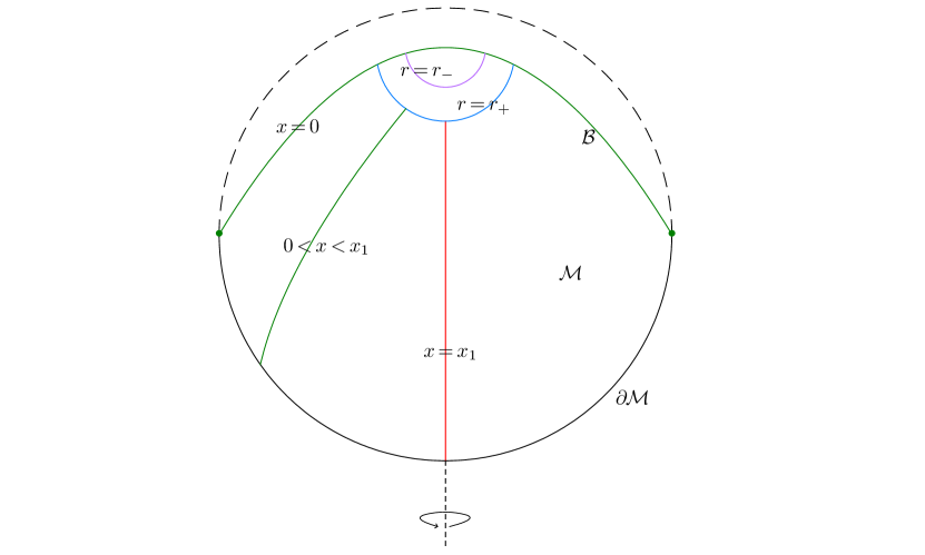
With the four-dimensional charged C-metric spacetime (8) at hand, we can obtain a three-dimensional quantum charged black hole by using the Karch-Randall-Sundrum braneworld formulation. We can consider a configuration where an AdS3 brane with tension is placed in the bulk accelerating spacetime (see Fig. 1). In the notation of Frassino:2022zaz , the total action of the system can be written as
| (20) |
where the bulk action, Gibbons-Hawking-York (GHY) action, and the action of the brane are respectively given by
| (21) |
| (22) |
| (23) |
where is the Ricci scalar of the bulk , is the GHY extrinsic curvature term on the boundary , and is the determinant of the induced metric on the brane . is the four-dimensional Newton constant.
In the KR braneworld model, two patches are glued along the brane obeying the Israel junction condition Israel:1966rt . The tension of the brane is Kudoh:2004ub ; Emparan:2020znc
| (24) |
if we place it at in the bulk spacetime (8). On the brane, we have a three-dimensional induced effective theory of gravitation coupled to electromagnetism, just as in the bulk. The quantum charged black hole mapped from the classical C-metric is
| (25) |
where is given by (11).
Due to the conical deficit of the metric (25), the range of the coordinate is , with111We can expand the metric (11) at with to see this.
| (26) |
However, we can make the azimuthal coordinate have the canonical range via the coordinate transformations
| (27) |
which result in a canonical form of the metric (25) for the quantum charged black hole as
| (28) |
where we can now identify with . Furthermore
| (29) |
with the mass of the black hole and
| (30) |
is a ‘renormalized’ Newton constant. The function
| (31) |
where
| (32) |
expresses the mass in terms of the conical deficit Emparan:1999fd ; Emparan:2020znc ; Kudoh:2004ub . The gauge potential (9) becomes
| (33) |
Solving yields the outer event horizon and inner horizon of the quantum charged black hole on the brane, where .
Comparing the metric function given by Eq. (29) and the gauge potential from Eq. (33) with those of the AdS Reissner-Nordström black hole and the charged BTZ black hole Martinez:1999qi ; Chan:1994qa , we see that the quantum charged black hole is quite similar to the AdS Reissner-Nordström black hole in form. Unlike the BTZ black hole, terms logarithmic in the radial variable do not appear. In the following section, we will explain this by showing that a nonlinear electromagnetic field arises on the brane.
3.2 Quantum backreactions
The metric of the quantum charged black hole (28) solves a deformed semiclassical gravitational field equation
| (34) |
where equals the Einstein term in (1) together with higher-curvature correction terms on the brane, and encodes the extra leading order contributions from the CFT3 holographically dual to the bulk. Using the notation of Frassino:2022zaz , the field equation (34) can be viewed as being derived from the low-energy effective action as
| (35) |
where the first term on the right side of (35)
| (36) |
is the gravitational contribution on the two-brane, with being the electromagnetic tensor on the brane related to the gauge potential (33) and is a function of the electromagnetic invariant. Here we have supposed that the electromagnetic field is minimally coupled with the spacetime curvature.
We note that the Lagrangian of the electromagnetic field on the brane is no longer simply , and a non-linear electromagnetic field coupled with the three-dimensional induced effective gravitation arises. It can be verified that if we set , the equation of motion for the electromagnetic field cannot be satisfied by the gauge potential (33). The non-linearity emerges because the gravitational theory on the brane is modified by higher-curvature terms; in other words, the metric (28) and gauge potential (33) on the brane are induced from (8) and (9) in the bulk, respectively, and the former equations of motion in the bulk are not obeyed anymore. The second term on the right side of (35) is the action of the CFT3, which is holographically defined by the bulk. The explicit expression of this action cannot be given in closed form Emparan:2020znc .
In (36), we can define an effective three-dimensional Newton constant by
| (37) |
where in the last step we have used (30). Following Emparan:2020znc , we can also define an AdS3 length scale on the brane as
| (38) |
using (14) and neglecting terms quadratic in . It is evident that when , i.e., the backreaction from the BCFT3 vanishes, or the brane approaches the boundary. Alternatively, for , which by (24) implies that the tension of the brane vanishes, we have and . With (37) and (38), the brane action (36) can be reformulated as
| (39) |
again neglecting terms quadratic in . From (39), it is evident that we can define the three-dimensional cosmological constant in the effective theory on the brane through the AdS3 scale by
| (40) |
For comparison, we note that in the action (20), we have defined the four-dimensional cosmological constant as
| (41) |
where has the same meaning as in Frassino:2022zaz .
We will first derive the expression of the electromagnetic field based on the action (39). The equation of motion reads
| (42) |
where ′ denotes a derivative with respect to . Substituting the gauge potential (33) yields
| (43) |
where the electromagnetic invariant is . The specific value of the Lagrangian corresponding to the gauge potential (33) is then
| (44) |
where are integration constants. For convenience, we set =0; we note that would be 0 if or . Then we obtain
| (45) |
From (35), we can then obtain the holographic stress tensor in (34)
| (46) | ||||
which can be rearranged as
| (47) |
where
| (48) |
and
| (49) | ||||
By direct calculation we obtain
| (50) | ||||
| (51) |
| (52) |
| (53) |
where for brevity we denote and represents the -th order derivative with respect to . We can thus obtain the trace of the stress-energy tensor as
| (54) | ||||
using (38).
From (54) we can see that for the quantum charged black hole on the brane, the deviation of the matter field from conformal symmetry increases by at least a term of order that is proportional to the electric charge. For the electromagnetic field itself, we know from (50) that the conformal symmetry is also broken due to the backreaction of quantum matter from the in any case, since there is no nonzero constant that can render the stress-energy tensor of the gauge field traceless.
The preceding analysis shows that the quantum charged black hole (28) is induced on the brane, which is the solution to the semiclassical equation of motion (34) on the AdS3 brane. This quantum black hole includes the backreaction from the BCFT3 and corresponds to the classical C-metric solution (8) of the equation of motion (13) in the bulk.
3.3 Thermodynamic quantities
As suggested by Emparan:1999wa ; Emparan:1999fd ; Emparan:2020znc , we can define dimensionless variables related with as
| (55) |
Additionally, we can redefine the charge parameter as
| (56) |
which is dimensionless. Then by combining with (16) we obtain the identities
| (57) |
| (58) |
| (59) |
Since cannot be negative, the parameter defined in (7) is now determined by
| (60) |
where is the sign function.
As a result, in (31) can be rewritten as
| (61) |
where the identities (57)-(58) are used. The mass of the three-dimensional quantum charged black hole, which is related to the conical deficit given by (32), can now be rewritten as
| (62) | ||||
where in the last step we have used the identities (37), which can be further written as
| (63) |
To calculate the entropy of the quantum charged black hole, we first compute the entropy associated with the bulk horizon using the bulk metric given by Eq. (8). The result is
| (64) | ||||
where we denote the bulk entropy as . We can view this entropy as a generalized entropy that incorporates the all orders of backreaction of the quantum matter in the boundary field theory for the quantum black hole on the brane.
For comparison, we note that there can be two other kinds of entropies for the quantum black hole, i.e., the Bekenstein-Hawking entropy and the Wald entropy. Employing Eq. (28), we have the Bekenstein-Hawking area entropy of the quantum charged black hole on the brane as
| (65) |
This area entropy is, however, principally not suitable for the quantum charged black hole on the brane, as the gravitation on the brane is a higher curvature theory, and for the quantum charged black hole, there is also a nonlinear electromagnetic field. Furthermore, as pointed out in Emparan:2020znc for the quBTZ black hole, the three-dimensional area entropy cannot satisfy the thermodynamic first law of the black hole as zero and infinite derivatives emerge when differentiating it with respect to mass.
The Wald entropy in such a sense thus can be an effective candidate entropy for this gravitational theory, which, according to the formula presented in Jacobson:1993vj , is (see appendix A for details)
| (66) |
Note that the Wald entropy given by Eq. (66) is valid only in the small limit up to . However, we aim to obtain an entropy that accounts for the backreaction of the quantum corrections from the boundary field at every order of . As a result, the generalized entropy for the classical four-dimensional black hole can be the only proper candidate mapping to the three-dimensional black hole. As we will see, this entropy indeed satisfies the first law of the quantum charged black hole. We can also obtain the four-dimensional area entropy as the entropy of the quantum black hole by the Euclidean method, just as has been checked by Kudoh:2004ub for the quBTZ black hole. When the backreaction from the CFT3 vanishes (), the difference between the generalized entropy, the area entropy, and the Wald entropy vanishes, yielding
| (67) |
The canonical timelike Killing vector of the quantum charged black hole on the brane is , which gives the temperature of the black hole on the quantum horizon as
| (68) |
To calculate the electric charge of the quantum black hole, we identify the charge computed on the brane with that of the bulk. Using the gauge potential (9) we obtain for the latter
| (69) | ||||
Employing (45), we can also obtain the electric charge of the quantum charged black hole from the nonlinear electromagnetic field on the brane as
| (70) | ||||
Then with the identification of the brane charge and bulk charge, we can solve for the integration constant as
| (71) |
leaving only undetermined in (44) for the gauge field. We also find
| (72) |
for the conjugate electric potential on the brane, where we choose the Killing vector to be , and we have used the gauge potential (33). An alternative way to obtain (72) is to use the gauge potential (9) for the bulk spacetime with the canonical time coordinate in (27).
This is sufficient to show that the first law is satisfied. It is straightforward to verify the relations
| (73) |
| (74) |
are satisfied, where we have expressed thermodynamic quantities in terms of the ‘renormalized’ Newton constant . These two relations ensure that the thermodynamic first law of the quantum charged black hole is
| (75) |
This universal differential relation applies for all parameters for the thermodynamic quantities of the quantum charged black hole.
4 Thermodynamics of quantum charged black holes
We will now investigate the thermodynamic first law and Smarr (energy) relation Smarr:1972kt ; Kastor:2009wy in the extended phase space of the quantum charged black hole, where the cosmological constant is viewed as a dynamical quantity Kubiznak:2016qmn . We shall examine this from three perspectives – bulk, brane, and boundary – in the holographic braneworld model.
4.1 Bulk description
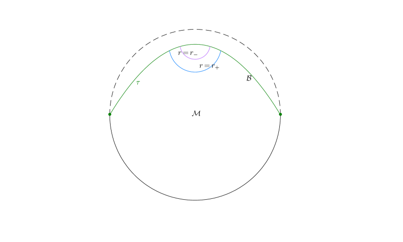
Let’s first consider the thermodynamics of the quantum charged black hole from the bulk perspective. As shown in Fig. 2, the thermodynamic system consists of the bulk black hole and a brane with variable tension, which is a solution of the semiclassical gravitational field equations (34). From the pure bulk perspective of this holographic braneworld setup, we have an bulk spacetime , together with an brane with a tension . The quantum charged black hole on the brane corresponds to the classical solution of the bulk gravity with a brane and encodes all orders of backreaction from the cutoff . In the extended thermodynamic phase space, we can view the four-dimensional cosmological constant and the brane tension as variables. The variation of yields the four-dimensional pressure and its conjugate four-dimensional volume ; the variation of amounts to altering the position of the brane according to the Israel junction conditions. The quantity conjugate to is a quantity with the dimension of area. We shall refer to it as the thermodynamic area of the brane, denoting it as , so that is a work term.
According to (30), (62), (64), and (69), the mass , entropy , and electric charge of the quantum charged black hole from the bulk viewpoint are expressed in terms of the four-dimensional Newton constant as
| (76) | |||||
| (77) | |||||
| (78) |
Furthermore, the thermodynamic pressure of the bulk spacetime is Kubiznak:2016qmn
| (79) |
where in the last step we used (14), (41), and (55). As noted above, the tension (24) of the brane is also a thermodynamic variable and is given in terms of and the backreaction parameter . This backreaction parameter also appears in the expressions for and .
According to the above setup, we can calculate the temperature , electric potential , four-dimensional thermodynamic volume , and the thermodynamic area of the brane as
| (80) | |||||
| (81) | |||||
| (82) | |||||
| (83) | |||||
Here, we have kept the four-dimensional Newton constant fixed, which is a natural setting. The electric potential (81) we obtained here is identical to the one in (72). From the bulk perspective, we find that the thermodynamic first law in the extended phase space, where the four-dimensional cosmological constant and the brane tension are viewed as thermodynamic variables, can be written as
| (84) |
and the Smarr relation
| (85) |
are satisfied. Note that this latter relation can be obtained by Euler’s theorem Frassino:2022zaz . The dimension of the electric charge here is identical to that of the radius , so the coefficient before the term is .
4.2 Brane description
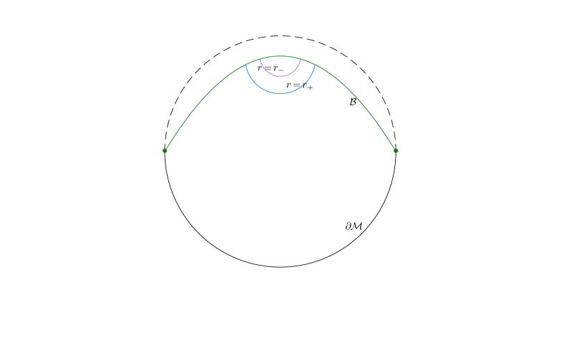
Next, we consider the thermodynamics of the quantum charged black hole from the perspective of the brane (see Fig. 3). In the holographic KR braneworld, the brane intersects the asymptotic boundary of the bulk spacetime at two defects. The brane serves as a holographic renormalization surface for the , and the local higher-curvature gravitational theory on the brane receives backreaction effects from the dual . The UV microscopic degrees of freedom for the are removed by the brane, leaving its central charge to be Emparan:2020znc
| (86) |
where in the last step we used (14) and (37) to express the central charge for the in terms of the radius on the brane and the three-dimensional Newton constant . From (86), we also note that the central charge of the is affected by the backreaction parameter . This suggests that the central charge can be regarded as dynamical Cong:2021fnf ; Cong:2021jgb . However, we will keep the three-dimensional Newton constant fixed222See Susskind:2021nqs for a discussion of a running Newton constant in the context of string/black hole transitions Horowitz:1997jc ; Chen:2021dsw ; Balthazar:2022hno ; Ceplak:2023afb .. Our approach is similar to that employed in Karch:2015rpa ; Sinamuli:2017rhp ; Visser:2021eqk ; Ahmed:2023snm ; Ahmed:2023dnh ; Zhang:2023uay ; Gong:2023ywu ; see Mann:2024sru for a recent review on this topic.
In the extended phase space approach, the thermodynamic pressure corresponds to the three-dimensional cosmological constant in (40). Using (14), (38), and (55), we obtain
| (87) |
which simplifies to when the strength of the backreaction goes to zero. Reexpressing the mass (62), entropy (64), and electric charge (69) of the quantum charged black hole on the brane, we get
| (88) | |||||
| (89) | |||||
| (90) |
in terms of the three-dimensional Newton constant . The thermodynamics of the quantum charged black hole encodes the backreaction of the quantum matter on the .
Keeping as constant, the temperature , electric potential , three-dimensional thermodynamic volume , and three-dimensional chemical potential are
| (91) | |||||
| (92) | |||||
| (93) | |||||
where the temperature and electric potential are the same as their respective bulk counterparts in (80) and (81). This is not difficult to understand, as fixing and yields in (80) and (81), and fixing and yields in (91) and (92), which, according to (55), also gives . From these relationships, it is straightforward to verify that the first law
| (95) |
and the Smarr relation
| (96) |
of the quantum charged black hole are both satisfied, when viewed from the perspective of the brane.
The form of the first law given in (95) is illuminating, as all thermodynamic quantities involved are three-dimensional. These quantities pertain either to the black hole on the brane or to the with a central charge and its conjugate chemical potential. This equation, in fact, represents a mixed form of the first law, comprising both brane quantities and boundary CFT quantities, which is quite similar to the results obtained in Cong:2021fnf ; Cong:2021jgb . In this context, there may be central charge criticality for the quantum charge black hole on the brane; this is a topic we leave for future investigation. It’s also worth noting that in the Smarr relation (96), the electric charge is absent since it is dimensionless in the three-dimensional brane set-up. This result differs from that obtained in Frassino:2015oca for the three-dimensional classical charged BTZ black hole, where the charge is presented in the mass formula via the introduction of a thermodynamic renormalization length scale.
4.3 Boundary description
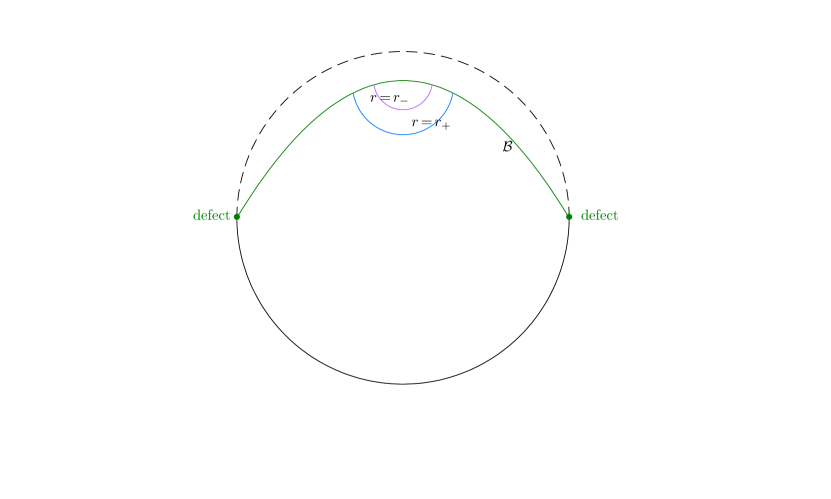
From the bulk perspective, the thermodynamic system we studied comprises a four-dimensional bulk black hole spacetime coupled to a three-dimensional KR brane. From the brane perspective, however, the thermodynamic system transitions to a two-brane black hole spacetime coupled with a three-dimensional . As depicted in Fig. 4, the brane intersects the , resulting in the formation of two defects, each hosting a two-dimensional defect . According to the double holography prescription, this defect , in conjunction with the dynamical higher-curvature gravity on the AdS3 brane, provides a dual description of the thermodynamics on the brane.
Let’s consider the thermodynamics of the quantum charged black hole from the boundary perspective, i.e., from the viewpoint of the defect . The degrees of freedom of the defect are related to the three-dimensional cosmological constant and the Newton constant through the holographic correspondence formula Brown:1986nw
| (97) |
The coefficient here is not crucial and will not affect our results qualitatively. According to the holographic dictionary, the energy, entropy, electric charge, and volume for the defect are respectively given by
| (98) | |||||
| (99) | |||||
| (100) | |||||
| (101) |
where the specific form of the energy is chosen to match (88). The electric charge on the defect is rescaled by Karch:2015rpa ; Visser:2021eqk ; Cong:2021jgb . For the thermodynamic volume of the defect , we can write the boundary metric as Ahmed:2023snm
| (102) |
where is a dynamical conformal factor, implying . We have set in (101).
Based on the above setup, the temperature, two-dimensional pressure, two-dimensional chemical potential, and electric potential are given by
| (103) | |||||
| (104) | |||||
| (105) | |||||
| (106) |
These are respectively conjugate to the entropy, thermodynamic volume, central charge, and electric charge. The full expressions for , and are quite complex and not particularly enlightening, so we choose not to present them explicitly here (see appendix B for details).
To better understand these thermodynamic quantities on the defect , we have expanded all of them in the small limit, i.e., in the small backreaction limit. It’s noticeable that there are no zero order terms in , which implies that all of these quantities vanish when the backreaction of the vanishes. In other words, according to (55), zero backreaction corresponds to vanishing , the limit in which the brane approaches the bulk boundary; in this limit, the tension becomes infinitely large and the defects disappear. Note that we have kept the black hole parameter fixed. This seems to be the only choice, as other quantities , and cannot be fixed in all differential relations. Physically, an invariant means that the radius on the brane is fixed; cf. (55). The first law on the defect reads
| (107) |
where a work term indicates that the energy plays the role of the thermodynamic internal energy. Remarkably, the corresponding integral internal energy formula now contains the electric charge term,
| (108) |
This can be understood in terms of dimensional analysis, as from (100) we know that .
5 Closing remarks
In this paper, we utilized the Karch-Randall-Sundrum braneworld holography formulation to derive a quantum charged black hole on an brane, starting from the C-metric. We analyzed the backreaction effect from the by calculating the holographic stress-energy tensor, revealing that the conformal symmetry property of the nonlinear electromagnetic field on the brane is lost. We derived the mass, generalized entropy, and electric charge, along with their respective conjugate thermodynamic quantities, for the quantum charged black hole. In the extended phase space, we scrutinized the thermodynamic first law and mass (energy) relations for classical and holographic thermodynamics of the black hole from the perspectives of the pure bulk, brane, and boundary, adhering to the double holography prescription.
In the absence of charge, previous results indicated that the quantum black hole resembled the BTZ black hole under a specific parameter setup. However, the quantum charged black hole we derived is not analogous to the charged BTZ black hole in any sense Martinez:1999qi ; Chan:1994qa . As anticipated in Panella:2023lsi , it resembles the AdS Reissner-Nordström black hole, primarily because we have a charge term proportional to . This is a consequence of the nonlinear nature of the electromagnetic field on the brane. In our procedure to obtain this quantum black hole, we selected a brane at a specific position in the original C-metric spacetime. This operation reduced the four-potential electromagnetic field in the bulk to a three-potential. Consequently, the induced gravity on the brane was modified by higher curvature terms, and the induced electromagnetic field on the brane became nonlinear. If the induced electromagnetic field were linear, for instance, a Maxwell field, then the electromagnetic field would match that in the three-dimensional charged BTZ spacetime, as a logarithmic term would appear.
Note that throughout our study, we did not assign specific values to the parameter . The values of correspond to different slicings of the brane. In the uncharged quBTZ scenario, both rotating and non-rotating BTZ black holes can be recovered for , and there exist branches of black holes and black strings for specific values of the combination . By conducting a similar parametric analysis, we discovered that there could also be analogous branches of solutions for quantum charged black objects within a limited mass range. These solutions include a branch with negative mass and a branch representing black strings for specific combinations of parameters . However, in our thermodynamic study of the black hole, does not appear independently in the physical quantities. This implies that our results are universally applicable, regardless of the specific values of .
Indeed, a more detailed analysis of the parameter group is necessary, particularly when our goal is to delve deeper into the chemistry of black holes and the dynamical stability of quantum charged black holes. Beyond the event horizon, a black hole may also have a Cauchy horizon. The stability of this Cauchy horizon for quantum charged black holes is a topic that warrants further clarification. Additionally, studying the relationships between classical black holes in the bulk and on the brane from various perspectives could be a fruitful avenue for future research. This comprehensive approach will provide a deeper understanding of the dynamics and properties of these complex objects on the brane.
Our thermodynamic study of quantum charged black holes was inspired, in part, by the investigations in Frassino:2022zaz on quBTZ black holes. We have found that holographic black hole chemistry Cong:2021fnf ; Ahmed:2023snm can be generalized to a doubly holographic scenario, leading to a number of interesting observations. One is that the Smarr mass relation we derived in this paper, from the brane perspective, does not explicitly contain a charge term, similar to the case of quBTZ black holes. This suggests that, akin to the mass, the electric charge is also dimensionless on the brane. Another point is that the Euler energy formula we obtained from the pure boundary perspective does not contain the and terms. All quantities in this Euler energy formula are derived from the defect field. This discrepancy may stem from differences in the initial setups of the two studies. It is important to note that we have made fixed as an additional necessary condition, which effectively keeps the radius on the brane fixed. This might have affected our results and the differences observed when compared to the referenced work.
Acknowledgements.
This work was supported by the Natural Sciences and Engineering Research Council of Canada and the National Natural Science Foundation of China (Grant Nos. 12365010, 12005080, and 12064018). M. Z. was also supported by the Chinese Scholarship Council Scholarship.Appendix A Wald entropy
For the Lagrangian (39), according to the formula given in Jacobson:1993vj , the Wald entropy is
| (109) | ||||
where , is the trace of the stress-energy tensor , and is the induced metric on a cross section of the black hole horizon. Considering (50)-(54) and (71), we know that
| (110) |
in turn yielding Jacobson:1993vj
| (111) |
for the Wald entropy of the quantum charged black hole up to , where is the metric normal to the black hole horizon, and denotes (28). Explicitly we obtain
| (112) | |||||
| (113) | |||||
Appendix B Explicit expressions of thermodynamic quantities
Here we list the full expressions of the temperature in (103), chemical potential in (105), and electric potential in (106) as
| (114) |
where
| (115) |
where
| (116) |
where
| (117) |
References
- (1) R. Emparan, G.T. Horowitz and R.C. Myers, Exact description of black holes on branes, JHEP 01 (2000) 007 [hep-th/9911043].
- (2) R. Emparan, G.T. Horowitz and R.C. Myers, Exact description of black holes on branes. 2. Comparison with BTZ black holes and black strings, JHEP 01 (2000) 021 [hep-th/9912135].
- (3) R. Emparan, A. Fabbri and N. Kaloper, Quantum black holes as holograms in AdS brane worlds, JHEP 08 (2002) 043 [hep-th/0206155].
- (4) R. Emparan, A.M. Frassino and B. Way, Quantum BTZ black hole, JHEP 11 (2020) 137 [2007.15999].
- (5) A.R. Steif, The Quantum stress tensor in the three-dimensional black hole, Phys. Rev. D 49 (1994) 585 [gr-qc/9308032].
- (6) G. Lifschytz and M. Ortiz, Scalar field quantization on the (2+1)-dimensional black hole background, Phys. Rev. D 49 (1994) 1929 [gr-qc/9310008].
- (7) K. Shiraishi and T. Maki, Quantum fluctuation of stress tensor and black holes in three dimensions, Phys. Rev. D 49 (1994) 5286 [1804.07872].
- (8) M. Banados, C. Teitelboim and J. Zanelli, The Black hole in three-dimensional space-time, Phys. Rev. Lett. 69 (1992) 1849 [hep-th/9204099].
- (9) M. Banados, M. Henneaux, C. Teitelboim and J. Zanelli, Geometry of the (2+1) black hole, Phys. Rev. D 48 (1993) 1506 [gr-qc/9302012].
- (10) C.G. Callan, Jr., S.B. Giddings, J.A. Harvey and A. Strominger, Evanescent black holes, Phys. Rev. D 45 (1992) R1005 [hep-th/9111056].
- (11) A. Strominger, Les Houches lectures on black holes, in NATO Advanced Study Institute: Les Houches Summer School, Session 62: Fluctuating Geometries in Statistical Mechanics and Field Theory, 8, 1994 [hep-th/9501071].
- (12) A. Almheiri, N. Engelhardt, D. Marolf and H. Maxfield, The entropy of bulk quantum fields and the entanglement wedge of an evaporating black hole, JHEP 12 (2019) 063 [1905.08762].
- (13) R. Jackiw, Lower Dimensional Gravity, Nucl. Phys. B 252 (1985) 343.
- (14) C. Teitelboim, Gravitation and Hamiltonian Structure in Two Space-Time Dimensions, Phys. Lett. B 126 (1983) 41.
- (15) A. Almheiri and J. Polchinski, Models of AdS2 backreaction and holography, JHEP 11 (2015) 014 [1402.6334].
- (16) J. Maldacena, D. Stanford and Z. Yang, Conformal symmetry and its breaking in two dimensional Nearly Anti-de-Sitter space, PTEP 2016 (2016) 12C104 [1606.01857].
- (17) J. Engelsöy, T.G. Mertens and H. Verlinde, An investigation of AdS2 backreaction and holography, JHEP 07 (2016) 139 [1606.03438].
- (18) A. Karch and L. Randall, Locally localized gravity, JHEP 05 (2001) 008 [hep-th/0011156].
- (19) J. Garriga and T. Tanaka, Gravity in the brane world, Phys. Rev. Lett. 84 (2000) 2778 [hep-th/9911055].
- (20) L. Susskind, The World as a hologram, J. Math. Phys. 36 (1995) 6377 [hep-th/9409089].
- (21) J.M. Maldacena, The Large N limit of superconformal field theories and supergravity, Adv. Theor. Math. Phys. 2 (1998) 231 [hep-th/9711200].
- (22) S.S. Gubser, I.R. Klebanov and A.M. Polyakov, Gauge theory correlators from noncritical string theory, Phys. Lett. B 428 (1998) 105 [hep-th/9802109].
- (23) E. Witten, Anti-de Sitter space and holography, Adv. Theor. Math. Phys. 2 (1998) 253 [hep-th/9802150].
- (24) S. de Haro, K. Skenderis and S.N. Solodukhin, Gravity in warped compactifications and the holographic stress tensor, Class. Quant. Grav. 18 (2001) 3171 [hep-th/0011230].
- (25) J.L. Cardy, Boundary conformal field theory, hep-th/0411189.
- (26) D.M. McAvity and H. Osborn, Conformal field theories near a boundary in general dimensions, Nucl. Phys. B 455 (1995) 522 [cond-mat/9505127].
- (27) A. Karch and L. Randall, Open and closed string interpretation of SUSY CFT’s on branes with boundaries, JHEP 06 (2001) 063 [hep-th/0105132].
- (28) T. Takayanagi, Holographic Dual of BCFT, Phys. Rev. Lett. 107 (2011) 101602 [1105.5165].
- (29) V.E. Hubeny, M. Rangamani and T. Takayanagi, A Covariant holographic entanglement entropy proposal, JHEP 07 (2007) 062 [0705.0016].
- (30) T. Faulkner, A. Lewkowycz and J. Maldacena, Quantum corrections to holographic entanglement entropy, JHEP 11 (2013) 074 [1307.2892].
- (31) A. Lewkowycz and J. Maldacena, Generalized gravitational entropy, JHEP 08 (2013) 090 [1304.4926].
- (32) N. Engelhardt and A.C. Wall, Quantum Extremal Surfaces: Holographic Entanglement Entropy beyond the Classical Regime, JHEP 01 (2015) 073 [1408.3203].
- (33) A. Almheiri, R. Mahajan, J. Maldacena and Y. Zhao, The Page curve of Hawking radiation from semiclassical geometry, JHEP 03 (2020) 149 [1908.10996].
- (34) H.Z. Chen, R.C. Myers, D. Neuenfeld, I.A. Reyes and J. Sandor, Quantum Extremal Islands Made Easy, Part I: Entanglement on the Brane, JHEP 10 (2020) 166 [2006.04851].
- (35) H.Z. Chen, R.C. Myers, D. Neuenfeld, I.A. Reyes and J. Sandor, Quantum Extremal Islands Made Easy, Part II: Black Holes on the Brane, JHEP 12 (2020) 025 [2010.00018].
- (36) S. Ryu and T. Takayanagi, Holographic derivation of entanglement entropy from AdS/CFT, Phys. Rev. Lett. 96 (2006) 181602 [hep-th/0603001].
- (37) S. Ryu and T. Takayanagi, Aspects of Holographic Entanglement Entropy, JHEP 08 (2006) 045 [hep-th/0605073].
- (38) H. Geng, A. Karch, C. Perez-Pardavila, S. Raju, L. Randall, M. Riojas et al., Jackiw-Teitelboim Gravity from the Karch-Randall Braneworld, Phys. Rev. Lett. 129 (2022) 231601 [2206.04695].
- (39) H. Kudoh and Y. Kurita, Thermodynamics of four-dimensional black objects in the warped compactification, Phys. Rev. D 70 (2004) 084029 [gr-qc/0406107].
- (40) A.M. Frassino, J.F. Pedraza, A. Svesko and M.R. Visser, Higher-Dimensional Origin of Extended Black Hole Thermodynamics, Phys. Rev. Lett. 130 (2023) 161501 [2212.14055].
- (41) J.F. Plebanski and M. Demianski, Rotating, charged, and uniformly accelerating mass in general relativity, Annals Phys. 98 (1976) 98.
- (42) W. Israel, Singular hypersurfaces and thin shells in general relativity, Nuovo Cim. B 44S10 (1966) 1.
- (43) M. Appels, R. Gregory and D. Kubiznak, Thermodynamics of Accelerating Black Holes, Phys. Rev. Lett. 117 (2016) 131303 [1604.08812].
- (44) N. Abbasvandi, W. Cong, D. Kubiznak and R.B. Mann, Snapping swallowtails in accelerating black hole thermodynamics, Class. Quant. Grav. 36 (2019) 104001 [1812.00384].
- (45) R. Gregory and A. Scoins, Accelerating Black Hole Chemistry, Phys. Lett. B 796 (2019) 191 [1904.09660].
- (46) M. Appels, R. Gregory and D. Kubiznak, Black Hole Thermodynamics with Conical Defects, JHEP 05 (2017) 116 [1702.00490].
- (47) A. Anabalón, M. Appels, R. Gregory, D. Kubizňák, R.B. Mann and A. Ovgün, Holographic Thermodynamics of Accelerating Black Holes, Phys. Rev. D 98 (2018) 104038 [1805.02687].
- (48) L. Randall and R. Sundrum, A Large mass hierarchy from a small extra dimension, Phys. Rev. Lett. 83 (1999) 3370 [hep-ph/9905221].
- (49) L. Randall and R. Sundrum, An Alternative to compactification, Phys. Rev. Lett. 83 (1999) 4690 [hep-th/9906064].
- (50) R. Emparan, J.F. Pedraza, A. Svesko, M. Tomašević and M.R. Visser, Black holes in dS3, JHEP 11 (2022) 073 [2207.03302].
- (51) E. Panella and A. Svesko, Quantum Kerr-de Sitter black holes in three dimensions, JHEP 06 (2023) 127 [2303.08845].
- (52) R. Emparan, A.M. Frassino, M. Sasieta and M. Tomašević, Holographic complexity of quantum black holes, JHEP 02 (2022) 204 [2112.04860].
- (53) B. Chen, Y. Liu and B. Yu, Holographic complexity of rotating quantum black holes, JHEP 01 (2024) 055 [2307.15968].
- (54) C.V. Johnson and R. Nazario, Specific Heats for Quantum BTZ Black Holes in Extended Thermodynamics, 2310.12212.
- (55) A.M. Frassino, J.F. Pedraza, A. Svesko and M.R. Visser, Reentrant phase transitions of quantum black holes, 2310.12220.
- (56) S.A. Hosseini Mansoori, J.F. Pedraza and M. Rafiee, Criticality and thermodynamic geometry of quantum BTZ black holes, 2403.13063.
- (57) S.-P. Wu and S.-W. Wei, Thermodynamical Topology of Quantum BTZ Black Hole, 2403.14167.
- (58) M. Kolanowski and M. Tomašević, Singularities in 2D and 3D quantum black holes, JHEP 12 (2023) 102 [2310.06014].
- (59) V. Cardoso, J.a.L. Costa, K. Destounis, P. Hintz and A. Jansen, Quasinormal modes and Strong Cosmic Censorship, Phys. Rev. Lett. 120 (2018) 031103 [1711.10502].
- (60) D. Kastor, S. Ray and J. Traschen, Enthalpy and the Mechanics of AdS Black Holes, Class. Quant. Grav. 26 (2009) 195011 [0904.2765].
- (61) M. Cvetic, G.W. Gibbons, D. Kubiznak and C.N. Pope, Black Hole Enthalpy and an Entropy Inequality for the Thermodynamic Volume, Phys. Rev. D 84 (2011) 024037 [1012.2888].
- (62) B.P. Dolan, Pressure and volume in the first law of black hole thermodynamics, Class. Quant. Grav. 28 (2011) 235017 [1106.6260].
- (63) D. Kubiznak and R.B. Mann, P-V criticality of charged AdS black holes, JHEP 07 (2012) 033 [1205.0559].
- (64) S.-W. Wei, Y.-X. Liu and R.B. Mann, Repulsive Interactions and Universal Properties of Charged Anti–de Sitter Black Hole Microstructures, Phys. Rev. Lett. 123 (2019) 071103 [1906.10840].
- (65) D. Kubiznak, R.B. Mann and M. Teo, Black hole chemistry: thermodynamics with Lambda, Class. Quant. Grav. 34 (2017) 063001 [1608.06147].
- (66) Y. Xiao, Y. Tian and Y.-X. Liu, Extended Black Hole Thermodynamics from Extended Iyer-Wald Formalism, Phys. Rev. Lett. 132 (2024) 021401 [2308.12630].
- (67) W. Kinnersley and M. Walker, Uniformly accelerating charged mass in general relativity, Phys. Rev. D 2 (1970) 1359.
- (68) C. Martinez, C. Teitelboim and J. Zanelli, Charged rotating black hole in three space-time dimensions, Phys. Rev. D 61 (2000) 104013 [hep-th/9912259].
- (69) K.C.K. Chan and R.B. Mann, Static charged black holes in (2+1)-dimensional dilaton gravity, Phys. Rev. D 50 (1994) 6385 [gr-qc/9404040].
- (70) W. Cong, D. Kubiznak and R.B. Mann, Thermodynamics of AdS Black Holes: Critical Behavior of the Central Charge, Phys. Rev. Lett. 127 (2021) 091301 [2105.02223].
- (71) M.B. Ahmed, W. Cong, D. Kubizňák, R.B. Mann and M.R. Visser, Holographic Dual of Extended Black Hole Thermodynamics, Phys. Rev. Lett. 130 (2023) 181401 [2302.08163].
- (72) H. Weyl, The theory of gravitation, Annalen Phys. 54 (1917) 117.
- (73) T. Levi-Civita, T. levi-civita, atti accad. naz. lincei cl. sci. fis. mat. nat. rend. 27, 343 (1918)., Atti Accad. Naz. Lincei Cl. Sci. Fis. Mat. Nat. Rend. 27 (1918) 343.
- (74) E. Newman and L. Tamburino, New approach to einstein’s empty space field equations, Journal of Mathematical Physics 2 (1961) 667.
- (75) I. Robinson, I. robinson and a. trautman, proc. r. soc. london a265, 463 (1962), Proc. R. Soc. London 265 (1962) 463.
- (76) R.B. Mann, Pair production of topological anti-de Sitter black holes, Class. Quant. Grav. 14 (1997) L109 [gr-qc/9607071].
- (77) K. Hong and E. Teo, A New form of the C metric, Class. Quant. Grav. 20 (2003) 3269 [gr-qc/0305089].
- (78) T. Jacobson, G. Kang and R.C. Myers, On black hole entropy, Phys. Rev. D 49 (1994) 6587 [gr-qc/9312023].
- (79) L. Smarr, Mass formula for Kerr black holes, Phys. Rev. Lett. 30 (1973) 71.
- (80) W. Cong, D. Kubiznak, R.B. Mann and M.R. Visser, Holographic CFT phase transitions and criticality for charged AdS black holes, JHEP 08 (2022) 174 [2112.14848].
- (81) L. Susskind, Black Hole-String Correspondence, 2110.12617.
- (82) G.T. Horowitz and J. Polchinski, Selfgravitating fundamental strings, Phys. Rev. D 57 (1998) 2557 [hep-th/9707170].
- (83) Y. Chen, J. Maldacena and E. Witten, On the black hole/string transition, JHEP 01 (2023) 103 [2109.08563].
- (84) B. Balthazar, J. Chu and D. Kutasov, On small black holes in string theory, JHEP 03 (2024) 116 [2210.12033].
- (85) N. Čeplak, R. Emparan, A. Puhm and M. Tomašević, The correspondence between rotating black holes and fundamental strings, JHEP 11 (2023) 226 [2307.03573].
- (86) A. Karch and B. Robinson, Holographic Black Hole Chemistry, JHEP 12 (2015) 073 [1510.02472].
- (87) M. Sinamuli and R.B. Mann, Higher Order Corrections to Holographic Black Hole Chemistry, Phys. Rev. D 96 (2017) 086008 [1706.04259].
- (88) M.R. Visser, Holographic thermodynamics requires a chemical potential for color, Phys. Rev. D 105 (2022) 106014 [2101.04145].
- (89) M.B. Ahmed, W. Cong, D. Kubiznak, R.B. Mann and M.R. Visser, Holographic CFT phase transitions and criticality for rotating AdS black holes, JHEP 08 (2023) 142 [2305.03161].
- (90) M. Zhang and J. Jiang, Bulk-boundary thermodynamic equivalence: a topology viewpoint, JHEP 06 (2023) 115 [2303.17515].
- (91) T.-F. Gong, J. Jiang and M. Zhang, Holographic thermodynamics of rotating black holes, JHEP 06 (2023) 105 [2305.00267].
- (92) R.B. Mann, Recent Developments in Holographic Black Hole Chemistry, JHAP 4 (2024) 1 [2403.02864].
- (93) A.M. Frassino, R.B. Mann and J.R. Mureika, Lower-Dimensional Black Hole Chemistry, Phys. Rev. D 92 (2015) 124069 [1509.05481].
- (94) J.D. Brown and M. Henneaux, Central Charges in the Canonical Realization of Asymptotic Symmetries: An Example from Three-Dimensional Gravity, Commun. Math. Phys. 104 (1986) 207.