GCV-Turbo: End-to-end Acceleration of GNN-based Computer Vision Tasks on FPGA

Abstract

Graph neural networks (GNNs) have recently empowered various novel computer vision (CV) tasks. In GNN-based CV tasks, a combination of CNN layers and GNN layers or only GNN layers are employed. This paper introduces GCV-Turbo, a domain-specific accelerator on FPGA for end-to-end acceleration of GNN-based CV tasks. GCV-Turbo consists of two key components: (1) a novel hardware architecture optimized for the computation kernels in both CNNs and GNNs using the same set of computation resources. (2) a PyTorch-compatible compiler that takes a user-defined model as input, performs end-to-end optimization for the computation graph of a given GNN-based CV task, and produces optimized code for hardware execution. The hardware architecture and the compiler work synergistically to support a variety of GNN-based CV tasks. We implement GCV-Turbo on a state-of-the-art FPGA and evaluate its performance across six representative GNN-based CV tasks with diverse input data modalities (e.g., image, human skeleton, point cloud). Compared with state-of-the-art CPU (GPU) implementations, GCV-Turbo achieves an average latency reduction of $68.4\times$ ($4.1\times$) on these six GNN-based CV tasks. Moreover, GCV-Turbo supports the execution of the standalone CNNs or GNNs, achieving performance comparable to that of state-of-the-art CNN (GNN) accelerators for widely used CNN-only (GNN-only) models.

I Introduction

Graph Neural Networks (GNNs) are playing an increasingly important role in various computer vision (CV) tasks [1, 2]. Figure 1 demonstrates several examples. These applications utilize the combined power of convolution in CNN layers and message passing in GNN layers. This has given rise to a new domain called GNN-based CV: CV tasks that utilize a combination of CNN and GNN layers (e.g., iteratively interleaving CNN layer and GNN layer) or rely solely on GNN layers.

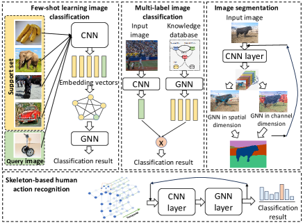
Figure 1: Examples of GNN-based CV tasks [3, 4, 5, 6]

GNN layers have gained widespread adoption in CV tasks because: (1) Firstly, GNN layers facilitate label-efficient image classification. Training standalone CNN [7] or vision transformer (ViT) [8] typically requires a substantial number of labeled images. For instance, achieving high accuracy with ViTs requires over 300 million labeled images. In contrast, researchers have devised label-efficient few-shot learning techniques [3] that combine GNN layers and CNN layers, requiring only a small number of labeled images. (2) Secondly, GNN layers can naturally handle non-Euclidean data structures in diverse CV tasks, such as point clouds [9, 10, 11], 3D meshes [12, 13]. In contrast, the convolution of the CNN layer and the multi-head self-attention (MSA) of ViTs are designed for regular grids and cannot be directly employed with non-Euclidean data structures. For example, convolution operates on 2D grids, and MSA [8] relies on positional encodings on 2D grids. (3) Thirdly, the message passing of GNN layers excel in relation learning for various CV tasks, allowing them to understand complex object relationships. In video action recognition, a CNN [14] detects multiple objects, while GNN layers [15] are employed to capture object relationships.

Given this domain’s expanding scope and future relevance, there is an urgent need for end-to-end acceleration for these GNN-based CV tasks. For example, in autonomous driving, low latency inference is crucial to ensure safety. Nevertheless, it poses significant challenges: while there are various CNN accelerators [16, 17, 18, 19, 20, 21, 22] or GNN accelerators [23, 24, 25, 26, 27, 28, 29, 30] proposed. The hardware architecture of these CNN or GNN accelerators is optimized solely for one layer type, which is inefficient for the end-to-end acceleration of GNN-based CV. For example, CNN accelerators [16, 17, 18, 19, 20, 21, 22] are not efficient for message passing in GNN layers while GNN accelerators achieve suboptimal performance on convolution operation of CNN layers. While we can potentially combine a CNN accelerator and a GNN accelerator for GNN-based CV, it can lead to sub-optimal performance due to resource underutilization. For example, when executing a CNN layer, the GNN accelerator will be idle and vice versa. Another possible solution is to build FPGA bitstreams for CNN and GNN layers, respectively. However, this requires dynamic reconfiguration of FPGA for executing a model, which can incur significant latency and is not suitable for latency-sensitive applications. (2) GNN-based CV model has a mixture of dataflow because the GNN layer and CNN layer can be interleaved but have very different data layouts. Existing compilers and hardware architectures of the aforementioned CNN or GNN accelerators are not optimized for this dataflow mixture, which can potentially lead to large overhead in transforming data layouts between two types of layers. Coordinating the data layout between the CNN and GNN layers requires non-trivial compiler-hardware codesign. (3) General purpose processors (CPU, GPGPU) are not well-suited for low-latency inference of GNN-based CV. Because they have complex cache hierarchies leading to large and unpredictable memory access latency, unsuitable for latency-sensitive applications. Given that there are no existing accelerators for GNN-based CV, the execution of existing GNN-based CV [3, 4, 5, 6, 31, 10] rely on CPU/GPU, leading to suboptimal performance. (4) Moreover, autonomous driving systems execute various CV tasks including non-GNN CV. Therefore, an accelerator should not only achieve high performance for GNN-based CV, but also not sacrifice much performance for tasks that utilize standalone CNNs or GNNs.

To address the above challenges, we propose GCV-Turbo, a domain-specific accelerator on FPGA for end-to-end acceleration of GNN-based CV. Unlike existing CNN and GNN accelerators, the architecture design of GCV-Turbo employs the resource sharing strategy that different computation kernels in CNNs and GNNs share the same computation resources for improved resource utilization. Moreover, the compiler not only optimizes CNN layers or GNN layers but also performs end-to-end optimizations for the mixture dataflow of CNN and GNN layers. Our main contributions are:

• We propose GCV-Turbo, the first domain-specific accelerator for end-to-end acceleration of GNN-based CV tasks.

• We design a novel hardware architecture with a flexible data path and memory organization capable of executing various computation kernels in CNN and GNN layers using the same set of hardware resources.

• We develop a customized compiler for end-to-end optimizations that reduces inference latency of GNN-based CV, including (1) optimizations for data manipulation between CNN layers and GNN layers, (2) data layout centric mapping, (3) sparsity-aware computation primitive mapping.

• We implement the hardware design on a state-of-the-art FPGA board, Alveo U250. Evaluated on six representative GNN-based CV tasks, GCV-Turbo achieves average latency reduction of $68.4\times$ and $4.1\times$ compared with the state-of-the-art implementations on CPU and GPU, respectively.

• We compare GCV-Turbo with state-of-the-art CNN and GNN accelerators. GCV-Turbo demonstrates performance comparable to CNN DSAs for CNN-only models (with a speedup of $0.88$ to $0.93\times$), and to GNN accelerators for GNN-only models (with a speedup of $1.03$ to $1.25\times$).

To the best of our knowledge, GCV-Turbo is the first hardware-compiler codesign capable of executing both CNN and GNN layers, optimized for the end-to-end acceleration of GNN-based CV, and also maintaining good performance on tasks that utilize standalone CNN or GNN.

II Background

II-1 GNN-based Computer Vision Tasks

Figure 1 shows several representative GNN-CV tasks. We conduct an experimental study to understand the challenges of accelerating GNN-based CV: (1) In CNN-based CV tasks, both CNN and GNN layers can be computationally extensive. Moreover, the computation workloads of CNN/GNN layers vary in tasks ranging from $2\%-100\%$ (Figure 2). Directly combining a CNN accelerator and a GNN accelerator can lead to severe hardware underutilization. For example, the GNN accelerator will be idle when executing a CNN layer. This underutilization can increase the inference latency. (2) In GNN-based CV tasks, the CNN layer and GNN layer have very different data layouts for input and output data. Moreover, the CNN layer and GNN layer can be interleaved (which is for better feature fusion in GNN-based CV. See image segmentation and skeleton-based human action recognition in Figure 1). Switching the data layout (including permute(), transpose(), and other indexing functions) between the CNN layer and the GNN layer can lead to significant overhead, taking $1\%-15\%$ execution time on a state-of-the-art GPU platform (Figure 2). This can be more severe on embedded platforms with limited memory bandwidth since layout transformation is memory-bound. (3) General purpose processors (CPU, GPU) are hard to achieve low-latency inference for GNNs [23, 26, 25], because GNN has irregular data access patterns and memory access patterns. Due to the complex cache hierarchy, CPU and GPU have low efficiency [23, 26, 25] for executing GNNs.

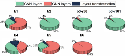
Figure 2: Breakdown analysis of GNN-based CV tasks (b1—-b6—) on state-of-the-art GPU (RTX A5000). The details of the models and datasets are elaborated in Section VI.

II-2 Domain Specific Accelerators

A multitude of domain-specific accelerators (DSAs) [16, 17, 18, 19, 20, 21] have been proposed to accelerate CNNs. However, these CNN-specific DSAs have challenges in both hardware design and compiler implementation when it comes to executing GNN-based CV tasks, as elaborated in Section I. Recently, a DSA known as GraphAGILE [32] has emerged to accelerate GNNs. Unfortunately, the GraphAGILE compiler does not accommodate CNNs, which is crucial for GNN-based CV tasks. Moreover, GraphAGILE does not explore the data sparsity in GNNs, which can result in suboptimal performance when applied to GNN-based CV tasks. Meanwhile, there exist other accelerators [33] designed for specific GNN-based CV tasks. RFC-HyPGCN [33] specializes in running 2S-AGCN [34] for human-skeleton-based action recognition, while Pointacc [35] is tailored to accelerate several GNNs utilized in point cloud applications. In summary, prior research efforts either (1) design DSAs exclusively for CNNs or GNNs, or (2) design accelerators optimized for specific GNN-based CV tasks.

III Overview

III-A Problem Definition

Our objective is to perform end-to-end inference acceleration of GNN-based CV tasks. End-to-end acceleration refers to reducing the inference latency of a GNN-based CV task, which is duration from when the input data is given to the time when the inference result is obtained. This includes data loading from external memory, executing all the layers of the model on the accelerator, and storing the results in the external memory. To this end, we propose a compiler-hardware codesign. The compilation is an offline process. The GCV-Turbo compiler takes a user-defined model (written in PyTorch [36] and PyTorch Geometric [37]) as input and generates optimized code for hardware execution. The GCV-Turbo hardware design has a fixed architecture that execute various models without reconfiguring the FPGA. This is important for many real-world systems, such as autonomous driving, which execute various models for various data modality. We target latency-sensitive applications such as autonomous driving, where inference latency should be low to ensure safety.

III-B Overview of GCV-Turbo

Figure 3 illustrates the overview of GCV-Turbo: (1) Compiler: It is executed on the host processor. The input parser generates the intermediate representation (computation graph) from the given input model. The computation graph or intermediate representation is the high-level representation of the input model with each node representing a layer and each arrow representing the data dependency. Then, compiler performs five-step compilation to map the input model onto the hardware accelerator. We apply several compiler optimizations (Section V-C) for GNN-based CV. Finally, the compiler generates an instruction sequence for hardware execution. (2) Application processing unit (APU): The APU of FPGA [38] takes the instruction sequence as input and launches the workload of inference on the hardware accelerator. (3) Hardware accelerator: The hardware accelerator executes the computation tasks scheduled by APU.

Hardware design: As discussed in Section I, existing CNN or GNN accelerators suffer from inefficiency when handling GNN-based CV tasks. To tackle this challenge, we identify fundamental computation primitives (Section IV-A) capable of representing computation kernels in both GNNs and CNNs. Subsequently, we design a flexible data path and memory organization for efficient execution of these computation primitives within our hardware design. This enables our accelerator to support both CNNs and GNNs. Meanwhile, our proposed accelerator incorporates an instruction set (Section IV-B) providing software-like programmability. Note that our hardware design employs resource sharing strategy (Section IV) such that the computation kernels of CNN and GNN share the same set of computation resources.

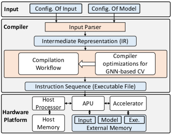
Figure 3: Overview of GCV-Turbo

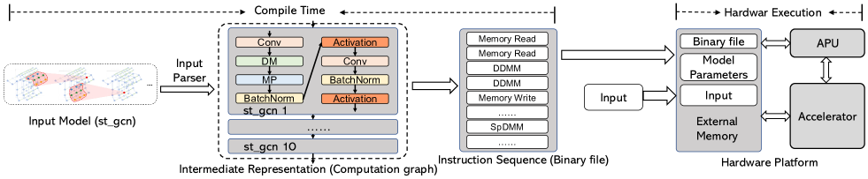
Figure 4: Workflow of GCV-Turbo using the skeleton-based human action recognition [6] as an example.

Compiler design: Designing a compiler to support GNN-based CV is not merely merging separate compiler optimization for CNNs and GNNs. Instead, it needs the end-to-end optimization of the computation graph of a GNN-based CV model. Because: (1) a GNN-based CV task often comprises both CNN and GNN layers, and these layers can be interwoven (e.g., [6]). (2) These two layer types exhibit different data layouts and memory access patterns. Without careful dataflow optimization, switching data layouts can lead to substantial overhead and increased memory access latency. To address this challenge, we devise a five-step compilation workflow (Section V) with various compiler optimizations for GNN-based CV (Section V-C).

Workflow: The workflow is illustrated in Figure 4. At compile time, the compiler takes the user-defined model as input and produces the intermediate representation (i.e., computation graph). The compiler then performs a five-step compilation to generate an instruction sequence stored in a binary file. During hardware execution, the APU reads the binary file and schedules the computation tasks on the hardware accelerator.

Experimental study: We conduct the comprehensive experimental study on six representative GNN-based CV tasks (Section VII-A). Because these tasks (1) cover various use cases and data modalities (See Table III) in real-world applications, such as autonomous driving, (2) cover various computational characteristics of GNN-based CV (See Figure 2), such as varying portions of CNN/GNN layers, varying patterns of layout transformation between CNN and GNN layers. Evaluating these tasks, we expect GCV-Turbo to perform similarly on a broad range of GNN-based CV tasks.

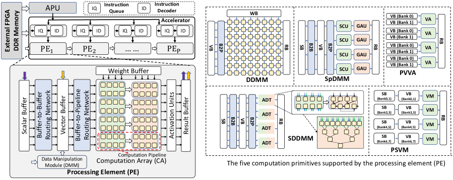
Figure 5: Architecture of hardware accelerator, and the basic computation primitives supported by a PE.

IV Hardware Architecture

As illustrated in Figure 5, GCV-Turbo has a unified hardware architecture that efficiently executes various computation primitives (Section IV-A) in CNNs and GNNs. The accelerator has multiple parallel processing elements (PEs), with each having an Instruction Queue (IQ) and an Instruction Decoder (ID). Each PE has a computation array (CA) with $p_{\text{ca}}^{2}$ computation units. Each computation unit executes the basic arithmetic operations. Each PE has a Scalar Buffer (SB), a Vector Buffer (VB), a Weight Buffer (WB), and a Result Buffer (RB). Each Buffer (SB/VB/WB/RB) has $p_{\text{ca}}$ memory banks. Each bank can output $p_{\text{ca}}$ data per cycle. There are two all-to-all data routing networks – Buffer-to-Buffer (B2B) and Buffer-to-Pipeline (B2P) Routing Network. Data Manipulation Module performs transformations of data layout between different layers (e.g., CNN layer and GNN layer).

Resource sharing: Note that in a PE, different computation primitives share the same set of computation units, data buffers, and routing networks. See more details in Section IV-A. This increases the resource utilization for executing a GNN-based CV task. For resource sharing, it only requires extra extra wire connections and hardware multiplexers for selecting data path for different computation primitives, which incur small hardware cost (See Section VI).

IV-A Computation Primitives

In GNN-based CV tasks, we identify five basic computation primitives (Figure 5), including dense-dense matrix multiplication (DDMM), sparse-dense matrix multiplication (SpDMM), sampled dense-dense matrix multiplication (SDDMM), parallel scalar-vector multiplication (PSVM), and parallel vector-vector addition (PVVA). Each layer can be mapped to these basic computation primitives. The PE has a flexible architecture to support these computation primitives. Each PE maintains hardware multiplexers to select the data path for executing various primitives. Switching among primitives incurs one clock cycle overhead. For simplicity, the input to a computation primitive are two matrices denoted as $\mathbf{X}\in\mathbb{R}^{s_{1}\times s_{2}}$ and $\mathbf{Y}\in\mathbb{R}^{s_{2}\times s_{3}}$. The output matrix is denoted as $\mathbf{Z}\in\mathbb{R}^{s_{1}\times s_{3}}$.

DDMM: DDMM executes $\mathbf{X}\times\mathbf{Y}$, and views $\mathbf{X}$ and $\mathbf{Y}$ as dense matrices. To this end, the computation array is organized as a 2-D systolic array (See Figure 5) with localized interconnection. $\mathbf{X}$ and $\mathbf{Y}$ are stored in VB and WB, respectively. Different from traditional 2-D systolic arrays, DDMM incorporates a B2P routing network for shuffling the position of input vectors (rows of $\mathbf{X}$), which supports data layout transformation between CNN layer and GNN layer (See Section V-C). DDMM can execute $p_{\text{ca}}\times p_{\text{ca}}$ multiply-accumulate (MAC) operations in each clock cycle.

SpDMM: SpDMM executes $\mathbf{X}\times\mathbf{Y}$ where $\mathbf{X}$ is a sparse matrix. The computation array is organized as multiple pipelines with each having a Scatter Unit (SCU) and a Gather Unit (GAU). Each non-zero element in $\mathbf{X}$ is represented using a three-tuple $(src,dst,val)$, denoting row index, column index, and value, respectively. The execution follows the scatter-gather paradigm [39, 40] as shown in Algorithm 1. Executing $\mathbf{X}\times\mathbf{Y}$ takes $l_{\text{SpDMM}}$ clock cycles: ${\textstyle l_{\text{SpDMM}}(\mathbf{X},\mathbf{Y})=\lceil\frac{Nonz(\mathbf{X})}{p_{\text{ca}}/2}\rceil\times\lceil\frac{s_{3}}{p_{\text{ca}}}\rceil}$ where $\textstyle{Nonz(\mathbf{X})}$ denotes the number of non-zeros in $\mathbf{X}$.

Algorithm 1 SpDMM using Scatter-Gather paradigm

while not done do $\triangleright$ Pipelined Execution

    for each $(src,dst,val)\in\mathbf{X}$ in SB do $\triangleright$ Data Fetching

         Route $(src,dst,val)$ from SB to VB $\triangleright$ B2B

         Fetch row $src$ of $\mathbf{Y}$: $\mathbf{Y}[src]$ from VB

         Form input pair {$\mathbf{Y}[src]$, $(src,dst,val)$}

         Route the input pair to pipeline $dst\%(p_{\text{ca}}/2)$ $\triangleright$ B2P     

    for each input pair {$\mathbf{Y}[src]$, $(src,dst,val)$}  do

         Produce $\mathbf{u}\leftarrow$ $val\times\mathbf{Y}[src]$ $\triangleright$ Scatter Unit (SCU)

         Update $\mathbf{Z}[dst]+=\mathbf{u}$ $\triangleright$ Gather Unit (GAU)     

SDDMM: SDDMM executes $\mathbf{Z}=\mathbf{A}\odot(\mathbf{X}\mathbf{Y})$ $(\mathbf{A}\in\mathbb{R}^{s_{1}\times s_{3}})$, where $\odot$ is the element-wise multiplication. $\mathbf{A}$ is a sampling matrix where each element is either $1$ or $0$ to sample results from $\mathbf{X}\mathbf{Y}$. For example, if $\mathbf{A}[i][j]=1$, then $\mathbf{Z}[i][j]=\langle\mathbf{X}[i],\mathbf{Y}[j]\rangle$ where $\langle,\rangle$ denotes vector inner product operator. If $\mathbf{A}[i][j]=0$, $\mathbf{Z}[i][j]=0$. Each computation pipeline is organized as an adder tree (ADT). The execution of SDDMM is shown in Algorithm 2. Executing $\mathbf{A}\odot(\mathbf{X}\mathbf{Y})$ takes $l_{\text{SDDMM}}$ clock cycles, where ${\textstyle l_{\text{SDDMM}}(\mathbf{X},\mathbf{Y})=\lceil\frac{Nonz(\mathbf{X})}{p_{\text{ca}}/2}\rceil\times\lceil\frac{s_{2}}{p_{\text{ca}}}\rceil}$.

Algorithm 2 Sampled dense-dense matrix multiplication

while not done do $\triangleright$ Pipelined Execution

    for each $(src,dst)\in\mathbf{A}$ in SB do $\triangleright$ Data Fetching

         Route $(src,dst)$ from SB to VB $\triangleright$ B2B

         Fetch $\mathbf{X}[src]$ and $\mathbf{Y}[dst]$ from VB

         Form input pair {$\mathbf{X}[src]$, $\mathbf{Y}[dst]$}

         Route the input pair to a pipeline $\triangleright$ B2P     

    for each input pair do $\triangleright$ Computation

         Update $\mathbf{Z}[src][dst]+=\langle\mathbf{X}[src],\mathbf{Y}[dst]\rangle$ $\triangleright$ ADT     

PSVM: To execute PSVM, the computation array is organized as $p_{\text{ca}}/2$ independent pipelines. Each pipeline has a vector multiplier (VM) to execute the multiplication between a scalar and a vector of length $p_{\text{ca}}$. A PE can execute $p_{\text{ca}}^{2}/2$ multiply operations per clock cycle. PSVM can be used to perform matrix-vector multiplication.

PVVA: To execute PVVA, for $p_{\text{ca}}/2$ independent pipelines, each pipeline has a vector adder (VA) to execute the vector addition between two vectors of length $p_{\text{ca}}$. A PE can execute $p_{\text{ca}}^{2}/2$ addition operations per cycle. PVVA can be used to execute matrix addition.

IV-B Instruction Set

We develop a customized instruction set, including computation instructions, memory read/write instructions. (1) Computation Instructions includes the instruction for each computation primitives (e.g., DDMM instruction). Each instruction contains the meta data (e.g., matrix size) of the corresponding computation primitive. The Instruction Decoder decodes the instruction and generates control signal for the PE to execute the computation primitives in pipelined manner. Memory Read/Write Instructions launch the data transactions between the on-chip buffer and the external memory.

V Compiler

Existing compilers for CNN or GNN accelerator [16, 17, 18, 19, 20, 21, 22, 41] support only one type of model (CNN or GNN). In contrast, GCV-Turbo offers an end-to-end compilation/optimization workflow for GNN-based CVs. For a given input model developed using PyTorch, the Input Parser converts it into an intermediate representation (Section V-A), which serves as the computation graph underlying the inference process. The compiler then performs a five-step compilation (Section V-B) to generate an instruction sequence. Especially, we perform a number of specific optimizations (Section V-C) for GNN-based CV tasks: including (1) data manipulation (DM) layer generation, (2) layer fusion for DM layer, (3) uniform mapping, (4) data layout centric mapping, and (5) sparsity-aware primitive mapping. Our compiler utilizes the infrastructure of TVM framework [42]. Based on it, we develop our own input parser, intermediate representation, compilation workflow, and compiler optimizations.

V-A Intermediate Representation

We develop the intermediate representation (IR) for the following set of computation layers in GNN-based CV tasks:

Convolutional (Conv) Layer: The input $\mathfrak{F}_{\text{in}}$ has $c_{\text{in}}$ feature maps (channels), each having a size of $h_{\text{in}}\times w_{\text{in}}$. The output $\mathfrak{F}_{\text{out}}$ has $c_{\text{out}}$ feature maps (channels) with each having the size of $h_{\text{out}}\times w_{\text{out}}$. The convolution kernel $\mathfrak{W}$ has the size of $c_{\text{out}}\times c_{\text{in}}\times k_{1}\times k_{2}$. The output $\mathfrak{F}_{\text{out}}$ is obtained through 2D convolution between input $\mathfrak{F}_{\text{in}}$ and kernel $\mathfrak{W}$.

Message Passing (MP) Layer: It is used in GNNs for message passing within graph $\mathcal{G}(\mathcal{V},\mathcal{E})$. The input are vertex feature vectors $\{\mathbf{h}_{\text{in}}[v]\in\mathbb{R}^{f}:v\in\mathcal{V}\}$ and edges $\{e_{vu}\in\mathbb{R}^{1}:e_{vu}\in\mathcal{E}\}$. The output vertex feature vectors $\{\mathbf{h}_{\text{out}}[v]\in\mathbb{R}^{f}:v\in\mathcal{V}\}$ are obtained through message passing: ${\textstyle\mathbf{h}_{\text{out}}[v]=\rho(\{e_{uv}\cdot\mathbf{h}_{\text{in}}[u]:u\in\mathcal{N}(v)\})}$ where $\mathcal{N}(v)$ denotes the set of neighbors of $v$, and $\rho()$ is the element-wise reduction function, such as $\text{Max}()$ and $\text{Sum}()$.

Linear Layer: In a Linear Layer, an input matrix $\mathbf{H}^{\text{in}}$ is multiplied by a weight matrix $\mathbf{W}$ to obtain output matrix $\mathbf{H}^{\text{out}}$.

Vector Inner Product (VIP) Layer: The inputs are the vertex feature vectors $\{\mathbf{h}_{\text{in}}[v]\in\mathbb{R}^{f}:v\in\mathcal{V}\}$, and predefined edge connectivity $\{e_{vu}\in\mathbb{R}^{1}:e_{vu}\in\mathcal{E}\}$ with the value of $e_{vu}$ to be calculated. $e_{vu}$ is calculated by: $e_{uv}=\langle\mathbf{h}_{\text{in}}[u],\mathbf{h}_{\text{in}}[v]\rangle$ where $\langle,\rangle$ denotes vector inner product.

Data Manipulation (DM) Layers: The DM layer is our proposed new layer that represents the necessary data manipulation operation between the CNN layer and the GNN layer. See details in Section V-C1.

Other Layers: Include other types of layers, such as Pooling layers, Normalization (Norm) layers, and Activation layers.

Following the convention of TVM [42], we implement the IR of each layer as a tensor IR function (T.prim_func) using TVMScript. The input parser of the compiler generates the computation graph from the input model and represents each layer using the IR.

V-B Compilation Workflow

We introduce the basic compilation workflow of GCV-Turbo, which has five steps:

• Step 1 - layer fusion: For the computation graph of an input model, the layer fusion step merges some layers (e.g., activation layer, normalization layer) into the adjacent layers to facilitate task-level parallelism, reduce memory traffic, and reduce overall computation complexity.

• Step 2 - layer-to-matrix operation mapping: For each layer in the computation graph, the compiler maps it into a set of matrix operations (e.g., matrix multiplication).

• Step 3 - data tiling and task partitioning: Because the accelerator has limited on-chip memory, this step performs data tiling for each matrix operation. Therefore, a large matrix operation can be decomposed into a set of matrix operations on small data tiles.

• Step 4 - mapping matrix operation to Computation Primitive: This step maps each matrix operation into the basic computation primitives (Section IV-A) that are supported by the accelerator.

• Step 5 - Task scheduling: This step plans the execution of the computation graph on the accelerator. The proposed accelerator processes the model layer-by-layer. For each layer, the APU schedules its computation using a centralized load balancing scheme [43] for workload balance between PEs, according the status (idle or busy) of PEs.

In our design, each step is implemented as a compilation pass. Finally, the compiler generates an instruction sequence for hardware execution.

V-C Compiler Optimizations for GNN-based CV tasks

We introduce the following set of compiler optimizations for GNN-based CV:

V-C1 Data Manipulation Layer Generation

CNN layer and GNN layer can have very different data layouts. For example, the output data layout of a CNN layer may not be compatible with the input data layout requirement of a GNN layer, and vice versa. The input parser generates the data manipulation (DM) layer between the CNN and GNN layers. In GNN-based CV tasks, the data manipulation process between the CNN and GNN layers is illustrated in Figure 6. For example, for the output feature maps of a CNN layer, GNN is used to perform reasoning in channel or spatial dimensions. For reasoning in channel dimension, each channel is viewed as a graph node (channel-to-node transformation), while for reasoning in spatial dimension, each patch of pixels in spatial dimension is viewed as a graph node (patch-to-node transformation). This data manipulation process can lead to significant overhead and requires careful compiler-hardware co-optimization. The DM layer will be optimized during the compilation process.

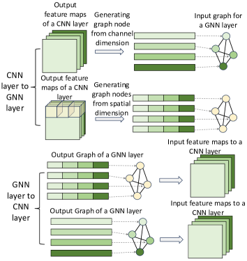
Figure 6: Data Manipulation between CNN and GNN layers

V-C2 Layer fusion for DM layer

To reduce the overhead of the DM layer, the compiler merges the DM layer with the following computation layer (Conv layer or MP layer). This overlaps the data manipulation and the computation. In our hardware design (Figure 5), each PE maintains a Data Manipulation Module (DMM), which pipelines the data manipulation operation and computation.

V-C3 Uniform Mapping

CNN layer (Conv layer) and GNN layer (MP layer) have very different computation patterns. To leverage our flexible hardware design, the compiler performs uniform mapping for the CNN layer and GNN layer in step 2. Both CNN layer and GNN layer are mapped to matrix operations, including matrix multiplication and matrix addition. Since our hardware architecture is optimized for various matrix operations, both the CNN layer and GNN layer can be efficiently executed using our unified architecture design.

V-C4 Data Layout Centric Mapping

CNN layer and GNN layer have very different data layouts. To reduce the data manipulation overhead (Figure 6) between two layers, we proposed to perform data layout centric mapping, which involves the mapping of Conv layers and mapping of MP layers:

Mapping of a Conv layer: As shown in Figure 7, for a Conv layer, the convolution kernel matrix $\mathfrak{W}$ is rearranged into $k_{1}\times k_{2}$ submatrices, denoted as ${\textstyle\{\mathbf{KM}_{i}:0\leqslant i\leqslant k_{1}k_{2}-1\}}$, where each $\mathbf{KM}_{i}$ has dimensions $c_{\text{in}}\times c_{\text{out}}$. The input feature maps $\mathfrak{F}_{\text{in}}$ are organized into a matrix denoted $\mathbf{IFM}$ of size $c_{\text{in}}\times h_{\text{in}}w_{\text{in}}$, with each input feature map represented as a row in this matrix. Each $\mathbf{KM}_{i}$ is multiplied by $\mathbf{IFM}$ to obtain $k_{1}k_{2}$ output matrices, denoted as ${\textstyle\{\mathbf{OFM}_{i}:0\leqslant i\leqslant k_{1}k_{2}-1\}}$, each having dimensions $c_{\text{out}}\times h_{\text{out}}w_{\text{out}}$. Through shift and add (shift-add) operations, the $k_{1}k_{2}$ output matrices are merged into a single output matrix $\mathbf{OFM}$ of size $c_{\text{out}}\times h_{\text{out}}w_{\text{out}}$. $\mathbf{OFM}$ can be further reorganized back to $c_{\text{out}}$ output feature maps. Consequently, a Conv Layer is mapped to matrix multiplication and matrix addition operations.

Data layout of Conv Layer: The proposed mapping strategy brings several benefits: (1) The computation of a Conv Layer is mapped to the matrix operations associated with the computation primitives. (2) The reorganization of data layout for the kernel matrix ($\mathfrak{W}$) occurs at compile time, incurring a one-time cost. (3) The data layout for both $\mathbf{IFM}$ and $\mathbf{OFM}$ remains consistent without the need for data layout transformations between consecutive Conv Layers. (4) Most importantly, the data layout of $\mathbf{IFM}$/$\mathbf{OFM}$ can simplify the data layout manipulation between CNN layer and GNN layer. For example, if the data manipulation layer performs channel-to-node transformation, each row of $\mathbf{IFM}$/$\mathbf{OFM}$ corresponds to a channel in the feature maps of a CNN layer. $\mathbf{IFM}$/$\mathbf{OFM}$ can serves as the input feature matrix for the following MP layer. If the data manipulation layer performs patch-to-node transformation, each column or several columns of $\mathbf{IFM}$/$\mathbf{OFM}$ corresponds to an image patch in the feature maps of a CNN layer. The following MP layer can load node features through matrix transpose, which can be efficiently executed by the Data Manipulation Module.

Figure 7: Mapping a Conv layer to matrix operations

Mapping of MP layer: An MP layer is mapped to the multiplication of graph adjacency matrix $\mathbf{A}$ and feature matrix $\mathbf{H}$. This matrix multiplication will be mapped to either dense computation primitive (DDMM) or sparse computation primitive (SpDMM), which will be introduced later (Section V-C5) in detail. To reduce the overhead of data manipulation from MP layer to Conv layer (Figure 6), the compiler utilizes the Buffer-to-pipeline (B2P) routing network for channel shuffling in DDMM and SpDMM. Because for the data from a GNN layer to a CNN layer (Figure 6), each node feature vector or a piece of node feature vector needs to be routed to the corresponding channel of the feature maps of a CNN layer. During compilation, the compiler assigns a channel index for each node feature vector or a piece of feature vector. During hardware execution, when performing DDMM or SpDMM, the B2P routing network routes the feature vector to the corresponding channel stored in the result buffer. Through this on-the-fly channel shuffling, we eliminate the overhead of data manipulation from the GNN layer to the CNN layer.

V-C5 Sparsity-aware primitive mapping

In step 2, both CNN layers and GNN layers are mapped to matrix operations. Nevertheless, the weight matrix of a CNN/GNN layer or the adjacency matrix of a GNN layer can have different data sparsity. To exploit the data sparsity, the compiler performs sparsity-aware primitive mapping in step 4. In Step 4, for each matrix multiplication operation, the compiler maps it to dense computation primitive (DDMM) and sparse computation primitive (SpDMM) based on the data sparsity and performance models of computation primitives (Section IV-A).

VI Implementation Details

Hardware: We implement the accelerator and the APU (Figure 3) on an Alveo U250 FPGA [44]. We empirically set $p_{\text{ca}}=16$ for each PE and use the half-precision floating-point data format (fp16). The Alveo U250 board consists of four Super Logic Regions (SLRs). Each SLR can be deployed with 2 PEs, except for SLR1, where half of it is occupied by FPGA shell and APU. We utilize Verilog HDL for developing the PE, and use MicroBlaze [38] IP core from AMD Xilinx for implementing the APU. FPGA synthesis and place-route are carried out using Vivado 2022.2. The generated device map and resource utilization are reported in Figure 8. We also perform frequency optimization following the methodology in Xilinx DPU [45] to set the frequency of the computation units ($f_{\text{cu}}=600$ MHz) to double that of the data buffers ($f_{\text{buffer}}=300$ MHz), enhancing the peak performance of the accelerator.

Impact of resource sharing: As discussed in Section IV, different computational primitives share the same set of computation units, on-chip buffers, and routing networks. The wires of different primitives and multiplexers for selecting data paths incur extra area costs. In each PE, these wires and multiplexers consume 37K LUTs (Figure 8), taking 31% LUTs consumption of a PE (A PE consumes 118K LUTs). Through resource sharing, our PE design only costs extra 31% LUTs for supporting various computation primitives.

Compiler: We develop the compiler using Python built upon TVM infrastructure [42]. Based on it, we develop our own intermediate representation, compilation workflow, and compiler optimizations. The compiler takes the computation graph generated by PyTorch [46] and the metadata of input data as input. We develop customized intermediate representation (IR) as TVM prime functions. The five-step compilation is implemented as IR transformation passes to process the generated IR step by step. The output of the compiler is a sequence of instructions that is stored in a binary file.

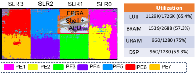
Figure 8: Device map on Alveo U250 FPGA

VII Experimental Results

Overview: We conduct experiments to demonstrate two key aspects: (1) Scope: GCV-Turbo’s versatility to handle a wide range of GNN-based CV tasks as well as traditional CNNs and GNNs; (2) Performance: GCV-Turbo’s ability to achieve high performance, especially for the end-to-end acceleration of GNN-based CV tasks. A comparison of scope and performance are summarized in Table I and Table II, respectively. Table I clearly illustrates that unlike existing CNN DSAs [16, 17, 18, 19, 20, 21, 22] and GNN accelerators [23, 24, 25, 26, 27, 28, 29], which target only one specific scope (either CNNs or GNNs), GCV-Turbo can handle all three scopes – CNNs, GNNs, as well as GNN-based CV. We note that current state-of-the-art implementations of GNN-based CV tasks run these ML models on CPUs or GPUs [47, 48, 49, 50, 51] (given the limited scope of CNN DSAs and GNN accelerators). Thus, a natural performance comparison of GCV-Turbo is with standalone CPUs or GPUs for such tasks. Table II shows a comprehensive comparison of GCV-Turbo versus all alternative baselines - standalone CPU, GPU as well as all the DSAs. Note that GCV-Turbo not only offers comparable performance with CNN DSAs and GNN accelerators within their specialized scopes, it also outperforms CPU and GPU platforms in all three scopes.

Table I: Scope of various accelerators

Scope 1 (CNNs) Scope 2 (GNNs) Scope 3 (GNN-based CV) Performance Comparison CPU and GPU ✓ ✓ ✓ See Section VII-B CNN DSAs [16, 17, 18, 19, 20, 21, 22] ✓ ✗ ✗ See Section VII-D1 GNN Accelerators [23, 24, 25, 26, 27, 28, 29] ✗ ✓ ✗ See Section VII-D2 GCV-Turbo ✓ ✓ ✓

Table II: Average speedup achieved by GCV-Turbo over various baselines within their specialized scopes. Each entry represents the performance of GCV-Turbo divided by the performance of the respective baseline. “Not supported” means that the scope is not supported by the baseline.

CNNs GNNs GNN-based CV tasks CPU (GPU) $418.8\times$ ($1.8\times$) $499.5\times$ ($3.2\times$) $68.4\times$ ($4.1\times$) CNN DSAs $0.88-0.93\times$ Not supported Not supported GNN Accelerators Not supported $1.03\times-1.25\times$ Not supported

The rest of this section is organized as follows: (1) Section VII-A introduces the benchmarks, baselines, metrics, and datasets. (2) Section VII-B presents the comparison results with state-of-the-art CPU and GPU on six GNN-based CV tasks, and standalone CNNs and GNNs. (3) Section VII-C shows the impact of compiler optimizations. (4) Section VII-D compares GCV-Turbo’s performance with that of state-of-the-art CNN and GNN accelerators, within their respective scopes.

VII-A Benchmarks, Baselines, and Metrics

Benchmarks: We collect benchmarks from three scopes, including (1) scope 3 (GNN-based CV): representative GNN-based CV tasks, as elaborated in Table III, which cover diverse data modalities and model types. (2) scope 1 (CNNs): popular CNN models for CV tasks, including c1: AlexNet, c2: ResNet-50 [7], c3: ResNet-101 [7], c4: VGG16 [52], and c5: VGG19 [52]; (3) scope 2 (GNNs): widely used GNN models (g1: GCN [53], g2: GraphSAGE [54], g3: GAT [55]);

Table III: Details of evaluated GNN-based CV tasks

Notation Task Input Modality Model Type Dataset b1 [3] Few-shot image classification image CNN + GNN Omniglot [56] b2 [4] Multi-label image classification image CNN + GNN MS-COCO [57] b3 [5] Image segmentation image CNN + GNN Cityscapes [58] b4 [6] Skeleton-based action recognition human skeleton CNN + GNN NTU RGB+D [59] b5 [31] SAR automatic target classification radar signal CNN + GNN MSTAR [60] b6 [10] Point cloud classification point cloud GNN ModelNet40 [61]

Table IV: Statistics of the graphs in GNN-based CV tasks

Model # of vertices # of edges Feature length Model # of vertices # of edges Feature length b1 25-100 300-5000 300-400 b4 25 75-125 9600-19200 b2 80 6400 300-2048 b5 16384 131072 48 b3 100-300 10000-30000 561-33153 b6 1024 10000-30000 64-1024

Baselines: We compare the performance with the implementations on CPU and GPU as shown in Table V.

Table V: Specifications of platforms

Platforms CPU GPU GCV-Turbo Platform AMD Ryzen 3990x Nvidia RTX A5000 Alveo U250 Platform Technology TSMC 7 nm Samsung 8 nm TSMC 16 nm Frequency 2.90 GHz 1170 MHz 600/300 MHz Peak Performance 3.7 TFLOPS 27.7 TFLOPS 1.08 TFLOPS On-chip Memory 256 MB L3 cache 6 MB L2 cache 45 MB Memory Bandwidth 107 GB/s 768 GB/s 77 GB/s

Performance Metrics: We consider two performance metrics (1) batch-size-one latency: this measures the accelerator’s latency when the batch size is equal to one. In applications like autonomous driving [62], low latency is critical for ensuring safety; (2) throughput: when comparing with state-of-the-art CNN accelerators for standalone CNNs (Section XI), we use throughput as the performance metric. CNN accelerator performance is typically reported in throughput [16, 20].

VII-B Comparison with CPU and GPU Implementations

In this section, we provide a comprehensive comparison between GCV-Turbo and CPU/GPU across the three scopes (Table I). The summarized results can be found in Table II.

VII-B1 Evaluation on Scope 3 (GNN-based CV tasks)

Figure 9 displays the comparison results with CPU and GPU performance on six representative GNN-based CV tasks. The CPU and GPU implementations of these six tasks are from the well-optimized open-source implementations [47, 48, 49, 50, 51], which utilize the optimized CUDA library for CNN and GNN layers. Note that b3 employs two different CNN models, ResNet-50 and ResNet-101, in combination with their proposed GNN layers, resulting in two combinations denoted as b3-r50 and b3-r101, respectively. On average, GCV-Turbo achieves $68.4\times$ and $4.1\times$ latency reduction compared with CPU and GPU, respectively. This speedup is attributed to two factors: (1) The proposed accelerator utilizes unified architecture to accelerate both CNN and GNN layers, improving resource utilization. (2) Our compiler optimizations hide and eliminate the overhead of data layouts transformation between CNN and GNN layers. As illustrated in Figure 9, GCV-Turbo achieves a higher speedup on b1 and b4-6, due to (1) As shown in breakdown analysis below, GNN layers constitute a larger portion of the workload in b1 and b4-6. GCV-Turbo can achieve a higher speedup for the GNN layers due to its optimized architecture for irregular computation in GNN. (2) As shown in Table VI, the model b1 and b4-6 can fit in the on-chip memory of our accelerator. Due to the customized on-chip memory organization, the Computation Array can access the parameters of the model in one clock cycle. In contrast, GPUs have complex cache hierarchy and small L1 cache (128 KB per SM); Accessing the parameters requires navigating through a complex cache hierarchy, resulting in higher latency.

Discussion on the throughput of GPU: While GCV-Turbo achieves lower latency when batch size is 1, GPU can achieve higher throughput by increasing the batch size (e.g., 8/16/32) as GPU has higher peak performance and memory bandwidth. Nevertheless, this work targets latency-sensitive applications (e.g., autonomous driving). For higher throughput, it requires FPGA vendors to develop more powerful FPGA boards with more hardware resources.

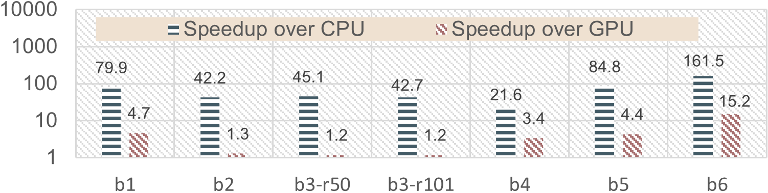
Figure 9: Speedup (latency reduction) over CPU and GPU on GNN-based CV tasks

Table VI: Model size in GNN-based CV tasks

Task b1 b2 b3-r50 b3-r101 b4 b5 b6 Model size (MB) 9.6 115 66 114 5.2 0.76 1.67

Figure 10: Proportion of hardware execution latency of various portions (CNN portion and GNN portion) on GCV-Turbo.

Breakdown Analysis: We conduct a breakdown analysis to understand the speedup of GCV-Turbo compared with the GPU on b1-6. The results, depicted in Figure 2 and 10, demonstrate that different GNN-based CV tasks consist of varying proportions of CNN and GNN layers, and data layout transformation. Table VII presents the breakdown analysis of speedup over the baseline GPU. GCV-Turbo achieves a speedup of $1.2-2.4\times$ on the CNN portion and $1.3-15.2\times$ on the GNN portion for various GNN-based CV tasks. Moreover, through our compiler optimizations, the overhead of data layout transformation is completely reduced and hided, leading to higher latency reduction.

Table VII: Speedup (batch-size-one latency) of GCV-Turbo over GPU on various portions of the GNN-based CV tasks. For layout transformation, the speedup is $\infty$ because GCV-Turbo completely eliminates its overhead.

b1 b2 b3-r50 b3-r101 $\verb|b4|$ b5 b6 CNN layers $2.4\times$ $1.2\times$ $1.2\times$ $1.2\times$ $1.8\times$ $2.3\times$ N/A GNN layers $7.6\times$ $6.8\times$ $1.3\times$ $1.3\times$ $8.4\times$ $6.5\times$ $15.2\times$ Layout transformation $\infty$ $\infty$ $\infty$ $\infty$ $\infty$ $\infty$ $0$ Total $5.1\times$ $1.3\times$ $1.2\times$ $1.2\times$ $3.6\times$ $4.6\times$ $15.2\times$

VII-B2 Evaluation on Scope 1 (CNNs)

Table VIII illustrates the comparison between GCV-Turbo and highly-optimized CPU and GPU implementations [63] across various widely used CNNs. On average, GCV-Turbo achieves $418.8\times$ ($1.8\times$) latency reduction compared with CPU (GPU) implementations.

Table VIII: Speedup (batch-size-one latency) over CPU and GPU on various CNNs

Model c1: AlexNet c2: ResNet50 c3: ResNet101 c4: VGG16 c5: VGG19 Speedup over CPU $182\times$ $43\times$ $42\times$ $971\times$ $855\times$ Speedup over GPU $3.9\times$ $1.2\times$ $1.2\times$ $1.4\times$ $1.5\times$

VII-B3 Evaluation on Scope 2 (GNNs)

We evaluate GCV-Turbo using various GNN models and graph datasets. Table IX displays the speedup achieved by GCV-Turbo over the CPU and GPU platforms. The implementation on CPU and GPU utilizes the state-of-the-art GNN library, PyTorch Geometric [37]. On average, GCV-Turbo achieves a speedup of $499.5\times$ compared with CPU and $3.2\times$ compared with GPU.

Table IX: Speedup over CPU/GPU across various GNNs and graph datasets. [] denotes the speedup of GCV-Turbo over CPU, while () denotes the speedup of GCV-Turbo over GPU.

Cora [53] CiteSeer [53] PubMed [53] Flickr [54] $\verb|g1|$: GCN [$76.2\times$] ($6.7\times$) [$28.8\times$] ($2.7\times$) [$1009\times$] ($2.4\times$) [$312\times$] ($2.4\times$) $\verb|g2|$: SAGE [$131.4\times$] ($2.5\times$) [$119.7\times$] ($1.9\times$) [$178.9\times$] ($2.1\times$) [$421.9\times$] ($3.6\times$) $\verb|g3|$: GAT [$2250\times$] ($6.8\times$) [$1016\times$] ($2.9\times$) [$178.9\times$] ($2.1\times$) [$278.8\times$] ($2.0\times$)

VII-C Impact of Compiler Optimizations

We evaluate the impact of two compiler optimizations:

Layer fusion: Layer fusion yields a speedup ranging from $11.8\%$ to $48.9\%$ across the six GNN-based CV tasks. This speedup can be attributed to layer fusion’s capacity to enhance task-level parallelism, reduce external memory traffic, and decrease the overall computational complexity.

Sparsity-aware mapping: As the weight matrices of the CNN portions in b1-b6 remain unpruned, sparsity-aware mapping does not accelerate the CNN portion. As a result, our speedup measurements exclusively focus on the GNN portion within b1-b6. The sparsity-aware mapping results in speedup percentages of $5.2\%$, $330\%$, $356\%$, $356\%$, $2.3\%$, $2.3\%$, $20.5\%$, and $0\%$ for the GNN portions within b1 to b6, respectively. The GNN within b6 does not experience any speedup because, in b6, the GNN consists of Linear layers, activation layers, and batch normalization layers. The weight matrices within the Linear layers of b6 do not have data sparsity.

VII-D Comparison with State-of-the-art Accelerators

We compare the performance of GCV-Turbo with CNN DSAs [16, 20] on CNN models in Section VII-D1 and with GNN accelerators [25, 41] on GNN models in Section VII-D2. Different accelerators are implemented on different hardware platforms and use different amount of hardware resources. For a fair comparison, we normalize the performance (latency/throughput) by their respective peak performance (FLOPs). For example, normalized throughput is calculated by: ${\textstyle\scalebox{1.0}{\text{Normalized Throughput of [X]}}=\frac{\scalebox{0.7}{\text{Throughput of [X]}}}{\scalebox{0.7}{\text{Peak performance of [X]}}}}$ where [X] can be AMD DPU [16], OPU [20], BoostGCN [25], GraphAGILE [41], or GCV-Turbo.

Table X: Specifications of CNN/GNN accelerators

CNN DSAs GNN Accelerators Platforms AMD DPU [16] OPU1024 [20] BoostGCN [25] GraphAGILE [41] Platform ZCU102 Xilinx XC7K325T Stratix10 GX Alveo U250 Platform Technology N/A 28 nm Intel 14 nm TSMC 16 nm Peak Performance 1.15 TFLOPS 0.2 TFLOPS 0.64 TFLOPS 0.64 TFLOPS On-chip Memory 32.1 MB 2 MB 45 MB 45 MB Memory Bandwidth 19.2 GB/s 12.8 GB/s 77 GB/s 77 GB/s

VII-D1 Comparison with CNN domain-specific accelerators (DSAs)

We compare GCV-Turbo’s performance with state-of-the-art FPGA-based CNN DSAs, AMD DPU [16] and OPU [20] (Table X), on throughput (Table XI). GCV-Turbo’s throughput is computed as $\frac{1}{\text{latency}}$. GCV-Turbo achieves a normalized throughput of $0.88\times$ and $0.93\times$ compared with OPU and DPU on c1-c5. These results demonstrate GCV-Turbo’s competitive throughput in various CNN models, despite slight lower performance. These throughput differences are due to two design trade-offs: GCV-Turbo’s versatility, supporting both CNNs and GNNs, sacrifices some CNN-specific architectural optimizations. For example, OPU’s multi-level parallelism is fine-tuned for CNN convolution operations, whereas GCV-Turbo’s architecture is more generalized. GCV-Turbo’s compilation flow optimizes CNNs and GNNs holistically but cannot support certain convolution-specific optimizations. DPU, for example, selects dataflow for convolutional layers based on kernel size, which cannot be directly applied to GNN layers. Moreover, due to CNN-specific optimizations, OPU and DPU have higher efficiency for using limited DDR memory bandwidth for CNNs. However, OPU and DPU compilers do not support GNNs, and their architectures are inefficient for irregular computations and memory access patterns of GNNs.

Table XI: Comparison of inference throughput (images/second) with CNN DSAs on various CNN models

Throughput (unnormalized) Normalized average speedup of GCV-Turbo over the DSA c1 c2 c3 c4 c5 DPU [16] N/A $43.4$ $38.8$ 274 N/A $0.93\times$ OPU1024 [20] N/A $12.2$ $9.7$ $54.4$ $27$ $0.88\times$ GCV-Turbo $512.9$ 58.8 46.5 $254.7$ 127.3 $1\times$

VII-D2 Comparison with GNN Accelerators

We compare GCV-Turbo with state-of-the-art GNN accelerators, BoostGCN [25], GraphAGILE [41], and FlowGNN [26] (see Table X). Latency measurements follow the methodology from [25, 41], focusing on GCN model and various non-CV graph datasets (Citation networks: CO [53], CI [53], PU [53]; Recommendation systems: FL [64], RE [54], YE [64], AP [64]). Table XII presents the results, where latency is normalized by peak performance of the hardware platform to obtain the speedup. GCV-Turbo outperforms BoostGCN and GraphAGILE with speedups of $1.25\times$ and $1.03\times$, respectively. BoostGCN’s inferior performance is attributed to separate sparse and dense computation hardware modules, leading to underutilization. In contrast, GCV-Turbo optimizes resource usage with a unified architecture for both sparse and dense computations in GNNs. The slight advantage over GraphAGILE is due to GCV-Turbo’s sparsity-aware mapping (Section V-C5), considering data sparsity in the input graph’s connectivity. GCV-Turbo maps computations to DDMM for densely connected subgraphs, unlike GraphAGILE, which neglects data sparsity in graph connectivity. Compared with FlowGNN, GCV-Turbo performs lower because (1) FlowGNN leverages sparsity in graph feature matrices (CO, CI, PU has high data sparsity ($>90\%$) in feature matrices), while GCV-Turbo only uses sparsity in graph adjacency and weight matrices, and (2) FlowGNN generates optimized hardware implementation for different input models. However, the above two optimizations of FlowGNN are unattractive for CV tasks because (1) the sparsity of graph feature matrices is only known during hardware execution; Utilizing its sparsity needs on-the-fly sparsity profiling and data format transformation, causing extra preprocessing overhead. Moreover, the execution time varies with the sparsity of the input data. However, autonomous driving requires deterministic latency for safety. (2) An autonomous driving system will execute various models for various data modalities. Generating optimized bitstreams for each model incurs large latency for switching between the bitstreams through dynamic reconfiguration.

Table XII: Comparison of hardware execution latency (ms) with state-of-the-art GNN accelerators

Latency (ms) (unnormalized) Normalized average speedup of GCV-Turbo over the accelerator CO CI PU FL RE YE AP BoostGCN N/A N/A N/A $20.1$ $98.5$ $193.5$ $793.5$ $1.25\times$ GraphAGILE $0.819$ $2.55$ $2.24$ $11.5$ $97.2$ $104.3$ $315$ $1.03\times$ FlowGNN $6.9E-3$ $8.3E-3$ $53E-3$ $N/A$ $136$ $N/A$ $N/A$ $0.003\times$ (CO/CI/PU), $0.38\times$ (RE) GCV-Turbo $0.48$ $1.47$ $1.25$ $6.09$ $72.7$ $43.5$ $196.9$ $1\times$

VIII Conclusion and Future Work

We introduced GCV-Turbo, the first domain-specific accelerator for GNN-based CV. It bridges the gap between state-of-the-art CNN DSAs and GNN accelerators, leading to end-to-end acceleration of GNN-based CV. GCV-Turbo can also handle standalone CNNs and GNNs as effectively as specialized accelerators while optimizing the execution of CNN and GNN layers within GNN-based CV tasks. With its unified architecture and compilation workflow, GCV-Turbo achieved average latency reduction of $68.4\times$ and $4.1\times$ compared with state-of-the-art CPU and GPU implementations. In the future, we plan to broaden GCV-Turbo’s capabilities to accommodate Vision Transformer (ViT) models.

References

- [1] C. Chen, Y. Wu, Q. Dai, H.-Y. Zhou, M. Xu, S. Yang, X. Han, and Y. Yu, “A survey on graph neural networks and graph transformers in computer vision: A task-oriented perspective,” arXiv preprint arXiv:2209.13232, 2022.
- [2] S. H. Chowdhury, M. R. Sany, M. H. Ahamed, S. K. Das, F. R. Badal, P. Das, Z. Tasneem, M. M. Hasan, M. R. Islam, M. F. Ali et al., “A state-of-the-art computer vision adopting non-euclidean deep-learning models,” International Journal of Intelligent Systems, vol. 2023, 2023.
- [3] V. Garcia and J. Bruna, “Few-shot learning with graph neural networks,” in 6th International Conference on Learning Representations, ICLR 2018, 2018.
- [4] Z.-M. Chen, X.-S. Wei, P. Wang, and Y. Guo, “Multi-label image recognition with graph convolutional networks,” in Proceedings of the IEEE/CVF conference on computer vision and pattern recognition, 2019, pp. 5177–5186.
- [5] L. Zhang, X. Li, A. Arnab, K. Yang, Y. Tong, and P. Torr, “Dual graph convolutional network for semantic segmentation,” in Proceedings of the British Machine Vision Conference 2019. British Machine Vision Association, 2019.
- [6] S. Yan, Y. Xiong, and D. Lin, “Spatial temporal graph convolutional networks for skeleton-based action recognition,” in Proceedings of the AAAI conference on artificial intelligence, vol. 32, no. 1, 2018.
- [7] K. He, X. Zhang, S. Ren, and J. Sun, “Deep residual learning for image recognition,” in Proceedings of the IEEE conference on computer vision and pattern recognition, 2016, pp. 770–778.
- [8] A. Dosovitskiy, L. Beyer, A. Kolesnikov, D. Weissenborn, X. Zhai, T. Unterthiner, M. Dehghani, M. Minderer, G. Heigold, S. Gelly et al., “An image is worth 16x16 words: Transformers for image recognition at scale,” in ICLR.
- [9] W. Shi and R. Rajkumar, “Point-gnn: Graph neural network for 3d object detection in a point cloud,” in Proceedings of the IEEE/CVF conference on computer vision and pattern recognition, 2020, pp. 1711–1719.
- [10] C. R. Qi, H. Su, K. Mo, and L. J. Guibas, “Pointnet: Deep learning on point sets for 3d classification and segmentation,” in Proceedings of the IEEE conference on computer vision and pattern recognition, 2017, pp. 652–660.
- [11] C. R. Qi, L. Yi, H. Su, and L. J. Guibas, “Pointnet++: Deep hierarchical feature learning on point sets in a metric space,” Advances in neural information processing systems, vol. 30, 2017.
- [12] T. Wen, J. Zhuang, Y. Du, L. Yang, and J. Xu, “Dual-sampling attention pooling for graph neural networks on 3d mesh,” Computer Methods and Programs in Biomedicine, vol. 208, p. 106250, 2021.
- [13] W. Tang, Y. Gong, and G. Qiu, “Feature preserving 3d mesh denoising with a dense local graph neural network,” Computer Vision and Image Understanding, vol. 233, p. 103710, 2023.
- [14] J. Redmon, S. Divvala, R. Girshick, and A. Farhadi, “You only look once: Unified, real-time object detection,” in Proceedings of the IEEE conference on computer vision and pattern recognition, 2016, pp. 779–788.
- [15] J. Wu, L. Wang, L. Wang, J. Guo, and G. Wu, “Learning actor relation graphs for group activity recognition,” in Proceedings of the IEEE/CVF Conference on computer vision and pattern recognition, 2019, pp. 9964–9974.
- [16] “Dpu.” [Online]. Available: https://www.xilinx.com/products/intellectual-property/dpu.html
- [17] E. Qin, A. Samajdar, H. Kwon, V. Nadella, S. Srinivasan, D. Das, B. Kaul, and T. Krishna, “Sigma: A sparse and irregular gemm accelerator with flexible interconnects for dnn training,” in 2020 IEEE International Symposium on High Performance Computer Architecture (HPCA), 2020, pp. 58–70.
- [18] N. Jouppi, C. Young, N. Patil, and D. Patterson, “Motivation for and evaluation of the first tensor processing unit,” ieee Micro, vol. 38, no. 3, pp. 10–19, 2018.
- [19] M. S. Abdelfattah, D. Han, A. Bitar, R. DiCecco, S. O’Connell, N. Shanker, J. Chu, I. Prins, J. Fender, A. C. Ling et al., “Dla: Compiler and fpga overlay for neural network inference acceleration,” in FPL. IEEE, 2018.
- [20] Y. Yu, C. Wu, T. Zhao, K. Wang, and L. He, “Opu: An fpga-based overlay processor for convolutional neural networks,” IEEE Transactions on Very Large Scale Integration (VLSI) Systems, vol. 28, no. 1, pp. 35–47, 2019.
- [21] Y. Chen, T. Luo, S. Liu, S. Zhang, L. He, J. Wang, L. Li, T. Chen, Z. Xu, N. Sun et al., “Dadiannao: A machine-learning supercomputer,” in 2014 47th Annual IEEE/ACM International Symposium on Microarchitecture. IEEE, 2014, pp. 609–622.
- [22] T. Luo, S. Liu, L. Li, Y. Wang, S. Zhang, T. Chen, Z. Xu, O. Temam, and Y. Chen, “Dadiannao: A neural network supercomputer,” IEEE Transactions on Computers, vol. 66, no. 1, pp. 73–88, 2017.
- [23] M. Yan and L. Deng, “Hygcn: A gcn accelerator with hybrid architecture,” in 2020 IEEE International Symposium on High Performance Computer Architecture (HPCA). IEEE, 2020.
- [24] T. Geng, A. Li, R. Shi, C. Wu, T. Wang, Y. Li, P. Haghi, A. Tumeo, S. Che, S. Reinhardt et al., “Awb-gcn: A graph convolutional network accelerator with runtime workload rebalancing,” in 2020 53rd Annual IEEE/ACM International Symposium on Microarchitecture (MICRO). IEEE, 2020, pp. 922–936.
- [25] B. Zhang, R. Kannan, and V. Prasanna, “Boostgcn: A framework for optimizing gcn inference on fpga,” in 2021 IEEE 29th Annual International Symposium on Field-Programmable Custom Computing Machines (FCCM). IEEE, 2021, pp. 29–39.
- [26] R. Sarkar, S. Abi-Karam, Y. He, L. Sathidevi, and C. Hao, “Flowgnn: A dataflow architecture for real-time workload-agnostic graph neural network inference,” in 2023 IEEE International Symposium on High-Performance Computer Architecture (HPCA). IEEE, 2023, pp. 1099–1112.
- [27] S. Liang, C. Liu, Y. Wang, H. Li, and X. Li, “Deepburning-gl: an automated framework for generating graph neural network accelerators,” in Proceedings of the 39th International Conference on Computer-Aided Design, 2020, pp. 1–9.
- [28] B. Zhang, H. Zeng, and V. Prasanna, “Hardware acceleration of large scale gcn inference,” in 2020 IEEE 31st International Conference on Application-specific Systems, Architectures and Processors (ASAP). IEEE, 2020, pp. 61–68.
- [29] T. Geng, C. Wu, Y. Zhang, C. Tan, C. Xie, H. You, M. Herbordt, Y. Lin, and A. Li, “I-gcn: A graph convolutional network accelerator with runtime locality enhancement through islandization,” in MICRO-54: 54th annual IEEE/ACM international symposium on microarchitecture, 2021, pp. 1051–1063.
- [30] J. Li, A. Louri, A. Karanth, and R. Bunescu, “Gcnax: A flexible and energy-efficient accelerator for graph convolutional neural networks,” in 2021 IEEE International Symposium on High-Performance Computer Architecture (HPCA). IEEE, 2021, pp. 775–788.
- [31] B. Zhang, S. Wijeratne, R. Kannan, V. Prasanna, and C. Busart, “Graph neural network based sar automatic target recognition with human-in-the-loop,” in Algorithms for Synthetic Aperture Radar Imagery XXX, vol. 12520. SPIE, 2023, pp. 196–198.
- [32] B. Zhang, H. Zeng, and V. Prasanna, “Graphagile: An fpga-based overlay accelerator for low-latency gnn inference,” IEEE Transactions on Parallel and Distributed Systems, 2023.
- [33] D. Wen, J. Jiang, J. Xu, K. Wang, T. Xiao, Y. Zhao, and Y. Dou, “Rfc-hypgcn: A runtime sparse feature compress accelerator for skeleton-based gcns action recognition model with hybrid pruning,” in 2021 IEEE 32nd International Conference on Application-specific Systems, Architectures and Processors (ASAP). IEEE, 2021, pp. 33–40.
- [34] L. Shi, Y. Zhang, J. Cheng, and H. Lu, “Two-stream adaptive graph convolutional networks for skeleton-based action recognition,” in Proceedings of the IEEE/CVF conference on computer vision and pattern recognition, 2019, pp. 12 026–12 035.
- [35] Y. Lin, Z. Zhang, H. Tang, H. Wang, and S. Han, “Pointacc: Efficient point cloud accelerator,” in MICRO-54: 54th Annual IEEE/ACM International Symposium on Microarchitecture, 2021, pp. 449–461.
- [36] A. Lerer, L. Wu, J. Shen, T. Lacroix, L. Wehrstedt, A. Bose, and A. Peysakhovich, “Pytorch-biggraph: A large-scale graph embedding system,” arXiv preprint arXiv:1903.12287, 2019.
- [37] M. Fey and J. E. Lenssen, “Fast graph representation learning with PyTorch Geometric,” in ICLR Workshop on Representation Learning on Graphs and Manifolds, 2019.
- [38] “Microblaze.” [Online]. Available: https://docs.xilinx.com/v/u/2021.1-English/ug984-vivado-microblaze-ref
- [39] S. Zhou, R. Kannan, V. K. Prasanna, G. Seetharaman, and Q. Wu, “Hitgraph: High-throughput graph processing framework on fpga,” IEEE Transactions on Parallel and Distributed Systems, 2019.
- [40] X. Chen, H. Tan, Y. Chen, B. He, W.-F. Wong, and D. Chen, “Thundergp: Hls-based graph processing framework on fpgas,” in The 2021 ACM/SIGDA International Symposium on Field-Programmable Gate Arrays, 2021, pp. 69–80.
- [41] B. Zhang, H. Zeng, and V. K. Prasanna, “Graphagile: An fpga-based overlay accelerator for low-latency gnn inference,” IEEE Transactions on Parallel and Distributed Systems, vol. 34, no. 9, pp. 2580–2597, 2023.
- [42] T. Chen, T. Moreau, Z. Jiang, L. Zheng, E. Yan, H. Shen, M. Cowan, L. Wang, Y. Hu, L. Ceze et al., “TVM: An automated End-to-End optimizing compiler for deep learning,” in 13th USENIX Symposium on Operating Systems Design and Implementation (OSDI 18), 2018, pp. 578–594.
- [43] B. Barney et al., “Introduction to parallel computing,” Lawrence Livermore National Laboratory, vol. 6, no. 13, p. 10, 2010.
- [44] “Xilinx alveo u250.” [Online]. Available: https://docs.xilinx.com/r/en-US/ds962-u200-u250/FPGA-Resource-Information
- [45] “Frequency optimization.” [Online]. Available: https://docs.xilinx.com/r/en-US/ds962-u200-u250/FPGA-Resource-Information
- [46] A. Paszke, S. Gross, F. Massa, A. Lerer, J. Bradbury, G. Chanan, T. Killeen, Z. Lin, N. Gimelshein, L. Antiga et al., “Pytorch: An imperative style, high-performance deep learning library,” Advances in neural information processing systems, vol. 32, 2019.
- [47] “Cpu and gpu implementation of few-shot image classification.” [Online]. Available: https://github.com/vgsatorras/few-shot-gnn
- [48] “Cpu and gpu implementation of multi-label image classification.” [Online]. Available: https://github.com/megvii-research/ML-GCN
- [49] “Cpu and gpu implementation of image segmentation.” [Online]. Available: https://github.com/lxtGH/GALD-DGCNet
- [50] “Cpu and gpu implementation of skeleton-based action recognition.” [Online]. Available: https://github.com/yysijie/st-gcn
- [51] “Cpu and gpu implementation of point cloud classification.” [Online]. Available: https://github.com/WeijingShi/Point-GNN
- [52] K. Simonyan and A. Zisserman, “Very deep convolutional networks for large-scale image recognition,” in 3rd International Conference on Learning Representations (ICLR 2015). Computational and Biological Learning Society, 2015.
- [53] T. N. Kipf and M. Welling, “Semi-supervised classification with graph convolutional networks,” in International Conference on Learning Representations, 2016.
- [54] W. Hamilton, Z. Ying, and J. Leskovec, “Inductive representation learning on large graphs,” Advances in neural information processing systems, vol. 30, 2017.
- [55] P. Veličković, G. Cucurull, A. Casanova, A. Romero, P. Liò, and Y. Bengio, “Graph attention networks,” in International Conference on Learning Representations, 2018.
- [56] B. M. Lake, R. Salakhutdinov, and J. B. Tenenbaum, “The omniglot challenge: a 3-year progress report,” Current Opinion in Behavioral Sciences, vol. 29, pp. 97–104, 2019.
- [57] T.-Y. Lin, M. Maire, S. Belongie, J. Hays, P. Perona, D. Ramanan, P. Dollár, and C. L. Zitnick, “Microsoft coco: Common objects in context,” in Computer Vision–ECCV 2014: 13th European Conference, Zurich, Switzerland, September 6-12, 2014, Proceedings, Part V 13. Springer, 2014, pp. 740–755.
- [58] M. Cordts, M. Omran, S. Ramos, T. Rehfeld, M. Enzweiler, R. Benenson, U. Franke, S. Roth, and B. Schiele, “The cityscapes dataset for semantic urban scene understanding,” in Proceedings of the IEEE conference on computer vision and pattern recognition, 2016, pp. 3213–3223.
- [59] J. Liu, A. Shahroudy, M. Perez, G. Wang, L.-Y. Duan, and A. C. Kot, “Ntu rgb+d 120: A large-scale benchmark for 3d human activity understanding,” IEEE Transactions on Pattern Analysis and Machine Intelligence, vol. 42, no. 10, pp. 2684–2701, 2020.
- [60] “Mstar.” [Online]. Available: https://www.sdms.afrl.af.mil/index.php?collection=mstar
- [61] Z. Wu, S. Song, A. Khosla, F. Yu, L. Zhang, X. Tang, and J. Xiao, “3d shapenets: A deep representation for volumetric shapes,” in Proceedings of the IEEE conference on computer vision and pattern recognition, 2015, pp. 1912–1920.
- [62] K. Roszyk, M. R. Nowicki, and P. Skrzypczyński, “Adopting the yolov4 architecture for low-latency multispectral pedestrian detection in autonomous driving,” Sensors, vol. 22, no. 3, p. 1082, 2022.
- [63] “Optimized pytorch implementations for cnn models.” [Online]. Available: https://pytorch.org/vision/stable/models.html
- [64] H. Zeng, H. Zhou, A. Srivastava, R. Kannan, and V. Prasanna, “GraphSAINT: Graph sampling based inductive learning method,” in International Conference on Learning Representations.