BAMBOO: a predictive and transferable machine learning force field framework for liquid electrolyte development

Abstract

Despite the widespread applications of machine learning force field (MLFF) on solids and small molecules, there is a notable gap in applying MLFF to complex liquid electrolytes. In this work, we introduce BAMBOO (ByteDance AI Molecular Simulation Booster), a novel framework for molecular dynamics (MD) simulations, with a demonstration of its capabilities in the context of liquid electrolytes for lithium batteries. We design a physics-inspired graph equivariant transformer architecture as the backbone of BAMBOO to learn from quantum mechanical simulations. Additionally, we pioneer an ensemble knowledge distillation approach and apply it on MLFFs to improve the stability of MD simulations. Finally, we propose the density alignment algorithm to align BAMBOO with experimental measurements. BAMBOO demonstrates state-of-the-art accuracy in predicting key electrolyte properties such as density, viscosity, and ionic conductivity across various solvents and salt combinations. Our current model, trained on more than 15 chemical species, achieves the average density error of 0.01 g/cm³ on various compositions compared with experimental data. Moreover, our model demonstrates transferability to molecules not included in the quantum mechanical dataset. We envision this work as paving the way to a “universal MLFF” capable of simulating properties of common organic liquids.

1 Introduction

Liquid electrolyte is an indispensable component in most of electrochemical energy devices that include, but not limited to lithium ion and lithium metal batteries [1, 2, 3]. The existing commercial electrolytes are primarily carbonate-based, and it is common to find a commercial electrolyte composed of more than five, even up to ten different components to meet various aspects of cell performances. Recent developments have expanded the electrolyte designs to high-concentrated [4], localized high-concentrated [5], and fluorinated ether-based electrolytes [6, 7]. These novel designs aim to engineer molecular-level solvation structures for improved solvation/desolvation [8] performance, solid electrolyte interphase [9], and electrochemical stability [10]. Experimentally exploring molecular interactions for rational design is costly, time-consuming, and heavily reliant on chemists’ intuition and experience. These limitations pose challenges in transitioning from proof of concept in a lab to commercialization, particularly due to the exponential complexity involved in optimizing properties and local solvation structures for multi-component liquid electrolyte systems.

Atomistic simulations offer an efficient and flexible alternative to exhaust experimentation. They can accurately capture the evolving ion-solvent polarizable interactions, thereby, providing reliable bulk and molecular level property predictions. However, requirements such as sufficient simulation time and scale need to be met. Quantum mechanical simulations offer high accuracy in describing electronic properties, yet they are computationally intensive and impractical for studying large-scale and complex systems, such as liquid electrolytes. On the other hand, classical force fields, while computationally efficient, often sacrifice accuracy in capturing the intricate solvation structures and dynamic behavior of electrolytes. Hence, there exists a pressing need for a balanced and general approach that can reconcile the trade-off between accuracy, speed, and complexity in modeling liquid electrolytes with different molecular solvents and varying salt concentrations.

In recent years, there has been a growing utilization of machine learning force fields (MLFFs) [11] to perform molecular dynamics (MD) simulations [12]. This trend is primarily attributed to MLFFs’ ability to deliver results significantly faster than $ab$-$initio$ quantum mechanical simulations, while also offering more degree of freedom to fit quantum mechanical data compared with classical force fields [13]. Consequently, MLFFs have demonstrated ability for enhanced accuracy in predicting forces compared with classical force fields when benchmarked against quantum mechanics.

The development of MLFFs has seen two prominent trends. On one hand, there has been a gradual integration of novel concepts from the field of machine learning into MLFF design. This evolution has seen a shift from local descriptor-based, rotation-invariant MLFFs [14, 15, 16] towards graph neural network (GNN)-based models [17] and rotation-equivariant MLFFs [18] employing the transformer architecture [19, 20]. On the other hand, there has been an emphasis on incorporating interactions grounded in clear physical foundation into MLFFs. These include electrostatic [21, 22], dispersion [23, 24], and spin-spin interactions [25, 26].

With advancements in the model architecture of MLFFs, the concept of “universal machine learning force field”, which aims to employ a single MLFF to simulate a wide range of systems, has garnered increasing attention within the realms of solid-state materials [27, 28, 29, 30, 31] and bio-organic molecules [23, 32]. However, when it comes to liquids, particularly liquid electrolytes containing solvents and ions, a universal MLFF that can accurately predict multiple properties across various solvents and salts is still lacking. This limitation may arise from the complex local structures inherent in liquid electrolytes, such as the coexistence of different structural motifs like solvent-separated ion pairs (SSIP), contacted ion pairs (CIP), and aggregates (AGG). As a result, despite some studies utilizing MLFFs to investigate aqueous systems [33, 34], molecular liquids [35], and ionic liquids [36], there remains a notable scarcity of research specifically focused on MLFFs for liquid electrolytes.

To the best of our knowledge, only two notable previous attempts have been made to simulate liquid electrolytes using MLFFs: Wang $et$ $al.$ [37] utilized Deep Potential [15] to calculate the density and solvation structure of LiFSI in triglyme, and Dajnowicz $et$ $al.$ [38] employed charge-recursive neural network (QRNN) [39] to compute the density, viscosity, and diffusivity of LiPF₆ in carbonate solvents. Despite achieving some success, these studies lack conclusive evidence regarding the generalizability of their findings across a wide range of liquid electrolytes. For instance, Ref. [38] shows that QRNN struggled to achieve high accuracy across both linear and cyclic carbonates simultaneously, as well as solutions with low and high concentrations of LiPF₆.

In addition to the scarcity of studies on MLFFs for liquid electrolytes, there are two overarching challenges associated with MLFFs. As highlighted by Fu $et$ $al.$ [40], MD simulations employing MLFFs often encounter issues of qualitative and quantitative instability, stemming from the inherent randomness in machine learning [41], which limits the practical utility of MLFFs. Moreover, current deep learning-based MLFFs solely rely on learning from quantum mechanical simulations, which do not necessarily guarantee accurate reproduction of experimental measurements across diverse atomistic systems. Although the concept of differentiable molecular simulation [42, 43] has been introduced to optimize classical force fields based on experimentally measured macroscopic observables, to the best of our knowledge, there is currently no deep learning-based MLFF of which parameters are directly optimized using experimental results. One underlying reason for this absence could be that current optimization methods based on differentiable molecular simulations rely on backpropagating the gradients of MD trajectories to train the parameters. This process is computationally expensive and has the possibility to induce overfitting of deep neural network-based MLFFs to the limited amount of experimental data available.

In this work, we introduce the BAMBOO (ByteDance AI Molecular Simulation Booster) workflow, specifically designed for constructing MLFFs for MD simulations of organic liquids, with a particular emphasis on liquid electrolytes. The main methodological contributions of this paper are summarized as follows:

• We propose a novel MLFF model that integrates a graph equivariant transformer (GET) architecture with physics-based division of semi-local, electrostatic and dispersion interactions. Our model demonstrates remarkable generalizability in learning various types of molecules and salts using a single model, and it exhibits transferability to unseen liquid systems.

• We introduce the application of the ensemble knowledge distillation algorithm to enhance the stability of MLFF concerning both qualitative observations and quantitative results obtained from MD simulations.

• We propose a novel physics-inspired density alignment algorithm aiming at aligning MLFF-based MD simulations with experimental data. This innovative approach requires only a minimal amount of experimental data and demonstrates exceptional transferability to liquids not initially included in the alignment process.

As a result, BAMBOO achieves state-of-the-art accuracy in predicting the density, viscosity, and ionic conductivity of various solvents and liquid electrolytes. BAMBOO also demonstrates the capability to discern different atomic partial charges based on molecular local environment, a crucial aspect for accurately describing solvation structures. Finally, BAMBOO shows robust generalizability and transferability to unseen molecules, making it a valuable tool for novel electrolyte designs driven by molecular structure engineering.

2 Results

2.1 Training of BAMBOO

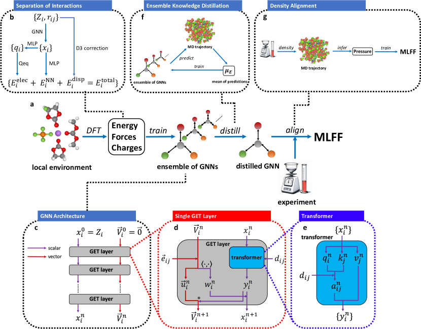
Figure 1: Overview of BAMBOO. a. Schematic of the training process of BAMBOO. b. Separation of interactions in BAMBOO. c, d, e. Schematic of the GNN, the GET layer inside the GNN, and the transformer inside the GET layer, respectively. f, g. Schematic of the ensemble knowledge distillation and density alignment of BAMBOO, respectively.

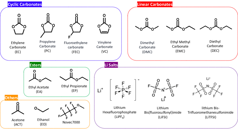
Figure S1: Schematic of the species included in the DFT dataset.

We illustrate the workflow of BAMBOO in Figure 1a. Initially, we sample local atomic environments within liquid electrolytes as gas-phase clusters and subsequently employ DFT to compute their energies, atomic forces, and charges. In our study, aimed at showcasing the broad applicability of BAMBOO, we include diverse molecules and salts in the DFT dataset, as illustrated in Figure S1 in the Supplementary Information. Notably, our focus encompasses components commonly found in liquid electrolytes utilized in Li-ion batteries, such as cyclic carbonates, linear carbonates, as well as Li⁺ cations, and PF${}_{6}^{-}$, bis(fluorosulfonyl)imide (FSI^-), and bis(trifluoromethanesulfonyl)imide (TFSI^-) anions. Additionally, we incorporate two frequently used organic liquids, ethanol (EO) and acetone (ACT), along with an engineering fluid Novec7000 [44] to showcase the generalizability of the trained model. Subsequently, the quantities calculated by DFT are employed to train a group of Graph Neural Networks (GNNs) with different random seeds. To enhance stability in MD simulations, these independently trained GNNs are fused into a single unified GNN via ensemble knowledge distillation [45]. Finally, we employ experimentally measured data, specifically density in this context, to align the MLFF model with experimental observations. Further elaboration on the DFT dataset, training methodology, ensemble knowledge distillation, and density alignment procedures can be found in the subsequent sections and in the Supplementary Information.

In Figure 1b, we delineate the separation of semi-local, electrostatic, and dispersion interactions in BAMBOO. Given the significance of long-range electrostatic and dispersion interactions in simulating liquid electrolytes [46, 47], we explicitly compute their corresponding energies in BAMBOO. Our model takes as input the types of atoms $\{Z_{i}\}$ and the 3D coordinates of atoms $\{r_{i}\}$, which are constructed as follows:

• Semi-local energy is modeled by a GNN comprising graph equivariant transformer (GET) layers whose detailed structure will be introduced in the following subsection. The GET layers take the atom types $\{Z_{i}\}$ and the relative coordinates $\{\vec{r}_{ij}=\vec{r}_{i}-\vec{r}_{j}\}$ of edges $(i,j)$, and output atom representations $\{x_{i}\}$ which captures local environments of each atom. We further input $\{x_{i}\}$ into a multi-layer perceptron (MLP) to obtain the neural network predicted energy $\{E_{i}^{\text{NN}}\}$.

• Electrostatic energy is computed as follows. The atom representations $\{x_{i}\}$ are fed into another MLP to predict the atomic partial charge $\{q_{i}\}$. We then compute electrostatic energy $\{E_{i}^{\text{elec}}\}$ based on the predicted partial charge under the framework of charge equilibrium [48].

• Dispersion energy $\{E_{i}^{\text{disp}}\}$ is directly computed based on the DFT-D3(CSO) correction [49].

Finally, the total atomic energy ${E_{i}^{\text{total}}}$ is obtained by summing ${E_{i}^{\text{NN}}}$, ${E_{i}^{\text{elec}}}$, and ${E_{i}^{\text{disp}}}$, and the total energy of the system $E$ is computed by summing all atomic energies. Further details of the energy model are provided in the Supplementary Information A.2. Regarding forces, as energy is computed based on relative coordinates $\vec{r}_{ij}$, rather than absolute coordinates $\vec{r}_{i}$, the pairwise force can be naturally defined and computed as $\vec{f}_{ij}=\frac{1}{2}(-\frac{\partial E}{\partial r_{ij}}+\frac{\partial E}{\partial r_{ji}})$, satisfying Newton’s Third Law ($\vec{f}_{ij}=-\vec{f}_{ji}$) for computing microscopic stress [50]. The atomic force is then computed by summing the pairwise forces: $\vec{f}_{i}=\sum_{j\neq i}\vec{f}_{ji}$.

2.2 Architecture of GET Layers

In Figure 1c, d, and e, we present the the Graph Equivariant Transformer (GET) architecture utilized in BAMBOO, which draws inspiration mainly from the architecture of TorchMD-Net [20]. Beginning with the atom types $\{Z_{i}\}$ and the relative coordinate vectors between atoms $\{\vec{r}_{ij}\}$, we first initialize the atom scalar representation $x_{i}^{0}$ and the atom vector representation $\vec{V}_{i}^{0}$, as well as the edge scalar representation $d_{ij}$ and the edge vector representation $\vec{e}_{ij}$. Subsequently, we feed $x_{i}^{0}$ and $\vec{V}_{i}^{0}$ into the GET layers to update them iteratively (Figure 1c). As depicted in Figure 1d, within each GET layer, scalar representation $x_{i}^{n}$ undergoes a transformer layer to exchange information with its neighbors within a specified cutoff radius (5Å in this study). Figure 1e illustrates the transformer block designed as attention mechanism [51] on edges. Following the transformer block, on the scalar side, we obtain the intermediate atom scalar representation $y_{i}^{n}$. On the vector side, along with $\vec{e}_{ij}$, the atom vector representation $\vec{V}_{i}^{n}$ is transformed into an intermediate vector representation $\vec{u}_{ij}^{n}$ and another scalar representation $w_{i}^{n}$. Here, the transformation from vector to scalar is achieved through the inner product operation to maintain rotational invariance. Finally, we combine $y_{i}^{n}$ and $w_{i}^{n}$ to obtain the next-layer atom scalar representation $x_{i}^{n+1}$, and combine $y_{i}^{n}$, $\vec{u}_{ij}^{n}$, and $\vec{V}_{i}^{n}$ to obtain the next-layer atom vector representation $\vec{V}_{i}^{n+1}$. In this process, scalar $y_{i}^{n}$ is multiplied to a vector to preserve the equivariance of the vector representation. Analogously, within each GET layer, all neighboring atoms exchange information with one another through the transformer, and scalar and vector representations also exchange information with each other. Detailed equations of the GET architecture are provided in the Supplementary Information A.1. Compared with TorchMD-Net [20], our method enhances efficiency through two key strategies. On one hand, we utilize attention mechanisms on graphs as opposed to global attention, effectively lowering the computational complexity from $\mathcal{O}(N^{2})$ to $\mathcal{O}(N)$. On the other hand, we eliminate certain residual connections that do not significantly contribute to increasing the model’s capacity but instead decelerate it. As a result, our model benefits from a noticeable speed enhancement, as illustrated in Figure 2g and h.

In Figure 2a, b, and c, we elucidate the roles of equivariant features and transformer, as well as partial charge prediction by ablation studies. For predicting energy and forces from DFT, GET demonstrates superior performance compared with the Graph Equivariant Network (GE) and the Graph Invariant Transformer (GIT). Notably, GE lacks a transformer layer, while GIT does not incorporate equivariance features. This comparison highlights the crucial role of both equivariant features and the transformer within GET, as evidenced by the smaller errors observed. Furthermore, we observe that equivariance may hold greater importance than the transformer, as GE demonstrates smaller errors than GIT, suggesting avenues for accelerating inference in future applications. In addition, we conduct a comparison with a model termed GET-no-charge, which excludes the prediction of partial charges. Interestingly, we observed that GET-no-charge outperforms GET in terms of force errors, but it suffers notably larger errors in energy due to the long-range dependence of electrostatic energy (proportional to $1/r$) and the reduced capacity of GNN to capture long-range interactions as opposed to the short-range [52]. As illustrated in Figure 2c, GET exhibits the smallest error in density from MD simulations compared with GE, GIT, and GET-no-charge, likely attributable to its superior performance in predicting DFT quantities overall. These findings collectively emphasize the suitability of the GET architecture in BAMBOO for simulating liquid electrolytes compared with previous MLFFs without equivariance, transformer, and explicit computation of electrostatic interactions. Further results of the ablation study, along with details of the ablated models, are provided in the Supplementary Information D.

In this work, we use LAMMPS [53] as the engine to run MD simulations, and we design the interface between BAMBOO and LAMMPS with inspiration from Allegro [54]. As shown in Table 1 and Figure 2g and h, relative to other GNN-based MLFFs like VisNet [55], Allegro [54], MACE [56] or TorchMD-Net 2.0 [57], BAMBOO achieves a higher inference speed (2 million steps per day for a system with 10,000 atoms on a single NVIDIA A100 GPU). The inference of BAMBOO can be further accelerated by using multiple GPUs in parallel, which will be introduced in a future release.

Table 1: Comparison of the inference speed of BAMBOO with other GNN MLFFs on a gas-phase single molecule 3-(bezyloxy)pyridin-2-amine (3BPA), focusing on a fair comparison. BAMBOO is compared with other MLFFs with spherical harmonic order $L=1$, as BAMBOO exclusively utilizes scalar and vector embeddings. The experiments are conducted on a NVIDIA A100 GPU.

Model	MACE (L=1) [56]	Allegro (L=1) [54]	VisNet (L=1) [55]	BAMBOO
Speed [ms]	17.5	13.0	12.2	6.9

2.3 Ensemble Knowledge Distillation and Density Alignment

Figure 2: Effects of GET layers, ensemble knowledge distillation, and density alignment. a, b, c. Effects of equivariant features, transformer, and charge in BAMBOO. All models are trained using the same DFT training set, excluding ensemble knowledge distillation and density alignment, and their performance is evaluated on the same validation set, comprising energy and forces from DFT and density from experiments. The evaluation metrics include RMSE (root mean squared error) and MAE (mean absolute error) d. Effect of ensemble knowledge distillation on reducing the standard deviation of density from MD simulations by different randomly trained MLFFs. Per-liquid standard deviations are provided in Figure S5. e, f. Effect of density alignment on predictions of density, viscosity, and ionic conductivity from MD. The mean absolute deviation (MAD) is used as a metric, expressed in percentage. Per-liquid density mean absolute error (MAE), as well as viscosity and conductivity MAD, are illustrated in Figure S8. g, h. The inference speed comparison between BAMBOO and TorchMD-Net 2.0 [57]. We compare the 3-layer BAMBOO with the 2-layer TensorNet [58] module implemented in TorchMD-Net 2.0 [57]. We delineate the inference speed in million steps per day in g and in atom times step per millisecond in h. Speeds are tested on a single NVIDIA A100 GPU.

Table 2: Comparison of BAMBOO with other public reports on calculating density, viscosity, and ionic conductivity of liquid electrolytes. The reported error of BAMBOO is from a single model. The reported average error of other studies are from all the available tables and figures in the references.

Model	System(s)	Density error (g/cm3)	Viscosity error (%)	Conductivity error (%)
BAMBOO	12 molecules, 3 salts	0.011	17.1	26.3
DP[15, 37]	1 molecule,1 salt	0.02c	NA	NA
QRNN[38, 39]	7 molecules, 1 salt	0.027	34.8c	NA
OPLS4[38, 59]a	7 molecules, 1 salt	0.021	70.2c	NA
APPLE&P[60, 61]b	2 molecules, 1 salt	0.013c	NA	34.3

• OPLS4 is a commercial classic force field.

• APPLE&P is a commercial polarizable force field. Reported results are not peer-reviewed.

• Partially estimated from figure(s) or description.

In Figure 1f, we elucidate the concept of ensemble knowledge distillation, which stems from the recognition that the inherent randomness in machine learning can introduce various challenges into MD simulations with MLFFs. Particularly in the case of liquid electrolytes, we observe that GNNs trained with different random seeds, despite exhibiting similar validation errors, may yield divergent macroscopic properties such as density. This discrepancy arises from two main factors: firstly, the inherent randomness of MD simulations [41], which in liquid electrolytes can manifest as density fluctuations of approximately 0.004 g/cm³ across different random seeds of MD for the same MLFF; secondly, during MD simulations, MLFFs often extrapolate to out-of-domain structures, particularly evident in liquid electrolytes where the training data comprises gas phase clusters while the inference domain is bulk liquids. Notably, for neural networks, the degree of randomness is more pronounced for out-of-domain inference compared with in-domain inference [62], leading to varying behaviors of MLFFs during MD simulations despite being trained on the same dataset.

To address this issue, our approach aims to mitigate the discrepancy among MLFFs in MD simulations by employing an ensemble of MLFFs to predict the energy and forces of MD trajectory frames. Subsequently, we aggregate the mean predictions and utilize this mean to further optimize the MLFFs. In Figure 2d and Figure S5c in the Supplementary Information, we demonstrate that ensemble knowledge distillation effectively reduces the standard deviation of density predictions from five models by more than 50%, from 0.030 g/cm³ to 0.014 g/cm³. Notably, ensemble knowledge distillation does not require new DFT labels, rendering it essentially an unsupervised learning method. Beyond BAMBOO and liquid electrolytes, this concept can be applied to any MLFF for any system. In Supplementary Information B, we provide another example of utilizing ensemble knowledge distillation to enhance the stability of M3GNet [27] in simulating solid-state phase transformation, further illustrating the generalizability of ensemble knowledge distillation.

As the final step of training BAMBOO, we introduce the concept of density alignment in Figure 1g. For MLFFs targeting liquid electrolytes, we identify two potential sources of systematic bias between MLFF predictions and experimental data. On one hand, the choice of DFT functional, basis set, and dispersion correction may lead to systematic bias on inter-molecular interactions. On the other hand, the deviation between the training data composed of small gas phase clusters and the application scenario of large bulk liquid structures may induce additional bias.

To address this, we propose aligning BAMBOO with experimental data. Due to the limited availability of experimental data and the high dimensionality of MLFFs, such alignment must be grounded in physics to ensure its transferability. Hence, we employ density as the macroscopic observable for alignment, leveraging pressure as the physics-based link between the macroscopic and microscopic realms. Experimental density can be employed to deduce the pressure adjustments required to align MD simulations with experimental density, as depicted in Figure 1g. Moreover, we can correlate these pressure adjustments with inter-molecular forces, followed by utilizing the adjusted force to refine the parameters of BAMBOO.

In Figure 2e, we show that density alignment effectively reduces density errors from around 0.05 g/cm³ to 0.01 g/cm³. Importantly, this reduction in density error, achieved with only 13 experimental data points included in the alignment, transfers to liquids not originally part of the alignment, particularly different solvents and solutions with higher salt concentrations, as demonstrated in Figure 3a and Figure S8. Moreover, in Figure 2f, we illustrate that density alignment also decreases errors in predictions of other properties beyond density, such as viscosity and ionic conductivity. Further theoretical analysis, training specifics of the density alignment, and the relationship between density, viscosity, and ionic conductivity are detailed in the Supplementary Information C.

From Figure 2e, 2f and Figure S8, it is evident that BAMBOO demonstrates an average density error of 0.01 g/cm³, viscosity deviation of 17%, and ionic conductivity deviation of 26% across a diverse range of molecular liquids and solutions with varying salt concentrations. The level of error exhibited by BAMBOO represents the state-of-the-art compared with other simulation studies focused on limited systems, as detailed in Table 2. Moreover, the error magnitude of BAMBOO is close to the degree of variation observed in experimental measurements. For instance, density variation from the same research group typically hovers around 0.01 g/cm³, while viscosity and conductivity exhibit variations of approximately 2% and 1% [63], respectively. Across different research groups, the viscosity can vary up to approximately 20$\%$ in some cases [64, 65, 66, 67], and about 5$\%$ for conductivity [63, 68, 69]. In the subsequent sections, we delve into the MD simulated bulk and microscopic properties of solvents and electrolytes using BAMBOO, providing comprehensive insights into the robust performances on a variety of systems and its transferability to molecules not encompassed in the DFT training dataset.

2.4 Liquid Electrolytes Properties

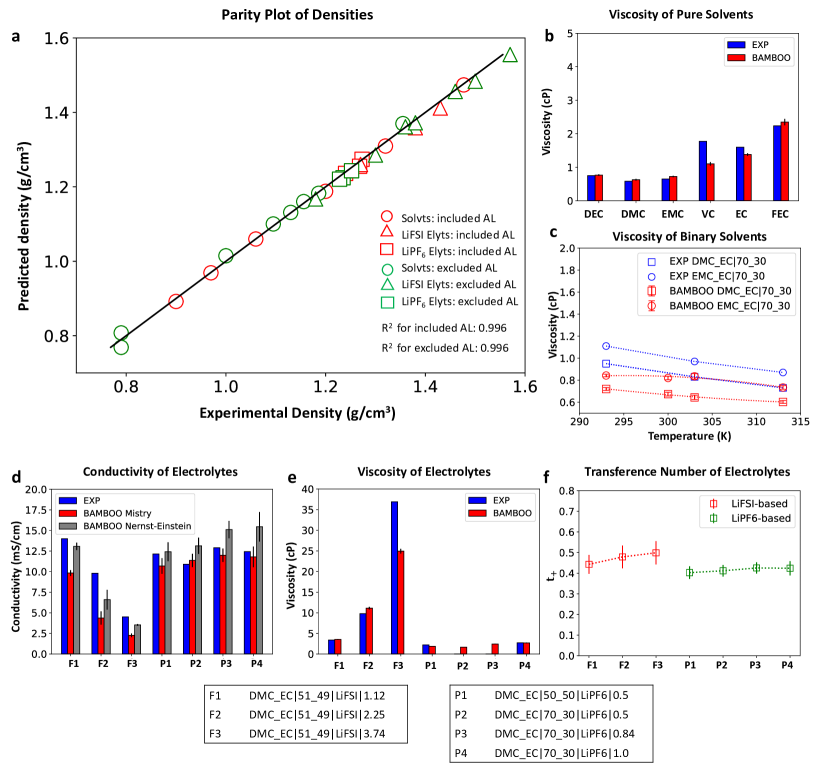
Figure 3: The predicted solvents and liquid electrolytes’ properties using BAMBOO. a. The parity plot comparing the predicted and experimentally measured densities of pure solvents, solvent mixtures, LiPF₆ and LiFSI containing electrolytes. “AL” in the legend represents the density “alignment” treatment. b. The predicted viscosity of common solvents compared to experimental measurements. c. Comparing the predicted viscosity of DMC-EC and EMC-EC solvent mixtures as a function of temperature to experimental results. d. Comparing the predicted and experimental conductivity of 7 common liquid electrolytes. The conductivity values presented are obtained by analysing the simulated trajectories using Mistry’s method [70] and Nernst-Einstein equation, denoted as “BAMBOO Mistry” and “BAMBOO Nernst-Einsten”, respectively. e. The predicted and experimental viscosity of the 7 electrolytes presented. f. The predicted cation transference number calculated using self-diffusion coefficients of Li⁺ and anions of the 7 electrolytes. The tables below panels d-f describe the electrolyte composition in “solvents$|$solvent weight $\%$$|$salt$|$salt molality” format. All data are tabulated in Table S5-S9 in the Supplementary Information.

In Figure 3, we present the predicted physical properties of solvents and electrolyte properties using BAMBOO compared with available experimental measurements. Figure 3a displays a parity plot between the experimental and predicted densities. As detailed above, the “alignment” process, denoted as “AL” in the figure, uses a set of selected experimental densities to finetune, thereby, enhancing the accuracy of density prediction. As expected, such alignment is also effective in improving the prediction accuracy beyond density due to physical property interconnection (demonstrated in Figure S9). It is crucial to emphasize that the alignment process does not necessitate the inclusion of experimental densities from all systems of interest. Instead, one can strategically choose representative systems, leveraging the transferability of the model. To encompass a broad spectrum, our alignment process includes linear and cyclic carbonates, esters, LiPF₆ based and LiFSI based binary to ternary electrolytes. Solvents and electrolytes excluded in the alignment process composed the same categories except for the solvents listed in “others” of Figure S1. All experimental and predicted densities are presented in Table S5 and S6 in the Supplementary Information.

To differentiate the alignment treatment, we use red and green markers in Figure 3a to indicate the systems that are included and excluded from the alignment process, respectively. Despite the differing treatments, both sets of data exhibit high R² values of 0.996, indicating excellent agreement between the predicted and experimental values. We observe that the densities of most linear solvents cluster below 1.2 g/cm³, whereas those of cyclic solvent species typically register higher values. Notably, the presence of the “C-F” functional group leads to an increase in solvent density. This density trend by solvent category follows chemical intuition. The densities of LiPF₆-based electrolytes aggregate between 1.2 g/cm³ to 1.3 g/cm³, reflecting the consistent presence of roughly 1m salt (molality, in mol/kg) in these electrolytes for which experimental values were available. In contrast, experimental data for LiFSI-based electrolytes span a wider concentration range, from 0.49m to 3.74m, resulting in a broader spread of densities from 1.2 g/cm³ to 1.6 g/cm³. Furthermore, our model predicts the densities of EO (CH₃CH₂OH) and ACT (CH₃-CO-CH₃) with good accuracy despite their structural differences from those included in “AL”. This results may be attributed to the transferability of the training and the alignment process using ethyl acetate (EA, CH₃COOC₂H₅) and other linear solvent species, underscoring a unique transferability feature of BAMBOO.

Figure 3b and 3c illustrate the predicted viscosity values for both pure solvents and binary solvent mixtures, respectively. We specially selected these solvents to address the broader interests of the Li battery electrolyte community. In examining pure solvents, we observe good agreements between the predicted viscosity values for linear solvents (DEC, DMC, and EMC) and experimental measurements. However, some discrepancies are apparent for cyclic carbonates, particularly VC, where the MLFF underestimates its viscosity by 0.67 cP. It’s important to acknowledge that experimental viscosity values reported in the literature for the same solvent can vary significantly. For instance, the reported viscosities for FEC at 40^∘C range from 2.24 cP to 4.1 cP [65, 64, 66]. Therefore, while discrepancies exist, it remains uncertain whether the performance of BAMBOO on some carbonates is accurately assessed using the available experimental results. Nevertheless, we can confidently assert that the differences in viscosity stemming from the categories of solvents are accurately captured by BAMBOO. Specifically, linear carbonates consistently exhibit lower viscosity compared with cyclic carbonates.

In Figure 3c, we showcase the predicted binary solvent viscosity (red markers) for DMC:EC 70:30 wt$\%$ and EMC:EC 70:30 wt$\%$ as a function of temperature, contrasted with experimental results (blue markers) reported by Logan $et$ $al.$ [69]. Notably, the decreasing trend depicted by the predicted values mirrors the experimental measurements. However, a consistent underestimation of viscosity by 0.2 cP is evident. Nonetheless, despite the underestimation, BAMBOO describes the trend such that EMC-EC viscosity exceeds DMC-EC.

Figure 3d and 3e show the conductivity and viscosity of 7 selected LiFSI- and LiPF6-based electrolyte blends. Among these, the three LiFSI based electrolytes are selected to demonstrate the variations in properties with salt concentration. Meanwhile, the inclusion of four LiPF₆-based electrolytes aims to emphasize changes resulting from different solvent bases while maintaining a fixed salt concentration, as well as variations arising from different salt concentrations while keeping the solvent constant. This design is to emphasize trends and correlations in transport properties. It is known that conductivity and viscosity have strong correlation, such that, the lower the viscosity, the higher the conductivity. This correlation is also widely used in designing fast charging liquid electrolytes [71, 69, 72]. Two methods are used to calculate conductivity, that are a method described by Mistry $et$ $al.$  [70] that uses Stefan-Maxwell diffusivities, while the other is the well-known Nernst-Einstein (NE) relation (equation 60 in the Supplementary Information) that uses self-diffusivities of the positive and the negative ions, ignoring ion-pairing and molecules’ correlated motion in simulation. Due to the nature of diffusivity calculations, the conductivity via Mistry’s method for a typical liquid electrolyte will always be lower than the results from NE, but will converge to NE at extremely low salt concentration. Therefore, the consistent lower results by Mistry’s method manifest the fact that ion-pairing and correlated motion exist in the simulated electrolytes, consistent with our solvation structure fraction observations in Figure 4.

In Figure 3d, moving from left to right, we observe a decrease in the experimental conductivity of LiFSI-based electrolytes (F1, F2, and F3) with increasing salt concentration. This trend is effectively captured by conductivities calculated using both methods; however, Mistry’s method exhibits a larger underestimation compared to NE. The associated atomic charge distributions for these three electrolytes are presented in Figure 4 to illustrate charge evolution as a function of concentration. Regarding LiPF₆-based electrolytes (P1-P4), Mistry’s method yields considerably more accurate results than NE. When considering error bars, the predicted results align well with the experiments. In contrast, NE estimated-conductivities of P3 and P4 are much higher than P1 and P2, though the differences across all four blends (P1-P4) are not significant.

Figure 3e shows the predicted viscosities of electrolyte blends F1-F3 and P1-P4. Despite discrepancies in the calculated conductivities of F1-F3 compared with experimental results, the predicted viscosities generally align well with experiments, with the exception of F3. Nonetheless, BAMBOO effectively captures the increasing viscosity trend as the salt concentration rises. Experimental viscosity data for P1-P4 are limited. However, the available results indicate that BAMBOO successfully reproduces experimental viscosities for P1 and P4, consistent with its conductivity performance.

We extract self-diffusivities ($D_{\pm,\text{self}}$) of Li⁺ and anions from the simulated MD trajectories and subsequently computed the cation’s transference number. The results are tabulated in Table S9 in the Supplementary Information. The transference number is defined as the ratio of $D_{+,\text{self}}$ over the summation of $D_{+,\text{self}}$ and $D_{-,\text{self}}$ as shown in equation 58. Our calculation shows that the t${}_{\text{Li}^{+}}$ for LiPF₆-based electrolytes are consistent around 0.4. This finding is in line with existing literature, which reports t${}_{\text{Li}^{+}}$ between 0.3 and 0.4 when measured using Bruce-Vincent or pfg-NMR techniques for state-of-the-art carbonate-based electrolytes [73]. For LiFSI-based electrolytes, we observed that the t${}_{\text{Li}^{+}}$s are slightly higher than those in LiPF₆-based electrolytes, consistent with prior research comparing LiPF₆ and LiFSI in carbonate solvents [74, 75]. Furthermore, we noted an increase in $t_{\text{Li}^{+}}$ for LiFSI-based electrolytes as the concentration rises from 1.12m to 3.74m. This observation aligns with the increasing formation of CIPs and AGGs, as illustrated in Figure 4. As the fractions of paired ions increase, the self-diffusivities of cations and anions become more correlated, leading the calculated t${}_{\text{Li}^{+}}$ to approach 0.5.

2.5 Solvation Structures and Atomic Partial Charges

Figure 4: The atomic charge distributions and the solvation structure fractions of three simulated LiFSI electrolytes using BAMBOO. a, b, and c, arranged from left to right, the Li charge histograms of 1.12m, 2.25m, and 3.74m LiFSI in a DMC:EC mixture of 51:49 wt$\%$. “m” denotes molality in mol/kg. Dotted lines within each panel, progressing from left to right, denote the Li charge distributions correlated with SSIP, CIP, and AGG solvation structures. Panels d, e, and f, organized from left to right, the O${}_{\text{FSI}^{-}}$ charge histograms illustrate the behavior within the three LiFSI electrolytes. Notably, the first dotted line may correlates to the distributions of paired O${}_{\text{FSI}^{-}}$. The second and third lines represent the two distinguished O${}_{\text{FSI}^{-}}$ charges linked to distributions of unpaired intra-molecular interactions. The charge values associated with the peaks from left to right are tabulated in legends as shown in each panel.

In Figure 4, we present the Li⁺ and O${}_{\text{FSI}^{-}}$ charge histograms derived from simulations of three distinct LiFSI electrolytes (F1-F3) spanning from 1.12m to 3.74m. The histograms of all the other atoms of FSI^- are presented in Figure S10. The peak locations of the red dotted lines in each figure panel are performed using the find-peaks function from the scipy.signal module. The weight ratio of DMC to EC, set at 51:49 wt$\%$, remains consistent across all these electrolytes.

Three distinct normal distributions can be observed in Figure 4a, each characterized by peaks intersecting the X-axis (Li⁺ charges) at approximately 0.622, 0.626, and 0.632, respectively. As we transit from Figure 4a to Figure 4c, these normal distributions in each figure panel and their peak locations roughly persist, albeit with varying heights. Specifically, the highest peak undergoes a shift from approximately 0.632 to 0.622 as the LiFSI concentration increases from 1.12m to 3.74m.

This shift in Li⁺-charge normal distributions is a manifest of the evolving solvation structure populations across different salt concentrations. To demonstrate this interpretation, we analyze the frames of the final 3 ns of MD simulations, and examine solvation structures around Li⁺s. The solvation structure types and their fractions are tabulated and shown under each Li⁺-charge histogram. These fractions are derived by first analyzing the radial distribution of the simulation trajectory for the radius of the first solvation shell around Li⁺, followed by extracting the central Li⁺ ions along with the surrounding solvated molecules. We find the first solvation shell has radius around 2.2 Å and the coordination number in all three systems are around 4 as shown in Figure S11 of the supporting information.

In general, the solvation structures can be categorized to SSIP, CIP and AGG. SSIPs denote structures composed solely of solvent molecules, in this case, EC and DMC. CIPs represent the structures containing one anion-in this context, FSI^- within the first solvation shell. Finally, AGGs refer to collective structures composed of more than one anion in the first solvation shell. Our analysis reveals SSIP ratios of 0.751, 0.494 and 0.182 for LiFSI concentrations of 1.12m, 2.25m, and 3.74m, respectively. CIP ratios are 0.171, 0.260, and 0.276; AGG ratios are 0.078, 0.246 and 0.542. The ratio differences among SSIPs, CIPs, and AGGs in each figure panel and their changes as a function of salt concentrations roughly mirror the peak height evolution depicted from Figure 4a to 4c. It is important to note that our goal in this analysis is not to separate the contributions of different solvation structures to atomic partial charge histograms. Therefore, a detailed fitting involving integrating areas below each peak is unnecessary.

It is well known that solvation interactions between Li⁺ ions and surrounding molecules, including solvents and anions, primarily occur through Li⁺-O interactions in LiFSI-based carbonate electrolytes. These intermolecular interactions may lead to polarization-induced partial charge changes within the local solvation environment. To demonstrate this, besides analyzing Li⁺s, we also examine atomic charge distributions across all atom types within the FSI^- anion. Interestingly, we observe that O${}_{\text{FSI}^{-}}$ exhibits three overlapping normal distributions as shown in Figure 4d-f, whereas the other atom types display single normal distributions for all concentrations as presented in Figure S10.

As depicted in Figure 4d, it is evident to identify two peaks (the right and middle), which are highlighted with the red dotted lines. We posit these peaks originate from two types of Oxygen atoms within the FSI^- molecule. This hypothesis stems from our observation that at 1.12m LiFSI concentration, most of the anions should remain unpaired due to low CIP and AGG fractions. In addition, these unpaired anions are likely not solvated by solvent molecules. In lithium battery electrolytes, solvents such as EC and DMC are designed to primarily solvate positive ions, resulting in anions often free from solvent-anion inter-molecular interactions [2]. Consequently, the two prominent normal distributions with peak locations around -0.370 and -0.360 are indicative of potential intra-molecular differences in O${}_{\text{FSI}^{-}}$s of free FSI^- in the simulated 1.12m LiFSI electrolyte. An additional peak, highlighted with the yellow dotted line in Figure 4d, is visually identified based on its similarity in charge location compared to Figure 4e and 4f. We observe this peak progressively becomes more prominent as the concentration increases from 1.12m to 3.74m. We hypothesize that this peak is associated with ion-pairing, as the growth in peak height correlates the increasing total fractions of CIP and AGGs. Although CIP and AGG represent distinguishable solvation structures with respect to Li⁺ ions, they may not be differentiated from the perspective of O${}_{\text{FSI}^{-}}$s.

We observe that with increasing concentration, there is a rise in the fraction of Li ions with lower atomic charges. O${}_{\text{FSI}^{-}}$ also shows such a trend. This observation may initially appear counter-intuitive, as it suggests the Li charge decreases did not end up being taken by O${}_{\text{FSI}^{-}}$s. Upon analyzing the charge histograms of N, F, and S in Figure S10, we observe consistent shifts in the normal distribution peaks from more negative to more positive values. These shifts, totaling 0.014, likely indicate that atomic charges moved away from Li ions being compensated by N, F, and S, along with other solvent molecules.

The results presented here demonstrate the charges of Li⁺ and other atomic species are not fixed, rather, they changes as electrolyte compositions. In liquid electrolyte simulations, particularly in applications involving lithium batteries, accurately capturing polarizability is crucial for describing Li⁺ transport properties. However, classical force fields often fall short in this aspect. A typical treatment in classical MD using a non-polarizable force field is to scaling the ions’ and solvents’ charges [76, 77] to match experimental properties, such as self-diffusivities for specific systems of interest. The goal is to provide a mean-field representation of charge screening [78]. However, different scaling factors are required when investigating different electrolyte chemistries or compositions, leading to limited generalizability. Determining the optimal charge scaling scheme typically relies on Li⁺ self-diffusivity data obtained from Nuclear Magnetic Resonance Spectroscopy (NMR) [77], which can be costly and time-consuming, sometimes defeat the purpose of novel liquid electrolyte exploration. Therefore, given the generalizability and flexibility of BAMBOO in providing solvation insights, there exists an unique opportunity for MLFF to participate in “bottom-up” understanding [78] and design of liquid electrolytes.

2.6 Transferability to Unseen Molecules

Figure 5: Transferability of BAMBOO to unseen fluorinated molecules. a, b. Illustration of fluorinated EC molecules and densities of the EC derivatives from BAMBOO and experiment, respectively. c, d. Illustration of fluorinated DMC molecules and densities of the DMC derivatives from BAMBOO and experiment, respectively. e, f. Illustration of fluorinated EA molecules and densities of the EA derivatives from BAMBOO and experiment, respectively.

In this section, we show the transferability of BAMBOO to solvents that are excluded in the DFT training dataset. In advanced electrolytes, fluorination of a base solvent is a commonly used strategy [79, 80] to enhance electrochemical performance [81], LiF-rich SEI formation [82], and fire-resisting property [83]. Despite the popularity and effectiveness of fluorination, the exact relationship of the location and the degree of fluorination to the liquid electrolyte performances are not clear. This underscores the importance to incorporate MLFF in structural-based electrolyte design.

To satisfy the potential interest in exploring novel solvent derivatives completely in silico, we assess the generalizability of our current model to unseen molecules, probing its capability limitations and providing guidance for further improvement. The parent molecules, EC, DMC, and EA and their derived child molecular structures are shown in Figure 5a, c, and e. All child molecules are excluded from training or alignment, except for FEC. The same BAMBOO model used for generating the liquid electrolyte properties shown in Figure 3 is used in the transferability study. We find all simulations of the child solvents remain stable during the 5 ns MD simulations within a broad temperature range 283-343 K, demonstrating the high transferability of the model.

In Figure 5b, d, and f, we present the simulated densities of the fluorinated derivatives from BAMBOO MD simulations and experiments as a function of temperatures. Qualitatively, we find that, except for the fluorinated EAs (FEA, EFA), which have very similar structures and experimental densities, BAMBOO can correctly predict the density trends of fluorinated ECs and DMCs. To be specific, the trend cis-DFEC $>$ DFEC $>$ trans-DEFC, and the trend FDMC $>$ DFDMC $>$ MFDMC are reproduced. The trend for DMC derivatives follows the intuition that as the fluorination increases, density increases. In addition, we find that the more structural-alike the unseen child molecule compared with the parent molecule, the more accurate the prediction of density from BAMBOO is. Furthermore, the inclusion of the functional group of interest in training data is crucial for accuracy. For instance, since FEC is already included in the DFT dataset, the density discrepancy of other fluorinated derivatives of EC from BAMBOO are within 0.03 g/cm³ compared with that from experiments. As a comparison, since there is no fluorinated derivative of EA and DMC in the DFT dataset, the density errors of the simulated results for fluorinated EA and DMC are generally at the order of 0.1 g/cm³, which is larger than that of fluorinated EC. Specifically, with higher degree of fluorination, we can see that the density error of DMC’s child molecules becomes larger, from around 0.05 g/cm³ for MFDMC, 0.08 g/cm³ for DFDMC, to 0.20 g/cm³ for TFDMC. The comparison between EC and DMC derived molecules indicate that BAMBOO has the potential to transfer to unseen molecules in terms of calculating density but requires small amount of DFT training data describing the specific functional groups and types of molecular backbone. Here, we speculate the accuracy of density predictions to the fluorinated EAs and DMCs can be improved by including “-CH₂F” and “-CHF₂” functional groups in the DFT dataset, which will be incorporated in a later version of BAMBOO.

3 Discussions

In summary, this study presents a machine learning force field framework-BAMBOO, tailored for MD simulations of liquid electrolytes. First, we devise a GET architecture that segregates semi-local, electrostatic, and dispersion interactions, leveraging insights from DFT calculations. Second, we pioneer ensemble knowledge distillation on MLFF, ensuring the stability of MD simulations based on MLFF. Moreover, we introduce a novel physics-based alignment approach to reconcile simulated density with experimental data, thus establishing a connection between macroscopic and microscopic scales. Our results demonstrate the effectiveness of the density alignment process in reducing disparities between simulated and experimental outcomes, extending its benefits to properties beyond density. To further enhance the model’s performance in predicting properties beyond density, such as conductivity, simultaneous and direct alignment of these additional properties is essential. Hence, our future endeavors will be dedicated to expanding the alignment process to encompass a wider spectrum of properties.

We conduct a comprehensive assessment for BAMBOO model’s performance on solvents and liquid electrolytes. Our simulated results demonstrate that a single BAMBOO model can predict densities, viscosities, and ionic conductivities for a broad range of chemistries with high accuracy. The current BAMBOO model is able to simulate up to 15 species in various compositions. This robustness underscores BAMBOO’s value in facilitating design and optimization of practical liquid electrolytes, which may contain up to 10 components. Notably, BAMBOO’s generalizability sets it apart from classical force field models, which often rely on ad hoc adjustments and struggle to achieve simultaneous accuracy across multiple liquid electrolyte components. In addition to the state-of-the-art bulk property prediction accuracy, we also show the quantification of the relationship between solvation structures and atomic partial charges as a function of electrolyte compositions, providing insights for solvation engineering that are unreachable by classical force fields or DFT. Furthermore, our transferability analysis demonstrates BAMBOO’s efficacy in exploring novel solvents, even in the absence of specific DFT training data. To enhance BAMBOO’s transferability to unseen molecules, particularly those with novel functional groups, pretraining on large molecule databases containing millions of diverse structures could be advantageous. We envision this work as laying the foundation for the development of “universal machine learning force fields” capable of accurately simulating bulk properties of all organic liquids.

4 Acknowledgement

The authors acknowledge insightful ion transport theory discussion with Aashutosh Mistry, assistant professor at Colorado School of Mines. The authors also acknowledge the experimental data points provided by Adarsh Dave, former PhD student at Carnegie Mellon University, upon request.

4.1 Author Contributions

Conceptualization: Y.Z., W.Y., W.G., Z.M, Z.Y., S.G., T.Z., Z.W., L.C., X.W., S.S., and L.X.; Methodology: S.G., Y.Z., Z.M., Z.P., H.W., and W.G.; Investigation: S.G., Y.Z., Z.M., Z.P., H.W., M.C., and W.G.; Supervision: W.G., W.Y., and L.X.; Writing: S.G., Y.Z., Z.M., Z.P., H.W., W.Y., and W.G.

4.2 Conflict of Interests

ByteDance Inc. holds intellectual property rights pertinent to the research presented herein. Furthermore, the innovations described have resulted in the filing of a patent application in China (Patent Application No. 202311322469.2), which is currently pending.

5 Data and code availability

The DFT datasets of clusters, the final trained, ensemble knowledge distilled, and density aligned model of BAMBOO to reproduce the results in the paper, as well as the source codes, are provided in the referenced link [84].

Supplementary Information

BAMBOO: a predictive and transferable machine learning force field framework for liquid electrolyte development

Table of Contents

[supplement] [supplement]l1

Appendix A Details of Initial Training by DFT Data

A.1 Graph Equivariant Transformer

Given atomic structures, we first initialize node scalar representation $x_{i}^{0}$ and node vector representations $\vec{V}_{i}^{0}$ for atom $i$ based on the atom type $z_{i}$, and initialize edge scalar representation $d_{ij}$ and edge vector representation $\vec{e}_{ij}$ based on the relative vector between atom $i$ and atom $j$ ($\vec{r}_{ij}$) within a certain cut off radius $r_{\text{cut}}$ (5Å in this work):

$$x_{i}^{0}=\text{embeddingMLP}(z_{i}),$$ (1)

$$\vec{V}_{i}^{0}=\vec{0},$$ (2)

$$\hat{r}_{ij}=\frac{\vec{r}_{ij}}{||r_{ij}||},$$ (3)

$$d_{ij}=\text{SiLU}(W^{d}\text{RBF}(||r_{ij}||)),$$ (4)

$$\vec{e}_{ij}=\text{SiLU}(W^{e}d_{ij})^{T}\otimes\hat{r}_{ij}.$$ (5)

Here, embeddingMLP is a multi-layer perceptron (MLP) that maps discrete atom types into continuous embeddings implemented in the nn.Embedding class in PyTorch [85], $||\cdot||$ is the L2 norm of a vector, RBF is the radial distribution functions-based expansion as in Ref. [86] that expands distance into high-dimensional representations, and SiLU refers to the Sigmoid-Weighted Linear Units [87] activation function. In equation (4) and (5), $W^{d}$ and $W^{e}$ refers to the weight matrix used to generate $d_{ij}$ and $\vec{e}_{ij}$, respectively.

After initialization, we input $x_{i}^{0}$, $\vec{V}_{i}^{0}$, $d_{ij}$, $\vec{e}_{ij}$ into the GET layers. In the n^th layer, we first input $x_{i}^{n}$ into a LayerNorm [88] layer, then we input $x_{i}^{n}$, $||r_{ij}||$, and $d_{ij}$ into the classic QKV-transformer shown in Figure 1e and described as below:

$$q_{i}^{n}=W^{q,n}x^{n}_{i}+b^{q,n},$$ (6)

$$k_{i}^{n}=W^{k,n}x^{n}_{i}+b^{k,n},$$ (7)

$$v_{i}^{n}=W^{v,n}x^{n}_{i}+b^{v,n}.$$ (8)

Here $q_{i}^{n}$, $k_{i}^{n}$, and $v_{i}^{n}$ are queries, keys and values in transformer [51] (notice that capital $V$ stands for vector embedding whereas lowercase $v$ stands for “values” in QKV-attension). We further compute the attention weight $a_{ij}^{n}$ and the intermediate node scalar representation $y_{i}^{n}$. Furthermore, we build an intermediate vector representation $\vec{u}_{ij}^{n}$ to incorporate edge vector representation $\vec{e}_{ij}$ into the GET layer and sum contributions of neighboring atoms to the vector representation.

$$a_{ij}^{n}=\frac{1}{2}\text{SiLU}(\langle q_{i}^{n},k_{j}^{n}\rangle)(\cos{\frac{\pi||r_{ij}||}{r_{\text{cut}}}+1}),$$ (9)

$$y_{i}^{n}=\sum_{j}a_{ji}^{n}(v_{j}^{n}\odot d_{ij}),$$ (10)

$$\vec{u}_{i}^{n}=\sum_{j}v_{j}^{n}*\vec{e}_{ij}.$$ (11)

Here, $\odot$ is element-wise multiplication and “$*$” as the following multiplication operation to combine a scalar $A\in R^{m}$ and a vector $\vec{B}\in R^{m\times 3}$ which keeps equivariance of $\vec{B}$.

$$A*B =\begin{bmatrix}A_{1}\\ A_{2}\\ \vdots\\ A_{m}\end{bmatrix}*\begin{bmatrix}B_{11},B_{12},B_{13}\\ B_{21},B_{22},B_{23}\\ \vdots\\ B_{m1},B_{m2},B_{m3}\end{bmatrix}=\begin{bmatrix}A_{1}B_{11},A_{1}B_{12},A_{1}B_{13}\\ A_{2}B_{21},A_{2}B_{22},A_{2}B_{23}\\ \vdots\\ A_{m}B_{m1},A_{m}B_{m2},A_{m}B_{m3}\end{bmatrix}.$$ (12)

For the vector embeddings, we first update node vector representation $\vec{V}_{i}^{n}$ by linear projection:

$$\vec{U}_{i}^{1,n}=W^{U^{1},n}\vec{V}_{i}^{n},$$ (13)

$$\vec{U}_{i}^{2,n}=W^{U^{2},n}\vec{V}_{i}^{n},$$ (14)

$$\vec{U}_{i}^{3,n}=W^{U^{3},n}\vec{V}_{i}^{n}.$$ (15)

Then, we use inner product $\langle\cdot,\cdot\rangle$ to generate the scalar representation $w_{i}^{n}\in R^{m}$ from $\vec{U}_{i}^{1,n}$, $\vec{U}_{i}^{2,n}\in R^{m\times 3}$, which is consequently used to interact with the intermediate node scalar representation $y_{i}^{n}$:

$$w_{i}^{n}=\langle\vec{U}_{i}^{1,n},\vec{U}_{i}^{2,n}\rangle.$$ (16)

Before final output, we further transform $y_{i}^{n}$ into three species:

$$O_{i}^{1,n}=W^{O^{1},n}y_{i}^{n}+b^{O^{1},n},$$ (17)

$$O_{i}^{2,n}=W^{O^{2},n}y_{i}^{n}+b^{O^{2},n},$$ (18)

$$O_{i}^{3,n}=W^{O^{3},n}y_{i}^{n}+b^{O^{3},n}.$$ (19)

Finally, we output the updated node scalar representation $x_{i}^{n+1}$ and node vector representation $\vec{V}_{i}^{n+1}$ for the $(n+1)^{th}$ layer:

$$x_{i}^{n+1}=x_{i}^{n}+\langle\vec{U}_{i}^{1,n},\vec{U}_{i}^{2,n}\rangle\odot O_{i}^{2,n}+O_{i}^{3,n},$$ (20)

$$\vec{V}_{i}^{n+1}=\vec{V}_{i}^{n}+O_{i}^{1,n}*\vec{U}_{i}^{3,n}+\vec{u}_{i}^{n}.$$ (21)

As above, both of the node scalar and vector representations in the $(n+1)^{th}$ layer encode both scalar and vector information from both node and edge in the $n^{th}$ layer. The importance of the equivariant vector information and the transformer architecture is shown in Section D below.

In this work, we refrain from calculating many-body features like bond angles and dihedral angles for two main reasons. Firstly, the GET layer in our model inherently captures all many-body effects [89] with its infinite body-order, as defined by the derivative-based understanding of many-body interactions. This means that the many-body phenomena are implicitly represented. Secondly, referencing the findings from another study [90], introducing explicit three-body terms into transformer-based graph neural networks doesn’t significantly enhance the prediction of atomic structure properties, yet it substantially increases computational demand. Additionally, we avoid using tensor products to maintain rapid inference speeds, given that tensor operations are known for their slow speed.

A.2 Separation of Interactions

Once we reach the final GET layer (n^th layer as below, and n=3 in this work), we compute NN-based per atom energy $E_{i}^{\text{NN}}$ and atomic partial charges $q_{i}$ based on $x_{i}^{n}$ by two MLPs:

$$E_{i}^{\text{NN}}=\text{MLP}^{\text{energy}}(x_{i}^{n}),$$ (22)

$$q_{i}=\text{MLP}^{\text{charge}}(x_{i}^{n}),$$ (23)

and we compute NN-based forces by:

$$\vec{f}_{ij}^{\text{ NN}}=\frac{1}{2}(-\frac{\partial E^{\text{NN}}}{\partial r_{ij}}+\frac{\partial E^{\text{NN}}}{\partial r_{ji}}),\vec{f}_{i}^{\text{ NN}}=\sum_{j\neq i}\vec{f}_{ji}^{\text{ NN}}.$$ (24)

Then, we define the electrostatic energy model based on the charge equilibrium theory [48]:

$$E^{\text{elec}}=\sum_{i}\chi_{i}q_{i}+\frac{1}{2}\sum_{i,j}\frac{q_{i}q_{j}}{r_{ij}}+\frac{1}{2}\sum_{i}J_{i}q_{i}^{2}.$$ (25)

Here, $\chi_{i}$ is the element-wise electronegativity, and $J_{i}$ is the element-wise electronic hardness. The reason behind why we do not predict $\chi$ and $J$ based on structures is stated in the proof of Theorem 35 in the next section. In this work, both of the two quantities only depend on atomic types and are learned and predicted by MLPs:

$$\chi_{i}=(\text{MLP}^{\chi}(x_{i}^{0}))^{2},$$ (26)

$$J_{i}=(\text{MLP}^{\text{J}}(x_{i}^{0}))^{2}.$$ (27)

Here we use the square of the outputs of the two MLPs to ensure that both of the two quantities are positive. More discussion about charge equilibrium is provided in the next section.

In addition, given atomic structures, we can directly compute dispersion interaction ($E_{i}^{\text{disp}}$ and $\vec{f}_{i}^{\text{ disp}}$) by the D3 correction [49]. Note that we do not include dispersion correction in the DFT training data and therefore do not consider $E_{i}^{\text{disp}}$ and $\vec{f}_{i}^{\text{ disp}}$ in the whole training process. We only incorporate dispersion correction in BAMBOO during MD simulations. Finally, we combine NN, electrostatic, and dispersion interactions to compute the total energy and force of each atom:

$$E_{i}^{\text{total}}=E_{i}^{\text{NN}}+E_{i}^{\text{elec}}+E_{i}^{\text{disp}},$$ (28)

$$\vec{f}_{i}^{\text{total}}=\vec{f}_{i}^{\text{NN}}+\vec{f}_{i}^{\text{elec}}+\vec{f}_{i}^{\text{disp}}.$$ (29)

We further compute the virial tensor T based on pairwise forces:

$$\vec{f}_{ij}=\vec{f}_{ij}^{\text{NN}}+\vec{f}_{ij}^{\text{elec}}+\vec{f}_{ij}^{\text{disp}},$$ (30)

$$\textbf{T}=\sum_{i}^{N}\sum_{j}^{N}\vec{f}_{ij}\otimes\vec{r}_{ij},$$ (31)

where $\otimes$ is the outer product between the two 3-dimensional vectors. Here, according to equation (24) and (33) and the nature of $\vec{f}_{ij}^{\text{disp}}$, $\vec{f}_{ij}=-\vec{f}_{ji}$, which satisfies the Newton’s Third Law of opposite forces for computing the microscopic stress [50], and since we compute $\vec{r}_{ij}$ across periodic boundary, we do not need additional correction for computing T of periodic systems. We also compute the dipole moment as $\vec{D}=\sum_{i=1}^{N}q_{i}\vec{r}_{i}$ for training the machine learning model.

A.3 Charge Equilibrium

It has been well-known that a fixed-charge model may impose serious restrictions on the fidelity and transferability of force fields. However, allowing charges to vary throughout a molecular dynamics simulation is non-trivial. Partial charge is an abstraction of electron density and should reflect the fact that electron density is at electrostatic equilibrium at any moment. If we arbitrarily change the charge in a MD simulation, we are actually pumping energy into (or dissipating energy from) the system and violating the basic energy conservation law that is necessary to collect correct statistical results from the simulations. Therefore, the charges should be allowed to change to reflect the necessary physics but also restricted to obey the physical laws. This is the central topic of polarizable force fields, and many different approaches have been developed in the past decades for different systems [91, 92].

In this work, we incorporate the charge equilibrium model (Qeq here after) into our MLFF for its efficiency. We further use a strong regularization strategy to make our GNN model directly outputs the Qeq charges such that an expensive iterative equilibrium solver per MD timestep is completely removed. By definition, the force associated with the electrostatic energy should be:

$$\vec{f}_{i}^{\text{elec*}}=-\frac{\partial E^{\text{elec}}}{\partial r_{i}}=-\sum_{j}\frac{q_{i}q_{j}}{r_{ij}^{2}}\hat{r}_{ij}+\sum_{i}\chi_{i}\frac{\partial q_{i}}{\partial r_{i}}+\frac{1}{2}\sum_{i,j}\frac{1}{r_{ij}}\frac{\partial(q_{i}q_{j})}{\partial r_{i}}+\frac{1}{2}\sum_{i}J_{i}\frac{\partial q_{i}^{2}}{\partial r_{i}}.$$ (32)

Although for non-periodic systems, $\partial E^{\text{elec}}/\partial r_{i}$ is straightforward to compute by auto-differentiation in PyTorch [85], for periodic boxes in MD simulations, most MD engines such as LAMMPS [53], can only compute Ewald summation [93] for the long-range electrostatic force defined as below:

$$\vec{f}_{i}^{\text{elec}}=-\sum_{j}\frac{q_{i}q_{j}}{r_{ij}^{2}}\hat{r}_{ij}.$$ (33)

Technically, it is difficult to explicitly compute the remaining terms in equation (32) as it is expensive to compute $\partial q_{j}/\partial r_{i}$ for all the pairs of atoms. To bypass such difficulty, we refer to the charge equilibrium theory [48].

In the following, we demonstrate that, under charge equilibrium, $\vec{f}_{i}^{\text{elec}}=\vec{f}_{i}^{\text{elec*}}$. To simplify the notations in the proof, in the following we introduce vector $\textbf{x}=\{\chi_{1},\dots\chi_{N}\},\textbf{x}\in R^{N}$, and matrix $\textbf{J}:J_{ij}=1/r_{ij},J_{ii}=J_{i},J\in R^{N\times N}$. We prove the following two theorems.

Theorem A.1

If $\textbf{q}=\{q_{1},\dots,q_{N}\},q\in R^{N}$, such that

$$\textbf{q}=\arg\min_{\textbf{q}}(E(\textbf{q})-\lambda(\sum_{i}q_{i}-q_{total})),$$ (34)

where $\lambda$ is the Lagrange multiplier to ensure that $\sum_{i}q_{i}=q_{total}$, then

$$\vec{f}_{i}^{\text{elec}}=-\frac{\partial E^{\text{elec}}}{\partial r_{i}}=-\sum_{j}\frac{q_{i}q_{j}}{r_{ij}^{2}}\hat{r}_{ij}.$$ (35)

Proof of Theorem A.1 We first define the target of minimization:

$$L(\textbf{q},\lambda)=\textbf{x}^{T}\textbf{q}+\frac{1}{2}\textbf{q}^{T}\textbf{J}\textbf{q}-\lambda(\textbf{1}^{T}\textbf{q}-q_{total}),$$ (36)

where 1 is a all-one vector. If q is a minimizer of $L$, then

$$0=\frac{\partial L}{\partial\textbf{q}}=\textbf{x}+\frac{1}{2}\textbf{J}^{T}\textbf{q}+\frac{1}{2}\textbf{J}\textbf{q}-\lambda\textbf{1}=\textbf{x}+\textbf{J}\textbf{q}-\lambda\textbf{1},$$ (37)

where the second ”=” is because J is symmetric. Similarly, we also have:

$$0=\frac{\partial L}{\partial\lambda}=q_{total}-\textbf{1}^{T}\textbf{q}.$$ (38)

Now we calculate $-\partial E^{\text{elec}}/\partial r_{i}$. To simplify the writing by avoiding 3-dimensional tensors, here we consider just one dimension of $\vec{r}_{i}$, for example, $z_{i}$,

$$\frac{\partial E}{\partial z_{i}}=\frac{\partial}{\partial z_{i}}(\textbf{x}^{T}\textbf{q}+\frac{1}{2}\textbf{q}^{T}\textbf{J}\textbf{q})=\frac{\partial\textbf{x}^{T}}{\partial z_{i}}\textbf{q}+\textbf{x}^{T}\frac{\partial\textbf{q}}{dz_{i}}+\frac{1}{2}\frac{\partial\textbf{q}^{T}}{\partial z_{i}}\textbf{J}\textbf{q}+\frac{1}{2}\textbf{q}^{T}\frac{\partial\textbf{J}}{\partial z_{i}}\textbf{q}+\frac{1}{2}\textbf{q}^{T}\textbf{J}\frac{\partial\textbf{q}}{\partial z_{i}}.$$ (39)

Here, the term $\frac{\partial\textbf{x}^{T}}{\partial z_{i}}\textbf{q}=0$, because $\chi$ does not depend on structures. The terms $\frac{1}{2}\frac{\partial\textbf{q}^{T}}{\partial z_{i}}\textbf{J}\textbf{q}$ and $\frac{1}{2}\textbf{q}^{T}\textbf{J}\frac{\partial\textbf{q}}{\partial z_{i}}$ can be combined into $\textbf{q}^{T}\textbf{J}\frac{\partial\textbf{q}}{\partial z_{i}}$ due to the symmetry of J. The fourth term $\frac{1}{2}\textbf{q}^{T}\frac{\partial\textbf{J}}{\partial z_{i}}\textbf{q}$ is the desired expression of $\vec{f}_{i}^{\text{elec}}$. For the remaining terms, we have:

$$\textbf{x}^{T}\frac{\partial\textbf{q}}{\partial z_{i}}+\textbf{q}^{T}\textbf{J}\frac{\partial\textbf{q}}{\partial z_{i}}=(\textbf{x}+\textbf{J}\textbf{q})^{T}\frac{\partial\textbf{q}}{\partial z_{i}}=\lambda\textbf{1}^{T}\frac{\partial\textbf{q}}{\partial z_{i}}=\lambda\frac{\partial(\textbf{1}^{T}\textbf{q})}{\partial z_{i}}=\lambda\frac{\partial q_{total}}{\partial r_{i}}=0.$$ (40)

where the second “$=$” is from equation (37), the fourth “$=$” is from equation (38), and the last “$=$” is because $q_{total}$ is a constant for a given system. Therefore, we have proved that:

$$\vec{f}_{i}^{\text{elec}}=-\frac{\partial E}{\partial z_{i}}=-\frac{1}{2}\textbf{q}^{T}\frac{\partial\textbf{J}}{\partial z_{i}}\textbf{q}.$$ (41)

Then, we prove the reverse theorem:

Theorem A.2

If $\textbf{q}=\{q_{1},\dots,q_{N}\},q\in R^{N}$ such that it satisfies equation (41), and $rank(\frac{\partial\textbf{q}}{\partial\textbf{c}})=N-1,c_{i}\in\{x_{1},y_{1},z_{1},\dots x_{N},y_{N},z_{N}\}$, then there exists $\lambda$ such that $\textbf{q}=\arg\min_{\textbf{q}}(E(\textbf{q})-\lambda(\sum_{i}q_{i}-q_{total}))$.

Proof of Theorem A.2 Combining equation (39), (41) and the fact that $\frac{\partial\textbf{x}^{T}}{\partial z_{i}}\textbf{q}=0$, we have:

$$\textbf{x}^{T}\frac{\partial\textbf{q}}{\partial z_{i}}+\textbf{q}^{T}\textbf{J}\frac{\partial\textbf{q}}{\partial z_{i}}=(\textbf{x}+\textbf{J}\textbf{q})^{T}\frac{\partial\textbf{q}}{\partial z_{i}}=0,$$ (42)

which can extend to all $c_{i}\in\{x_{1},y_{1},z_{1},\dots x_{N},y_{N},z_{N}\}$. We then combine all $\frac{\partial\textbf{q}}{\partial c_{i}}$ into a matrix with the dimensions of $3N\times N$, denoted as $\frac{\partial\textbf{q}}{\partial\textbf{c}}$. Because $\sum_{i}q_{i}=q_{total}$, therefore for all $c_{i}$, we have $\textbf{1}^{T}\frac{\partial\textbf{q}}{\partial c_{i}}=0$, and consequently $\frac{\partial\textbf{q}}{\partial\textbf{c}}^{T}\textbf{1}=\textbf{0}$. As a result, the rank of $\frac{\partial\textbf{q}}{\partial\textbf{c}}$ is at most $N-1$. If $rank(\frac{\partial\textbf{q}}{\partial\textbf{c}})=N-1$ as in the theorem, then due to equation (42), $\textbf{x}+\textbf{J}\textbf{q}$ is in the linear space spanned by 1. Therefore, there exists $\lambda$ such that $\textbf{x}+\textbf{J}\textbf{q}=\lambda\textbf{1}$, which also means $\frac{\partial L(\textbf{q})}{\partial\textbf{q}}=0$ where $L$ is defined in equation (36). Because $\frac{\partial^{2}L(\textbf{q})}{\partial\textbf{q}^{2}}=\textbf{J}$, where $J$ is a diagonally-dominant matrix with all positive diagonal elements, $\frac{\partial^{2}L(\textbf{q})}{\partial\textbf{q}^{2}}$ is a positive-definite matrix, therefore $L(\textbf{q})$ is a positive definite quadratic form of q, and q is the global minimizer of $L(\textbf{q})$.

From theorem 35, we know that the predicted charge q should satisfy equation (34) to ensure that $\vec{f}_{i}^{\text{elec}}$ is strictly conservative. However, in practice, to satisfy equation (34), the time complexity to compute matrix J is $\mathcal{O}(N^{2})$, and the time complexity to compute the inverse of J is $\mathcal{O}(N^{3})$. Since the time complexity of the GET layers is $\mathcal{O}(n)$, computing J and $\textbf{J}^{-1}$ would largely slow down the MD simulation for large systems with thousands of atoms. Moreover, since there is energy dissipation in the NPT and NVT ensembles used for studying liquid electrolyte in MD, small energy drift by non-conservative force would not affect results from MD simulations. In Ref. [39], the authors use a recursive method to approximate equation (34) with the time complexity of $\mathcal{O}(N)$. However, this recursive method would also slow down the inference speed, the degree of which depends on the number of iterations: the closer approximation, the more iterations, and the slower inference speed.

In this work, we design a method to approximate charge equilibrium in equation (34) with the minimum increase of inference speed, in which we decouple the inference speed with the degree of approximation. Instead of additional operations at inference, we move the approximation to the training process by adding a loss term in equation (44) to minimize the difference between $\vec{f}_{i}^{\text{elec}}$ and $\vec{f}_{i}^{\text{elec*}}$, which is an approximation to charge equilibrium as in Theorem A.2:

$$L_{\text{Qeq}}=||\vec{f}_{i}^{\text{elec}}-\vec{f}_{i}^{\text{elec*}}||^{2}.$$ (43)

Although this method seems straightforward as it directly minimizes the difference between the electrostatic force we can compute and the derivative of the electrostatic energy with respect to coordinates, equation (43) actually has the physical meaning of charge equilibrium as in the Theorems 35 and A.2. The degree of approximation depends on the magnitude of the weight factor of $\alpha_{Qeq}$ in the total loss as below. We show the importance of $\alpha_{Qeq}$ in Figure S2a, where smaller weight factors results in significant energy drift, while the largest weight factor only leads to 0.02 kcal/mol/atom energy increase in the 800 ps NVE simulation. This degree of energy drift is negligible in MD simulations with the NVT and NPT ensemble, as there is energy dissipation in this two ensembles. In Figure S2b and c, we show that the temperature of 1 ns NVT MD simulation and 4 ns NPT simulation slightly fluctuates around the set temperature of the simulation (303 K), and pressure around one atmosphere, which demonstrates the stability of the MD simulation. This method of charge equilibrium regularization minimally increases the inference speed by adding two summation over atoms as in equation (25).

Figure S2: a Energy drift in molecular dynamics simulations by NVE ensemble. The simulated system is EC$|$LiPF6$|$0.95. b and c Temperature and pressure versus simulation time of DMC$\_$EC$|$51$\_$49$|$LiFSI$|$0.49, respectively.

A.4 Initial Training of BAMBOO

Given the design of the GET architecture and the prediction of energy, force, virial and dipole, we use the following loss function to train the neural networks in BAMBOO:

$$\begin{split}L_{\text{training}}=\frac{1}{N_{\text{cluster}}}\sum_{k}^{N_{\text{cluster}}}\sum_{i}^{N_{\text{atom}}}&(\alpha_{\text{energy}}^{\text{training}}(E_{k}^{\text{DFT}}-E_{k}^{\text{BAMBOO}})^{2}\\ &+\frac{1}{N_{\text{atom}}}\alpha_{\text{force}}^{\text{training}}||\vec{f}_{k,i}^{\text{DFT}}-\vec{f}_{k,i}^{\text{BAMBOO}}||^{2}\\ &+\alpha_{\text{virial}}^{\text{training}}||\textbf{T}_{k}^{\text{DFT}}-\textbf{T}_{k}^{\text{BAMBOO}}||^{2}\\ &+\frac{1}{N_{\text{atom}}}\alpha_{\text{charge}}^{\text{training}}(q_{k,i}^{\text{DFT}}-q_{k,i}^{\text{BAMBOO}})^{2}\\ &+\alpha_{\text{dipole}}^{\text{training}}||\vec{D}_{k}^{\text{DFT}}-\vec{D}_{k}^{\text{BAMBOO}}||^{2}\\ &+\frac{1}{N_{\text{atom}}}\alpha_{\text{Qeq}}||\vec{f}_{k,i}^{\text{elec, BAMBOO}}-\vec{f}_{k,i}^{\text{elec*, BAMBOO}}||^{2}),\end{split}$$ (44)

where $\alpha_{\text{energy}}$ is the weight associated with energy in the loss function, and so on. Here, $q^{\text{DFT}}$ is the CHELPG [94], which is a partial charge that is fitted to the electrostatic potential outside the cluster. From equation (44), we can see that the charge learned by BAMBOO is determined by four aspects: the first is to fit energy, force, and virial together with the contribution from the neural network; the second is to fit the electrostatic potential by fitting CHELPG; the third is to fit dipole moment, a macroscopic observable derived from charge densities by density functional theory (DFT); and the fourth is to approximate charge equilibrium as in equation (43). In Figure S3a, b, and c, we show that the GNN can learn and predict DFT computed energy, force, and virial very accurately with $R^{2}$ scores higher than 0.99.

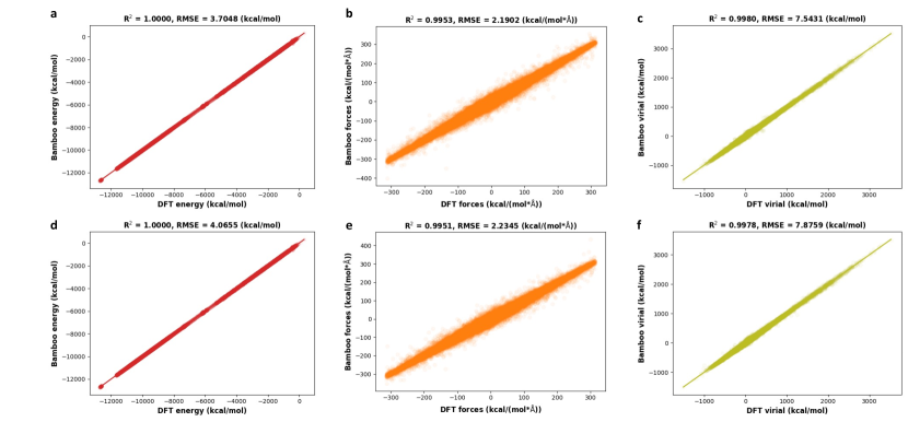
Figure S3: Fitting performance of BAMBOO before and after ensemble knowledge distillation and density calibration. a, b, c. DFT computed energy, force, and virial versus BAMBOO predicted quantities before ensemble knowledge distillation and density calibration, respectively. d, e, f. DFT computed energy, force, and virial versus BAMBOO predicted quantities after ensemble knowledge distillation and density calibration, respectively. The results are based on the validation set.

Here, we build the neural networks in BAMBOO by PyTorch [85], and we use the AdamX optimizer [95] with the learning rate of $10^{-2}$. In the training process, weight decay is set to 0.001, while the learning rate decreases at a rate of 0.99. The batch size is 128 for both training and validating. The training process is composed of 750 training epochs. The model consists of 3 layers, with 32 radial basis functions for edges and an embedding dimension of 64 for nodes. It features 16 attention heads, employs a cutoff radius of 5.0Å for each message passing layer, and includes the MLP with two layers for predicting energy and charge. The loss weights $\alpha$’s in equation (44) are provided as the default in the open source codes at [84] and listed in Table S1.

Table S1: Table of loss weights.

Loss weights	$\alpha_{\text{energy}}^{\text{training}}$	$\alpha_{\text{force}}^{\text{training}}$	$\alpha_{\text{virial}}^{\text{training}}$	$\alpha_{\text{charge}}^{\text{training}}$	$\alpha_{\text{dipole}}^{\text{training}}$	$\alpha_{\text{Qeq}}$
Value	0.01	0.3	0.01	10.0	10.0	300.0

A.5 DFT Dataset Construction

In this work, we use 720,000 clusters with the DFT calculated energy, atomic forces, virial tensor, dipole moment, and partial charge (CHELPG) to train BAMBOO. The calculations are performed utilizing the B3LYP [96] functional alongside the def2-svpd [97] basis set, supplemented by density fitting techniques based on the def2-universal-jkfit auxiliary basis [98]. Throughout the computational process, the convergence threshold for the self-consistent field is set to $1.0\times 10^{-10}$ a.u., with a maximum allowance of 100 iterations. Here, we use the open-source GPU4PySCF package [99, 100] developed by ByteDance Inc. for the DFT calculations. Compared with QChem [101] on 32 CPUs, GPU4PySCF on a single V100 GPU can reduce cost by 97% in terms of computation time and 95% in terms of cost.

The procedure of collecting cluster structures is described below: first we take clusters in Ref. [38] as the starting point, which contains species including EC, PC, VC, FEC, DMC, EMC, DEC, PF${}_{6}^{-}$, and Li⁺. Then, we train five BAMBOO models by the DFT labels of the initial cluster structures calculated by GPU4PySCF, and run MD simulations using one randomly picked model at 300K for 1 ns with the NPT ensemble on pure solvents of EA, EP, EO, ACT, and Novec7000, and solutions with EC:DMC:EMC:VC:LiFSI = 3:3:1:1:1 and EC:DMC:LiFSI:LiTFSI = 10:10:1:1 by moles. In the first round of MD simulations, we observe that spurious reactions (mainly bond breaking) would occur in most simulations, which is expected as the initial structures do not cover the chemistry of the new species, especially FSI^- and TFSI^-. Then, we sample clusters from the MD trajectories until the first spurious reaction happens, and we use the following active learning scheme to sample clusters from the MD trajectories.

1. Instead of focusing on the uncertainty of the energy of the cluster as discussed in Ref. [38], our attention shifts to the uncertainty of predictions concerning atomic properties $\vec{f}_{i}$ and $q_{i}$. First, we employ five models to compute the standard deviation of predictions of charge $\sigma_{q}$ and magnitude of force $\sigma_{||\vec{f}||}$ on each atom. We then select all atoms for which $\sigma_{q}>0.015$ a.u. and $\sigma_{||\vec{f}||}>3$ kcal/(mol$\cdot$Å). For hydrogen atoms, we lower the criteria to $\sigma_{q}>0.01$ a.u. and $\sigma_{||\vec{f}||}>2$ kcal/(mol$\cdot$Å) as hydrogen is significantly lighter than other elements and typically exhibits smaller magnitudes of $q$ and $\vec{f}$.

2. When encountering uncertain atoms (expect Li⁺), we first determine the molecule/anion to which the uncertain atom belongs, and consider the molecule/anion as a cluster.

3. Next, we search for molecules, anions, and cations that have at least one atom within a 5Å radius of the uncertain atom. This search includes the molecule/anion to which the uncertain atom belongs. We consider all the neighboring molecules/anions/cations found in this search as a cluster. It’s worth noting that if multiple atoms within a single molecule are identified as uncertain, we perform the search for neighboring molecules only once to minimize redundancy.

4. We input clusters containing no more than 110 atoms into GPU4PySCF for labelling, and incorporate the newly labeled clusters and DFT labels into the dataset for training.

5. We repeat steps 1-4 iteratively. Once a system demonstrates stability without spurious reactions during the 1 ns MD simulation, we terminate the procedure for that particular system.

We achieve stable MD simulations for all the pure solvents within two iterations, and for solutions within three iterations. In Figure S4, we present the distribution of number of atoms in clusters and the number of molecules in the datasets. We observe two peaks in cluster sizes: one with fewer atoms corresponding to single molecules/anions, and another with more atoms representing the complete cluster within 5Å of the central uncertain atoms. Regarding the distribution of molecules, EC, Novec7000, VC, and DMC are the four most frequently sampled molecules. Among these, EC and DMC are the two main solvents of interest in this study, while VC and Novec7000 possess unique structural features compared to other molecules (such as a carbon-carbon double bond in VC and a high ratio of fluorination in Novec7000).

Figure S4: a and b Count of number of atoms in a cluster and number of molecules/ions in the dataset, respectively.

Appendix B Ensemble Knowledge Distillation for MLFF

B.1 Theory

As noted in Ref. [40], MLFFs often encounter instability in MD simulations, particularly when extrapolating to systems not seen in the training set. In Figure S5a, we illustrate that even if the ensemble of MLFFs is well-trained and behaves consistently and accurately within the interpolation domain, the inherent randomness of neural networks might lead to greater variability in out-of-domain inference compared with in-domain inference [62]. Consequently, the ensemble of MLFFs may exhibit significantly different behaviors within the extrapolation domain. In Figure S5b, we propose a method to constrain the behavior of different MLFFs within the extrapolation domain by training them on the mean predictions. This approach not only mitigates differences among the ensemble of MLFFs within the extrapolation domain but also reduces MLFF errors by minimizing random errors.

We illustrate the reduction of random errors by expressing the predicted energy in terms of the true energy (or other quantities such as force and virial tensor), systematic error, and random error.

$$E_{\text{pred}}^{\text{initial}}=E_{\text{true}}+\delta E_{\text{systematic}}^{\text{initial}}+\delta E_{\text{random}}^{\text{initial}},$$ (45)

where $\delta E$ denotes the error of energy. We can write the mean of the predicted energy as:

$$\overline{E_{\text{pred}}^{\text{initial}}}=E_{\text{true}}+\overline{\delta E_{\text{systematic}}^{\text{initial}}}+\overline{\delta E_{\text{random}}^{\text{initial}}}.$$ (46)

According to the law of large number, if the mean is taken over sufficient amount of predictions, then we have $\overline{\delta E_{\text{systematic}}^{\text{initial}}}\approx\delta E_{\text{systematic}}^{\text{initial}}$ and $\overline{\delta E_{\text{random}}^{\text{initial}}}\approx 0$. Therefore, we have:

$$\overline{E_{\text{pred}}^{\text{initial}}}\approx E_{\text{true}}+\delta E_{\text{systematic}}^{\text{initial}},$$ (47)

which implies

$$|\overline{E_{\text{pred}}^{\text{initial}}}-E_{\text{true}}|<|E_{\text{pred}}^{\text{initial}}-E_{\text{true}}|.$$ (48)

In ensemble knowledge distillation, since we use $\overline{E_{\text{pred}}^{\text{initial}}}$ as the label to train the MLFF, we can write the predicted energy after ensemble knowledge distillation as:

$$\begin{split}E_{\text{pred}}^{\text{distilled}}&=\overline{E_{\text{pred}}^{\text{initial}}}+\delta E_{\text{systematic}}^{\text{distill}}+\delta E_{\text{random}}^{\text{distill}}\\ &\approx E_{\text{true}}+\delta E_{\text{systematic}}^{\text{initial}}+\delta E_{\text{systematic}}^{\text{distill}}+\delta E_{\text{random}}^{\text{distill}}.\\ \end{split}$$ (49)

Therefore, if we properly design the training process in ensemble knowledge distillation to minimize $\delta E_{\text{systematic}}^{\text{distill}}$ and $\delta E_{\text{random}}^{\text{distill}}$, we will achieve smaller difference between $E_{\text{true}}$ and $E_{\text{pred}}^{\text{distilled}}$ than $E_{\text{pred}}^{\text{initial}}$. In the case study of solid phase transformation, we will demonstrate that following ensemble knowledge distillation, the prediction error decreases.

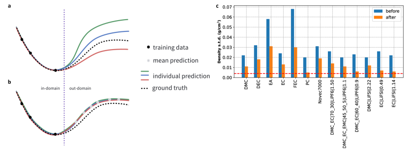
Figure S5: a and b Illustration of the interpolation and extrapolation behaviors before and after ensemble knowledge distillation, respectively. c Standard deviations of density from MD by five MLFFs before and after ensemble knowledge distillation.

B.2 Case Study of Liquid Electrolytes

In this study, as we train MLFFs using DFT data of small gas-phase clusters and utilize them to predict properties of large bulk liquid electrolytes, we essentially task MLFFs with extrapolation, which may introduce significant random noise into MD simulations. Hence, we adopt the following procedure to conduct ensemble knowledge distillation for liquid electrolytes:

1. Initially, we train five models purely by DFT data at random.

2. Subsequently, we randomly select one model to run 600 ps NPT MD simulations and 400 ps NVT MD simulations for all systems shown in Figure S5c.

3. With the trajectories obtained from the MD simulations from the previous step, we employ all five models to predict the energy, forces, and virial tensor of 100 randomly selected frames from the trajectory of each system.

4. Finally, we use the mean predictions as the labels to finetune the randomly selected model by the following loss function:

$$\begin{split}L_{\text{distill}}=L_{\text{training}}+\frac{1}{N_{\text{frame}}}\sum_{k}^{N_{\text{frame}}}\sum_{i}^{N_{\text{atom}}}&\alpha_{\text{energy}}^{\text{distill}}(\overline{E_{k}^{\text{BAMBOO}}}-E_{k}^{\text{BAMBOO}})^{2}\\ &+\frac{1}{N_{\text{atom}}}\alpha_{\text{force}}^{\text{distill}}||\overline{\vec{f}_{ki}^{\text{BAMBOO}}}-\vec{f}_{ki}^{\text{BAMBOO}}||^{2}\\ &+\alpha_{\text{virial}}^{\text{distill}}||\overline{\textbf{T}_{k}^{\text{BAMBOO}}}-\textbf{T}_{k}^{\text{BAMBOO}}||^{2}.\end{split}$$ (50)

Here, we incorporate $L_{\text{training}}$ into $L_{\text{distill}}$ to regulate the behavior of the distilled MLFF on DFT data. Specifically, in this study, we only fine-tune the weights of $\text{MLP}^{\text{energy}}$ of the MLFF, and we solely include the energy, forces, and virial terms in $L_{\text{training}}$ within equation (50). This approach is adopted because we do not include $L_{\text{Qeq}}$ in $L_{\text{distill}}$, as it is challenging to compute $\partial E^{\text{elec}}/\partial r_{i}$ for periodic bulk systems. Consequently, we refrain from adjusting weights that would impact the prediction of charge to maintain the constraint of charge equilibrium introduced during the initial training.

It is important to note that, to compare the effect of ensemble distillation on reducing standard deviations of MD results from different models in Figure S5c, we conduct distillation on all five models to calculate standard deviations from the five models. However, in the density alignment section below, we utilize only the randomly selected model to minimize computational costs.

As a result of ensemble knowledge distillation, we observe that the errors of predictions on DFT data remain almost unchanged (when $L_{\text{training}}$ is not included in $L_{\text{distill}}$, the increase in error can be up to 30%). Additionally, we find that the deviation between predictions of the randomly selected model and ensemble mean predictions is nearly halved. For systems with 4,000 atoms, the root mean square error (RMSE) between $\overline{E_{k}^{\text{BAMBOO}}}$ and $E_{k}^{\text{BAMBOO}}$ decreases from approximately 0.41 kcal/mol/atom to 0.23 kcal/mol/atom, RMSE of forces decreases from 1.22 kcal/mol/Å to 0.67 kcal/mol/Å, and RMSE of the virial tensor decreases from 164 kcal/mol to 87 kcal/mol. Detailed information about the training process of ensemble knowledge distillation is provided in the open-source code [84]. In Figure 2e in the main text and Figure S5c, we demonstrate that ensemble knowledge distillation can significantly reduce the variation of density from MD simulations by almost 50%. This illustrates the efficacy of ensemble knowledge distillation in improving the stability of MD results in liquids.

B.3 Case Study of Solid Phase Transformation

Figure S6: a and b structures of Li₄MoS₄ before and after the solid phase transformation (separation of the Mo rich phase and the Li rich phase), respectively. Green: Li, yellow: S, purple: Mo.

To demonstrate the broad applicability of ensemble knowledge distillation in improving the prediction performance and stability of MLFFs, we present another case study focusing on solid-phase transformation. Specifically, we investigate the system of Li₄MoS₄, a composition similar to Li₄Mo_0.5Ti_0.5S₄, which is a potential cathode material for lithium-ion batteries [102]. In this study, we explore the distribution of Mo atoms within the system. As depicted in Figure S6a, we begin by substituting Ti atoms in the crystal structure of Li₄TiS₄ (mp-766540 in the Materials Project database [103], with the space group of Pnma) with Mo to create the Li₄MoS₄ phase with evenly distributed Mo atoms. We subsequently optimize the crystal structure and conduct 50 ps NPT ab-initio molecular dynamics (AIMD) simulations on the initial structure. As shown in Table S3, our results indicate that while the Mo atoms remain evenly distributed at 700 K, they begin to accumulate in the upper-left corner of the simulation box at 800 K and 900 K, as illustrated in Figure S6b. This accumulation suggests a phase transformation, specifically a phase separation between the Mo-rich phase and the Li-rich phase, during the AIMD simulations at 800 K and 900 K. The different behaviors at different temperatures might be related to the energy barrier associated with the phase transformation: the energy barrier might have the magnitude such that the thermal fluctuation at 700 K is hard to push the system through the barrier during the 50 ps MD simulation, while the thermal fluctuations at 800 K and 900 K are large enough to activate the system over the energy barrier.

In this case study, our objective is to utilize MLFFs to replicate the phase transformation and demonstrate how ensemble knowledge distillation can enhance the stability of reproducing the phase transformation. For this purpose, we select M3GNet, the first and one of the most widely used pretrained universal MLFFs for solids [27]. We perform 20 ps NPT AIMD simulations with a time step of 1 fs at 300 K, 1000 K, and 10 ps at 2000 K. The initial structure for all MD simulations consists of a 2$\times$2$\times$1 supercell of crystalline Li₄MoS₄ with one random Li vacancy (totaling 143 atoms). Geometry optimization and AIMD are conducted using the Quantum Espresso package [104] with the PBE functional [105]. We utilize the first 10 ps trajectories of AIMD at 300 K and 1000 K as the training data to fine-tune the pretrained M3GNet, while the remaining 10 ps trajectories at 300 K, 1000 K, and 2000 K are used as the validation set. Employing stratified sampling with a frequency of 10 fs, we collect forces from a total of 2000 frames in AIMD trajectories as training data and 3000 frames as validation data. We optimize the pretrained M3GNet using 30 epochs with default hyperparameters as provided in the open-source codes of M3GNet [27]. Here, we fine-tune the pretrained M3GNet with 10 different random seeds to form an ensemble of M3GNets. Using this ensemble, we predict forces for the 3000 frames in the validation set and further fine-tune the 10 M3GNets in the ensemble using the mean predicted forces of the validation set in conjunction with the DFT forces of the training set. Finally, we employ all M3GNets to conduct 500 ps NPT MD simulations to observe whether phase transformation occurs. Since the Mo atoms in the initial structure are separated by 5.9 Å from each other, we classify whether phase separation occurs by examining whether there is a pair of Mo atoms within 3 Å of each other in the last frame of the simulation.

In Table S2, the data presented includes the average force error for the initial M3GNets, the distilled M3GNets’ average force error, and the force error from the mean predictions of the initial M3GNet ensemble in comparison with DFT across the validation set frames. It is evident that across all three temperatures, the distilled M3GNets exhibit a reduced average error compared to the initial M3GNets, yet this error exceeds that of the ensemble’s mean predictions. This finding aligns with our prior analysis, suggesting that by diminishing $\delta_{\text{random}}^{\text{initial}}$ and minimizing $\delta_{\text{systematic}}^{\text{distill}}$ and $\delta_{\text{random}}^{\text{distill}}$ as in equation (49), we can achieve $||\overline{\vec{f}_{\text{pred}}^{\text{initial}}}-\vec{f}_{\text{true}}||<||\vec{f}_{\text{pred}}^{\text{distilled}}-\vec{f}_{\text{true}}||<||\vec{f}_{\text{pred}}^{\text{initial}}-\vec{f}_{\text{true}}||$. Moreover, the distilled M3GNets exhibit a significantly lower standard deviation in mean absolute error (MAE) compared to the initial M3GNets, indicating that employing ensemble knowledge distillation enhances the prediction error stability of M3GNets.

Table S3 illustrates that while both initial and distilled M3GNets reliably predict whether phase transformation will occur at 700K and 900K, there is a discrepancy at 800K. Here, 60% of the initial M3GNet models predict a phase transformation, whereas the remaining 40% do not. In contrast, post-ensemble knowledge distillation, 90% of the distilled M3GNets anticipate a phase transformation, underscoring that distilled M3GNets offer a more unified and reliable prediction in MD simulations. It is important to acknowledge the inherent randomness in MD simulations; theoretically, with infinite simulation duration, all M3GNets should predict phase transformation. However, given that MD simulations are typically constrained by time, the limited simulation time results in the observed variability in simulation outcomes as shown in Table S3. The presented case studies, encompassing both solid phase transformation and liquid electrolytes, demonstrate that ensemble knowledge distillation is an effective strategy for enhancing the reliability and consistency of MLFFs across different systems.

Table S2: Mean absolute error (MAE) of prediction of forces from M3GNets compared with DFT. Unit of force is eV/Å.

Temperature	300K	1000K	2000K
Average MAE of initial M3GNets	0.0749 $\pm$ 0.008	0.1339 $\pm$ 0.008	0.2149 $\pm$ 0.035
Average MAE of distilled M3GNets	0.0745 $\pm$ 2$\times 10^{-5}$	0.1309 $\pm$ 3$\times 10^{-5}$	0.2036 $\pm$ 0.0002
MAE of mean predictions of initial M3GNets	0.0740	0.1288	0.2031

Table S3: Behaviors observed from AIMD, initial MLFFs, and distilled MLFFs under different temperatures for the system of Li₄MoS₄. “Even” refers to the state where Mo atoms are evenly distributed, and “accumulated” the state where Mo atoms are accumulated in a small region of the simulation box.

Temperature	AIMD, 50 ps	10 initial MLFFs, 500 ps	10 distilled MLFFs, 500 ps
700K	Even	Even:Accumulated = 10:0	Even:Accumulated = 10:0
800K	Accumulated	Even:Accumulated = 4:6	Even:Accumulated = 1:9
900K	Accumulated	Even:Accumulated = 0:10	Even:Accumulated = 0:10

Appendix C Density Alignment

C.1 Theory

In this work, we propose a physics-inspired approach to align the density predictions from MD simulations to experimentally measured density of liquids. The alignment is based on the isothermal compressibility of liquids:

$$\beta=\frac{1}{\rho}(\frac{d\rho}{dP})_{T},$$ (51)

where $\beta$ is the isothermal compressibility of a given liquid, $\rho$ is the density of the liquid, and $P$ is the pressure of the system. If we assume $\beta$ of a condensed liquid does not depend on $P$ when $P$ is not extremely high, which is a reasonable assumption in thermodynamics [106], then we have:

$$\Delta\ln(\rho)=\beta\Delta P.$$ (52)

Equation (52) suggests a linear correlation between $\Delta\ln(\rho)$ and $\Delta P$. This relationship is substantiated in Figure S7a-m, where the linearity holds across all examined liquids in the density alignment, evidenced by R² scores equal to or exceeding 0.98. This linear correlation implies that knowing the experimental density of a liquid and its corresponding density from an MD simulation allows us to determine the $\Delta\ln(\rho)$ between the two. Consequently, we can ascertain the $\Delta P$ required to adjust in the MD simulation to align the densities with experimental observations. Moreover, pressure in MD simulation is related to forces:

$$P=\frac{N_{\text{atoms}}k_{B}T}{V}+\frac{1}{3V}\sum_{i}^{N_{\text{atoms}}}\sum_{j}^{N_{\text{atoms}}}\langle\vec{f}_{ij},\vec{r}_{ij}\rangle,$$ (53)

where $k_{B}$ is the Boltzmann constant, $T$ is the temperature, and $V$ is the volume of the simulation box. Therefore, we find a bridge between the macroscopic observable density $\rho$ and microscopic quantity pairwise forces $\vec{f}_{ij}$:

$$\begin{split}\Delta\ln(\rho)&=\beta\Delta P=\beta(\Delta(\frac{N_{\text{atoms}}k_{B}T}{V})+\Delta(\frac{1}{3V}\sum_{i}^{N_{\text{atoms}}}\sum_{j}^{N_{\text{atoms}}}\langle\vec{f}_{ij},\vec{r}_{ij}\rangle)).\end{split}$$ (54)

Since $\vec{f}_{ij}$ is predicted by neural networks, equation (54) provides a way to calculate the derivative of density to weights of neural networks, which enables us to align BAMBOO with experimentally measured density.

Figure S7: a to m $\Delta$ln(density) versus $\Delta P$ of the 7 molecular liquids and 6 solutions included in density alignment, respectively. n Compressibility $\beta$ derived from the linear relation versus weight of salts.

C.2 Performance

As illustrated in Figure 1a, we employ the ensemble distilled model as the foundational base model for performing density alignment. This alignment process encompasses 7 molecular liquids and 6 solutions, including 3 with LiPF₆ and 3 with LiFSI. To initiate the alignment, we first calculate the coefficient $\beta$ for each liquid. This is achieved by training the distilled BAMBOO to adapt to various $\Delta P$s, utilizing the subsequent loss function:

$$\begin{split}L_{\text{align}}=L_{\text{training}}+\frac{1}{N_{\text{frame}}}\sum_{k}^{N_{\text{frame}}}&(\Delta P-\frac{1}{3V}\sum_{i}^{N_{\text{atoms}}}\sum_{j}^{N_{\text{atoms}}}\langle\vec{f}_{ij}^{\text{ align}}-\vec{f}_{ij}^{\text{ distill}},\vec{r}_{ij}\rangle)^{2}\\ &+(\alpha_{\text{energy}}^{\text{align}}(E_{k}^{\text{align}}-E_{k}^{\text{distill}})^{2})\\ &+\sum_{i}^{N_{\text{atoms}}}\alpha_{\text{force}}^{\text{align}}||\vec{f}_{ki}^{\text{align}}-\vec{f}_{ki}^{\text{distill}}||^{2}\\ &+\alpha_{\text{virial}}^{\text{align}}||\textbf{T}_{k}^{\text{align}}-\textbf{T}_{k}^{\text{distill}}||^{2}.\end{split}$$ (55)

Here, $\Delta P$ is the assigned pressure change as in the x-axes in Figure S7a-m, $\sum_{i}^{N_{\text{atoms}}}\sum_{j}^{N_{\text{atoms}}}\langle\vec{f}_{ij}^{\text{ align}}-\vec{f}_{ij}^{\text{ distill}},\vec{r}_{ij}\rangle/(3V)$ is the pressure change of aligned MLFF compared with the base MLFF (we omit the $\Delta(N_{\text{atoms}}k_{B}T/V)$ term in equation (54) as here we change pressure of the same frames without volume change, and the temperature change should also be negligible if $N_{\text{frame}}$ is large enough). We also include the terms of $(E_{k}^{\text{align}}-E_{k}^{\text{distill}})^{2}$, $||\vec{f}_{ki}^{\text{align}}-\vec{f}_{ki}^{\text{distill}}||^{2}$, $||\textbf{T}_{k}^{\text{align}}-\textbf{T}_{k}^{\text{distill}}||^{2}$, and $L_{\text{training}}$ to ensure that the aligned model would not drastically deviate from the initially trained model and the distilled model. In this work, we reuse the frames generated during the ensemble knowledge distillation for the alignment process as follows.

1. In the first round of alignment, we apply a uniform $\Delta P$ to each liquid for every model. This approach mirrors the ensemble knowledge distillation methodology, where we specifically adjust the weights of $\text{MLP}^{\text{energy}}$ within the MLFF for optimization. To enhance numerical stability, our focus is solely on the pressure changes stemming from inter-molecular interactions. Consequently, in equation (55), we only include $\langle\vec{f}_{ij}^{\text{align}}-\vec{f}_{ij}^{\text{distill}},\vec{r}_{ij}\rangle$, where atoms $i$ and $j$ do not belong to the same molecule or anion.

2. Following the initial alignment phase, we obtain a collection of aligned MLFFs, each corresponding to a distinct $\Delta P$. Utilizing these varied aligned MLFFs, we conduct 600 ps NPT simulations to gather the resulting densities ($\rho$). Consequently, as depicted in Figure S7a-m, we establish a linear correlation between $\Delta\ln(\rho)$ and the assigned $\Delta P$ for each liquid. Leveraging this linearity, we can determine the $\beta$ value for each liquid. This enables us to identify the specific $\Delta P$ that should be incorporated into the base MLFF for each liquid to align the $\Delta\ln(\rho)$ accurately.

3. In the final step, we employ the loss function specified in equation (55), applying the unique $\Delta P$ identified for each liquid, to align the base MLFF with experimental data. This process fine-tunes the MLFF to ensure that its predictions for density closely match the experimental observations, thus enhancing the accuracy and reliability of the model’s simulations in reflecting real-world phenomena.

In Figure S7n, we delve into the examination of the $\beta$ values derived from the linear relationships. It’s observed that molecules with similar structures exhibit comparable $\beta$ values. For instance, cyclic carbonates like EC, PC, and FEC share similar $\beta$s, as do linear molecules such as DMC, DEC, and EA. Generally, there is a trend where higher viscosity correlates with lower compressibility, aligning with the intuition that liquids more resistant to shear stress are also more resistant to compression [107]. Additionally, an increase in salt concentration leads to a decrease in $\beta$. For instance, in the case of EC and its solutions with LiFSI at different concentrations, there is a clear linear relationship with an R² score of 0.998, corroborating the empirical law that a solution’s compressibility linearly decreases with an increase in salt molality (more salts result in less compressibility) [108]. The consistent compressibility trends, as deduced from density alignment, further confirm the validity of the density alignment approach.

Upon completing the second round of density alignment, the final MLFF is established. Figure S3 illustrates a slight decrease in the model’s predictive accuracy for energy, forces, and virial compared with DFT calculations post-density alignment. Specifically, there is an 8% increase in the root mean square error (RMSE) for energy predictions, a 1% rise in forces RMSE, and a 4% uptick in virial RMSE. Despite these increases, the adjustments are made to enhance the model’s accuracy in density predictions, which can be critical for certain applications. Detailed documentation of the training process for density alignment is accessible in the publicly available source code [84].

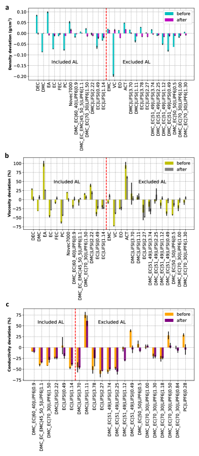
Figure S8: a to c Density, viscosity, and conductivity of molecular liquid and solutions before and after density alignment, respectively.

Figures S8 and 2 highlight the significant impact of density alignment on the physical properties of density, viscosity, and conductivity. The alignment process notably reduces the density error from 0.05 g/cm³ to approximately 0.01 g/cm³ for both the systems included in the alignment and those not directly aligned. This improvement suggests that density alignment, which adjusts the strength of inter-molecular interactions, has a degree of transferability to molecules with similar structures or solutions with varying salt concentrations not explicitly included in the alignment. For example, before alignment, cyclic carbonates like EC, FEC, and PC exhibit densities lower than experimental values. The alignment process increases inter-molecular interaction strength, thereby raising the predicted densities. Consequently, VC, another cyclic carbonate not included in the alignment, also shows an improved density prediction due to enhanced inter-molecular interactions among cyclic carbonates.

The effect of density alignment extends to solutions with EC and DMC as solvents and varying amounts of LiFSI salt. Prior to alignment, the MLFF tends to underestimate the densities of pure EC and DMC solvents. For aligned solutions at different molalities (0.49, 1.14, and 2.22 mol/kg), a pattern emerges: higher molality correlates with a lesser extent of density underestimation. This indicates that, initially, the MLFF underestimates solvent-solvent interactions while overestimating solvent-ion and/or ion-ion interactions. Through density alignment, these interactions are recalibrated—strengthening solvent-solvent and weakening solvent-ion/ion-ion interactions—leading to more accurate density predictions. Thus, for solutions with even higher molalities (3.70, 3.74, and 3.78 mol/kg) not included in the alignment, where the pre-alignment MLFF overestimated densities, the post-alignment MLFF, with adjusted interaction strengths, offers more accurate density predictions.

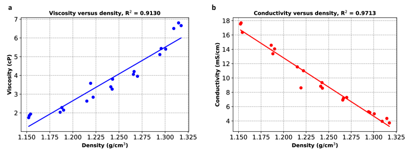
Figure S9: a and b Density versus viscosity, and density versus conductivity for the system of DMC$\_$EC$|$70$\_$30$|$LiPF6$|$1.0, respectively. The models leading to different densities are from the first round of density alignment.

In Figure S9, the observed strong dependence of viscosity and ionic conductivity on density aligns with expectations: a denser liquid typically exhibits stronger inter-molecular interactions, resulting in higher viscosity and lower conductivity. Thus, a post-alignment increase in density generally leads to a corresponding increase in viscosity and a decrease in conductivity. Figure S8b and c confirm this relationship for most liquids post-alignment. From Figure S8b and Figure 2g, it’s evident that the discrepancy in viscosity between MLFF MD simulations and experimental observations narrows significantly—from a 32% to a 17% deviation post-alignment. This improvement in viscosity accuracy is also seen in liquids not in the alignment, indicating the transferability of the alignment’s effects.

However, the situation is more complex with ionic conductivity. In certain cases, aligning MD density to experimental data inadvertently moves the ionic conductivity further from the experimental values. For instance, the systems EC$|$LiFSI$|$0.49 and DMC_EC$|$0.51_0.49$|$LiFSI$|$1.12 show underestimations in density and viscosity but have conductivities close to experimental values before alignment. Post-alignment, while their densities and viscosities adjust closer to experimental figures, their conductivities decrease, diverging from the experimental data. Consequently, the overall deviation in ionic conductivity decreases only modestly from 31% to 26% after density alignment. This suggests that while density alignment effectively narrows the gap in density and viscosity predictions, a more targeted alignment strategy might be needed to align ionic conductivity predictions more closely with experimental results.

Appendix D Ablation Study of Model Architecture

In this section, we provide the detailed results of the ablation study in Table S4, and description of the variants of GET (GIT, GE, and GET-no-charge). For GIT, we simply replace the equivariant relative vector $r_{ij}=(x_{ij},y_{ij},z_{ij})$ with an invariant feature $((||r_{ij}||,||r_{ij}||,||r_{ij}||)$, which keeps the model architecture. For GE, we skip the transformer architecture as in equation (9) and equation (10), and compute $y_{i}^{n}$ as below:

$$y_{i}^{n}=\sum_{j}v_{j}^{n}\odot d_{ij}.$$ (56)

In the process of modifying the GET model, when the transformer aspect in the GE is omitted, the dimension of $x_{i}^{n}$ within GE is increased from 64 to 76. This adjustment is made to ensure that GE and GET have a comparable number of parameters, thus maintaining a level of parity between the two in terms of model complexity. Regarding the GET-no-charge variant, all components associated with the charge $q_{i}$ are eliminated. This includes removing the MLPs that interact with $q_{i}$. To compensate for the reduction in complexity and to maintain a similar parameter count as the original GET, the number of layers in the $\text{MLP}^{\text{energy}}$ is increased from 2 to 4. These adjustments ensure that the GET-no-charge model retains a comparable level of complexity and parameter count to the standard GET, even in the absence of charge-related operations.

As shown in Table S4, GET exhibits superior predictive efficacy for both energy and forces derived from DFT when compared with GE and GIT. This observation intimates that equivariance might play a pivotal role, surpassing that of the transformer, as evidenced by GE’s reduced error margins relative to GIT. In the case of GET-no-charge, a significantly elevated error in forecasting DFT energy is noted in comparison to GET. This discrepancy can be ascribed to the intrinsic long-range dependence characteristic of electrostatic energy, which is inversely proportional to distance ($1/r$), coupled with the relatively diminished capacity of GNN to encapsulate long-range interactions as opposed to short-range dynamics [52]. Pertaining to the prediction of forces, GET-no-charge registers a marginally lower error than GET. This anomaly could potentially be attributed to the inherent limitations associated with the CHELPG method of labelling partial charges [94]. While electrostatic force exhibits lower sensitivity to long-range information compared with energy ($1/r^{2}$ for force and $1/r$ for energy), CHELPG is calibrated against the electrostatic potential at a considerable distance away from the cluster. Consequently, CHELPG is not optimally designed to capture short-range electrostatic forces. The employment of CHELPG for computing short-range electrostatic forces may inadvertently introduce non-physical biases into the neural network (NN)-facilitated force learning process, thereby exacerbating the learning challenge for the NN with an increase in error. This finding underscores the imperative for the development of more advanced abstract representations of electron density that can accurately and efficiently compute electrostatic forces. Finally, GET is distinguished by its minimal error in modeling density from MD simulations in contrast to GE, GIT, and GET-no-charge, a testament to its overarching superior capability in the precise prediction of DFT-calculated quantities.

Table S4: Results of ablation study of models trained on DFT data without ensemble knowledge distillation and density alignment. Here, “number of parameters” is the total number of degree of freedom of each MLFF that can be optimized in the training. “Density MAE” is based on the 13 systems included in density alignment as in Figure S8.

	GET	GIT	GE	GET no charge
Number of parameters	103,620	103,620	108,900	107,649
Energy RMSE (kcal/mol)	3.70 $\pm$ 0.04	4.19 $\pm$ 0.02	3.96 $\pm$ 0.03	10.67 $\pm$ 0.04
Forces RMSE (kcal/mol/Å)	2.19 $\pm$ 0.02	2.96 $\pm$ 0.02	2.32 $\pm$ 0.01	2.01 $\pm$ 0.02
Virial RMSE (kcal/mol)	7.54 $\pm$ 0.05	9.41 $\pm$ 0.09	7.95 $\pm$ 0.05	7.69 $\pm$ 0.09
Density MAE before distillation (g/cm3)	0.049 $\pm$ 0.007	0.114 $\pm$ 0.028	0.065 $\pm$ 0.020	0.082 $\pm$ 0.033

Appendix E Details of Molecular Dynamics

We employ LAMMPS [53] to conduct the MD simulations for BAMBOO. For each system, an initial step involves energy minimization, which is constrained to a maximum of 1000 iterations and 100,000 evaluations. Following this, the liquid systems are subjected to equilibrium under the NPT ensemble for 1 ns, with a step size maintained at 1 fs. The density values presented in this paper represent the average measured during the final 50 ps of the NPT simulation. Subsequently, we carry out a 4 ns production run under the NVT ensemble to determine the viscosity, diffusivity, and ionic conductivity of the systems.

The viscosity ($\eta$) and diffisivity ($D$) of the pure solvents and various mixtures are computed from equilibrium simulations by applying an Einstein relation as described below:

$$\eta=\cfrac{V}{2k_{B}T}\lim_{t\to\infty}\cfrac{d}{dt}\Biggl{\langle}\biggl{(}\int_{t_{0}}^{t_{0}+t}dt^{\prime}P_{\alpha\beta}(t^{\prime})\biggr{)}^{2}\Biggr{\rangle}_{t_{0}},$$ (57)

$$D=\frac{1}{6N}\lim_{t\to\infty}\cfrac{d}{dt}\Biggl{\langle}|\vec{r}_{i,t+t_{0}}-\vec{r}_{i,t_{0}}|^{2}\Biggr{\rangle}_{i,t_{0}},$$ (58)

where $V$ and $T$ represent the volume and the temperature of the simulations. $P_{\alpha\beta}(t^{\prime})$ is the shear component of the stress tensor at the time step $t^{\prime}$. $N$ represents the number of ions or molecules at interest, and $\vec{r}_{i,t}$ the 3D coordinate of ion/molecule $i$ at time $t$, t₀ the starting time step, and $t$ the total number of time steps in the simulation trajectories used for viscosity or diffusivity analysis.

Following the calculation of diffusion coefficients, we calculate transference number using the following equation:

$$t_{+}=\cfrac{D_{+}}{D_{+}+D_{-}}.$$ (59)

Two approaches are used to calculate ionic conductivities, that are the Nernst-Einstein method and a method described by Mistry $et$ $al$ [70] that built on Stefan-Maxwell diffusivities. In this work, by default the ionic conductivity is calculated by Mistry $et$ $al$ [70] unless specified. The Nernst-Einstein equation is described below:

$$\sigma_{NE}=\cfrac{e^{2}}{Vk_{B}T}(N_{+}z^{2}_{+}\bar{D}_{+}+N_{-}z^{2}_{-}\bar{D}_{-}),$$ (60)

where $e$ is the elementary charge, $k_{B}$ the Boltzmann constant, and V and T are volume and temperature of the simulated system. $\bar{D}_{\pm}$, $z_{\pm}$, and $N_{\pm}$ are the self-diffusion coefficients, the charges, and the counts of the positive and negative ions, respectively.

In our calculations for the diffusion coefficients and conductivities, we apply finite size correction factor (FSC) to account for the effect of simulation box sizes [109]. The FSC is calculated using the following equation:

$$\text{FSC}=\cfrac{2.837298\times k_{B}\times T}{6\pi\eta L},$$ (61)

where $\eta$ is the estimated viscosity and $L$ is the simulation box length.

Appendix F More Solvation Structure Analyses

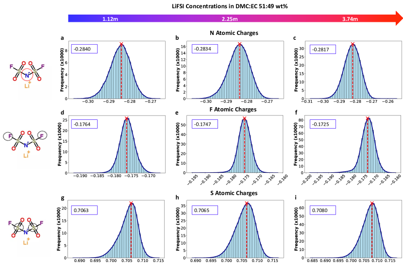
Figure S10: The atomic charge distributions of N, S, and F of the three simulated LiFSI electrolytes using BAMBOO MLFF. The electrolytes analyzed are the same systems as those shown in Figure 4 and F1-F3 electrolytes shown in Figure 3.

Figure S11: The cumulative coordination of solvent and anion species around Li⁺. a-c show the results of electrolytes 1.12m, 2.25m, and 3.74m LiFSI in DMC:EC 51:49 wt$\%$, respectively. The total coordination numbers for each simulated system is presented in each figure panel. The legends indicate the coordination is obtained by analyzing the atomise interactions between Li⁺ and the Os of surrounding solvents and anion molecules. The electrolytes analyzed are the same systems as those shown in Figure 4 and F1-F3 electrolytes shown in Figure 3.

The charge histograms shown in Figure 4 and Figure S10 are derived by first collecting atomic partial charges from each frame of a 4ns simulation, totalling 4,000 frames, followed by histogram analyses. The peaks corresponding to each normal distribution in the figure panels are identified using the find-peaks function as implemented in scipy.signal module. The solvation structures were determined by extracting Li clusters using MDAnalysis [110] with radius cut-off 2.2Å determined from Li-FSI radial distribution functions. This information can be read from the cumulative coordination around Li⁺ presented in Figure S11. The frames involved in the cluster extraction are in consistent with the charge histograms.

Appendix G Liquid Electrolyte Data

In this section, we show all the simulated and experimental properties of solvents and solutions for readers’ reference.

Table S5: The simulated densities in g/cm³ of pure solvents and mixtures that are used in the density alignment process. The salt concentrations (“m”) of mixtures are in molality, defined as the mole of salt in kilograms of solvent. The compositions of the LiFSI-containing mixtures are converted based on their molar ratios as used in the original literature. The electrolytes are presented in “solvents$|$solvent weight $\%$$|$salt$|$salt molality” format. The uncertainty associated with the density prediction ranges from 0.001-0.003 g/cm³. All simulations are performed at 298K, except for EC and FEC, which were conducted at 313K.

Mixtures	Compositions	BAMBOO	Expt	Expt. Ref.
DMC	DMC 100 wt%	1.060	1.06	[1]
DEC	DEC 100 wt%	0.969	0.97	[1]
PC	PC 100 wt%	1.188	1.20	[111]
EC	EC 100 wt%	1.310	1.32	[1]
FEC	FEC 100 wt%	1.474	1.48	[64]
EA	EA 100 wt%	0.892	0.90	[112]
Novec7000	Novec7000 100 wt%	1.416	1.41	[44]
P5	DMC_EC$|$60_40$|$LiPF6$|$0.9	1.236	1.239	Acquired from [68]
P6	DMC_EC_EMC$|$45_50_5$|$LiPF6$|$1.1	1.274	1.273	Acquired from [68]
P7	DMC_EC$|$70_30$|$LiPF6$|$1.5	1.255	1.268	Acquired from [68]
F4	DMC$|$LiFSI$|$2.22	1.260	1.27	DMC:LiFSI 5:1[4]
F5	EC$|$LiFSI$|$0.49	1.359	1.38	EC:LiFSI 23:1 [4]
F6	EC$|$LiFSI$|$1.14	1.412	1.43	EC:LiFSI 10:1 [4]

Table S6: The simulated densities in g/cm³ of pure solvents and mixtures that are not used in the density alignment process. The salt concentrations (“m”) of mixtures are in molality, defined as the mole of salt in kilograms of solvent. The compositions of the LiFSI-containing mixtures are converted based on their molar ratios as used in the original literature. The electrolytes are presented in “solvents$|$solvent weight $\%$$|$salt$|$salt molality” format. The uncertainty associated with the density prediction ranges from 0.001-0.003 g/cm³. The simulations are conducted at 298K.

Mixtures	Compositions	BAMBOO	Expt	Expt. Ref.
EMC	EMC 100 wt%	1.015	1.0	[1]
VC	VC 100 wt %	1.370	1.355	[1]
EO	EO 100 wt %	0.769	0.79	[113]
ACT	ACT 100 wt %	0.808	0.79	[113]
S1	DMC_EC$|$70_30	1.131	1.13	SI of [68]
S2	DMC_EC$|$50_50	1.183	1.18	SI of [68]
S3	EMC_EC$|$70_30	1.100	1.095	SI of [68]
S4	EMC_EC$|$50_50	1.160	1.156	SI of [68]
P1	DMC_EC$|$50_50$|$LiPF6$|$0.5	1.224	1.23	Acquired from [68]
P4	DMC_EC$|$70_30$|$LiPF6$|$1.0	1.221	1.228	Acquired from [68]
P8	DMC_EC$|$70_30$|$LiPF6$|$1.3	1.243	1.252	Acquired from [68]
F7	DMC$|$LiFSI$|$3.70	1.361	1.36	DMC:LiFSI 3:1 [4]
F8	DMC$|$LiFSI$|$1.11	1.167	1.18	DMC:LiFSI 10:1 [4]
F9	EC$|$LiFSI$|$3.78	1.555	1.57	EC:LiFSI 3:1 [4]
F10	EC$|$LiFSI$|$2.27	1.484	1.50	EC:LiFSI 5:1 [4]
F3	DMC_EC$|$51_49$|$LiFSI$|$3.74	1.456	1.46	DMC:EC:LiFSI 3:3:2 [4]
F2	DMC_EC$|$51_49$|$LiFSI$|$2.25	1.372	1.38	DMC:EC:LiFSI 5:5:2 [4]
F1	DMC_EC$|$51_49$|$LiFSI$|$1.12	1.285	1.30	DMC:EC:LiFSI 10:10:2 [4]
F11	DMC_EC$|$51_49$|$LiFSI$|$0.49	1.229	1.24	DMC:EC:LiFSI 23:23:2 [4]

Table S7: The simulated viscosities in cP of solvents

Mixtures	Compositions	Temperature, K	BAMBOO	Expt
DMC	DMC 100 wt%	298	0.629$\pm$0.0290	0.585, 0.706 [1, 65]
DEC	DEC 100 wt%	298	0.766$\pm$0.0243	0.75 [1]
EMC	EMC 100 wt%	298	0.724$\pm$0.0204	0.65 [1]
VC	VC 100 wt%	298	1.104$\pm$0.0540	1.78 [114]
EC	EC 100 wt%	313	1.381$\pm$0.0386	1.60-1.90 [1, 64, 65]
FEC	FEC 100 wt%	313	2.349$\pm$0.0941	2.24-4.1 [64, 66, 65]
Novec7000	Novec7000 100 wt%	298	0.447$\pm$0.0211	0.45 [44]
EA	EA 100 wt%	298	0.542$\pm$0.0071	0.43 [115]
PC	PC 100 wt%	298	1.426$\pm$0.0452	2.53 [1]
EO	EO 100 wt%	298	0.829$\pm$0.0500	1.1 [113]
ACT	ACT 100 wt%	298	0.502$\pm$0.0101	0.31 [113]
S1	DMC_EC$|$70_30	293	0.720$\pm$0.0136	0.95 [69]
S1	DMC_EC$|$70_30	300	0.673$\pm$0.0171	NA
S1	DMC_EC$|$70_30	303	0.644$\pm$0.0197	0.83 [69]
S1	DMC_EC$|$70_30	313	0.602$\pm$0.0129	0.73 [69]
S3	EMC_EC$|$70_30	293	0.842$\pm$0.0126	1.11 [69]
S3	EMC_EC$|$70_30	300	0.820$\pm$0.0163	NA
S3	EMC_EC$|$70_30	303	0.835$\pm$0.0253	0.97 [69]
S3	EMC_EC$|$70_30	313	0.734$\pm$0.0161	0.87 [69]

Table S8: The simulated viscosities ($\eta$), conductivities ($\sigma$) of cation of LiFSI and LiPF₆ based electrolytes at 298K. The uncertainty for the conductivities calculated using Mistry’s method ranges from 0.35 to 1.38 mS/cm, while the values calculated using NE method ranges from 0.11 to 2.20 mS/cm. The uncertainty for the predicted viscosity for medium and low concentrated electrolytes (P1-P9, and F1, F5-6, F8, F11) are below 0.1 cP, while the uncertainty for the remaining highly concentrated electrolytes are generally from 0.3 cP to 0.6 cP with the maximum of 3 cP for F9, respectively. The viscosity values for the carbonate based electrolytes are acquired from authors of ref[68] by private communications.

Mixtures	Compositions	$\eta_{\text{simu}}$	$\eta_{\text{Expt}}$	$\sigma_{\text{Mistry}}$	$\sigma_{\text{NE}}$	$\sigma_{\text{Expt}}$
P1	DMC_EC$|$50_50$|$LiPF6$|$0.5	1.891	2.219 [68]	11.201	12.420	12.14 [68]
P2	DMC_EC$|$70_30$|$LiPF6$|$0.5	1.656	NA	11.361	13.133	10.89 [68]
P3	DMC_EC$|$70_30$|$LiPF6$|$0.84	2.413	NA	11.990	15.106	12.91 [68]
P4	DMC_EC$|$70_30$|$LiPF6$|$1.0	2.683	2.734 [68]	12.881	15.451	12.43 [68]
P5	DMC_EC$|$60_40$|$LiPF6$|$0.9	2.847	2.778 [68]	11.531	14.860	12.793 [68]
P6	DMC_EC_EMC$|$45_50_5$|$LiPF6$|$1.1	4.716	4.566 [68]	8.021	10.669	12.175 [68]
P7	DMC_EC$|$70_30$|$LiPF6$|$1.5	4.810	4.472 [68]	8.713	12.241	12.144 [68]
P8	DMC_EC$|$70_30$|$LiPF6$|$1.3	3.984	3.767 [68]	9.573	13.171	12.118 [68]
P9	PC$|$LiPF6$|$0.28	2.517	NA	4.735	4.053	4.967 [116]
F1	DMC_EC$|$51_49$|$LiFSI$|$1.12	3.548	3.4 [4]	9.828	13.069	14 [4]
F2	DMC_EC$|$51_49$|$LiFSI$|$2.25	11.121	9.8 [4]	4.369	6.592	9.8 [4]
F3	DMC_EC$|$51_49$|$LiFSI$|$3.74	24.946	36.9 [4]	2.266	3.527	4.5 [4]
F4	DMC$|$LiFSI$|$2.22	4.653	3.9 [4]	9.237	13.142	12.2 [4]
F5	EC$|$LiFSI$|$0.49	3.184	4.1 [4]	7.013	8.099	8.7 [4]
F6	EC$|$LiFSI$|$1.14	6.179	8.1 [4]	5.907	7.672	9.7 [4]
F7	DMC$|$LiFSI$|$3.70	13.304	12.9 [4]	4.363	6.739	8.1 [4]
F8	DMC$|$LiFSI$|$1.11	1.629	1.5 [4]	15.984	20.209	9.9 [4]
F9	EC$|$LiFSI$|$3.78	34.183	NA	1.738	2.472	2.3 [4]
F10	EC$|$LiFSI$|$2.27	17.283	33.1 [4]	2.597	3.063	5.6 [4]
F11	DMC_EC$|$51_49$|$LiFSI$|$0.49	1.85	1.9 [4]	11.015	12.771	11.5 [4]

Table S9: The simulated diffusion coefficients ($10^{-10}$ m²/s) of cations and anions, and the calculated transference numbers in LiPF₆ and LiFSI-based electrolytes at 298K.

Mixtures	Compositions	D${}_{+,\text{self}}$	D${}_{-,\text{self}}$	t+
P1	DMC_EC$|$50_50$|$LiPF6$|$0.5	2.898	4.298	0.403$\pm$0.031
P2	DMC_EC$|$70_30$|$LiPF6$|$0.5	3.256	4.651	0.412$\pm$0.028
P3	DMC_EC$|$70_30$|$LiPF6$|$0.84	2.587	3.493	0.425$\pm$0.027
P4	DMC_EC$|$70_30$|$LiPF6$|$1.0	2.435	3.307	0.424$\pm$0.035
F1	DMC_EC$|$51_49$|$LiFSI$|$1.12	1.919	2.412	0.443$\pm$0.046
F2	DMC_EC$|$51_49$|$LiFSI$|$2.25	0.875	0.952	0.479$\pm$0.055
F3	DMC_EC$|$51_49$|$LiFSI$|$3.74	0.548	0.550	0.499$\pm$0.056

References

- [1] Kang Xu “Nonaqueous liquid electrolytes for lithium-based rechargeable batteries” In Chem. Rev. 104.10 ACS Publications, 2004, pp. 4303–4418
- [2] Kang Xu “Electrolytes, Interfaces and Interphases: Fundamentals and Applications in Batteries” Royal Society of Chemistry, 2023
- [3] Y Shirley Meng, Venkat Srinivasan and Kang Xu “Designing better electrolytes” In Science 378.6624 American Association for the Advancement of Science, 2022, pp. eabq3750
- [4] Jianhui Wang et al. “Superconcentrated electrolytes for a high-voltage lithium-ion battery” In Nat. Commun. 7.1 Nature Publishing Group UK London, 2016, pp. 12032
- [5] Corey M Efaw et al. “Localized high-concentration electrolytes get more localized through micelle-like structures” In Nat. Mater. 22.12 Nature Publishing Group UK London, 2023, pp. 1531–1539
- [6] Zhiao Yu et al. “Molecular design for electrolyte solvents enabling energy-dense and long-cycling lithium metal batteries” In Nat. Energy 5.7 Nature Publishing Group UK London, 2020, pp. 526–533
- [7] Chibueze V Amanchukwu et al. “A new class of ionically conducting fluorinated ether electrolytes with high electrochemical stability” In J. Am. Chem. Soc. 142.16 ACS Publications, 2020, pp. 7393–7403
- [8] Di Lu et al. “Ligand-channel-enabled ultrafast Li-ion conduction” In Nature Nature Publishing Group UK London, 2024, pp. 1–7
- [9] Kang Xu et al. “Solvation sheath of Li+ in nonaqueous electrolytes and its implication of graphite electrolyte interface chemistry” In J. Phys. Chem. C 111.20 ACS Publications, 2007, pp. 7411–7421
- [10] Oleg Borodin et al. “Uncharted waters: super-concentrated electrolytes” In Joule 4.1 Elsevier, 2020, pp. 69–100
- [11] Oliver T Unke et al. “Machine learning force fields” In Chem. Rev. 121.16 ACS Publications, 2021, pp. 10142–10186
- [12] Daan Frenkel and Berend Smit “Understanding molecular simulation: from algorithms to applications” Elsevier, 2023
- [13] Thomas A Halgren “Merck molecular force field. I. Basis, form, scope, parameterization, and performance of MMFF94” In J. Comput. Chem. 17.5-6 Wiley Online Library, 1996, pp. 490–519
- [14] Jörg Behler and Michele Parrinello “Generalized Neural-Network Representation of High-Dimensional Potential-Energy Surfaces” In Phys. Rev. Lett. 98 American Physical Society, 2007, pp. 146401 DOI: 10.1103/PhysRevLett.98.146401
- [15] Linfeng Zhang et al. “Deep Potential Molecular Dynamics: A Scalable Model with the Accuracy of Quantum Mechanics” In Phys. Rev. Lett. 120 American Physical Society, 2018, pp. 143001 DOI: 10.1103/PhysRevLett.120.143001
- [16] Yu Lysogorskiy et al. “Performant implementation of the atomic cluster expansion (PACE) and application to copper and silicon” In npj Comput. Mater. 7, 2021, pp. 97 DOI: 10.1038/s41524-021-00559-9
- [17] K.. Schütt et al. “SchNet – A deep learning architecture for molecules and materials” In J. Chem. Phys. 148.24, 2018, pp. 241722 DOI: 10.1063/1.5019779
- [18] Simon Batzner et al. “E(3)-equivariant graph neural networks for data-efficient and accurate interatomic potentials” In Nat. Commun. 13, 2022 DOI: 10.1038/s41467-022-29939-5
- [19] Yi-Lun Liao and Tess Smidt “Equiformer: Equivariant Graph Attention Transformer for 3D Atomistic Graphs”, 2023 arXiv:2206.11990 [cs.LG]
- [20] Philipp Thölke and Gianni De Fabritiis “TorchMD-NET: Equivariant Transformers for Neural Network based Molecular Potentials”, 2022 arXiv:2202.02541 [cs.LG]
- [21] Tsz Wai Ko, Jonas A Finkler, Stefan Goedecker and Jörg Behler “A fourth-generation high-dimensional neural network potential with accurate electrostatics including non-local charge transfer” In Nat. Commun. 12.1 Nature Publishing Group UK London, 2021, pp. 398
- [22] Linfeng Zhang et al. “A deep potential model with long-range electrostatic interactions” In J. Chem. Phys. 156.12, 2022, pp. 124107 DOI: 10.1063/5.0083669
- [23] Dylan Anstine, Roman Zubatyuk and Olexandr Isayev “AIMNet2: A Neural Network Potential to Meet your Neutral, Charged, Organic, and Elemental-Organic Needs”, 2023 DOI: 10.26434/chemrxiv-2023-296ch
- [24] Oliver Unke and Markus Meuwly “PhysNet: A Neural Network for Predicting Energies, Forces, Dipole Moments and Partial Charges” In J. Chem. Theory Comput. 15, 2019 DOI: 10.1021/acs.jctc.9b00181
- [25] Oliver Unke et al. “SpookyNet: Learning force fields with electronic degrees of freedom and nonlocal effects” In Nat. Commun. 12, 2021 DOI: 10.1038/s41467-021-27504-0
- [26] Hongyu Yu et al. “Spin-Dependent Graph Neural Network Potential for Magnetic Materials”, 2023 arXiv:2203.02853 [physics.comp-ph]
- [27] Chi Chen and Shyue Ong “A universal graph deep learning interatomic potential for the periodic table” In Nat. Comput. Sci. 2, 2022, pp. 718–728 DOI: 10.1038/s43588-022-00349-3
- [28] Bowen Deng et al. “CHGNet as a pretrained universal neural network potential for charge-informed atomistic modelling” In Nat. Mach. Intell. 5.9, 2023 DOI: 10.1038/s42256-023-00716-3
- [29] Amil Merchant et al. “Scaling deep learning for materials discovery” In Nature 624, 2023, pp. 1–6 DOI: 10.1038/s41586-023-06735-9
- [30] Duo Zhang et al. “DPA-2: Towards a universal large atomic model for molecular and material simulation”, 2023 arXiv:2312.15492 [physics.chem-ph]
- [31] Ilyes Batatia et al. “A foundation model for atomistic materials chemistry”, 2024 arXiv:2401.00096 [physics.chem-ph]
- [32] Dávid Péter Kovács et al. “MACE-OFF23: Transferable Machine Learning Force Fields for Organic Molecules”, 2023 arXiv:2312.15211 [physics.chem-ph]
- [33] Hao Wang and Weitao Yang “Force Field for Water Based on Neural Network” PMID: 29775313 In J. Phys. Chem. Lett. 9.12, 2018, pp. 3232–3240 DOI: 10.1021/acs.jpclett.8b01131
- [34] Junji Zhang, Joshua Pagotto, Tim Gould and Timothy T. Duignan “Accurate, fast and generalisable first principles simulation of aqueous lithium chloride”, 2023 arXiv:2310.12535 [physics.chem-ph]
- [35] Ioan B. Magdău et al. “Machine learning force fields for molecular liquids: Ethylene Carbonate/Ethyl Methyl Carbonate binary solvent” In npj Comput. Mater. 9, 2023, pp. 1–15
- [36] Hadrián Montes-Campos et al. “A Differentiable Neural-Network Force Field for Ionic Liquids” PMID: 34941253 In J. Chem. Inf. Model. 62.1, 2022, pp. 88–101 DOI: 10.1021/acs.jcim.1c01380
- [37] Feng Wang and Jun Cheng “Understanding the solvation structures of glyme-based electrolytes by machine learning molecular dynamics” In Chinese J. Struc. Chem. 42.9, 2023, pp. 100061 DOI: https://doi.org/10.1016/j.cjsc.2023.100061
- [38] Steven Dajnowicz et al. “High-Dimensional Neural Network Potential for Liquid Electrolyte Simulations” In J. Phys. Chem. B 126, 2022 DOI: 10.1021/acs.jpcb.2c03746
- [39] Leif Jacobson et al. “Transferable Neural Network Potential Energy Surfaces for Closed-Shell Organic Molecules: Extension to Ions” In J. Chem. Theory Comput. 18, 2022 DOI: 10.1021/acs.jctc.1c00821
- [40] Xiang Fu et al. “Forces are not enough: Benchmark and critical evaluation for machine learning force fields with molecular simulations” In arXiv preprint arXiv:2210.07237, 2022
- [41] Franco Ormeño and Ignacio General “Convergence and equilibrium in molecular dynamics simulations” In Commun. Chem. 7, 2024 DOI: 10.1038/s42004-024-01114-5
- [42] Xinyan Wang et al. “DMFF: An Open-Source Automatic Differentiable Platform for Molecular Force Field Development and Molecular Dynamics Simulation” PMID: 37589304 In J. Chem. Theory Comput. 19.17, 2023, pp. 5897–5909 DOI: 10.1021/acs.jctc.2c01297
- [43] Joe G. Greener and David T. Jones “Differentiable molecular simulation can learn all the parameters in a coarse-grained force field for proteins” In PLOS ONE 16.9 Public Library of Science, 2021, pp. 1–20 DOI: 10.1371/journal.pone.0256990
- [44] “3M™ Novec™ 7000 Engineered Fluid” URL: https://multimedia.3m.com/mws/media/121372O/3m-novec-7000-engineered-fluid-tds.pdf
- [45] Umar Asif, Jianbin Tang and Stefan Harrer “Ensemble knowledge distillation for learning improved and efficient networks” In arXiv preprint arXiv:1909.08097, 2019
- [46] David Chandler, John D. Weeks and Hans C. Andersen “Van der Waals Picture of Liquids, Solids, and Phase Transformations” In Science 220.4599, 1983, pp. 787–794 DOI: 10.1126/science.220.4599.787
- [47] Georgios M. Kontogeorgis, Bjørn Maribo-Mogensen and Kaj Thomsen “The Debye-Hückel theory and its importance in modeling electrolyte solutions” In Fluid Ph. Equilib. 462 Elsevier, 2018, pp. 130–152 DOI: 10.1016/j.fluid.2018.01.004
- [48] Pier Poier, Louis Lagardère, Jean-Philip Piquemal and Frank Jensen “Molecular Dynamics Using Nonvariational Polarizable Force Fields: Theory, Periodic Boundary Conditions Implementation, and Application to the Bond Capacity Model” In J. Chem. Theory Comput. 2019, 2019 DOI: 10.1021/acs.jctc.9b00721
- [49] Heiner Schröder, Anne Creon and Tobias Schwabe “Reformulation of the D3(Becke–Johnson) Dispersion Correction without Resorting to Higher than C6 Dispersion Coefficients” In J. Chem. Theory Comput. 11.7 American Chemical Society (ACS), 2015, pp. 3163–3170 DOI: 10.1021/acs.jctc.5b00400
- [50] Alejandro Torres-Sánchez, Juan M. Vanegas and Marino Arroyo “Geometric derivation of the microscopic stress: A covariant central force decomposition” Special Issue in honor of Michael Ortiz In J. Mech. Phys. Solids 93, 2016, pp. 224–239 DOI: https://doi.org/10.1016/j.jmps.2016.03.006
- [51] Ashish Vaswani et al. “Attention is all you need” In Advances in neural information processing systems 30, 2017
- [52] Sheng Gong et al. “Examining graph neural networks for crystal structures: Limitations and opportunities for capturing periodicity” In Sci. Adv. 9.45, 2023, pp. eadi3245 DOI: 10.1126/sciadv.adi3245
- [53] A.. Thompson et al. “LAMMPS - a flexible simulation tool for particle-based materials modeling at the atomic, meso, and continuum scales” In Comp. Phys. Comm. 271, 2022, pp. 108171 DOI: 10.1016/j.cpc.2021.108171
- [54] Albert Musaelian et al. “Learning local equivariant representations for large-scale atomistic dynamics” In Nat. Commun. 14.1 Nature Publishing Group UK London, 2023, pp. 579
- [55] Yusong Wang et al. “ViSNet: an equivariant geometry-enhanced graph neural network with vector-scalar interactive message passing for molecules” In arXiv preprint arXiv:2210.16518, 2022
- [56] Ilyes Batatia et al. “MACE: Higher order equivariant message passing neural networks for fast and accurate force fields” In Advances in Neural Information Processing Systems 35, 2022, pp. 11423–11436
- [57] Raul P. etal. “TorchMD-Net 2.0: Fast Neural Network Potentials for Molecular Simulations”, 2024 arXiv:2402.17660 [cs.LG]
- [58] Guillem Simeon and Gianni De Fabritiis “Tensornet: Cartesian tensor representations for efficient learning of molecular potentials” In Advances in Neural Information Processing Systems 36, 2024
- [59] Chao Lu et al. “OPLS4: Improving Force Field Accuracy on Challenging Regimes of Chemical Space” PMID: 34096718 In J. Chem. Theory Comput. 17.7, 2021, pp. 4291–4300 DOI: 10.1021/acs.jctc.1c00302
- [60] Oleg Borodin “Polarizable Force Field Development and Molecular Dynamics Simulations of Ionic Liquids” PMID: 19637900 In J. Phys. Chem. B 113.33, 2009, pp. 11463–11478 DOI: 10.1021/jp905220k
- [61] “Comparison of Simulation and Experiment” URL: https://wasatchmolecular.com/tables.pdf
- [62] Georg Martius and Christoph H Lampert “Extrapolation and learning equations” In arXiv preprint arXiv:1610.02995, 2016
- [63] Adarsh R. Dave “Automated Design and Discovery of Liquid Electrolytes for Lithium-Ion Batteries”, 2023 DOI: 10.1184/R1/22735025.v1
- [64] Kousuke Hagiyama et al. “Physical properties of substituted 1, 3-dioxolan-2-ones” In Chem. Lett. 37.2 Oxford University Press, 2008, pp. 210–211
- [65] Yukio Sasaki “Chapter 13 - Physical and electrochemical properties and application to lithium batteries of fluorinated organic solvents” In Fluorinated Materials for Energy Conversion Amsterdam: Elsevier Science, 2005, pp. 285–304 DOI: https://doi.org/10.1016/B978-008044472-7/50041-2
- [66] Alar Jänes, Thomas Thomberg, Jaanus Eskusson and Enn Lust “Fluoroethylene Carbonate and Propylene Carbonate Mixtures Based Electrolytes for Supercapacitors” In ECS Trans. 58.27 IOP Publishing, 2014, pp. 71
- [67] Heiner Jakob Gores et al. “Liquid nonaqueous electrolytes” In Handbook of battery materials Wiley Online Library, 2011, pp. 525–626
- [68] Adarsh Dave et al. “Autonomous optimization of non-aqueous Li-ion battery electrolytes via robotic experimentation and machine learning coupling” In Nat. Commun. 13.1 Nature Publishing Group UK London, 2022, pp. 5454
- [69] ER Logan et al. “A study of the transport properties of ethylene carbonate-free Li electrolytes” In J. Electrochem. Soc. 165.3 The Electrochemical Society, 2018, pp. A705–A716
- [70] Aashutosh Mistry, Zhou Yu, Lei Cheng and Venkat Srinivasan “On Relative Importance of Vehicular and Structural Motions in Defining Electrolyte Transport” In J. Electrochem. Soc. 170.11 IOP Publishing, 2023, pp. 110536
- [71] David S Hall et al. “Exploring classes of co-solvents for fast-charging lithium-ion cells” In J. Electrochem. Soc. 165.10 IOP Publishing, 2018, pp. A2365
- [72] Xiaowei Ma et al. “A study of highly conductive ester co-solvents in Li [Ni0. 5Mn0. 3Co0. 2] O2/Graphite pouch cells” In Electrochim. Acta. 270 Elsevier, 2018, pp. 215–223
- [73] Kang Xu “Navigating the minefield of battery literature” In Commun. Mater. 3.1 Nature Publishing Group UK London, 2022, pp. 31
- [74] Lifei Li et al. “Transport and electrochemical properties and spectral features of non-aqueous electrolytes containing LiFSI in linear carbonate solvents” In J. Electrochem. Soc. 158.2 IOP Publishing, 2010, pp. A74
- [75] Toshihiro Takekawa, Kazuhiro Kamiguchi, Hideto Imai and Masaharu Hatano “Physicochemical and electrochemical properties of the organic solvent electrolyte with lithium bis (fluorosulfonyl) imide (LiFSI) as lithium-ion conducting salt for lithium-ion batteries” In ECS Trans 64.24 IOP Publishing, 2015, pp. 11
- [76] Xingyu Chen, Fangfang Chen, Ming S Liu and Maria Forsyth “Polymer architecture effect on sodium ion transport in PSTFSI-based ionomers: A molecular dynamics study” In Solid State Ion. 288 Elsevier, 2016, pp. 271–276
- [77] Harish Gudla, Chao Zhang and Daniel Brandell “Effects of solvent polarity on Li-ion diffusion in polymer electrolytes: An all-atom molecular dynamics study with charge scaling” In J. Phys. Chem. B. 124.37 ACS Publications, 2020, pp. 8124–8131
- [78] Aashutosh Mistry et al. “Toward bottom-up understanding of transport in concentrated battery electrolytes” In ACS Cent. Sci. 8.7 ACS Publications, 2022, pp. 880–890
- [79] Zhiao Yu et al. “Tuning fluorination of linear carbonate for lithium-ion batteries” In J. Electrochem. Soc. 169.4 IOP Publishing, 2022, pp. 040555
- [80] Yan Zhao et al. “Electrolyte engineering via ether solvent fluorination for developing stable non-aqueous lithium metal batteries” In Nat. Commun. 14.1 Nature Publishing Group UK London, 2023, pp. 299
- [81] Zheng Yue et al. “Synthesis and electrochemical properties of partially fluorinated ether solvents for lithiumsulfur battery electrolytes” In J. Power Sources 401 Elsevier, 2018, pp. 271–277
- [82] Zhiqiang Zhu et al. “Fluoroethylene Carbonate enabling a robust LiF-rich solid electrolyte interphase to enhance the stability of the MoS2 Anode for Lithium-ion storage” In Angew. Chem. Int. Ed. 130.14 Wiley Online Library, 2018, pp. 3718–3722
- [83] Kihun An et al. “Design of fire-resistant liquid electrolyte formulation for safe and long-cycled lithium-ion batteries” In Adv. Funct. Mater 31.48 Wiley Online Library, 2021, pp. 2106102
- [84] Z. al. “BAMBOO”, 2024 URL: https://github.com/bytedance/bamboo
- [85] Adam Paszke et al. “Pytorch: An imperative style, high-performance deep learning library” In Advances in neural information processing systems 32, 2019
- [86] Oliver Unke and Markus Meuwly “PhysNet: A Neural Network for Predicting Energies, Forces, Dipole Moments and Partial Charges” In J. Chem. Theory Comput. 15, 2019 DOI: 10.1021/acs.jctc.9b00181
- [87] Stefan Elfwing, Eiji Uchibe and Kenji Doya “Sigmoid-weighted linear units for neural network function approximation in reinforcement learning” In Neural networks 107 Elsevier, 2018, pp. 3–11
- [88] Jimmy Lei Ba, Jamie Ryan Kiros and Geoffrey E Hinton “Layer normalization” In arXiv preprint arXiv:1607.06450, 2016
- [89] Ilyes Batatia et al. “The Design Space of E(3)-Equivariant Atom-Centered Interatomic Potentials”, 2022 arXiv:2205.06643 [stat.ML]
- [90] Keqiang Yan, Yi Liu, Yuchao Lin and Shuiwang Ji “Periodic Graph Transformers for Crystal Material Property Prediction”, 2022 arXiv:2209.11807 [cs.LG]
- [91] Zhifeng Jing et al. “Polarizable Force Fields for Biomolecular Simulations: Recent Advances and Applications” In Annual Review of Biophysics 48.Volume 48, 2019 Annual Reviews, 2019, pp. 371–394 DOI: https://doi.org/10.1146/annurev-biophys-070317-033349
- [92] Dmitry Bedrov et al. “Molecular Dynamics Simulations of Ionic Liquids and Electrolytes Using Polarizable Force Fields” PMID: 31141351 In Chemical Reviews 119.13, 2019, pp. 7940–7995 DOI: 10.1021/acs.chemrev.8b00763
- [93] Brad A. Wells and Alan L. Chaffee “Ewald Summation for Molecular Simulations” PMID: 26574452 In J. Chem. Theory Comput. 11.8, 2015, pp. 3684–3695 DOI: 10.1021/acs.jctc.5b00093
- [94] Curt M. Breneman and Kenneth B. Wiberg “Determining atom-centered monopoles from molecular electrostatic potentials. The need for high sampling density in formamide conformational analysis” In J. Comput. Chem. 11.3, 1990, pp. 361–373 DOI: https://doi.org/10.1002/jcc.540110311
- [95] Diederik P. Kingma and Jimmy Ba “Adam: A Method for Stochastic Optimization”, 2017 arXiv:1412.6980 [cs.LG]
- [96] Axel D. Becke “Density‐functional thermochemistry. III. The role of exact exchange” In J. Chem. Phys. 98.7, 1993, pp. 5648–5652 DOI: 10.1063/1.464913
- [97] Arnim Hellweg and Dmitrij Rappoport “Development of new auxiliary basis functions of the Karlsruhe segmented contracted basis sets including diffuse basis functions (def2-SVPD, def2-TZVPPD, and def2-QVPPD) for RI-MP2 and RI-CC calculations” In Phys. Chem. Chem. Phys. 17 The Royal Society of Chemistry, 2015, pp. 1010–1017 DOI: 10.1039/C4CP04286G
- [98] Florian Weigend “Hartree–Fock exchange fitting basis sets for H to Rn” In J. Comput. Chem. 29.2 Wiley Online Library, 2008, pp. 167–175
- [99] X. al. “GPU4PySCF”, 2023 URL: https://github.com/pyscf/gpu4pyscf
- [100] Xiaojie Wu et al. “Python-Based Quantum Chemistry Calculations with GPU Acceleration”, 2024 arXiv:2404.09452 [physics.comp-ph]
- [101] Yihan Shao al. “Advances in molecular quantum chemistry contained in the Q-Chem 4 program package” In Mol. Phys. 113.2 Taylor & Francis, 2015, pp. 184–215 DOI: 10.1080/00268976.2014.952696
- [102] Pushun Lu et al. “Amorphous bimetallic polysulfide for all-solid-state batteries with superior capacity and low-temperature tolerance” In Nano Energy 118, 2023, pp. 109029 DOI: https://doi.org/10.1016/j.nanoen.2023.109029
- [103] Anubhav Jain et al. “Commentary: The Materials Project: A materials genome approach to accelerating materials innovation” In APL Mater. 1.1, 2013, pp. 011002 DOI: 10.1063/1.4812323
- [104] Paolo Giannozzi et al. “QUANTUM ESPRESSO: a modular and open-source software project for quantum simulations of materials” In J. Phys. Condens. Matter 21.39, 2009, pp. 395502 DOI: 10.1088/0953-8984/21/39/395502
- [105] John P. Perdew, Kieron Burke and Matthias Ernzerhof “Generalized Gradient Approximation Made Simple” In Phys. Rev. Lett. 77 American Physical Society, 1996, pp. 3865–3868 DOI: 10.1103/PhysRevLett.77.3865
- [106] L.D. LANDAU and E.M. LIFSHITZ “CHAPTER XV - SCATTERING OF ELECTROMAGNETIC WAVES” In Electrodynamics of Continuous Media (Second Edition) 8, Course of Theoretical Physics Amsterdam: Pergamon, 1984, pp. 413–438 DOI: https://doi.org/10.1016/B978-0-08-030275-1.50021-7
- [107] Yu.. Atanov and A.. Berdenikov “Relation between fluid viscosity and compressibility” In J. Eng. Phys. 43.2, 1982, pp. 878–883 DOI: 10.1007/BF00825016
- [108] “2 - PVT Tests and Correlations” In PVT and Phase Behaviour of Petroleum Reservoir Fluids 47, Developments in Petroleum Science Elsevier, 1998, pp. 33–104 DOI: https://doi.org/10.1016/S0376-7361(98)80024-1
- [109] Edward J. Maginn et al. “Best Practices for Computing Transport Properties 1. Self-Diffusivity and Viscosity from Equilibrium Molecular Dynamics [Article v1.0]” In Living Journal of Computational Molecular Science 1.1, 2018, pp. 6324 DOI: 10.33011/livecoms.1.1.6324
- [110] Naveen Michaud-Agrawal, Elizabeth J Denning, Thomas B Woolf and Oliver Beckstein “MDAnalysis: a toolkit for the analysis of molecular dynamics simulations” In J. Comput. Chem. 32.10 Wiley Online Library, 2011, pp. 2319–2327
- [111] R Väli, A Jänes and E Lust “Vinylene carbonate as co-solvent for low-temperature mixed electrolyte based Supercapacitors” In J. Electrochem. Soc. 163.6 IOP Publishing, 2016, pp. A851
- [112] US Coast Guard “Chemical hazard response information system (CHRIS)-hazardous chemical data” In Commandant Instruction 16465, 1999
- [113] W.M. Haynes “CRC Handbook of Chemistry and Physics”, CRC Handbook of Chemistry and Physics CRC Press, 2011
- [114] Portal Produktowy Grupy PCC Manufacturer chemicals “PCC ROKITA Vinylene carbonate (VC)” URL: https://www.products.pcc.eu/wp-content/uploads/import/broszura/2023-05-24/e3746fad-c86b-4abf-a020-cb20e449f3c4/vinylene-carbonate-vc_broszura_en.pdf
- [115] John A Dean “Lange’s handbook of chemistry”, 1999
- [116] Michael S Ding and T Richard Jow “Conductivity and viscosity of PC-DEC and PC-EC solutions of LiPF6” In J. Electrochem. Soc. 150.5 IOP Publishing, 2003, pp. A620