Unlocking Quantum Optimization: A Use Case Study on NISQ Systems

Abstract

The major advances in quantum computing over the last few decades have sparked great interest in applying it to solve the most challenging computational problems in a wide variety of areas. One of the most pronounced domains here are optimization problems and a number of algorithmic approaches have been proposed for their solution. For the current noisy intermediate-scale quantum (NISQ) computers the quantum approximate optimization algorithm (QAOA), the variational quantum eigensolver (VQE), and quantum annealing (QA) are the central algorithms for this problem class. The two former can be executed on digital gate-model quantum computers, whereas the latter requires a quantum annealer. Across all hardware architectures and manufactures, the quantum computers available today share the property of being too error-prone to reliably execute involved quantum circuits as they typically arise from quantum optimization algorithms. In order to characterize the limits of existing quantum computers, many component and system level benchmarks have been proposed. However, owing to the complex nature of the errors in quantum systems these benchmark fail to provide predictive power beyond simple quantum circuits and small examples. Application oriented benchmarks have been proposed to remedy this problem, but both, results from real quantum systems as well as use cases beyond constructed academic examples, remain very rare. This paper addresses precisely this gap by considering two industrial relevant use cases: one in the realm of optimizing charging schedules for electric vehicles, the other concerned with the optimization of truck routes. Our central contribution are systematic series of examples derived from these uses cases that we execute on different processors of the gate-based quantum computers of IBM as well as on the quantum annealer of D-Wave. From different quality measures, circuit metrics, as well as execution types and dates we provide a comprehensive insight into the current state of the quantum computing technology.

1 Introduction

With the advent of quantum computers in the last decades, a novel paradigm has emerged that holds the promise to solve computational tasks that are challenging or even considered intractable for classical computers. One of the most prominent such tasks are integer optimization problems [1, 2], which are of the utmost significance in a wide range of applications [3, 4, 5]. Hence, speeding up their solution could revolutionize numerous domains in science and industry.

In the current era of noisy intermediate-scale quantum (NISQ) computers, hybrid quantum-classical algorithms have gained tremendous interest due to their conformity to work with (strongly) limited quantum computing resources. Within this class, the quantum approximate optimization algorithm (QAOA) [6] and the variational quantum eigensolver (VQE) [7] are the most prominent algorithms that can be employed on gate-based universal quantum computers to find approximate solutions to discrete optimization problems. As an analog computation technology, quantum annealing (QA) allows the solution of such problems based on quantum fluctuations.

Numerous efforts have been undertaken to analyze, improve, and extend these algorithms, see for example [8] for a current review. However, an equally important concern is to characterize wether and to what quality these algorithms can be executed on today’s available quantum systems. A variety of benchmarks are available on the component and system level, as for example randomized benchmarking [9, 10], gate set tomography [11], or quantum volume [12] for gate-based computers and single-qubit assessment [13] or Hamiltonian noise [14] for quantum annealing processors. However, quantum computers are highly susceptible to a wide range of complex errors so that the predictive power of these low-level benchmarks remains quite limited for involved quantum algorithms, let alone for quantum applications. In order to fill this gap, application oriented benchmarks [15, 16, 17, 18] have been proposed, but the amount of experiments executed on real (and not simulated) quantum hardware as well as the availability of real-world examples remain scarce. This particularly hinders users outside the quantum research community in assessing the current status of quantum computing in view of its applicability for their respective domains. If quantum computing is to be used for more than academic examples this community and their uses cases have to be addressed.

In this work, we illustrate the current status of quantum computing for optimization problems on the basis of two industry relevant use cases. For this, we consider systematic series of examples that differ in the number of required qubits as well as in their coupling strengths. We do not consider problems that are explicitly constructed to match a certain hardware technology or employ expensive post-processing techniques to give an unbiased view. We execute our example series on different quantum computing systems and provide a detailed analysis as well as a statistical study of different quality metrics of the obtained results. As gate-based quantum computing platform we used IBM quantum processors of different generations and sizes. This also allows us to demonstrate the technological progress of this hardware architecture over the last years. On the side of quantum annealing we focused on the Advantage 4.1 of D-Wave.

This paper is organized as follows: In Section 2 we briefly introduce quadratic integer optimization problems and show how they can be transformed such that they can be processed with quantum computers. Then, we present the theory of the QAOA and the VQE algorithms, which we use on the gate-based IBM quantum computers, and of the quantum annealing protocol for the D-Wave system. Section 3 further introduces these quantum systems and explains their most important characteristics in view of the aforementioned algorithms. The following two sections are devoted to our industry use cases. Our first application is contained in Section 4 and aims at optimizing charging schedules for electric vehicles. In this use case we discuss the optimization of the variational parameters in QAOA and VQE with a classical optimizer, the transpilation of the QAOA and VQE circuits to the IBM quantum backends, as well as different quality measures for the results obtained from these backends. This leads us to examine different metrics for the transpiled circuits and their ability to predict the quality we can expect from their execution. Moreover, we investigate how the results of the same experiment vary for different dates and how different patches of the quantum processor perform for the same circuit. We close this use case by presenting results from a D-Wave quantum annealer. In Section 5 we present our second use case that is concerned with computing optimal truck routes between a non-trivial amount of cities. Owing to the large requirements in quantum computing resources we focus on the D-Wave quantum annealer for this use case. We provide a systematic analysis of central hardware parameters such as chain strength, anneal schedules, or embedding schemes and discuss their impact on the solution quality. Last, we give a short conclusion in Section 6.

2 Optimization Problems and Algorithms

In this section we give a brief overview of the mathematical framework in which our use cases can be formulated in the form of optimization problems. Subsequently, we show how these optimization problems can be transformed into an Ising formulation, which is the starting point for applying quantum algorithms for their solution. Last, we will discuss the algorithms QAOA and VQE as well as the method of quantum annealing. These are the specific quantum algorithms which we will use to solve our use cases in this paper.

2.1 Quadratic integer optimization problems

Let $\mathbf{n}=(\mathbf{n}_{1},\dots,\mathbf{n}_{N})^{T}\in\mathbb{Z}^{N}$ be a vector of $N$ integer variables and $f_{1}:\mathbb{Z}^{N}\to\mathbb{R}$ be a quadratic cost function of the form

$$f_{1}(\mathbf{n})=\mathbf{n}^{T}\mathbf{A}\mathbf{n}+\mathbf{L}\mathbf{n}+c\,.$$ (1)

Here, $\mathbf{A}\in\mathbb{R}^{N\times N}$ is a matrix, $\mathbf{L}\in\mathbb{R}^{1\times N}$ is a row vector, and $c\in\mathbb{R}$ is a constant. Associated to this cost function we consider the following quadratic constrained integer optimization problem

$$\min_{\mathbf{n}\in\mathbb{Z}^{N}}f_{1}(\mathbf{n})\,,$$ (2a)

$$\text{such that }\mathbf{C}\mathbf{n}=\mathbf{r}\,.$$ (2b)

Here, we restrict ourselves to a linear constraint given by the matrix $$\mathbf{C}\in\mathbb{R}^{N\times N} \mathbf{r}\in\mathbb{R}^{N}$$ and the vector .

The hard (i.e. algebraically enforced) constraint (2b) can be included into the minimization task by penalizing deviations from it. This can be done with a new cost function of the form

$$f_{2}(\mathbf{n};\varrho)=f_{1}(\mathbf{n})+\varrho\|\mathbf{C}\mathbf{n}-\mathbf{r}\|^{2}\,.$$ (3)

Here, $\|\cdot\|$ is the Euclidean norm and $\varrho\geq 0$ is a parameter that controls the penalty assigned to a deviation from the hard constraint. Clearly, in this construction the constraint is not enforced algebraically anymore and thus it is usually referred to as a soft constraint. Note that we can write the cost function $f_{2}$ as

$$f_{2}(\mathbf{n};\varrho)=\mathbf{n}^{T}\widetilde{\mathbf{A}}_{\varrho}\mathbf{n}+\widetilde{\mathbf{L}}_{\varrho}\mathbf{n}+\widetilde{c}_{\varrho}\,,$$

where

$$\widetilde{\mathbf{A}}_{\varrho}=\mathbf{A}+\varrho\mathbf{C}^{T}\mathbf{C}\,,\quad\mathbf{L}_{\varrho}=\widetilde{\mathbf{L}}-2\varrho\mathbf{r}^{T}\mathbf{C}\,,\quad\widetilde{c}_{\varrho}=c+\varrho\|\mathbf{r}\|^{2}\,.$$

Thus, the cost function $f_{2}$ induces the quadratic unconstrained integer optimization problem

$$\min_{\mathbf{n}\in\mathbb{Z}^{N}}f_{2}(\mathbf{n};\varrho)\,.$$ (4)

It is clear that, if the penalty parameter $\varrho$ is large enough, the solution of (4) agrees with the solution of our initial problem (2). However, note that for numerical solvers a too large penalty parameter can be a disadvantage since the cost function is then dominated by the constraint rather than the original minimization task.

The integer vector $\mathbf{n}\in\mathbb{Z}^{N}$ can be encoded into a binary vector $\mathbf{b}\in\{0,1\}^{M}$ with a transformation matrix $\mathbf{B}\in\mathbb{R}^{N\times M}$ via $\mathbf{n}=\mathbf{B}\mathbf{b}$. Details on different binary encodings and the transformation can be found in [19]. In general, we have that $M>N$, i.e. the number of binary variables is larger than the number of integer ones. Employing such a binary encoding in our unconstrained optimization problem (4) we obtain a quadratic unconstrained binary optimization (QUBO) problem

$$\min_{\mathbf{b}\in\{0,1\}^{M}}f_{3}(\mathbf{b};\varrho)\ .$$ (5)

Here, the cost function is given by

$$f_{3}(\mathbf{b};\varrho)=\mathbf{b}^{T}\mathbf{Q}_{\varrho}\mathbf{b}+\widetilde{c}_{\varrho}\,,$$ (6a)

where we have

$$\mathbf{Q}_{\varrho}=\mathbf{B}^{T}\widetilde{\mathbf{A}}_{\varrho}\mathbf{B}+\mathrm{diag}(\widetilde{\mathbf{L}}_{\varrho}\mathbf{B})\,,$$ (6b)

and where $$\mathrm{diag}(\mathbf{v}) \mathbf{v}$$ is the matrix with on its diagonal and otherwise zero entries.

In (6b) we could merge the quadratic and linear part since for binary variables $b\in\{0,1\}$ it holds that $b^{2}=b$.

Let us close this section with two remarks: First, if it is clear from the context we will drop the subscript $\varrho$. Second, without loss of generality, we can assume that the matrices in our cost functions are upper triangular. If this is not the case we can always replace them with an upper triangular one without changing the cost function due to

$$x^{T}Mx=x^{T}\tilde{M}x,\qquad\tilde{m}_{ij}=\begin{cases}m_{ij}+m_{ji},&i<j\,,\\ m_{ij},&i=j\,,\\ 0,&i>j\,.\end{cases}$$

2.2 Quantum algorithms for optimization problems

From now on, let us consider the generic QUBO problem

$$\min_{\mathbf{b}\in\{0,1\}^{M}}f(\mathbf{b})\,,\qquad f(\mathbf{b})=\mathbf{b}^{T}\mathbf{Q}\mathbf{b}+d\,,$$ (7)

and let us for simplicity assume that we have exactly one solution

$$\mathbf{b}^{\star}=\operatorname*{arg\,min}_{\mathbf{b}\in\{0,1\}^{M}}f(\mathbf{b})\,.$$

Our aim is to transform the QUBO cost function $f$ to an Ising model in an $M$ qubit system. This will enable us to formulate the upper optimization problem as a minimization of an expectation value. For this, we write the cost function $f$ as

$$f(\mathbf{b})=\sum_{i=1}^{M}\sum_{j=i}^{M}q_{ij}b_{i}b_{j}+d\,,$$ (8)

where $q_{ij}$ is the $(i,j)$th entry of the QUBO matrix $\mathbf{Q}$ and $b_{i}$ denotes he $i$th entry of the binary vector $\mathbf{b}$. Next, we define the operator

$$V_{i}=\tfrac{1}{2}(I^{\otimes M}-Z_{i})\,,$$

where $I^{\otimes M}$ is the identity operator on all qubits, i.e.

$$I^{\otimes M}=\bigotimes_{i=1}^{M}I\,,\qquad I=\begin{pmatrix}1&0\\ 0&1\end{pmatrix}\,,$$

and $Z_{i}$ is the Pauli-$Z$ operator applied to the $i$th qubit:

$$Z_{i}=I^{\otimes(i-1)}\otimes Z\otimes I^{\otimes(M-i)}\,,\qquad Z=\begin{pmatrix}1&0\\ 0&-1\end{pmatrix}\,.$$

Clearly, for $b\in\{0,1\}$ we have $I\left|b\right\rangle=\left|b\right\rangle$ and $Z\left|b\right\rangle=(-1)^{b}\left|b\right\rangle$. Thus, for every computational basis state $\left|\mathbf{b}\right\rangle=\left|b_{1}\cdots b_{M}\right\rangle$ we have

$$V_{i}\left|\mathbf{b}\right\rangle=b_{i}\left|\mathbf{b}\right\rangle\ \qquad\text{ and }\qquad\left\langle\mathbf{b}\right|V_{i}\left|\mathbf{b}\right\rangle=b_{i}\ .$$

This motivates to replace $b_{i}$ by $V_{i}$ in (8), whence we obtain the so-called cost (or problem) Hamiltonian $H_{P}$ as

$$H_{P}=\sum_{i=1}^{M}\sum_{j=i}^{M}q_{ij}V_{i}V_{j}+dI^{\otimes M}\ .$$

It satisfies

$$\left\langle\mathbf{b}\right|H_{P}\left|\mathbf{b}\right\rangle=f(\mathbf{b})\qquad\text{for all }\mathbf{b}\in\{0,1\}^{M}\,.$$ (9)

Now, consider a general quantum state $\left|\psi\right\rangle$ with amplitudes $\{a_{\mathbf{b}}\}$, i.e.

$$\left|\psi\right\rangle=\sum_{\mathbf{b}\in\{0,1\}^{M}}a_{\mathbf{b}}\left|\mathbf{b}\right\rangle\ ,\qquad a_{\mathbf{b}}\in\mathbb{C}\,,\sum_{\mathbf{b}\in\{0,1\}^{M}}|a_{\mathbf{b}}|^{2}=1\,.$$

From (9) it immediately follows that for the expectation value $\left\langle H_{P}\right\rangle_{\left|\psi\right\rangle}=\left\langle\psi\right|H_{P}\left|\psi\right\rangle$ we have

$$\left\langle H_{P}\right\rangle_{\left|\psi\right\rangle}=\sum_{\mathbf{b}\in\{0,1\}^{M}}|a_{\mathbf{b}}|^{2}f(\mathbf{b})\ .$$ (10)

From this equation we see that minimizing the expectation value $\left\langle H_{P}\right\rangle_{\left|\psi\right\rangle}$ over all states $\left|\psi\right\rangle$ has to result in the state $\left|\mathbf{b}^{\star}\right\rangle$, where $\mathbf{b}^{\star}$ is the solution of the QUBO (7):

$$\operatorname*{arg\,min}_{\left|\psi\right\rangle}\left\langle H_{P}\right\rangle_{\left|\psi\right\rangle}=\left|\mathbf{b}^{\star}\right\rangle\,.$$

Usually, it is not possible to minimize over the whole state space and one is satisfied with quantum algorithms that compute approximations to $\left|\mathbf{b}^{\star}\right\rangle$ in the sense that they generate a state $\left|\psi^{\diamond}\right\rangle$ which amplitudes $a^{\diamond}_{\mathbf{b}}$ satisfy

$$|a^{\diamond}_{\mathbf{b}^{\star}}|^{2}\gg|a^{\diamond}_{\mathbf{b}}|^{2}\qquad\text{for all }\mathbf{b}\in\{0,1\}^{M}\setminus\{\mathbf{b}^{\star}\}\,.$$ (11a)

In the best case we would have

$$|a^{\diamond}_{\mathbf{b}^{\star}}|^{2}\approx 1\qquad\text{and}\qquad|a^{\diamond}_{\mathbf{b}}|^{2}\approx 0\ \ \text{for all }\mathbf{b}\in\{0,1\}^{M}\setminus\{\mathbf{b}^{\star}\}\,.$$ (11b)

Let us recall from the postulates of quantum mechanics [20] that for a state $\left|\psi\right\rangle=\sum_{\mathbf{b}\in\{0,1\}^{M}}a_{\mathbf{b}}\left|\mathbf{b}\right\rangle$ the square of the absolute value of an amplitude, $p_{\mathbf{b}}=|a_{\mathbf{b}}|^{2}$, encodes the probability that we obtain the bitstring $\mathbf{b}$ as a result from a measurement in the computational basis. Thus, (11b) means that from $S$ preparations and measurements of the state $\left|\psi^{\diamond}\right\rangle$ the majority should have the exact solution bitstring $\mathbf{b}^{\star}$ as result. One pass of state preparation (i.e. execution of a quantum circuit) and measurement is called a shot. So, only a few shots are needed to reveal $\mathbf{b}^{\star}$ with high probability.

In the case that we have several optimal solutions $\mathbf{b}^{\star}_{1},\dots,\mathbf{b}^{\star}_{I}$ the upper conditions become

$$|a^{\diamond}_{\mathbf{b}^{\star}_{i}}|^{2}\gg|a^{\diamond}_{\mathbf{b}}|^{2}\qquad\text{for all }\mathbf{b}\in\{0,1\}^{M}\setminus\{\mathbf{b}^{\star}_{1},\dots,\mathbf{b}^{\star}_{I}\}\,,\qquad i\in\{1,\dots,I\}\,,$$

and

$$\sum_{i=1}^{I}|a^{\diamond}_{\mathbf{b}^{\star}_{i}}|^{2}\approx 1\,,\qquad|a^{\diamond}_{\mathbf{b}}|^{2}\approx 0\ \ \text{for all }\mathbf{b}\in\{0,1\}^{M}\setminus\{\mathbf{b}^{\star}_{1},\dots,\mathbf{b}^{\star}_{I}\}\,.$$

Let us close this section with three remarks: First, the cost Hamiltonian $H_{P}$ can be written as

$$H_{P}=\sum_{i=1}^{M}\sum_{j=i}^{M}h_{ij}Z_{i}Z_{j}+\sum_{i=1}^{M}h^{\prime}_{i}Z_{i}+h^{\prime\prime}I^{\otimes M}\,,$$ (12)

where the coefficients $h_{ij},h^{\prime}_{i},$ and $h^{\prime\prime}$ can be computed from $q_{ij}$ and $d$. Second, if the QUBO cost function depends on the penalty parameter $\varrho$ so does $H_{P}$. And last, note that $H_{P}$ is a diagonal matrix of dimension $2^{M}\times 2^{M}$.

2.2.1 QAOA

The most prominent algorithm for computing states that approximately minimize the expectation value $\left\langle H_{P}\right\rangle_{\left|\psi\right\rangle}$ (and as pointed out above thus approximately solve the QUBO problem (7)) is the quantum approximate optimization algorithm (QAOA) [6]. This algorithm generates a parametrized quantum state in the following steps:

It starts at the uniform superposition

$$\left|+\right\rangle^{\otimes M}=\bigotimes_{i=1}^{M}\left|+\right\rangle=\tfrac{1}{\sqrt{2^{M}}}\sum_{\mathbf{b}\in\{0,1\}^{M}}\left|\mathbf{b}\right\rangle\,,$$ (13a)

and then applies $$L$$ layers of alternating applications of the phase operator

$$U_{P}(\gamma)=\exp\bigl{(}-\mathrm{i}\gamma H_{P}\bigr{)}\ ,$$ (13b)

and the mixing operator

$$U_{M}(\beta)=\exp\bigl{(}-\mathrm{i}\beta H_{M}\bigr{)}\ .$$ (13c)

Here, the mixer $$H_{M}$$ is given by

$$H_{M}=\sum_{i=1}^{M}X_{i}\ ,\qquad X_{i}=I^{\otimes(i-1)}\otimes X\otimes I^{\otimes(M-i)}\ ,\qquad X=\begin{pmatrix}0&1\\ 1&0\end{pmatrix}\ ,$$ (13d)

and $$\beta \gamma$$ and are real parameters. Altogether, the parametrized QAOA state is given by

$$\left|\psi_{\mathrm{QAOA}}(\bm{\beta},\bm{\gamma})\right\rangle=\sideset{}{{}^{\prime}}{\prod}_{\ell=1}^{L}U_{M}(\beta_{\ell})U_{P}(\gamma_{\ell})\left|+\right\rangle^{\otimes M}\ ,$$ (13e)

where we collect the parameters in $$\bm{\beta}=(\beta_{1},\dots,\beta_{L}) \bm{\gamma}=(\gamma_{1},\dots,\gamma_{L})$$ and . The product symbol with a prime indicates a reversed multiplication order

$$\sideset{}{{}^{\prime}}{\prod}_{j=1}^{J}A_{j}=A_{J}A_{J-1}\cdots A_{1}\,.$$

A visualization of the QAOA circuit can be found in Figure 1. The values of the parameters $$\bm{\beta} \bm{\gamma}$$ and are determined with a classical optimizer such that

$$(\bm{\beta}^{\diamond},\bm{\gamma}^{\diamond})=\operatorname*{arg\,min}_{(\bm{\beta},\bm{\gamma})}\left\langle H_{P}\right\rangle_{\left|\psi_{\mathrm{QAOA}}(\bm{\beta},\bm{\gamma})\right\rangle}\ .$$ (13f)

[row sep=0.7cm, between origins, wire types=q,n,q] $\scriptstyle\left|0\right\rangle$ & H [3]UP(γ1) [3]UM(β1)  …  [3]UP(γL) [3]UM(βL) [3]$\scriptstyle\left|\psi_{\mathrm{QAOA}}(\bm{\beta},\bm{\gamma})\right\rangle$
$\scriptstyle\begin{subarray}{c}\vdots\\ \phantom{a}\end{subarray}$   n n n n n n $\scriptstyle\begin{subarray}{c}\vdots\\ \phantom{a}\end{subarray}$ n n
$\scriptstyle\left|0\right\rangle$ H  … 

Figure 1: QAOA circuit with $L$ layers and parameters $\bm{\beta}=(\beta_{1},\dots,\beta_{L})$ and $\bm{\gamma}=(\gamma_{1},\dots,\gamma_{L})$.

Let us write the QAOA state with optimal parameters $\bm{\beta}^{\diamond}$ and $\bm{\gamma}^{\diamond}$ as

$$\left|\psi_{\mathrm{QAOA}}(\bm{\beta}^{\diamond},\bm{\gamma}^{\diamond})\right\rangle=\sum_{\mathbf{b}\in\{0,1\}^{M}}a^{\diamond}_{\mathbf{b},\mathrm{QAOA}}\left|\mathbf{b}\right\rangle\ ,\qquad a^{\diamond}_{\mathbf{b},\mathrm{QAOA}}=a_{\mathbf{b},\mathrm{QAOA}}(\bm{\beta}^{\diamond},\bm{\gamma}^{\diamond})\,.$$

Then, due to (10) and for large enough $L$, the amplitudes $a^{\diamond}_{\mathbf{b},\mathrm{QAOA}}$ should satisfy (11b). As pointed out above this means that in the measurement statistics of the state $\left|\psi_{\mathrm{QAOA}}(\bm{\beta}^{\diamond},\bm{\gamma}^{\diamond})\right\rangle$ the exact solution bitstring $\mathbf{b}^{\star}$ appears with highest probability.

Last, we give a gate representation of the phase and mixing operator. Details can be found in [21]. For the mixing operator we have

$$U_{M}(\beta)=\prod_{i=1}^{M}\operatorname{RX}_{i}(2\beta)\ ,$$ (14)

where $\operatorname{RX}_{i}(\theta)=\exp\bigl{(}-\mathrm{i}\tfrac{\theta}{2}X_{i}\bigr{)}$ is a rotation of the $i$th qubit about the $x$-axis with angle $\theta$. Note that in (14) all qubits are rotated with the same angle $2\beta$. For the phase operator we have

$$U_{P}(\gamma)=\exp(-\mathrm{i}\gamma h^{\prime\prime})\prod_{i=1}^{M}\operatorname{RZ}_{i}(2\gamma h_{i}^{\prime})\prod_{i=1}^{M}\prod_{j=i}^{M}\operatorname{RZZ}_{i,j}(2\gamma h_{i,j})\ ,$$ (15)

where $\operatorname{RZ}_{i}(\theta)=\exp\bigl{(}-\mathrm{i}\tfrac{\theta}{2}Z_{i}\bigr{)}$ is a rotation of the $i$th qubit about the $z$-axis with angle $\theta$, and $\operatorname{RZZ}_{i,j}(\theta)=\exp\bigl{(}-\mathrm{i}\tfrac{\theta}{2}Z_{i}Z_{j}\bigr{)}$ is a parametric two qubit $Z\otimes Z$ interaction with parameter $\theta$. Note that the parameter $\gamma$ enters in all gates but is weighted with the coefficients $h_{i,j},h_{i}^{\prime},$ and $h^{\prime\prime}$ of the problem Hamiltonian $H_{P}$. Finally, note that the initial state (13a) can be generated with Hadamard gates applied to the ground state $\left|0\right\rangle^{\otimes M}$

$$\left|+\right\rangle^{\otimes M}=\operatorname{H}^{\otimes M}\left|0\right\rangle^{\otimes M}\ ,\qquad\operatorname{H}=\tfrac{1}{\sqrt{2}}\begin{pmatrix}1&1\\ 1&-1\end{pmatrix}\ .$$ (16)

2.2.2 VQE

Initially, the variational quantum eigensolver (VQE) [7] was proposed to compute the ground state energy $e_{\mathrm{min}}$ of a Hamiltonian $H$

$$e_{\mathrm{min}}=\min_{\left|\psi\right\rangle}\left\langle H\right\rangle_{\left|\psi\right\rangle}\,.$$

For this, the expectation value of $H$ over a trial state $\left|\psi_{\mathrm{VQE}}(\bm{\theta})\right\rangle$ is minimized

$$\min_{\bm{\theta}}\left\langle H\right\rangle_{|\psi_{\mathrm{VQE}}(\bm{\theta})\rangle}\,,\qquad\left|\psi_{\mathrm{VQE}}(\bm{\theta})\right\rangle=U_{\mathrm{VQE}}(\bm{\theta})\left|\psi_{0}\right\rangle\,.$$

Here, $U_{\mathrm{VQE}}(\bm{\theta})$ is a variational ansatz depending on $\bm{\theta}=(\theta_{1},\dots,\theta_{P})$ real parameters and $\left|\psi_{0}\right\rangle$ is an initial state. Contrary to QAOA, the variational ansatz and the initial state are not predetermined in VQE but there a variety of options as for example problem-inspired or hardware efficient ansatzes [22].

Clearly, we can use VQE for our optimization problem by applying it to the cost Hamiltonian $H_{P}$. Then, the state $\left|\psi_{\mathrm{VQE}}(\bm{\theta}^{\diamond})\right\rangle$ with optimized parameters

$$\bm{\theta}^{\diamond}=\operatorname*{arg\,min}_{\bm{\theta}}\left\langle H_{P}\right\rangle_{|\psi_{\mathrm{VQE}}(\bm{\theta})\rangle}\,,$$ (17)

should be an approximate solution to our optimization problem in the sense that the amplitudes $a^{\diamond}_{\mathbf{b},\mathrm{VQE}}=a_{\mathbf{b},\mathrm{VQE}}(\bm{\theta}^{\diamond})$ satisfy (11b).

For our use cases we use a two-local ansatz VQE in the following form:

$$\left|\psi_{\mathrm{VQE}}(\bm{\theta})\right\rangle=\prod_{i=1}^{M}\operatorname{RY}_{i}(\theta_{(L-1)M})\sideset{}{{}^{\prime}}{\prod}_{\ell=1}^{L}\Bigl{(}\sideset{}{{}^{\prime}}{\prod}_{i=1}^{M-1}\operatorname{CX}_{i,i+1}\prod_{i=1}^{M}\operatorname{RY}_{i}(\theta_{i+(\ell-1)M})\Bigr{)}\left|0\right\rangle^{\otimes M}\ .$$ (18)

Here, $\operatorname{RY}_{i}(\theta)=\exp\bigl{(}-\mathrm{i}\tfrac{\theta}{2}Y_{i}\bigr{)}$ is a rotation of the $i$th qubit about the $y$-axis with angle $\theta$, $\operatorname{CX}_{i,j}$ is the controlled-$\operatorname{X}$ (or CNOT) gate between qubits $i$ and $j$ given by

$$\operatorname{CX}_{i,j}=\tfrac{1}{2}\bigl{(}I^{\otimes M}+Z_{i}\bigr{)}+\tfrac{1}{2}\bigl{(}I^{\otimes M}-Z_{i}\bigr{)}X_{j}\,,\qquad i\neq j\,,$$ (19)

and where we denote with $L$ the number of layers. In Figure 2 we give an example of (18) for $M=4$ qubits and $L=2$ layers. We see that our two-local ansatz consists of alternating single qubit rotation blocks and next-neighbor two qubit entanglement blocks. Note that the VQE circuits we use in this paper have $P=M(L+1)$ parameters. So, contrary to QAOA the number of parameters depends on the number of qubits.

[row sep=0.7cm, between origins] $\scriptstyle\left|0\right\rangle$ & RY(θ1) 1 RY(θ5) 1 RY(θ9)0 [4]$\scriptstyle\left|\psi_{\mathrm{VQE}}(\bm{\theta})\right\rangle$
$\scriptstyle\left|0\right\rangle$ RY(θ2) 1 RY(θ6) 1 RY(θ10)
$\scriptstyle\left|0\right\rangle$ RY(θ3) 1 RY(θ7) 1 RY(θ11)
$\scriptstyle\left|0\right\rangle$ RY(θ4) RY(θ8) RY(θ12)

Figure 2: Example of a two-local VQE circuit. In this case we have $M=4$ qubits, $L=2$ layers, and $P=12$ parameters $\bm{\theta}=(\theta_{1},\dots,\theta_{12})$.

2.2.3 Quantum annealing

Quantum annealing (QA) [23] is a metaheuristic for finding the global minimum of a given objective function by a process using quantum fluctuations. It is a quantum analog to simulated annealing (SA) [24], which is a probabilistic technique for approximating the global optimum of a given function. Recent studies have compared the performance of QA and SA in terms of computational time for obtaining high-accuracy solutions. While most studies have shown QA to be superior to SA [25, 26, 27], some have suggested the opposite [28]. The development of commercial quantum annealers, such as those based on superconducting flux qubits by D-Wave, has led to experimental studies of QA and demonstrations of the applicability of quantum annealers to practical problems [29, 30, 31].

In adiabatic quantum computing (AQC) [32, 33] the forces acting in a quantum system are described by a time-varying Hamiltonian $\mathcal{H}(t)$ of the form

$$\mathcal{H}(t)=-\frac{a(t)}{2}H_{M}+\frac{b(t)}{2}H_{P}\,,\qquad a(0)=1\,,\ b(0)=0\,,\;\;a(T)=0\,,\ b(T)=1\,,$$

where $H_{M}$ and $H_{P}$ where defined in (13d) and (12), respectively, $a(t)$ and $b(t)$ are annealing functions, and $T$ is the anneal time. The first summand on the right-hand side (in this context called the tunneling Hamiltonian) corresponds to the system’s initial state, where $\left|+\right\rangle^{\otimes M}$ is the ground state, i.e. the eigenstate corresponding to the smallest eigenvalue. The second summand corresponds to the system’s final state which has, as we discussed in Section 2.2, the optimal solution $\left|\mathbf{b}^{\star}\right\rangle$ as its ground state. According to the adiabatic theorem [34] the system will remain in its ground state if the annealing process is sufficiently slow. Thus, by adjusting the annealing functions $a(t)$ and $b(t)$ to ensure the problem Hamiltonian is introduced progressively, the system evolves from $\left|+\right\rangle^{\otimes M}$ to $\left|\mathbf{b}^{\star}\right\rangle$. Or put in another way: quantum annealing solves our optimization problem.

Let us remark that on D-Wave quantum annealers, the evolution schedule is adjustable by modifying $t$. With an appropriate annealing schedule [23], QA has demonstrated superiority over SA for certain problems, including Ising spin glasses [35], the traveling salesman problem [36], and specific non-convex problems [37].

3 Quantum Systems

In this section we briefly introduce the quantum computing systems that we use for this article.

name	processor type	# qubits	two qubit gate
ibmq_ehningen	Falcon r5.11 (January 2021)	27	$\operatorname{CX}$
ibm_cairo	Falcon r5.11 (January 2021)	27	$\operatorname{CX}$
ibm_sherbrooke	Eagle r3 (December 2022)	127	$\operatorname{ECR}$
ibm_torino	Heron r1 (December 2023)	133	$\operatorname{CZ}$

Table 1: Specifications of the IBM quantum systems used in this paper [38, 39].

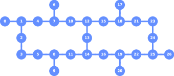
Figure 3: Topology of ibmq_ehningen. The two qubit gate $\operatorname{CX}$ can only be executed between connected qubits.

3.1 IBM quantum backends

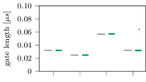
(a) Gate length of $\operatorname{X}$ gate.

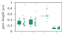
(b) Gate length of two qubit gate.

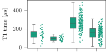
(c) T1 time for each qubit.

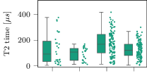
(d) T2 time for each qubit.

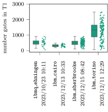
(e) Number of two qubit gates in T1 time.

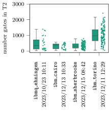
(f) Number of two qubit gates in T2 time.

Figure 47: Gate lengths, coherence times, and number of two qubit gates, that can be executed in the coherence times, of the different backends used in this paper. For the number of gates in the coherence time we used the median of the gate times. The calibration data stems from the dates when the experiments in Section 4.2 and 4.3 were executed. The respective two qubit gate of the backends can be found in Table 1.

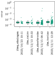
(a) Error of the $\operatorname{X}$ gate.

(b) Error of the two qubit gate.

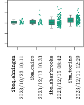
(c) Readout error.

Figure 48: Errors of the hardware gates and of the readout for the different backends used in this paper. We only give the error of the $\operatorname{X}$ and the two qubit gate since the $\operatorname{RZ}$ gate is a virtual gate and thus does not have an error and the error of the $\operatorname{SX}$ gate agrees with the one of the $\operatorname{X}$ gate. The calibration data stems from the dates when the experiments in Section 4.2 and 4.3 were executed. The respective two qubit gate of the backends can be found in Table 1.

As gate-based, universal quantum computers we utilized the superconducting quantum backends of IBM. We mainly employed the ibmq_ehningen backend and for comparison ran our experiments also on the backends ibm_torino, ibm_sherbrooke, and ibm_cairo. Details on the quantum processors of these backends are provided in Table 1. Two important characteristics of the IBM quantum backends is first that they have a limited set of gates that can be executed on the hardware. We will call this set the hardware gates. For all backends that we consider in this article this set consists of the single qubit gates $\operatorname{RZ}$, $\operatorname{SX}=\sqrt{\operatorname{X}}$, and $\operatorname{X}$. Depending on the backend, the two qubit gate is either the $\operatorname{CX}$, $\operatorname{CZ}$, or $\operatorname{ECR}$ gate, see Table 1. Here, $\operatorname{CX}$ is the controlled-$\operatorname{X}$ gate, which we already introduced in (19), $\operatorname{CZ}$ is the analogously defined controlled-$\operatorname{Z}$ gate, and $\operatorname{ECR}$ is the echoed cross-resonance gate [40]. The second key characteristic is that the quantum processors have a topology with limited connectivity in the sense that the hardware two qubit gate can only be executed on certain qubit pairs. We give the topology of ibmq_ehningen in Figure 3 and refer to [39] for the other backends. More details about the backends such as gate errors or coherence times can be found in Figures 47 and 48 in the appendix.

3.2 D-Wave backends

For our quantum annealing experiments we used the D-Wave Advantage 4.1. The specifications of this system are given in Table 2. The Pegasus features qubits of degree 15, i.e. each qubit is coupled to 15 different qubits, and native $K_{4}$ and $K_{6,6}$ subgraphs, see Figure 4. The Pegasus qubits have three different types of couplers which are internal, external and odd: The Pegasus has nominal length of 12 meaning each qubit is connected to 12 orthogonal qubits through internal couplers indicated with green lines in Figure 4 (c). Orthogonal qubits are those that are not connected to each other. The external couplers connect the qubits with the adjacent Pegasus single cells shown with light blue lines in Figure 4 (c). The Pegasus single cell is shown in Figure 4 (a). An odd coupler can only couple to one qubit, which is in the same single Pegasus cell. For example, qubit 4 and 5 are coupled via an odd coupler in Figure 4 (a), also colored pink in Figure 4 (c).

name	topology	# qubits	$\begin{array}[]{c}\text{annealing}\\ \text{range [$\mu$s] }\end{array}$	$\begin{array}[]{c}\text{connectivity}\\ \text{degree}\end{array}$	$\begin{array}[]{c}\text{nominal}\\ \text{length}\end{array}$
Advantage 4.1	Pegasus	5627	0.5 – 2000	15	12

Table 2: Specifications of the D-Wave quantum annealer that was used for the experiments in this article.

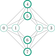
(a) Pegasus single cell.

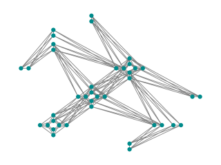
(b) Repetition pattern of Pegasus single cell which forms one unit cell.

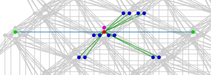
(c) Single qubit connectivity (degree = 15).

Figure 4: Architecture of the D-Wave Advantage 4.1.

Now, let us introduce the embedding which is is a fundamental aspect of utilizing D-Wave quantum annealers. As we have seen, the Advantage 4.1 has a limited connectivity between qubits so that not all problem Hamiltonians can be directly represented on the quantum processing unit (QPU). Minor embedding [41] is the process of mapping a problem’s logical qubits onto the annealer’s physical qubits, forming chains, where necessary. This technique ensures that the logical problem graph is represented within the constraints of the QPU’s architecture, such as Pegasus topologies [42]. Usually, there are many possible embeddings that differ in their quality. Poor embeddings can lead to longer chains of physical qubits, which are more susceptible to errors such as broken chains. These errors occur when the physical qubits in a chain do not all agree on a value, potentially deteriorating the solution quality [43]. Conversely, a good embedding ensures that the problem’s structure is well-represented on the QPU, allowing the quantum annealer to effectively explore the problem’s solution space [44]. However, finding an optimal embedding is challenging and known to be NP-hard, adding complexity to the problem-solving process on D-Wave quantum annealers.

Intimately connected to the embedding is the chain strength. A chain in this context refers to a set of qubits that collectively represent a single variable (i.e. a logical qubit) from the problem being solved. As we have discussed above, chains are required due to the limited connectivity in the QPU. The primary purpose of setting the chain strength is to ensure that all qubits within a chain yield the same value when a computation is performed. This is achieved by applying a strong ferromagnetic coupling between the qubits in a chain, making it energetically favorable for them to align in the same state [45]. The chain strength must be carefully balanced. If it is too small the qubits within a chain may not align, leading to broken chains, where the value of the logical qubit is ambiguous. Conversely, if the chain strength is too high, it can dominate over the problem’s intrinsic couplings which can potentially skew the solution landscape and lead to suboptimal solutions [46].

Last, the annealing time schedule defines the temporal profile of the quantum annealing process, where the system transitions from an initial quantum state to a final state that ideally represents the solution of the optimization problem [47]. The schedule is typically a function that describes how the system’s Hamiltonian changes over time, affecting the dynamics of the annealing process and the likelihood of the system settling into the global minimum energy state. A well-chosen annealing schedule can enhance the probability of finding the optimal solution by carefully managing the rate at which quantum fluctuations are reduced during the annealing process [48]. If the annealing is too rapid, the system may not maintain its ground state, leading to suboptimal solutions. Conversely, if the annealing is too slow, it may become computationally inefficient [49]. Experimentation with different annealing schedules, such as introducing pauses or changes in the annealing rate, can improve performance for certain types of problems [50]. The optimal annealing schedule may vary depending on the specific problem instance, and finding the right balance is often a matter of empirical investigation [48].

4 Use Case 1: Optimization of Charging Schedules

In our first use case we study the optimization of charging schedules for electric vehicles. More precisely, this use case stems from the project LamA (Laden am Arbeitsplatz, in English: charging at the workplace) where a charging infrastructure is built up at 37 institutes of the Fraunhofer society, on which employees can charge their electric vehicles [51]. In this paper we consider a proof of concept (PoC) model that is suitable for the current NISQ era quantum computers. We will only give a short overview here and refer the reader to [21] where the details are elaborated. Owing to the background of this use case we will refer to it as the “LamA use case” throughout this paper.

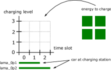
(a) Example series lama_0p* with one car and three time slots.

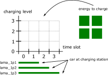
(b) Example series lama_1p* with one car and four time slots.

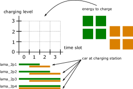
(c) Example series lama_2p* with two cars and four time slots.

Figure 5: Visualization of the three example series for the LamA use case. All series are based on one charging station with four charging levels but differ in the number of cars that are at the charging station and the number of time slots when the car(s) can charge at this station. Within an example series we consider different examples that vary in the time slots when the car(s) are at the charging station.

We consider the PoC model with the following setting: We have a single charging station with four charging levels 0, 1, 2, and 3, and $T$ time slots 0, 1, …, $T-1$ when cars can charge. Moreover, we assume that $K$ cars are charging energy and that the required amount of energy as well as the time slots when each car is at the charging station are known. The aim of our optimization is to calculate a charging schedule that minimizes the peak load. As presented in [21] this can be modeled by a quadratic constrained integer optimization problem of the form (2). Here, the minimization part (2a) is responsible to minimize the peak load wheres the constraint part (2b) ensures that each car charges the right amount of energy in valid time slots. Since we have four charging levels the integer vector $\mathbf{n}$ in (2) is taken from the set $\{0,1,2,3\}^{N}$ where $N=KT$. As we have discussed in Section 2.1 such an optimization problem can be transformed to a QUBO (6b). Since we can encode the four charing levels into two qubits we have $M=2KT$ binary variables $\mathbf{b}\in\{0,1\}^{M}$.

$\begin{array}[]{c}\text{example}\\ \text{series}\end{array}$	$\begin{array}[]{c}\text{\# time slots}\\ T\end{array}$	$\begin{array}[]{c}\text{\# cars}\\ K\end{array}$	$\begin{array}[]{c}\text{\# qubits}\\ M\end{array}$
lama_0p*	3	1	6
lama_1p*	4	1	8
lama_2p*	4	2	16

(a) Number of time slots $T$ when cars can charge at the charging station, number of cars $K$ that are at the station, and number of qubits $M$ that are needed to model the example series.

example	$\begin{array}[]{c}\text{\# optimal }\\ \text{solutions}\end{array}$
lama_0p1	1
lama_0p2	3
lama_1p1	1
lama_1p2	3
lama_1p3	1
lama_2p1	3
lama_2p2	3
lama_2p3	6
lama_2p4	19

(b) Number of optimal solutions.

Table 3: Description of the example series for the LamA use case (a) and number of optimal charging schedules for each example (b).

In this setting we construct three example series lama_0p*, lama_1p*, and lama_2p* of increasing problem sizes (i.e. number of qubits). Within each series we consider different examples of increasing coupling strength which we obtain from iteratively increasing the overlap of time slots when cars charge in parallel. In Figure 5 we visualize the different examples and in Table 3 we give the problem parameters and required number of qubits. The different coupling strengths of the examples in every example series is directly reflected in the sparsity pattern of the associated QUBO matrix $\mathbf{Q}$, see Figure 6. We already note here that the sparsity pattern will have a strong impact on the depth of the QAOA circuits and through this on the quality of results from real quantum backends.

(a) lama_0p1.

(b) lama_0p2.

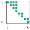
(c) lama_1p1.

(d) lama_1p2.

(e) lama_1p3.

(f) lama_2p1.

(g) lama_2p2.

(h) lama_2p3.

(i) lama_2p4.

Figure 6: Spy plot of the QUBO matrix $\mathbf{Q}=(q_{ij})_{i,j=1}^{M}$ for the examples in the LamA use case. A marker indicates a non-zero matrix entry $q_{ij}\neq 0$, whereas a missing marker means $q_{ij}=0$.

4.1 Classical optimization

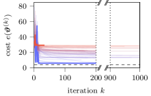
(a) QAOA, $L=1$, $P=2$.

(b) QAOA, $L=2$, $P=4$.

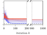
(c) QAOA, $L=3$, $P=6$.

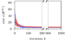
(d) VQE, $L=1$, $P=16$.

(e) VQE, $L=2$, $P=24$.

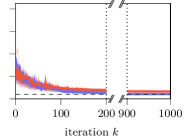
(f) VQE, $L=3$, $P=32$.

Figure 7: Convergence of the classical optimizer COBYLA used to minimize the cost $e(\bm{\vartheta})$ for QAOA (upper plots) and VQE (lower plots) applied to lama_1p3. For both algorithms different number of layers $L$ have been used (left to right), which result in different numbers $P$ of parameters that are optimized. Each line stems from one of 50 optimization runs, where each run was provided with a different, random initial guess $\bm{\vartheta}^{(0)}$. The color of the lines indicate the final cost $e(\bm{\vartheta}^{\mathrm{final}})$. The best and the worst run are indicated with a bold line. The optimization was stopped when the default termination criterion of COBYLA was satisfied or after the default maximum number of 1000 iterations. The quantum circuits were executed with an exact simulation. The dashed line indicates the cost of the exact solution $\mathbf{b}^{\star}$.

As described in Section 2.2, we can derive a problem Hamiltonian $H_{P}$ from the QUBO formulation of our LamA use case examples. Then, we have all ingredients to built the QAOA and VQE circuits given in (13e) and (18), respectively. In this section we are concerned with the finding of optimal variational parameters, i.e. $(\bm{\beta}^{\diamond},\bm{\gamma}^{\diamond})$ for QAOA and $\bm{\theta}^{\diamond}$ for VQE. Recall that these parameters are the solutions of the minimization problems (13f) and (17), respectively. In the subsequence we just write $\bm{\vartheta}$ and

$$\bm{\vartheta}^{\diamond}=\operatorname*{arg\,min}_{\bm{\vartheta}}e(\bm{\vartheta})\,,\qquad e(\bm{\vartheta})=\left\langle H_{P}\right\rangle_{\left|\psi(\bm{\vartheta})\right\rangle}\,,$$ (20)

as a generic minimization problem fitting both for QAOA and VQE. For this minimization problem $e$ plays the role of the cost function. Its connection to the QUBO cost function $f$ is given by (10).

Among the wide variety of classical optimizers that can be used to (approximately) solve the minimization task (20) we selected the local optimizer COBYLA (as it is implemented in qiskit with its default parameters) for the LamA use case. This optimizer computes iteratively a sequence of parameters $\{\bm{\vartheta}^{(j)}\}$ that should approximate the minimum of $e$, i.e. $e(\bm{\vartheta}^{(j)})\approx e(\bm{\vartheta}^{\diamond})$ for $j$ large enough. To start this sequence, the user has to provide an initial guess $\bm{\vartheta}^{(0)}$. As we will see below, this choice can have a strong influence on the sequence of parameters $\{\bm{\vartheta}^{(j)}\}$. In order to compute a new iterate $\bm{\vartheta}^{(j+1)}$ the cost function $e$ has to be evaluated. It is important to note that evaluating the cost function for a certain choice of parameters $\widetilde{\bm{\vartheta}}$ requires that the QAOA or VQE circuit have to be executed either on a simulator or on a real quantum backend. However, only on an exact simulator $|\psi(\widetilde{\bm{\vartheta}})\rangle$ and thus $\left\langle H_{P}\right\rangle_{|\psi(\widetilde{\bm{\vartheta}})\rangle}$ can be obtained. For a noisy simulator or a real quantum backend only approximations to this expectation can be obtained as we will discuss further below.

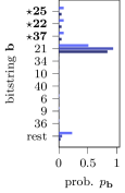
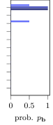
(a) lama_0p2.

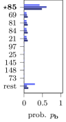
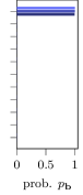
(b) lama_1p3.

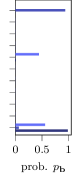
(c) lama_2p3.

Figure 8: Probabilities $p_{\mathbf{b}}(\bm{\vartheta}^{\diamond})$ for the best variational parameters $\bm{\vartheta}^{\diamond}$ found with the optimizer COBYLA. In each subplot the left figure stems from the QAOA circuit and the right from the VQE circuit, where the number of layers $L$ is indicated by the color of the bar. The bitstrings $\mathbf{b}$ are sorted by cost (lower cost on top), denoted in integer notation, and only the ten with the lowest cost are displayed. The optimal QUBO solution(s) are marked in bold and with a $\star$. Note that the convergence plots for the variational parameters can be found in Figure 7 for lama_1p3 and in Figure 46 for lama_0p2 and lama_2p3.

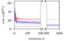
(a) QAOA, $L=1$, $P=2$.

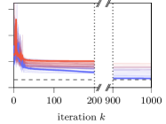
(b) QAOA, $L=2$, $P=4$.

(c) QAOA, $L=3$, $P=6$.

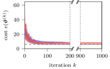
(d) VQE, $L=1$, $P=12$.

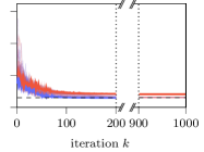
(e) VQE, $L=2$, $P=18$.

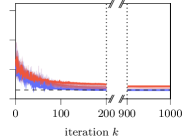
(f) VQE, $L=3$, $P=24$.

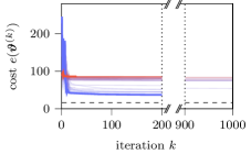
(g) QAOA, $L=1$, $P=2$.

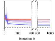
(h) QAOA, $L=2$, $P=4$.

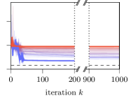
(i) QAOA, $L=3$, $P=6$.

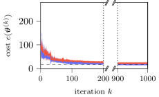
(j) VQE, $L=1$, $P=32$.

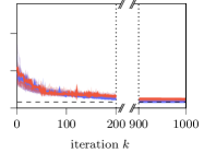
(k) VQE, $L=2$, $P=48$.

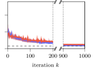
(l) VQE, $L=3$, $P=64$.

Figure 46: Convergence of the classical optimizer COBYLA for lama_0p2 (two upper rows) and lama_2p3 (two lower rows). The setup is the same as described in Figure 7.

The first experiment we want to report here is concerned with optimizing the QAOA and VQE parameters for the fully coupled, eight qubit example lama_1p3 for circuits with $L=1$, $2$, and $3$ layers. We used an exact simulation to execute the circuits and ran the COBYLA optimization 50 times, where in each run we used a different, randomly generated initial guess $\bm{\vartheta}^{(0)}$. In Figure 7 we show the cost $e(\bm{\vartheta}^{(k)})$ versus the iteration number $k$, where every line stems from one of the 50 initial guesses. Thereby, the color scale indicates the final cost $e(\bm{\vartheta}^{\mathrm{final}})$, which is either when the (default) termination criterion is satisfied or after the default maximum number of 1000 iterations. We use a color scale from blue (lowest cost) to red (highest cost). Additionally, we marked the two iterations that lead to the lowest and to the highest final cost with a bold line. For QAOA we can see a strong dependency of the final cost on the initial guess. Moreover, we see that for QAOA the optimizer converged fast and the optimization only continued because the default stopping criterion does not work well. For VQE the convergence is on the one hand slower but on the other hand the dependency on the initial guess is much less pronounced compared to QAOA. The reason for both observations could be that in QAOA only $P=2L$ parameters have to be optimized, whereas in VQE we have $P=M(L+1)=8(L+1)$ parameters. For VQE this gives the optimizer the freedom to drive any given initial guess to a good solution, however at the cost of having to search in a much larger space of parameters. The convergence plots for lama_0p2 and lama_2p3 are given in Figure 46 in the Appendix.

Recall from (11b) that the aim of optimizing the variational parameters is to obtain a circuit that generates a state $\left|\psi(\bm{\vartheta}^{\diamond})\right\rangle=\sum_{\mathbf{b}\in\{0,1\}^{M}}a_{\mathbf{b}}(\bm{\vartheta}^{\diamond})\left|\mathbf{b}\right\rangle$ which has an amplitude $a_{\mathbf{b}^{\star}}(\bm{\vartheta}^{\diamond})$ with large absolute value for the basis state $\left|\mathbf{b}^{\star}\right\rangle$ of the exact solution of our QUBO. In order examine if our optimization was able to achieve this we order the bitstrings $\mathbf{b}_{1},\mathbf{b}_{2},\dots,\mathbf{b}_{2^{M}}$ in $\{0,1\}^{M}$ with respect to their cost, i.e. $e(\mathbf{b}_{1})\leq e(\mathbf{b}_{2})\leq\dots\leq e(\mathbf{b}_{2^{M}})$. For a shorter notation we write the bitstrings in integer notation, i.e. for $\mathbf{b}=(b_{1},\dots,b_{M})$ we write $n=\sum_{i=1}^{M}b_{i}2^{i-1}$. As optimal parameters $\bm{\vartheta}^{\diamond}$ we take $\bm{\vartheta}^{\mathrm{final}}$ from the optimization pass that yielded the lowest cost, i.e. we take the best parameters that were found in the 50 optimizations. In Figure 8 we show $p_{\mathbf{b}_{i}}(\bm{\vartheta}^{\diamond})=|a_{\mathbf{b}_{i}}(\bm{\vartheta}^{\diamond})|^{2}$ for the ten best bitstrings $\mathbf{b}_{i}$, $i=1,\dots,10$, for lama_0p2, lama_1p3, and lama_2p3, and for both QAOA and VQE with $L=1$, $2$, and $3$ layers. We see that for the two smaller examples VQE is able to generate states which solely contain optimal solution bitstrings (marked in bold and with a $\star$ in the plots). Even for the largest example and $L=2$ this is almost the case. On the other hand, QAOA generates for lama_0p2 and all layer numbers states that have their largest amplitude for a bitstring that has the second smallest cost. For lama_1p3 the largest amplitude is for the correct bitstring but with a smaller absolute value square than for VQE. Finally, for lama_2p3 QAOA is not able to generate a state with amplitudes that have an absolute value notably above zero for the ten bitstrings with the lowest cost.

Last in this section, let us recall that on real quantum backends we do not have access to the amplitudes of a quantum state but only to an approximation $\widetilde{p}_{\mathbf{b}}$ of the probabilities $p_{\mathbf{b}}=|a_{\mathbf{b}}|^{2}$. The probability distribution $\{\widetilde{p}_{\mathbf{b}}\}$ is obtained from executing and measuring the quantum circuit for $S$ times, where each cycle is called a shot. Thus, the error between $\widetilde{p}_{\mathbf{b}}$ and $p_{\mathbf{b}}$ is called shot noise. This is not connected to hardware errors but would be present even for an error free quantum computer. Such an error free quantum computer can be emulated with an exact simulator with shot noise. For such an simulator we show in Figure 9 the results for $S=1000$ shots of the exact same experiments as above with the exact, shot noise free simulator. We see that for QAOA the optimizer terminates much earlier but with a higher cost function value. The strong dependency on the initial guess is still present and even more pronounced towards optimization passes that end with a high cost function value. For VQE we observe that the initial value now has a slightly stronger influence and that the final cost is also slightly higher compared to the shot noise free simulation.

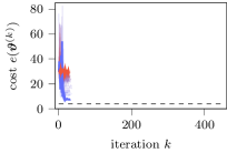
(a) QAOA, $L=1$, $P=2$.

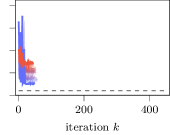
(b) QAOA, $L=2$, $P=4$.

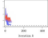
(c) QAOA, $L=3$, $P=6$.

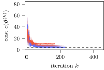
(d) VQE, $L=1$, $P=12$.

(e) VQE, $L=2$, $P=18$.

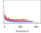
(f) VQE, $L=3$, $P=24$.

Figure 9: Convergence of the classical optimizer COBYLA for lama_1p3 in the same situation as in Figure 7 except that an exact simulation with shot noise is used to execute the quantum circuits. The number of shots is set to $S=1000$.

We close this section with remarking that we ran all the upper classical optimizations for 10 different values of the penalty parameter $\varrho$. More precisely, we calculated the minimum penalty $\varrho_{\mathrm{min}}$ that ensures that the solution of the QUBO (6b) is also the solution of the original problem (2) and considered the values $\varrho=\varrho_{\mathrm{min}}+0.1k$, $k=0,\dots,9$. The results from above stem from the penalty that gave the lowest cost in the classical optimization. This penalty is also used for all results on quantum computing backends that follow in the subsequence.

4.2 Experiments on ibmq_ehningen

In this section we present experiments on the 27 qubit backend ibmq_ehningen. Experiments on the backends ibm_torino, ibm_sherbrooke, and ibm_cairocan be found in Section 4.3.

Transpilation

As a first step the logical QAOA and VQE circuits, recall Figures 1 and 2, respectively, have to be transpiled to circuits that can be executed on ibmq_ehningen. Recalling Section 3.1 on the IBM quantum systems, among others, the transpilation has to route multi-qubit gates such that they match the topology of ibmq_ehningen, see Figure 3, and it has to synthesize the logical gates into the hardware gates $\operatorname{RZ}$, $\operatorname{X}$, $\operatorname{SX}$, and $\operatorname{CX}$. Of all hardware gates the $\operatorname{CX}$ gate has by far the largest error, see Figure 48, and thus will contribute the dominant gate error part of a quantum circuit. Consequently, we are mostly interested in the $\operatorname{CX}$ gates in the transpiled quantum circuit and will neglect the transpilation of single qubit gates.

[row sep=0.6cm, between origins] $\scriptstyle q_{0}$ & 2 [3,brackets=none]= 1
$\scriptstyle q_{1}$ 1
$\scriptstyle q_{2}$ aaaaa RZZ(θ) aaaaa RZZ(θ)

(a) Performing a $\operatorname{RZZ}$ gate on two qubits without physical connection (compare qubits 0 and 2 in Figure 3) requires $\operatorname{SWAP}$ gates.

& 1 [2,brackets=none]= 1 1
-1

(b) A $\operatorname{SWAP}$ gate can be decomposed into three $\operatorname{CX}$ gates.

Figure 10: A $\operatorname{RZZ}$ gate for unconnected qubits requires the insertion of $\operatorname{SWAP}$ gates which can be decomposed into $\operatorname{CX}$ gates.

Now, let us look deeper into the transpilation of our QAOA and VQE circuits: Recall that for the QAOA algorithm (13f) we derived the gate representation of the involved operators in (14), (15), and (16). There, we see that the only multi-qubit gate in the logical quantum circuit is the $\operatorname{RZZ}$ gate. For the VQE algorithm with the two-local ansatz (18) the only multi-qubit gate is the $\operatorname{CX}$ gate. To match the topology of ibmq_ehningen the transpilation has to add $\operatorname{SWAP}$ gates for all two qubit gates that act on two qubits that are not connected. For example an $\operatorname{RZZ}$ gate on qubits 0 and 2 requires a $\operatorname{SWAP}$ gate between qubits 0 and 1, compare Figure 10(a). Each $\operatorname{SWAP}$ gate in turn can be decomposed into three $\operatorname{CX}$ gates, see Figure 10(b). Moreover, an $\operatorname{RZZ}$ gate can be decomposed into two $\operatorname{CX}$ gates and one $\operatorname{RZ}$ gate, see Figure 11.

& 1 [2,brackets=none]= 1 1
aaaaa RZZ(θ) RZ(θ)

Figure 11: Decomposition of the $\operatorname{RZZ}$ gate into one $\operatorname{RZ}$ and two $\operatorname{CX}$ gates.

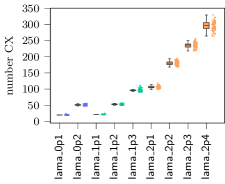
(a) QAOA.

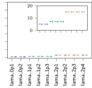
(b) VQE.

Figure 12: Number of $\operatorname{CX}$ gates in the transpilations of the QAOA (left) and VQE (right) circuits to the backend ibmq_ehningen for the LamA use case examples. The transpilation was carried out with the qiskit transpiler on optimization_level 3. Every circuit was transpiled 75 times, where for each transpilation a different transpilation seed was used. For every example each dot in the figures represents the number of $\operatorname{CX}$ gates from one such transpilation.

With these considerations in mind, let us now look at the transpilations of the logical QAOA and VQE circuits for all our LamA examples which we obtained by using the qiskit transpiler. Clearly, there are many possibilities how our logical circuits can be transpiled to ibmq_ehningen and finding the best transpilation is a non-trivial task. In order to control how much optimization is performed on this task the qiskit transpiler offers four optimization_levels 0, 1, 2, and 3. Moreover, it is important to know that the transpiler has stochastic components which can be controlled with a so-called random seed. In Figure 12 we show the number of $\operatorname{CX}$ gates for the transpilations of the QAOA and VQE circuits to ibmq_ehningen for 75 different seeds and for the highest optimization_level 3. Let us first look at the VQE circuits in Figure 12(b). There, we see that the number of $\operatorname{CX}$ gates is the same for every example of an example series. This is due to the fact that only the number of qubits enters in our VQE algorithm (18) and this number is the same for all examples of an example series, see Table 3(a). Moreover, we only observe a slight increase in the number of $\operatorname{CX}$ gates from lama_0p* to lama_1p* to lama_2p*. Besides the increasing qubit number the reason lies in the insertion of $\operatorname{SWAP}$ gates which are necessary to perform $\operatorname{CX}$ gates between unconnected qubits. However, due to the linear entanglement structure in our VQE ansatz only few $\operatorname{SWAP}$ gates are needed. The simplicity of this ansatz is also reflected in the fact that every transpilation seed results in a circuit with the same number of $\operatorname{CX}$ gates. For the QAOA circuits we observe a completely different behavior, see Figure 12(a). First of all, the (median) number of $\operatorname{CX}$ gates is not constant within the example series but different for each individual example. In order to understand this, first note that the problem Hamiltonian $H_{P}$ enters in the phase operator $U_{P}$, see (13b), and thus the QAOA circuit depends on it. In particular, by recalling (15) we see that the off-diagonal non-zero entries $h_{ij}\neq 0$, $i\neq j$, of the problem Hamiltonian $H_{P}$ induce the $\operatorname{RZZ}_{i,j}$ gates in the QAOA circuits. It is easy to show that $h_{ij}\neq 0$ if and only if $q_{ij}\neq 0$, where $q_{ij}$ is the $(i,j)$th entry of the QUBO matrix $\mathbf{Q}$, see (8). This means that the sparsity pattern (the non-zero entries) of the QUBO matrix is directly connected to the number of $\operatorname{RZZ}$ gates in the logical QAOA circuits. Recall from above that it is precisely the $\operatorname{RZZ}$ gates that generate the $\operatorname{CX}$ gates in the transpilation. Thus, one reason for the different number of $\operatorname{CX}$ gates for every example is that the sparsity pattern of the QUBO matrices of our examples, see Figure 6, are all different. Moreover, the insertion of $\operatorname{SWAP}$ gates that are needed to realize $\operatorname{RZZ}$ gates between unconnected qubits increases the number of $\operatorname{CX}$ gates in the transpiled circuits. Note that due to the low connectivity of ibmq_ehningen, recall Figure 3, the denser the QUBO matrices are (the more non-zero entries they have) the stronger this effect is. We can see this e.g. by comparing lama_0p2 and lama_1p2 or lama_1p3 and lama_2p1, where the example with less qubits but denser QUBO matrix has a similar number of $\operatorname{CX}$ gates than the example with the higher qubit number but sparser QUBO matrix. Last, let us remark that the deviation of the $\operatorname{CX}$ numbers for a fixed example is due to the optimization potential and the stochastic part in the transpilation. This optimization potential is the higher the deeper the circuits get as can be seen by comparing the variances from the smaller example series with the larger ones.

Cost landscape

Recall from (13f) and (20) that we are interested in finding the QAOA parameters $\bm{\beta}$ and $\bm{\gamma}$ that minimize $e(\bm{\beta},\bm{\gamma})=\left\langle H_{P}\right\rangle_{\left|\psi_{\mathrm{QAOA}}(\bm{\beta},\bm{\gamma})\right\rangle}$. For QAOA with $L=1$ layer we only have two parameters $\bm{\beta}=\beta$ and $\bm{\gamma}=\gamma$, and thus can visualize the cost

$$e(\beta,\gamma)=\left\langle H_{P}\right\rangle_{|\psi_{\mathrm{QAOA}}(\beta,\gamma)\rangle}\,,\qquad\beta,\gamma\in[0,\pi]\,,$$

as a heat map. For this we discretized the interval $[0,\pi]$ into $50$ grid points for both $\beta$ and $\gamma$, and then computed $e(\beta,\gamma)$ for each of the $50\cdot 50=2500$ grid points. Note that each evaluation of $e(\beta,\gamma)$ requires the execution of one QAOA circuit. In Figure 13 we show the resulting cost landscape for lama_1p3, where the QAOA circuits were executed either with an exact simulation with shot noise (Figure 13(a)), a simulation with a noise model of ibmq_ehningen (Figure 13(b)), or on the ibmq_ehningen backend. In all three cases the number of shots was set to $S=1000$. For ibmq_ehningen a transpilation with optimization_level 3 and measurement error mitigation was used. Comparing the result from ibmq_ehningen with the exact simulation we clearly see that most of the signal is lost and only few details of the cost landscape can be resolved. The simulation with the noise model predicts a loss of signal and details but by far not as strong as obtained from the real backend. Moreover, we see that the cost landscapes have different scales. In fact, the minimum and maximum for the exact simulation are $8.04$ and $95.56$, for the simulation with the noise model $14.51$ and $63.53$, and for ibmq_ehningen $0.0$ and $52.52$. In Figures 13(d) and 13(e) we give the cost landscapes for the simulation with the noise model and ibmq_ehningen on a zoomed color scale. Also on this scale the signal of ibmq_ehningen is weak and much noisier than the simulation with the noise model predicts. This already hints that optimizing the variational parameters $\bm{\beta}$ and $\bm{\gamma}$ on the real quantum computer is a difficult task. We will take a closer look at this in the next paragraph.

(a) Exact simulation with shot noise.

(b) Simulation with noise model of ibmq_ehningen.

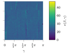
(c) ibmq_ehningen.

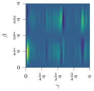
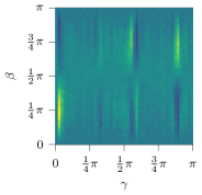
(d) Simulation with noise model
of ibmq_ehningen.

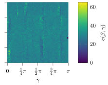
(e) ibmq_ehningen.

Figure 13: Heat map of the cost $e(\beta,\gamma)$, for $\beta,\gamma\in[0,\pi]$, QAOA with $L=1$ layer, and lama_1p3. The interval $[0,\pi]$ was discretized in 50 grid points for both $\beta$ and $\gamma$. The QAOA circuit was executed with three different backends: exact simulator with shot noise (a), simulator with noise model of ibmq_ehningen (b) and (d), and ibmq_ehningen (c) and (e). For all backends the number of shots was set to $S=1000$. The results for ibmq_ehningen stem from three sessions that ran on 2023/11/08, 2023/11/09, and 2023/11/10. The noise model is from 2023/11/10. For the (a) – (c) the color scale ranges from $0$ to $95$ and for (d) and (e) from $0$ to $65$.

Classical optimization on ibmq_ehningen

In Section 4.1 we studied the optimization of the parameters $\bm{\beta}$ and $\bm{\gamma}$ for QAOA and $\bm{\theta}$ for VQE with the COBYLA optimizer in combination with an exact simulator with and without shot noise to execute the quantum circuits. Now, we use the same optimizer with the same settings (except we limit the maximum number of function evaluations to 50) but execute the circuits on the ibmq_ehningen backend. We do this only for the two best and two worst initial guesses, that we found when using the exact simulator. In Figure 14 we show the results for lama_0p2, lama_1p3, and lama_2p4 for QAOA and VQE. In low opacity we added the result of the exact simulator. We can clearly see that for the smallest example the QAOA parameters can be determined with ibmq_ehningen with a cost function value comparable to the one of the exact simulator. However, for the two larger examples we see (nearly) no convergence and no agreement with the exact simulation. A meaningful optimization does not take place. In contrary, we see a good agreement for VQE for the smaller examples, and even for the largest example we can recognize a convergence behavior.

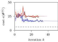
(a) lama_0p2, QAOA.

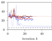
(b) lama_1p3, QAOA.

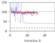
(c) lama_2p4, QAOA.

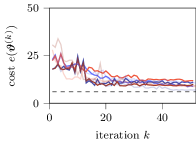
(d) lama_0p2, VQE.

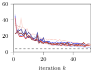
(e) lama_1p3, VQE.

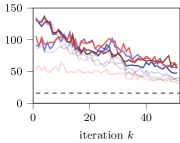
(f) lama_2p4, VQE.

Figure 14: Convergence of the classical optimizer COBYLA used to minimize the cost $e(\bm{\vartheta})$ for QAOA (upper plots) and VQE (lower plots) applied to lama_0p2, lama_1p3, and lama_2p4 (left to right). For both algorithms $L=1$ layer was used. As initial guess $\bm{\vartheta}^{(0)}$ the two best (blue lines) and the two worst (red lines) choices, that have been identified with an exact simulation (compare Figure 7), were used. The quantum circuits were executed on ibmq_ehningen using qiskit’s Estimator primitive with resilience_level 1 and optimization_level 3. In order to save quantum computing resources the maximum number of iterations was limited to 50 and the number of shots was chosen as 1000. The optimization was stopped when the default termination criterion of COBYLA was satisfied or after the maximum number iterations was reached. The dashed line indicates the cost of the exact solution $\mathbf{b}^{\star}$ and the transparent lines show the convergence of the exact simulation. The circuits for the plots (a) – (f) were executed on 2023/10/24 11:13, 2023/10/23 22:48, 2023/10/26 20:26, 2023/10/25 11:24, 2023/10/24 12:39, and 2023/10/27 21:37, respectively.

4.2.1 Quality of results

In the next paragraphs we are concerned with the question of how well our QAOA and VQE circuits can be executed on today’s error-prone quantum hardware. For this purpose we will only execute fully trained circuits, where we take the best values for our variational parameters that we have found in the above optimization runs. Before we present the results let us introduce some notations: Let us consider a fully trained circuit and let us denote with

$$|\widehat{\psi}\rangle=\sum_{\mathbf{b}\in\{0,1\}^{M}}\widehat{a}_{\mathbf{b}}\left|\mathbf{b}\right\rangle$$

the state that such a circuit generates. Using an exact simulation we can access $|\widehat{\psi}\rangle$ and, in particular, we can calculate the probability distribution $\{\widehat{p}_{\mathbf{b}}\}$ by $\widehat{p}_{\mathbf{b}}=|\widehat{a}_{\mathbf{b}}|^{2}$. Now, let us denote with $|\widetilde{\psi}\rangle$ the state that a real quantum computer generates when it executes the same circuit. Then, we do not have access to the quantum state $|\widetilde{\psi}\rangle$ but only to the probability distribution $\{\widetilde{p}_{\mathbf{b}}\}$ that we obtain from $S$ shots of executions and measurements of the circuit. In this paper we will consider two metrics to measure the quality of $\{\widetilde{p}_{\mathbf{b}}\}$.

The first metric is the Hellinger fidelity defined by

$$F=F\bigl{(}\{\widehat{p}_{\mathbf{b}}\},\{\widetilde{p}_{\mathbf{b}}\}\bigr{)}=\left(\sum_{\mathbf{b}\in\{0,1\}^{M}}\sqrt{\widehat{p}_{\mathbf{b}}\;\widetilde{p}_{\mathbf{b}}}\right)^{2}\,.$$ (21)

For this metric we have $F\in[0,1]$, where $F\approx 1$ indicates a high agreement of the result from the real computer with the simulation whereas $F\approx 0$ indicates a poor agreement. Note that the fidelity is problem agnostic, so that a high fidelity does not necessarily mean that $|\widetilde{\psi}\rangle$ yields a good solution for our underlying QUBO problem. This is different for the second metric we consider, namely the relative error

$$E\bigl{(}\{p_{\mathbf{b}}\}\bigr{)}=\frac{1}{f^{\star}}\bigl{|}e(\{p_{\mathbf{b}}\})-f^{\star}\bigr{|}\,,\qquad f^{\star}=f(\mathbf{b}^{\star})\,,$$ (22a)

where $$\mathbf{b}^{\star}$$ is the solution of our QUBO (7) and where in analogy to (10) we define

$$e(\{p_{\mathbf{b}}\})=\sum_{\mathbf{b}\in\{0,1\}^{M}}p_{\mathbf{b}}f(\mathbf{b})\,.$$ (22b)

If $E\bigl{(}\{p_{\mathbf{b}}\}\bigr{)}\approx 0$ then we have a good approximation to the solution of our QUBO in the sense of (11b).

In the now following we will report and discuss results from ibmq_ehningen. Results from other quantum backends then follow in Section 4.3.

Setup

As we have discussed further above, before circuits can be executed on a quantum computer they have to be transpiled. We have seen that this step is not deterministic and, depending on the transpilation seed, we can obtain circuits with different numbers of gates. Moreover, all our examples use less than the 27 qubits that ibmq_ehningen provides. Thus, transpilations with different seeds could use different qubits, which in turn can have different error rates. In order to account for this we transpile every logical circuit 75 times, where we use a different transpilation seed each time. We run all of the resulting 75 transpiled circuits and will always report on all their outcomes in the subsequence. We always use measurement error mitigation as provided by resilience_level 1 of qiskit’s Sampler primitive and $S=10000$ shots. Moreover, we use a $\operatorname{X}$–$\operatorname{X}$ dynamical decoupling sequence as a simple but powerful technique to strengthen the resilience of the qubits [52, 53]. In order to show the differences we always report results once without and once with dynamical decoupling.

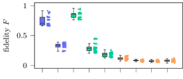
(a) QAOA, w/o dynamical decoupling.

(b) VQE, w/o dynamical decoupling.

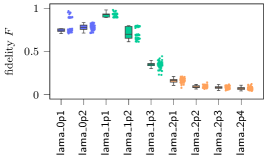
(c) QAOA, w/ dynamical decoupling.

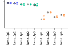
(d) VQE, w/ dynamical decoupling.

Figure 15: Fidelity $F$, as defined in (21), obtained from executing the QAOA (left) and VQE (right) circuits with $L=1$ layer for all LamA use case examples on ibmq_ehningen. We used the best values for the variational parameters that we found with the optimizer COBYLA and an exact simulation, see Section 4.1. For each example, the logical circuit was transpiled 75 times, using a different transpilation seed each time. Each dot stems from such a transpilation. We ran the resulting circuits with (bottom) and without (top) dynamical decoupling. The number of shots was set to $S=10000$. All circuits were ran within a single qiskit session, where the first circuit ran on 2023/10/23 12:03.

Fidelity

In Figure 15 we show the fidelity $F$ obtained from running the QAOA and VQE circuits on ibmq_ehningen for all LamA examples. For QAOA we observe that without dynamical decoupling only lama_0p1 and lama_1p1, i.e. the small and weakly coupled examples, can be carried out with high fidelity. The larger examples, in particular all examples in example series lama_2p* and the stronger coupled examples of series lama_0p* and lama_1p* only achieve a poor fidelity. This can be improved by using dynamical decoupling so that also lama_0p2 and lama_1p2 can be carried out with higher fidelity. However, example series lama_2p* stays infeasible for ibmq_ehningen. On the other hand, the VQE circuits can be carried out on ibmq_ehningen with a rather high fidelity for both example series lama_0p* and lama_1p*. In particular, with dynamical decoupling the fidelity is always close to $1$. However, for all examples from lama_2p* the fidelity drops significantly. Only with dynamical decoupling we obtain a fidelity around 0.5. Recalling from Figure 12 that all VQE circuits have nearly the same amount of $\operatorname{CX}$ gates it is surprising that the lama_2p* series yields such bad fidelities.

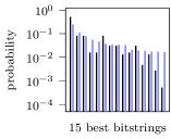
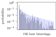
(a) QAOA, lama_0p2.

(b) QAOA, lama_1p3.

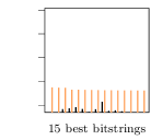
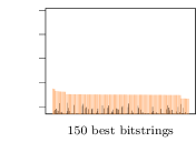
(c) QAOA, lama_2p3.

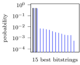
(d) VQE, lama_0p2.

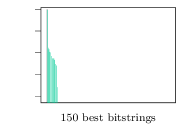
(e) VQE, lama_1p3.

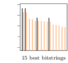
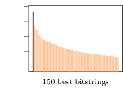
(f) VQE, lama_2p3.

Figure 16: Probabilities $\widetilde{p}_{\mathbf{b}}$ resulting from executing the QAOA (top) and VQE (bottom) circuits with $L=1$ layer for different LamA use case examples on ibmq_ehningen (colored bars). The results stem from the experiment described in Figure 15 and we show the case of the best transpilation seed (with respect to the fidelity) and with dynamical decoupling. In each subfigure we show the 15 (upper plot) and 150 (lower plot) highest probabilities. For clarity we do not show the associated bitstrings but only refer to them as the 15 or 150 best bitstrings. The black bars are the probabilities $\widehat{p}_{\mathbf{b}}$ for those bitstrings but stemming from using an exact simulator instead of ibmq_ehningen.

This becomes clearer when analyzing the probability distributions $\{\widetilde{p}_{\mathbf{b}}\}$ that we obtain from
ibmq_ehningen for the different examples. We show them in Figure 16 for lama_0p2, lama_1p3, and lama_2p3, for the best transpilation seed and with dynamical decoupling. More precisely, we show the 150 of the $2^{M}$ pairs $(\mathbf{b},\widetilde{p}_{\mathbf{b}})$ with the highest probability $\widetilde{p}_{\mathbf{b}}$. On the $x$-axis we have the bitstring $\mathbf{b}$ whose value we do not show to keep a clear figure. On the $y$-axis we plot the respective probability $\widetilde{p}_{\mathbf{b}}$. Note that on this axis we are using a logarithmic scale. As comparison we plot in black the probability $\widehat{p}_{\mathbf{b}}$ of the exact simulation. In good accordance with the QAOA fidelity plot in Figure 15(c) we see that for lama_0p2 we obtain a probability distribution $\{\widetilde{p}_{\mathbf{b}}\}$ from ibmq_ehningen that has large values on similar bitstrings as the exact simulation. However, it is not able to resolve the details correctly. For lama_1p3 we see that the peak probabilities of the exact simulation can only be reached very poorly. Finally, for lama_2p3 we see that the probability distribution of ibmq_ehningen does not match the simulation at all. Let us also emphasize that the probability distributions generated by the QAOA circuits are complicated and that for example a probability of $10^{-3}$ corresponds to only $10$ of our $10000$ shots. In the case of VQE we see that the probability distributions of ibmq_ehningen match very well with those of the simulation for lama_0p2 and lama_1p3. Only a few $\widetilde{p}_{\mathbf{b}}$ are incorrectly non-zero, however their size is at least two magnitudes lower than the $\widetilde{p}_{\mathbf{b}}$ that have correctly non-zero values. This matches perfectly with the fidelity plots in Figure 15(d). For lama_2p3 we see that the two best bitstrings agree with the simulation but their probability is much lower. Furthermore, we see many incorrect probabilities also in the regime of $10^{-1}$ to $10^{-2}$. This explains the bad fidelity we observed in Figure 15(d). It is rather the number of qubits and the associated chances for errors than the number of $\operatorname{CX}$ gates (which are only 15) that cause the bad fidelity. One can make this clear by computing that for lama_0p2 and lama_1p3 we only have $2^{6}=64$ and $2^{8}=256$, respectively, possible bitstrings, whereas for lama_2p3 there are $2^{16}=65536$ possibilities.

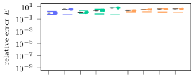
(a) QAOA, w/o dynamical decoupling.

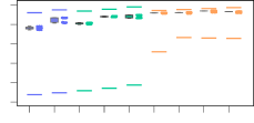
(b) VQE, w/o dynamical decoupling.

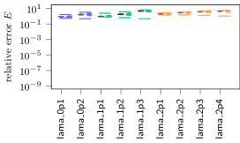
(c) QAOA, w/ dynamical decoupling.

(d) VQE, w/ dynamical decoupling.

Figure 17: Relative error $E$, as defined in (22b), obtained from executing the QAOA (left) and VQE (right) circuits with $L=1$ layer for all LamA use case examples on ibmq_ehningen. The results stem from the same experiment as described in Figure 15. The lower horizontal lines indicate the relative error when using an exact simulator instead of ibmq_ehningen. The upper lines stem from the mean of the relative error of the probability distributions of 50 random statevectors.

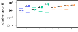
(a) QAOA, w/o dynamical decoupling.

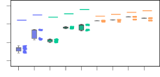
(b) VQE, w/o dynamical decoupling.

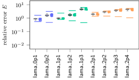
(c) QAOA, w/ dynamical decoupling.

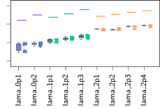
(d) VQE, w/ dynamical decoupling.

Figure 18: Zoom-in for Figure 17.

Figure 19: Legend for scatter plots.

Relative error

Now, let us look at the relative error $E$ that we defined in (22b). In Figure 17 we show $E(\{\widetilde{p}_{\mathbf{b}}\})$ for all LamA examples for QAOA and for VQE, and in Figure 18 we show the same data but with a zoomed-in $y$-axis. For comparison we also added the error for the probability distribution obtained with an exact simulation $E(\{\widehat{p}_{\mathbf{b}}\})$ (the lower lines in the plots). Moreover, we added the error of a random probability distribution. For this we used the probabilities of 50 random statevector and calculated the mean of the relative error of each. In the plots these are the upper lines. In Figure 17 we can see clearly that already the error for the exact simulation of QAOA are magnitudes larger than for VQE. However, this small error for VQE cannot be obtained from ibmq_ehningen. Nevertheless it is much smaller than the error obtained from QAOA on ibmq_ehningen. Looking at the details in Figure 18 we see that except for the small and weakly coupled examples lama_0p1 and lama_1p1 the error of QAOA is rather in the realm of the random guess. VQE stays away from the random guess, but we can see how the error increases with the size of the examples.

Relation between fidelity and relative error

Now, let us look at the relation between the relative error $E$ and the fidelity $F$. In Figure 20 we show this for all LamA examples. For VQE we can clearly see that in the regime $F>0.5$ a higher fidelity $F$ yields a better error $E$. For fidelities below $0.5$ we see that the error stays (approximately) on a plateau. For QAOA the situation is more complicated. In the case of dynamical decoupling we can again see that a higher fidelity gives a smaller error. In the case without dynamical decoupling we observe a plateau for the error in the regime $F>0.5$ and a cluster for $F<0.5$.

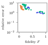
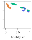
(a) QAOA, w/o (left) and w/ (right) dynamical decoupling.

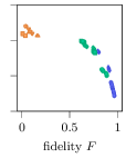
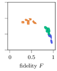
(b) VQE, w/o (left) and w/ (right) dynamical decoupling.

Figure 20: Fidelity $F$ versus relative error $E$ for the QAOA and VQE circuits with $L=1$ layer for all LamA use case examples executed on ibmq_ehningen. The results stem from the same experiment as described in Figure 15. The legend for the marker symbols can be found in Figure 19.

Metrics to predict quality

In the upper paragraph we have seen that the quality of the quantum computer results strongly differ for the different examples but also for different transpilations of the same example, see for example Figure 15 and in particular the variances for each example. Thus, an interesting question is wether we can predict the expected quality (for example in terms of the fidelity) from the transpiled quantum circuits.

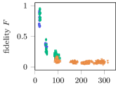
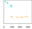
(a) QAOA, w/o dynamical decoupling, ibmq_ehningen (left), simulator with noise model (right).

(b) VQE, w/o dynamical decoupling, ibmq_ehningen (left), simulator with noise model (right).

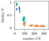
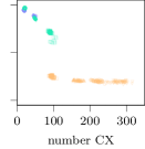
(c) QAOA, w/ dynamical decoupling, ibmq_ehningen (left), simulator with noise model (right).

(d) VQE, w/ dynamical decoupling, ibmq_ehningen (left), simulator with noise model (right).

Figure 21: Number of $\operatorname{CX}$ gates versus fidelity $F$ for the QAOA and VQE circuits with $L=1$ layer for all LamA use case examples executed on ibmq_ehningen and on a simulator with the noise model of ibmq_ehningen. The results stem from the same experiment as described in Figure 15. The noise model is built with the calibration data from the time when the circuits ran on ibmq_ehningen. The legend for the marker symbols can be found in Figure 19.

As we have seen above, the $\operatorname{CX}$ gate is by far the most erroneous hardware gate. Consequently, a simple metric to assess a quantum circuit is to count the number of $\operatorname{CX}$ gates of the transpiled version of the circuit. In Figure 21 we show the number of $\operatorname{CX}$ gates versus the fidelity $F$ for all our LamA examples for both QAOA and VQE on ibmq_ehningen. Additionally, we provide the fidelities of a noisy simulator that is built with a noise model using the calibration data of ibmq_ehningen from the time when the circuits were executed on the real machine. We can make the following observations: First of all, we see for QAOA without dynamical decoupling (Figure 21(a)) a drastic drop of the fidelity with increasing number of $\operatorname{CX}$ gates. In fact, only the examples with around 20 $\operatorname{CX}$ gates (lama_0p1 and lama_1p1), show an acceptable fidelity, the examples with around 50 $\operatorname{CX}$ gates (lama_0p2 and lama_1p2) are already much worse, closely followed by the examples with around 100 $\operatorname{CX}$ gates (lama_1p3 and lama_2p1), and finally all examples with more than 150 $\operatorname{CX}$ (lama_2p2 – lama_2p4) give a fidelity around $0$. Also note that the simulation with the noise model of the backend does hardly agree with the real results. In particular, note the strong differences for examples series lama_0p* and lama_1p*. For QAOA with dynamical decoupling (Figure 21(c)) we see an improvement in particular for lama_0p2 and lama_1p2 (both around 50 $\operatorname{CX}$ gates). Also note that the fidelities of lama_1p3 and lama_2p1 (both around 100 $\operatorname{CX}$ gates) now differ stronger and come closer to the predicted gap of the simulation. Here, we see the effect of the number of qubits of the different example series (recall lama_1p* uses 8 and lama_2p* uses 16 qubits). The effect of the qubit number is more drastically seen in the VQE experiments (Figures 21(b) and 21(d)). Although the number of $\operatorname{CX}$ gates is nearly the same the fidelities for example series lama_0p* is better than for example series lama_1p*, and both are much better than for example series lama_2p*. As for QAOA we also observe improvements when using dynamical decoupling and that simulations and real experiments do not match well.

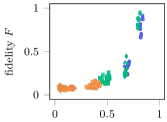
(a) QAOA, w/o dynamical decoupling, ibmq_ehningen (left), simulator with noise model (right).

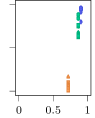
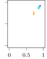
(b) VQE, w/o dynamical decoupling, ibmq_ehningen (left), simulator with noise model (right).

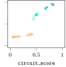
(c) QAOA, w/ dynamical decoupling, ibmq_ehningen (left), simulator with noise model (right).

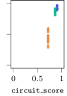
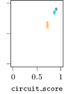
(d) VQE, w/ dynamical decoupling, ibmq_ehningen (left), simulator with noise model (right).

Figure 22: circuit_score, as defined in Algorithm 1, versus fidelity $F$ for the QAOA and VQE circuits with $L=1$ layer for all LamA use case examples executed on ibmq_ehningen and on a simulator with the noise model of ibmq_ehningen. The results stem from the same experiment as described in Figure 15. The noise model is built with the calibration data from the time when the circuits ran on ibmq_ehningen. The legend for the marker symbols can be found in Figure 19.

As we have seen, the number of $\operatorname{CX}$ gates is not able to accurately predict the fidelity. In particular, we observed that circuits with the same number of $\operatorname{CX}$ gates can result in strongly different fidelities. In these cases the assumption is obvious that the circuits use different qubits of ibmq_ehningen as all qubits and the gates, that are executed on them, all have with different error rates. A metric that incorporates the errors of the quantum gates is for example presented in [54, Algorithm 1]. We use it in the form of the circuit_score as given in Algorithm 1, where we include besides the quantum gates also the measurement in the instructions set $\{G\}$. Note that a circuit_score $\approx 1$ indicates a circuit with high quality instructions, whereas circuit_score $\approx 0$ hints at a circuit with low fidelity instructions.

1:Input: transpiled circuit with instructions $\{G\}$, error map $\mathcal{E}$

2:circuit_score $\leftarrow$ 1

3:for $g\in\{G\}$ do

4:     circuit_score $\leftarrow$ circuit_score $\ast$ $(1-\mathcal{E}(g))$

5:end for

6:return circuit_score

Algorithm 1 Algorithm for circuit_score

In Figure 22 we report the same experiments as for Figure 21 but with the circuit_score instead of the number of $\operatorname{CX}$ gates. In general, we make the same observations we already did for the number of $\operatorname{CX}$ gates. In particular, we see that also the circuit_score is in many cases not able to accurately predict the fidelity, see for example the individual transpilations of lama_0p1 and lama_1p1 in Figure 22(a), which have approximately the same circuit_score but their fidelity differs strongly. The same holds for the different transpilations of lama_0p2 and lama_1p2. Only the fidelities of lama_1p3 and lama_2p1 can be distinguished a bit better using the circuit_score than compared to the number of $\operatorname{CX}$ gates. Also note that, by construction, the circuit_score cannot reveal the effect of dynamical decoupling as can be seen by comparing Figure 22(a) with Figure 22(c) or Figure 22(b) with Figure 22(d). Moreover, the circuit_score does not incorporate the number of qubits so it cannot by used to compare examples with different qubit numbers. This is prominently seen in the VQE results in Figures 22(b) and 22(d), where the circuits all have a similar circuit_score but the fidelities differ strongly.

Reproducibilty over time

The error rates of today’s quantum computers are not constant but change over time. Thus, it is interesting how the results of our experiments look at different days. In Figure 23 we report on the fidelity for lama_1p2 on four different dates. For QAOA without dynamical decoupling (Figure 23(a)) we see that the median fidelity is nearly constant over the four days but the variance of the 75 different transpilations differs. For QAOA with dynamical decoupling (Figure 23(c)) the results look different. In particular, the median fidelity as well as the the distribution of the fidelities of the different transpilations differ strongly over the four days. For example, on 2023/10/17 and 2023/10/26 we see a more or less uniform distribution around the median, whereas on 2023/10/18 we see two clusters – one around a high fidelity and one around a low one. For VQE (Figures 23(b) and 23(d)) there are far less deviations in the four days, in particular in the case with dynamical decoupling.

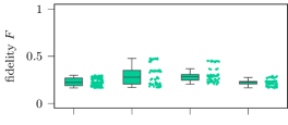
(a) QAOA, w/o dynamical decoupling.

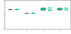
(b) VQE, w/o dynamical decoupling.

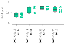
(c) QAOA, w/ dynamical decoupling.

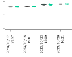
(d) VQE, w/ dynamical decoupling.

Figure 23: Fidelity $F$ for the QAOA and VQE circuits with $L=1$ layer for lama_1p2 executed on ibmq_ehningen on different dates. The experiment setup as is the same as described in Figure 15.

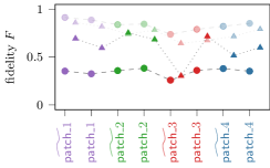
(a) 2023/10/27 20:38.

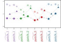
(b) 2023/11/22 18:22.

Figure 24: Fidelity $F$ for the QAOA circuit with $L=1$ layer for lama_0p2 executed on different qubit patches of ibmq_ehningen on two different dates. In all $\widetilde{\textsf{patch}\_\textsf{i}}$ there is a qubit triplet (marked in bold and underlined in the legend) that suffers from cross talk. In $\textsf{patch}\_\textsf{i}$ one qubit is exchanged such that these patches do not contain a cross talk triplet. As shown in the legend the marker type indicates wether dynamical decoupling was used in the quantum circuit. The transparent markers stem from a simulation of the quantum circuits using a simulator with the noise model of ibmq_ehningen. The noise model is built with the calibration data from the time when the circuits ran on ibmq_ehningen.

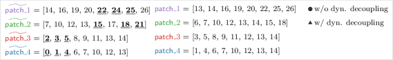
(a) 2023/10/27 20:18

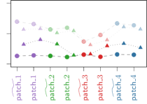
(b) 2023/11/22 18:40

Figure 25: Fidelity $F$ for the QAOA circuit with $L=1$ layer for lama_1p3 executed on different qubit patches of ibmq_ehningen on two different dates. The setup is the same as for Figure 24.

Choice of best qubits and cross talk

We have seen in the upper experiments that different transpilations of the same example (i.e. of the same logical QAOA or VQE circuit) can lead to drastically different fidelities. With the number of $\operatorname{CX}$ gates and the circuit_score we considered two metrics to explain this behavior, but both were not able to distinguish good from bad transpilations. Clearly, the question arises if the different fidelities stem from error sources that are not covered by these two metrics. One candidate for this error source is cross talk. This phenomenon has been analyzed in [55] for ibmq_ehningen and the qubit triplets that suffer from it have been identified. Using this information we want to analyze if cross talk is responsible for the lower fidelities we see in our experiments. For this we chose four cross talk qubit triplets of ibmq_ehningen, namely [0, 1, 4], [2, 3, 5], [15, 18, 21], and [22, 24, 25]. Then, we selected four patches of the quantum processor that contain these qubit triplets. We name these patches $\widetilde{\textsf{patch}\_1}$, …, $\widetilde{\textsf{patch}\_4}$. Afterwards, we exchanged a single qubit in each of these patches so that the cross talk qubit triplet is no longer part of the patch. We call these patches $\textsf{patch}\_1$, …, $\textsf{patch}\_4$. We did this procedure for patches of sizes 6 and 8 qubits. Having these patches of the quantum processor we transpiled the logical QAOA circuit for lama_0p2 and for lama_1p3 10 times and gave the transpiler our patches as initial layout. We set the optimization_level to 3 so that we get optimized circuits. From the resulting transpilations we removed those where the optimization of the transpiler changed the qubits. We ran the remaining circuits on ibmq_ehningen on two different dates. In Figures 24 and 25 we report the mean of the fidelities for lama_0p2 and for lama_1p3, respectively. For QAOA without dynamical decoupling (indicated by the circle markers) we see no (Figure 25) or only a slight (Figure 24) difference between the cross talk and non cross talk patches. In particular, in Figure 24(b) we see a better fidelity in the non cross talk patches. Considering the circuit with dynamical decoupling (triangle markers) we observe large differences for the different patches. More precisely, we see for both lama_0p2 and lama_1p3 a better fidelity for the non cross talk patch $\textsf{patch}\_3$ compared to its counterpart $\widetilde{\textsf{patch}\_3}$ with the cross talk triplet. For lama_0p2 (Figure 24) the difference is drastic. However, for $\textsf{patch}\_2$ and $\widetilde{\textsf{patch}\_2}$ the situation is the other way round (at least for Figures 24(a), 25(a), and 25(b)). Here, the cross talk patches yield a better fidelity. For the other patches there are either no big differences, the cross talk patch is a bit better ($\textsf{patch}\_1$ and $\widetilde{\textsf{patch}\_1}$ in Figure 24(a)), or the non cross talk patch is a bit better ($\textsf{patch}\_4$ and $\widetilde{\textsf{patch}\_4}$ in 24(b)). Thus, we conclude that cross talk might be one of the error sources leading to the variance in fidelities, that we see in our experiments, but is not the only missing error source in a metric to explain the fidelity.

4.3 Experiments on ibm_cairo, ibm_sherbrooke, and ibm_torino

In this section we present the same experiments that we ran on ibmq_ehningen in Section 4.2 for the backends ibm_cairo, ibm_sherbrooke, and ibm_torino. As it can be seen in Table 1 the first has the same processor type as ibmq_ehningen, the second one is a 127 qubit processor from 2022, and the last is the newest processor available from IBM and has 133 qubits. This choice lets us, on the one hand, compare two similar processors and, on the other hand, enables us to show and assess the technological progress over the last years.

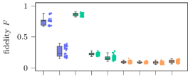
(a) QAOA, w/o dynamical decoupling.

(b) VQE, w/o dynamical decoupling.

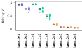
(c) QAOA, w/ dynamical decoupling.

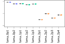
(d) VQE, w/ dynamical decoupling.

Figure 26: Fidelity $F$ obtained from executing the QAOA (left) and VQE (right) circuits with $L=1$ layer for all LamA use case examples on ibm_cairo. The experiment setup is the same as described in Figure 15. The fist job of the session ran on 2023/12/13 11:44.

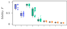
(a) QAOA, w/o dynamical decoupling.

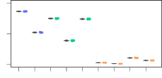
(b) VQE, w/o dynamical decoupling.

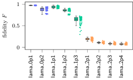
(c) QAOA, w/ dynamical decoupling.

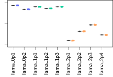
(d) VQE, w/ dynamical decoupling.

Figure 27: Fidelity $F$ obtained from executing the QAOA (left) and VQE (right) circuits with $L=1$ layer for all LamA use case examples on ibm_sherbrooke. The experiment setup is the same as described in Figure 15. The fist job of the session ran on 2023/12/15 10:05.

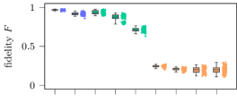
(a) QAOA, w/o dynamical decoupling.

(b) VQE, w/o dynamical decoupling.

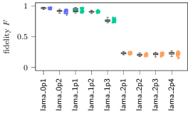
(c) QAOA, w/ dynamical decoupling.

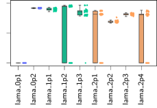
(d) VQE, w/ dynamical decoupling.

Figure 28: Fidelity $F$ obtained from executing the QAOA (left) and VQE (right) circuits with $L=1$ layer for all LamA use case examples on ibm_torino. The experiment setup is the same as described in Figure 15. The fist job of the session ran on 2023/12/11 13:03.

Metrics to predict quality

Let us start with showing the fidelities for all LamA examples. In Figure 26 we show them for ibm_cairo, in Figure 27 for ibm_sherbrooke, and in Figure 28 for ibm_torino. As expected, we do not see major differences when comparing the results of ibm_cairo with those of ibmq_ehningen, recall Figure 15. The most notable difference is that the VQE fidelities have a much smaller variance for ibm_cairo. This can also be observed by comparing the VQE fidelities of ibm_sherbrooke with ibmq_ehningen. Surprisingly, we can also observe that without dynamical decoupling the fidelities for lama_0p2 and lama_1p2 are quite a bit lower for ibm_sherbrooke than for ibmq_ehningen. Looking at QAOA we see larger variances on ibm_sherbrooke in the case without dynamical decoupling, in particular for lama_1p2. When using dynamical decoupling we see an improvement in comparison to ibmq_ehningen, particularly for the smaller example series lama_0p* and lama_1p*. Last, for QAOA and ibm_torino we see a significant improvement in the fidelities. Indeed, all fidelities in example series lama_0p* and lama_1p* are drastically improved and in many examples near to $1$. But also the fidelities of the largest examples in example series lama_2p* are higher, which could not be achieved by the other backends. For the VQE circuits we see many outliers from unclear error sources. However, for the other circuits we again see drastically higher fidelities in comparison to ibmq_ehningen and also compared to the other backends considered in this paper.

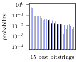
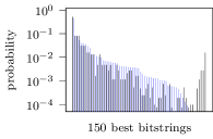
(a) QAOA, lama_0p2.

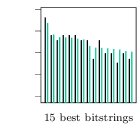
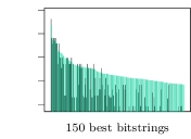
(b) QAOA, lama_1p3.

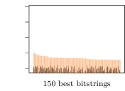
(c) QAOA, lama_2p3

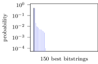
(d) VQE, lama_0p2.

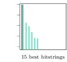
(e) VQE, lama_1p3.

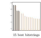
(f) VQE, lama_2p3.

Figure 29: Probabilities resulting from executing the QAOA (top) and VQE (bottom) circuits with $L=1$ layer for different LamA use case examples on ibm_torino (colored bars) and on an exact simulator (black bars). The experiment setup is the same as described in Figure 16.

As we have seen the most differences in comparison to ibmq_ehningen are obtained from ibm_torino. Thus, we restrict ourselves to show here the probability distributions and the relative error for this backend. In Figure 29 we show the probability distributions $\{\widetilde{p}_{\mathbf{b}}\}$ from ibm_torino with the same setting as we had in Figure 16 for ibmq_ehningen. For QAOA and lama_0p2 as well as lama_1p3 we see a higher probability for the best bitstring and a high agreement of the best 15 bitstrings for ibm_torino. Moreover, we see a faster decay of the probability of the bitstrings that should have zero probability according to the exact simulation. Only for lama_2p3 and QAOA we do only observe a very small improvement. On the contrary, we observe for all VQE examples probability distributions from ibm_torino that match with the exact simulation fairly well. The most significant improvement can be seen for lama_2p3 which matches well with the improved fidelity we have seen in Figure 28 above.

Last in this paragraph, we plotted in Figure 30 the relative error $E$ for ibm_torino. Comparing with the error of ibmq_ehningen, see Figure 18, we see that the results are much closer to the simulation for QAOA. This is also true for VQE except of the outliers that we already saw in Figure 28.

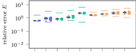
(a) QAOA, w/o dynamical decoupling.

(b) VQE, w/o dynamical decoupling.

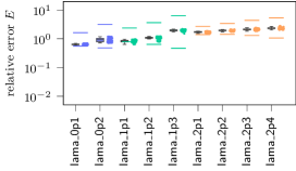
(c) QAOA, w/ dynamical decoupling.

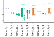
(d) VQE, w/ dynamical decoupling.

Figure 30: Relative error $E$ obtained from executing the QAOA (left) and VQE (right) circuits with $L=1$ layer for all LamA use case examples on ibm_torino. The experiment setup is the same as described in Figure 16. The lower horizontal lines indicate the relative error when using an exact simulator instead of ibm_torino. The upper lines stem from the mean of the relative error of the probability distributions of 50 random statevectors.

Metrics to predict quality

We conclude the LamA use case section by reporting on metrics to predict the fidelity. For ibmq_ehningen we considered the number of $\operatorname{CX}$ gates and the circuit_score. These two metrics can also be used for ibm_cairo. However, ibm_sherbrooke and ibm_torino do not have the $\operatorname{CX}$ gate as two qubit hardware gate but the $\operatorname{ECR}$ and the $\operatorname{CZ}$ gate, respectively. For both backends the two qubit hardware gate is the most erroneous so that they play the analog role (and can be used as the analog metric) as the $\operatorname{CX}$ gate for ibmq_ehningen. By definition the circuit_score is computed from the transpiled circuits and thus the different hardware gates enter automatically there.

In Figures 31, 32, and 33 we show the two metrics versus the fidelity $F$ for ibm_cairo,
ibm_sherbrooke, and ibm_torino, respectively. The results for ibmq_ehningen are given in Figure 21 for the number of $\operatorname{CX}$ gates and in Figure 22 for the circuit_score. Note that for the other backends we are not showing simulations with noise models of the backends. Comparing the results from ibm_cairo with ibmq_ehningen we see very similar fidelities for QAOA. Only for lama_1p3 and in the case with dynamical decoupling ibm_cairo achieves a bit higher fidelities. Note that this improvement is not represented by the circuit_score. For the VQE circuits we observe better fidelities from ibmq_ehningen and, again, note that neither the number of $\operatorname{CX}$ gates nor the circuit_score can reflect this difference. Next, let us compare ibm_sherbrooke and ibmq_ehningen. Most prominently, we see that ibm_sherbrooke yields, for the same number of two qubit gates or the same circuit_score, fidelities with a much larger variance than ibmq_ehningen. Other than that the observations we did with ibm_cairo also hold for this backend. For ibm_torino the fidelities look quite different than for the other three backends. In particular, we see high fidelities for example series lama_0p* and lama_1p* and that the number of $\operatorname{CZ}$ gates or the circuit_score can predict well the decrease of the fidelity for the different examples. However, note that for QAOA the fidelities of lama_2p1 are much lower than for lama_1p3 although the circuits have the same number of $\operatorname{CZ}$ gates and nearly the same circuit_scores. Here, we see that the different number of qubits (and the associated error sources) are not well represented by neither of our two metrics. Last, note that all examples of lama_2p*, and in particular in the cases with dynamical decoupling, have fidelity values on a plateau of around $0.22$ although they have strongly different numbers of $\operatorname{CZ}$ gates and circuit_scores.

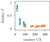
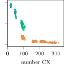
(a) QAOA, w/o (left) and w/ (right) dynamical decoupling.

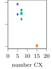
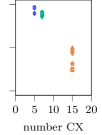
(b) VQE, w/o (left) and w/ (right) dynamical decoupling.

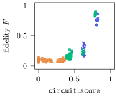
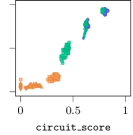
(c) QAOA, w/o (left) and w/ (right) dynamical decoupling.

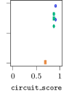
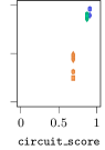
(d) VQE, w/o (left) and w/ (right) dynamical decoupling.

Figure 31: Number of $\operatorname{CX}$ gates (top) and circuit_score (bottom) versus fidelity $F$ for the QAOA and VQE circuits with $L=1$ layer for all LamA use case examples executed on ibm_cairo. The results stem from the same experiment as shown in Figure 26. The legend for the marker symbols can be found in Figure 19.

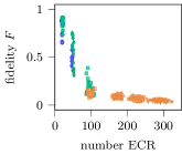
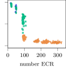
(a) QAOA, w/o (left) and w/ (right) dynamical decoupling.

(b) VQE, w/o (left) and w/ (right) dynamical decoupling.

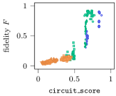
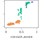
(c) QAOA, w/o (left) and w/ (right) dynamical decoupling.

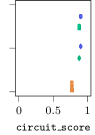
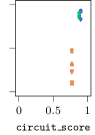
(d) VQE, w/o (left) and w/ (right) dynamical decoupling.

Figure 32: Number of $\operatorname{ECR}$ gates (top) and circuit_score (bottom) versus fidelity $F$ for the QAOA and VQE circuits with $L=1$ layer for all LamA use case examples executed on ibm_sherbrooke. The results stem from the same experiment as shown in Figure 27. The legend for the marker symbols can be found in Figure 19.

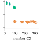
(a) QAOA, w/o (left) and w/ (right) dynamical decoupling.

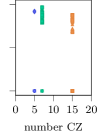
(b) VQE, w/o (left) and w/ (right) dynamical decoupling.

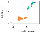
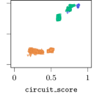
(c) QAOA, w/o (left) and w/ (right) dynamical decoupling.

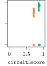
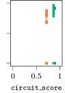
(d) VQE, w/o (left) and w/ (right) dynamical decoupling.

Figure 33: Number of $\operatorname{CZ}$ gates (top) and circuit_score (bottom) versus fidelity $F$ for the QAOA and VQE circuits with $L=1$ layer for all LamA use case examples executed on ibm_torino. The results stem from the same experiment as shown in Figure 28. The legend for the marker symbols can be found in Figure 19.

4.4 Experiments on D-Wave Advantage 4.1

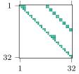
(a) lama_3p1

(b) lama_3p2

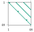
(c) lama_4p1

(d) lama_4p2

Figure 34: Sparsity of QUBO matrix $\mathbf{Q}$ for example series lama_3p* and lama_4p*.

This last section of the LamA use case is dedicated to experiments on the quantum annealer D-Wave Advantage 4.1. Recall from Table 2 that this quantum system has more than 5000 qubits. Thus, we consider in this section, besides the previously introduced example series, two additional example series termed lama_3p* and lama_4p*. Both series model one charging station with four charging levels and $T=8$ time slots. In lama_3p* we have the case of $K=2$ cars, while in lama_4p* we have $K=3$. This results in QUBOs with 32 and 48 variables, respectively. In both series we consider two examples, where in the first example the time slots, when the different cars charge energy, only overlap in one time slot, while in the second one the overlap extends for all available slots. As a consequence the respective first example is only weakly coupled, while the second one has a strong coupling between the variables. This can nicely be seen in the sparsity plots in Figure 34.

example	# logical qubits	# physical qubits	# chains	max chain length
lama_0p1	6	6	0	0
lama_0p2	6	8	2	2
lama_1p1	8	8	0	0
lama_1p2	8	10	2	2
lama_1p3	8	12	4	2
lama_2p1	16	16	0	0
lama_2p2	16	23	7	2
lama_2p3	16	27	10	3
lama_2p4	16	32	16	2
lama_3p1	32	32	0	0
lama_3p2	32	98	32	4
lama_4p1	48	65	17	2
lama_4p2	48	192	48	5

Table 4: The number of logical qubits, required physical qubits, number of chains, and maximum chain length for all LamA use case examples.

As we have discussed in Section 3.2 our logical QUBOs have to be embedded onto the QPU. In Table 4 we give the details on the amount of utilized physical qubits, chains, and the maximum chain lengths for all LamA use case examples. Note that in most cases more physical qubits are needed than the problem has logical ones. This is due to the need for chains, which are required to overcome the limited hardware connectivity in correctly representing the coupling of QUBO variables. We visualize this in Figure 35 exemplary for the embeddings of the examples lama_0p2, lama_1p3, and lama_2p4. It is instructive to compare these plots with the sparsity pattern of the QUBO matrices given in Figure 6. For example, we can see that lama_0p2 is mapped to the Pegasus unit cell, recall Figure 4, by directly embedding 4 logical qubits onto 4 physical qubits, while representing the remaining 2 logical qubits with 2 chains containing 2 physical qubits each. Thus, the embedding of lama_0p2 requires 8 physical qubits although the underlying QUBO only has 6 (logical) qubits. By this reasoning, we see that lama_1p3 and lama_2p4 require 12 and 32 physical qubits, respectively, to embed their 8 and 16 logical qubits.

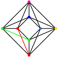
(a) lama_0p2.

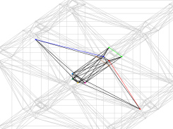
(b) lama_1p3.

(c) lama_2p4.

Figure 35: Embedding of the QUBO matrix $\mathbf{Q}$ of different LamA examples onto D-Wave Advantage 4.1. The colored lines are chains, the black lines are hardware connections, and the gray lines are couplers which are not used in the embedding.

Besides the embedding we pointed out in Section 3.2 that the hardware parameters chain strength and anneal time can have a strong impact on the quality of the annealing solution. In the next paragraphs we report on experiments that illuminate this. In order to obtain statistically relevant results, we ran each experiment 10 times. For each such run we used either 400 or 1000 reads. We report on the quality of the D-Wave results in terms of the percentage of feasible and optimal solutions from the overall reads. Here, a bitstring is called feasible if it satisfies the constraint (2b) of our underlying optimization problem. This is understood in the sense that the integer vector stemming from the bitstring’s transformation via the transformation matrix (2b) satisfies the constraint.

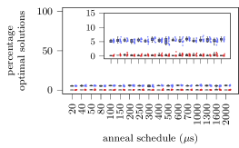
Figure 36: Percentage of feasible (left) and optimal (right) solutions for different anneal schedules for lama_0p1 (blue markers) and lama_4p2 (crimson markers). For the former the chain strength was chosen as 0.3 and for the latter as 0.8. For each run we used 400 reads.

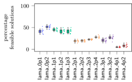
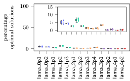
Figure 37: Percentage of feasible (left) and optimal (right) solutions for all LamA examples. The anneal schedule was chosen as 300 $\mu$s. For each run we used 400 reads.

Anneal schedule

We systematically studied the effect of the anneal schedule and of the chain strength for all examples in the LamA use case. Thereby, we observed an almost constant quality of the solutions with respect to the anneal time. We show this exemplarily for lama_0p1 and lama_4p2 in Figure 36. Since the precise choice of the annealing schedule is only secondary for our LamA examples we fixed it to 300 $\mu$s and report the solutions qualities in Figure 37. There, we can nicely see how the percentages of feasible and optimal solutions decrease when the problem size increases.

Chain strength

In contrary to the anneal schedule, we observe an impact of the chain strength in the quality of our annealing solutions. For example, we see in Figure 38(b) that for lama_0p2 a higher chain strength decreases the fraction of both feasible and optimal solutions. For lama_1p2 and lama_1p3 in Figures 38(d) and 38(e), respectively, we first observe a fast increase in quality with increasing anneal time until a certain threshold and afterwards a slow decline. The same behavior can be seen for lama_2p4, lama_3p2, and lama_4p2 in Figures 38(i), 39(b), and 39(d), respectively. These are exactly the examples with the strongest coupling. Recalling how these problems have to be embedded onto the QPU it is clear that they are most sensitive to the chain strength. Last, let us note the decrease in the fraction of feasible solutions from around 50 percent in lama_0p* to only a few percent in lama_4p*. The same holds for the percentage of optimal solutions. Here, we can clearly observe the limitations of current quantum hardware when dealing with large problems.

(a) lama_0p1.

(b) lama_0p2.

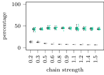
(c) lama_1p1.

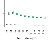
(d) lama_1p2.

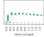
(e) lama_1p3.

(f) lama_2p1.

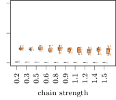
(g) lama_2p2.

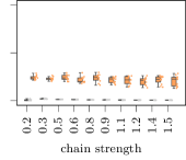
(h) lama_2p3.

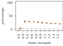
(i) lama_2p4.

Figure 38: Percentage of feasible (colored markers) and optimal (gray markers) solutions for different chain strength values for example series lama_0p* (first row), lama_1p* (second row), and lama_2p* (third and fourth row). The anneal time was chosen as 300 $\mu$s and for each run we used 1000 reads.

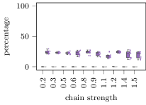
(a) lama_3p1.

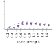
(b) lama_3p2.

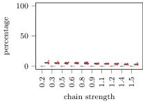
(c) lama_4p1.

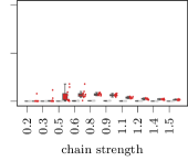
(d) lama_4p2.

Figure 39: Percentage of feasible (colored markers) and optimal (gray markers) solutions for different chain strength values for example series lama_3p* (first row) and lama_4p* (second row). The anneal time was chosen as 300 $\mu$s and for each run we used 1000 reads.

5 Use Case 2: Optimization of Truck Routes

In the truck routing problem (TRP) we aim to find the route with the shortest travel distance between a given set of cities. This route has to start and to end in a particular city (which is usually the depot of the truck) and each city may be visited only once on the route. The TRP, notorious for its NP-hard complexity, represents a significant challenge in combinatorial optimization. Finding the shortest route to visit every city once becomes exponentially harder as the number of cities increases (combinatorial explosion), rendering traditional algorithms inefficient. Thus, it is interesting to explore other paradigms to solve this problem. The formulation of the TRP as a QUBO problem opens the door for its representation on D-Wave systems. We will explore how to represent the TRP using the binary quadratic model (BQM), which is suitable for D-Wave’s QPU.

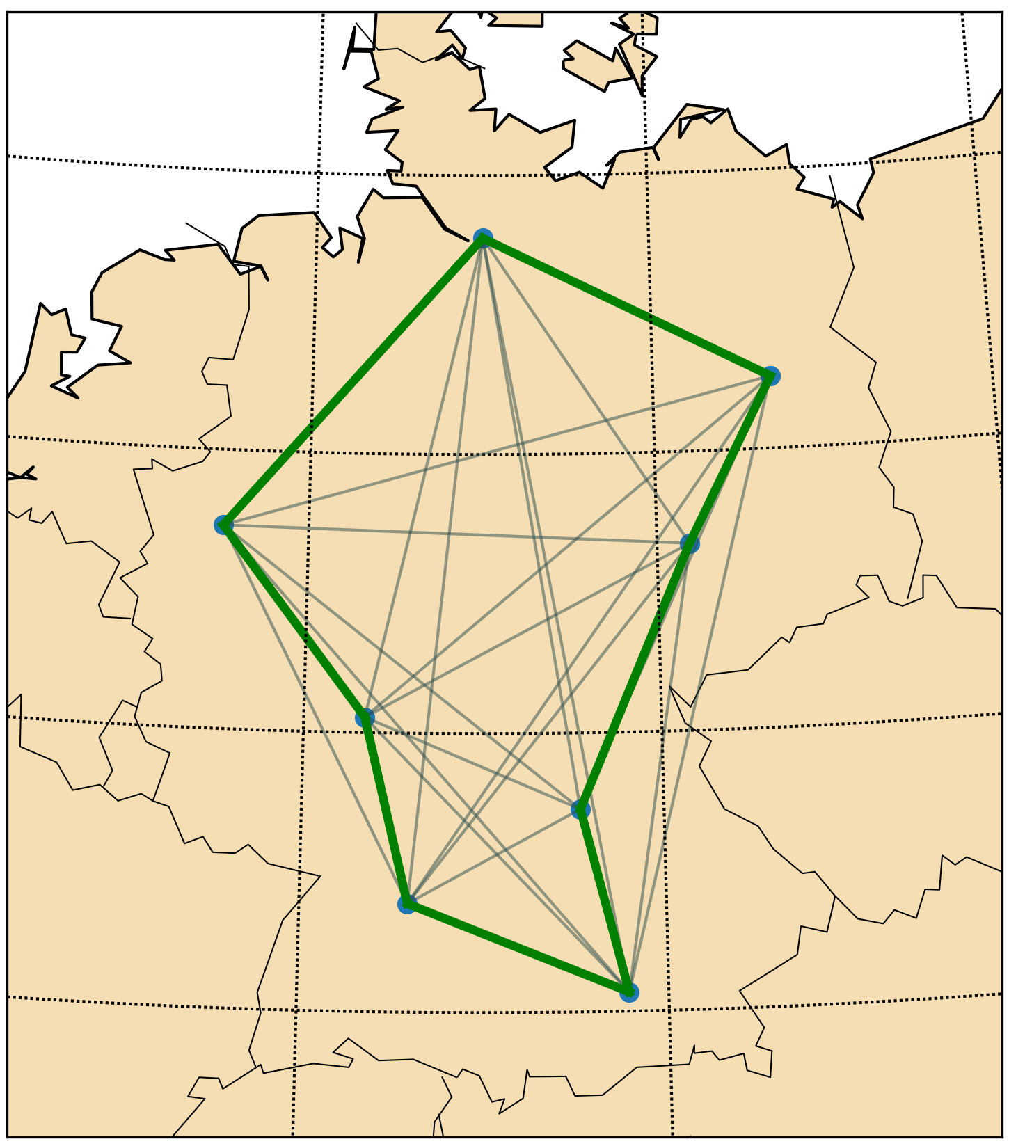
(a) Asymmetrical (a-trp_8).

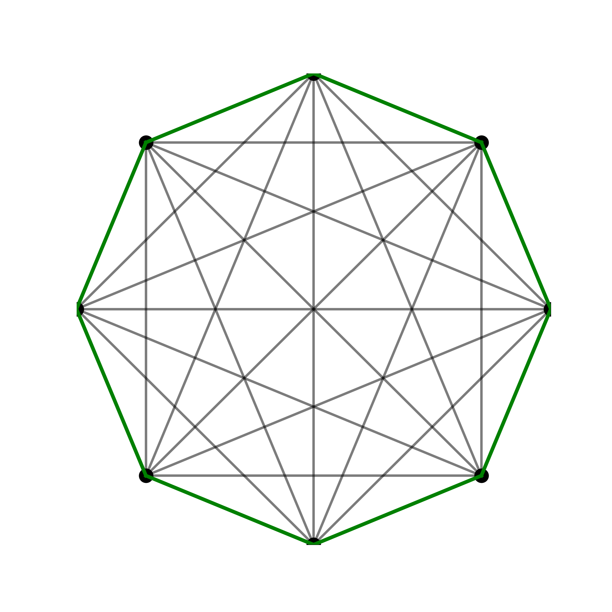
(b) Symmetrical (s-trp_8).

Figure 40: Examples for the two types of distributions that we consider in this paper: asymmetrical a-trp_8 (left) and symmetrical (right).

5.1 Problem formulation

Consider a set of $n$ cities represented by indices from $1$ to $n$. Let $b_{i,t}\in\{0,1\}$ be a binary variable indicating whether city $i\in\{1,...,n\}$ is visited ($b_{i,t}=1$) or not ($b_{i,t}=0$) at each time $t\in\{1,...,n\}$.

The QUBO formulation consists of two parts. Let $E$ be the set of tuples that indicate if two cities are connected and let $d_{ij}$ denote their distances. The quadratic QUBO terms are then given by

$$Q_{d}=\sum_{(i,j)\in E}d_{ij}\sum_{t=1}^{n}b_{i,t}b_{j,t+1}\ .$$ (23)

This part of the QUBO encodes the distances. The constraints are included into the cost function via

$$Q_{c}=\varrho\cdot\left[\sum_{i=1}^{n}\left(1-\sum_{t=1}^{n}b_{i,t}\right)^{2}+\sum_{t=1}^{n}\left(1-\sum_{i=1}^{n}b_{i,t}\right)^{2}\right].$$

The first term imposes that in the overall route each city is only visited once while the second term favors solutions where each time step shows up exactly once. The combined QUBO problem with distance minimization and constraints can be expressed by

$$Q=Q_{d}+Q_{c}\ .$$ (24)

Since there are $n$ possible locations for $n$ time steps, we need $n^{2}$ variables that can represent all possible combinations of time and city.

In this paper, we considered three different problem sizes. Each problem size has two different distributions of the cities, with one being asymmetric and the other radially symmetric. The asymmetrical distribution refers to a scenario where cities are placed randomly, resulting in a unique distance between each pair of cities. This randomness introduces complexity to the optimization problem, presenting a more challenging scenario for solution algorithms. On the other hand symmetrical distribution implies that cities are equidistantly placed on a ring. This uniformity simplifies the optimization landscape, potentially leading to more straight-forward solutions. The asymmetric and symmetric distribution problem classes are referred as a-trp_$m$ and s-trp_$m$, respectively, where $m$ corresponds to number of cities. The asymmetric and symmetric distributions of 8 cities are given in Figure 40. By using (24) we can build QUBO matrices for our problems. Their sparsity patterns are given in the Figure 41. We observe that the problems are strongly coupled. Note that the symmetric and asymmetric problems have the same sparsity pattern.

5.2 Binary quadratic model

In order to implement the QUBO formulation on the quantum annealer, it has to be reformulated as a binary quadratic model (BQM), that ideally has the form of an Ising Hamiltonian native to the hardware architecture. For that, a simple variable transformation from $b_{i,t}\in\{0,1\}$ to $x_{i,t}\in\{-1,1\}$ is done, where the relationship between the variables is simply

$$b_{i,t}=\frac{1+x_{i,t}}{2}\leavevmode\nobreak\ ,$$

which results in

$$H=\sum_{i=1}^{n}h_{i}x_{i}+\sum_{i=1}^{n}\sum_{j=1}^{n}J_{ij}x_{i}x_{j}+c\leavevmode\nobreak\ .$$ (25)

The coefficients $h_{i}$ (bias) and $J_{ij}$ (coupling strength) are related to the linear and quadratic QUBO terms, respectively, and are modified by the variable transformation. The constant term $c$ can be disregarded.

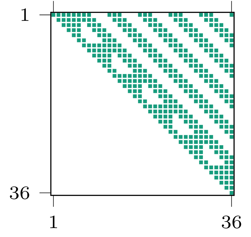
(a) a-trp_6 and s-trp_6.

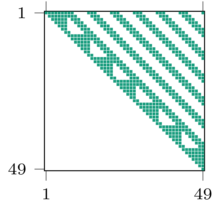
(b) a-trp_7and s-trp_7.

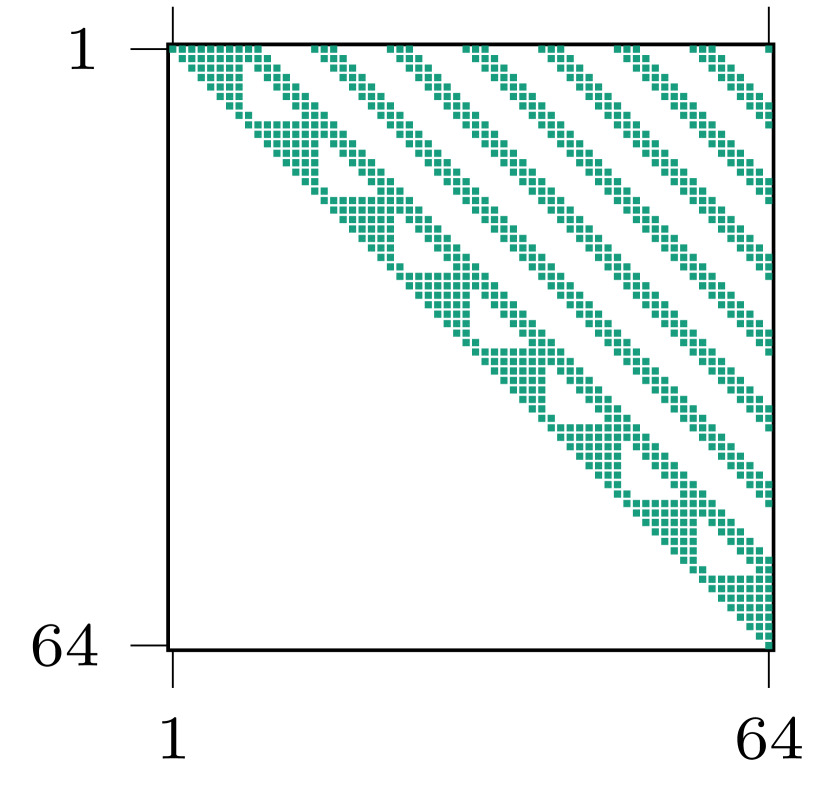
(c) a-trp_8 and s-trp_8.

Figure 41: Sparsity pattern of a QUBO matrix for 6, 7, and 8 cities.

5.3 Results

In this section, we present results of the TRP examples with respect to different hardware parameters. As in Section 4.4 we use the percentage of feasible and optimal solutions as quality metric. Feasible solutions are those which satisfy the constraints imposed in the QUBO problem and optimal solutions are feasible solutions with minimum distance traveled.

Setup

We used clique embedding [41, 56] to embed the the QUBO matrices onto the QPU Advantage 4.1. This method is particularly useful for the Pegasus chip when the source graph (QUBO graph) is a clique, i.e. a fully connected graph. D-Wave’s Ocean software provides a function, find_clique_embedding, which uses a polynomial-time algorithm to find better embeddings for cliques than the default embeddingcomposite method. We used CliqueSampler to solve the embeded problems. The strength lies in its specificity, rendering it unsuitable for general optimization problems lacking pronounced clique structures. An advantage of this type of method is that it tries to keep the maximum chain length low, which is beneficial for highly interconnected problems like the ones at hand.

Penalty parameters

We analyze two different penalty parameters effecting the quality of the solution. On the QUBO level we used $\varrho$ and on the hardware level the chian strength. The QUBO penalty parameter $\varrho$ controls the constraints in the problem formulation. The chain strength is responsible for keeping the chains consistent, penalizing chain breaks, and is implemented on a lower level concerning the actual Hamiltonian that describes the hardware operation. The number of anneal reads were 1500 for each combination of penalty and chain strength value. The heat map plot for the chain strength and the penalty parameter is instructive as these parameters ensure the integrity of the solution and the satisfaction of constraints. The percentage of feasible and optimal solutions for the asymmetrical distribution of cities are given in Figure 42. One common observation for all the different number of cities is that for small chain strength, quantum annealing almost cannot find any feasible solutions, irrespective of the strengths of penalty. In the case of a-trp_6, the chain strength of $0.6$ yields the highest percentage of solutions for nearly all penalties. On the contrary, the higher percentage of feasible solutions for a-trp_7 and a-trp_8 are obtained for chain strength of $0.9$ and only for larger penalty values. The problems a-trp_7 and a-trp_8 need to maintain the chain length of 6 and 7 to hold 284 and 436 physical qubits, respectively, see Table 5. Since the stronger chain strength can keep the longer chains and thus the original problem intact, they lead to higher percentages of feasible and optimal solutions. As the problem size increases the samller chain strength values fail to yield any solutions. Higher percentage of optimal solutions for a-trp_6 are obtained for the same values of chain strength values as for feasible solutions. On the other hand, for a-trp_7 and a-trp_8, stronger chain strengths and smaller penalty values yield optimal solutions. The higher percentage of feasible and optimal solutions do not share the same chain strength values. Overall, the percentage of feasible and optimal solutions reduces as we increase the problem size. In the case of symmetrical distribution of the cities, the percentage of feasible solutions for all cities is higher than in the asymmetrical distribution of cities, see Figure 43. For s-trp_6, with a chain strength of $0.6$ and for nearly all penalty values, we obtain the highest amount of feasible soultions. The same chain strength yields maximum optimal solutions. The feasible solutions for s-trp_7 are at maximum for higher chain strength values which is similar to the asymmetrical distribution of cities. On the contrary to the asymmetrical distribution, the same chain strength is enough to obtain a higher percentage of both feasible and optimal solution for s-trp_7 and s-trp_8.

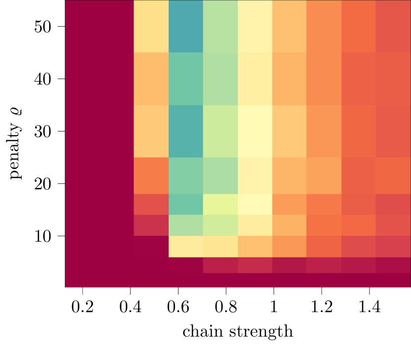
(a) a-trp_6.

(b) a-trp_7.

(c) a-trp_8.

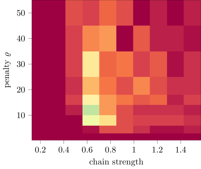
(d) a-trp_6.

(e) a-trp_7.

(f) a-trp_8.

Figure 42: Percentage of feasible (upper row) and optimal (lower row) solutions for asymmetrical distribution of cities with variable chain strength and penalty values. The number of anneal reads are 1500 for each combination of penalty and chain strength. The annealing time was chosen to be 300 $\mu$s. Clique embedding was used to embed the QUBO. The calculations were executed on Advantage 4.1 and results were obtained on 2023/11/06.

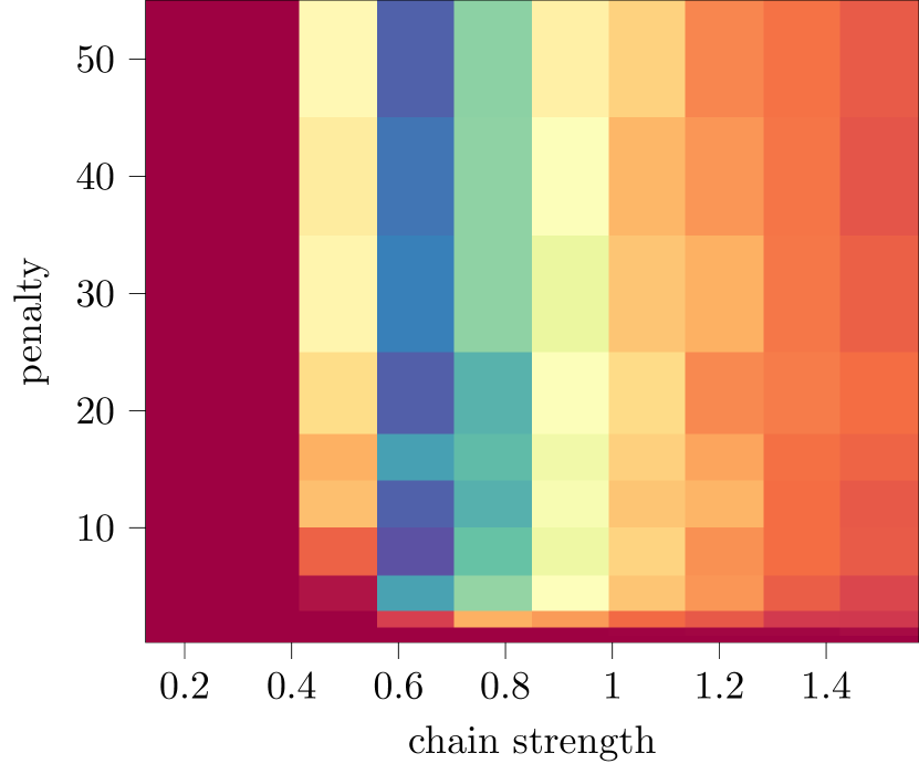
(a) s-trp_6.

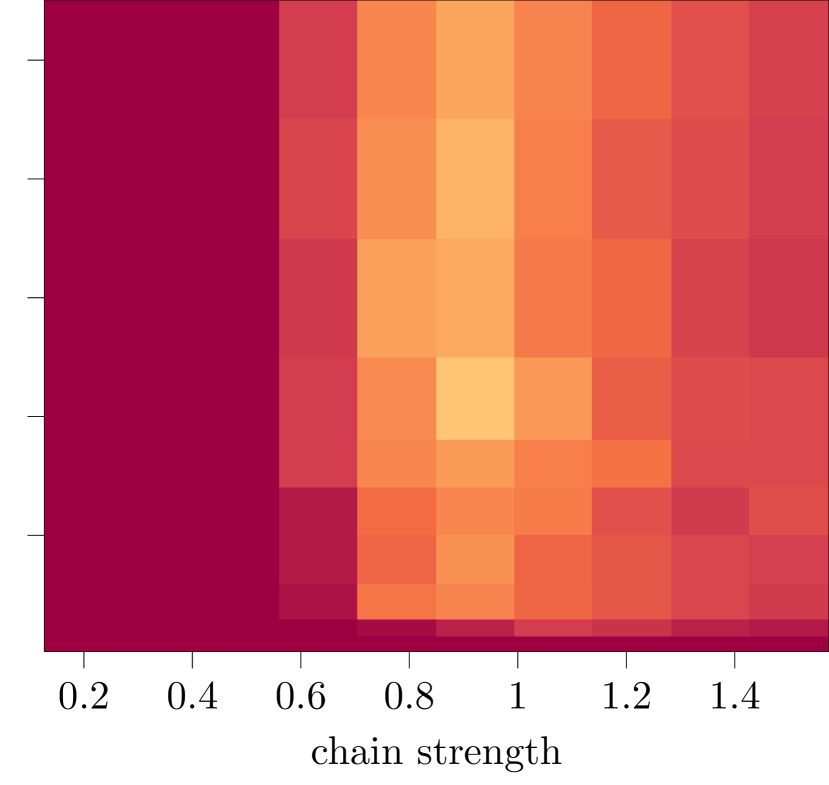
(b) s-trp_7.

(c) s-trp_8.

(d) s-trp_6.

(e) s-trp_7.

(f) s-trp_8.

Figure 43: Percentage of feasible (upper row) and optimal (lower row) solutions for symmetrical distribution of cities with variable chain strength and penalty values. The number of anneal reads are 1500 for each value of penalty and chain strength. The annealing time was chosen to be 300 $\mu$s. Clique embedding was used to embed the QUBO. The calculations were executed on Advantage 4.1 and results were obtained on 2023/11/11.

Anneal schedule

As we have discussed in Section 3.2, one of the most important parameters is the annealing time. Here, we discuss the impact of the annealing schedule on enhancing the likelihood of obtaining feasible and optimal solutions. We employed multiple anneal schedules for the annealing to observe the solution quality. Optimal values of chain strength and QUBO penalty were chosen from the heatmap analysis for all problem cases. Different anneal schedules were chosen from shorter times to longer times. We plotted the percentage of feasible and optimal solutions for asymmetric and symmetric distributions. Each marker in the Figures 44 and 45 corresponds to the percentage of feasible solutions for 400 anneal reads. There are 50 such markers for each anneal schedule resulting in total of $20000$ anneal reads. The feasible solutions for a-trp_6 has an inverted parabola type behavior, see Figure 44. Rapid annealing disrupts the system’s ability to maintain the ground state, leading to transitions to higher energy states associated with suboptimal or infeasible solutions. Conversely, longer anneal schedules beyond $600\,\mu s$ also reduce the percentage of feasible solutions, possibly due to factors like thermal relaxation or qubit noise. We observe the same beahviour in a-trp_7 but with a lesser intensity. For a-trp_8 the impact of the anneal schedule is not as significant as in the other cases. The inverted parabola behaviour is less pronounced in optimal solutions.

example	# logical qubits	# physical qubits	# of chains	chain length
a-trp_6, s-trp_6	36	172	36	5
a-trp_7, s-trp_7	49	284	49	6
a-trp_8, s-trp_8	64	436	64	7

Table 5: The number of logical qubits, physical qubits, chains, and chain length for all the problem sizes in the TRP use case. The symmetric and asymmetric problems have the same numbers.

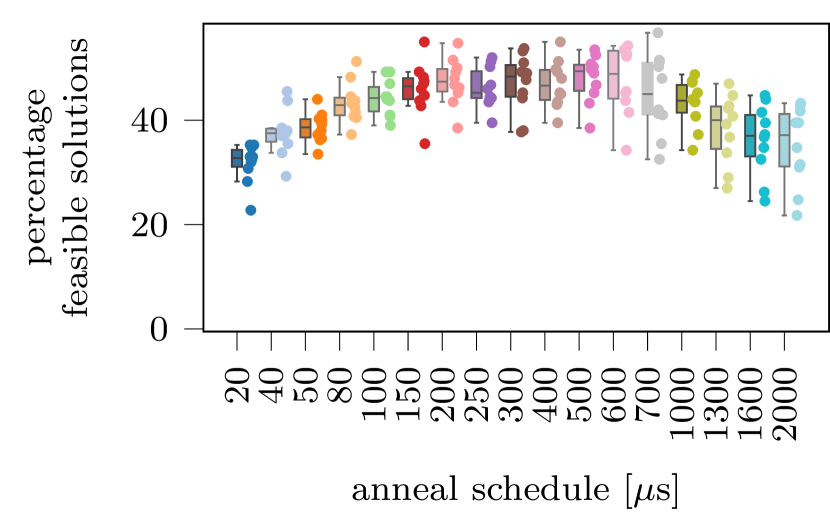
(a) a-trp_6.

(b) a-trp_7.

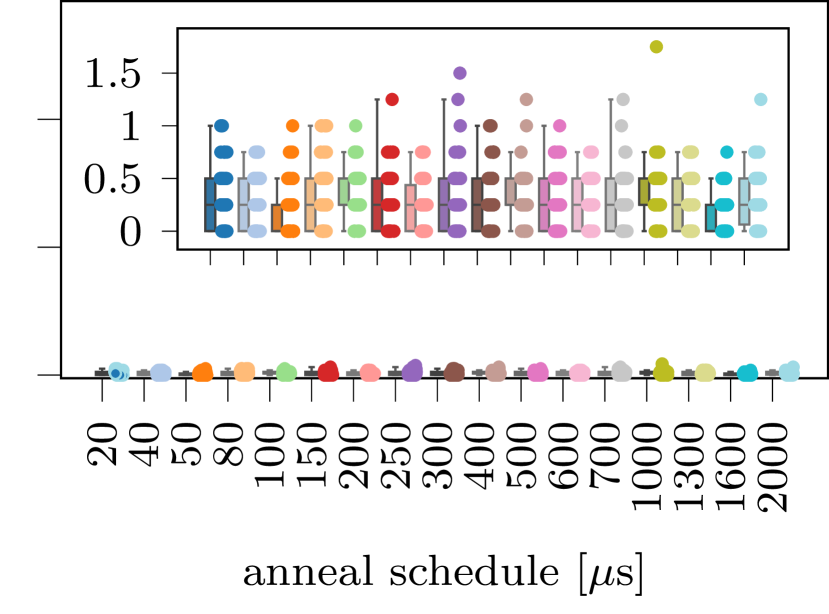
(c) a-trp_8.

(d) a-trp_6.

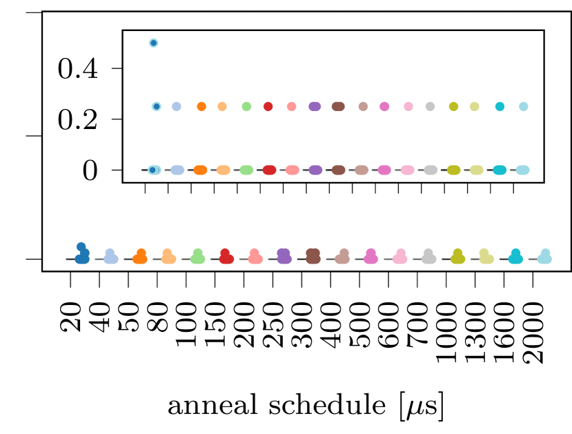
(e) a-trp_7.

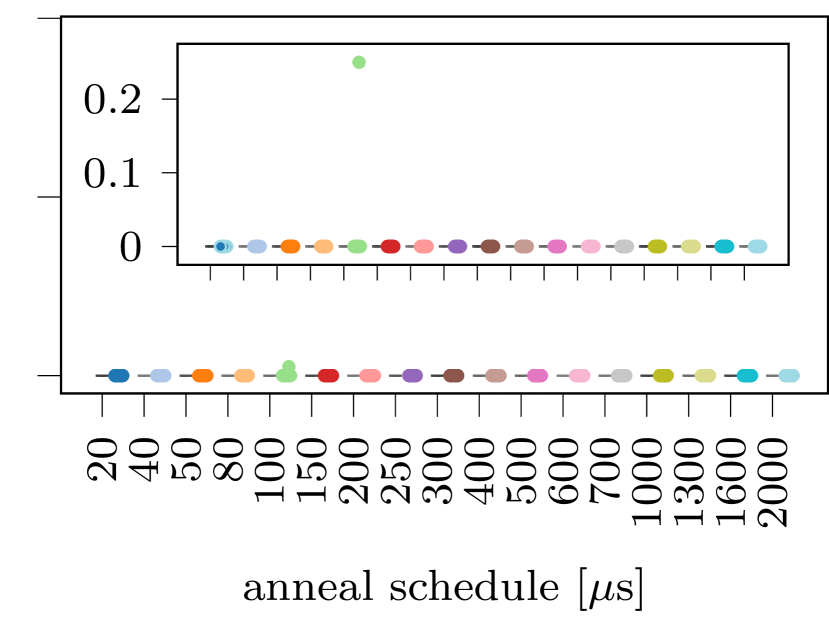
(f) a-trp_8.

Figure 44: Percentage of feasible and optimal solutions for asymmetrical distribution of cities with different anneal schedules. The chain strength value is $0.6$ for a-trp_6 and $0.9$ for a-trp_7 and a-trp_8. The number of anneal reads are 20000 for each anneal schedule. Clique embedding was used to embed the QUBO. The calculations were executed on Advantage 4.1 and results were obtained on 2023/11/15.

For the symmetric distribution we can see the inverted parabola behavior in symmetrical distribution of cities, see Figure 45. For all the problem sizes the feasible solutions peak at $300-400\,\mu s$, and drop at shorter or longer anneal schedules. In contrast to the asymmetrical distribution, in the s-trp_7 and s-trp_8 cases the number of optimal solutions were found more often in anneal schedules which are longer in duration. This behavior is possibly caused by scaling effects of the hardware coupling strengths calculated from the quadratic terms in the QUBO. In the case of a radial symmetric placement of cities, the difference between shortest and longest route is smaller than for an asymmetric placement. After scaling the maximum QUBO coefficient (corresponding to the longest possible route) to the maximum hardware coupling term, the symmetric TRP will result in a larger coupling term for the shortest route than in the asymmetric case. This has the effect that the energy scale of all hardware couplings is larger and thus we have a larger spacing between ground and excited states. A wider gap is directly connected to the success of staying in the groundstate during annealing and finding a optimal solution. Therefore, symmetric distributions of cities have a higher percentages of optimal solutions [57].

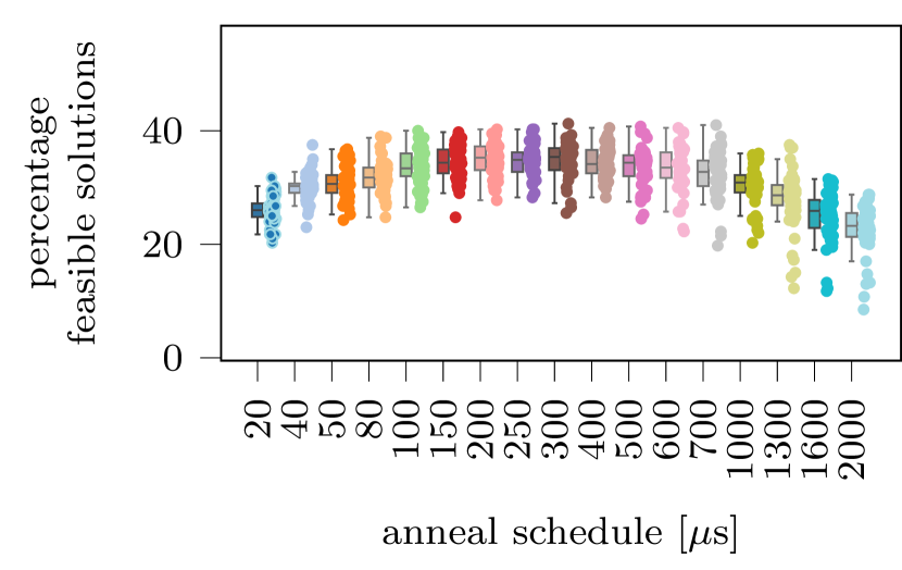
(a) s-trp_6.

(b) s-trp_7.

(c) s-trp_8.

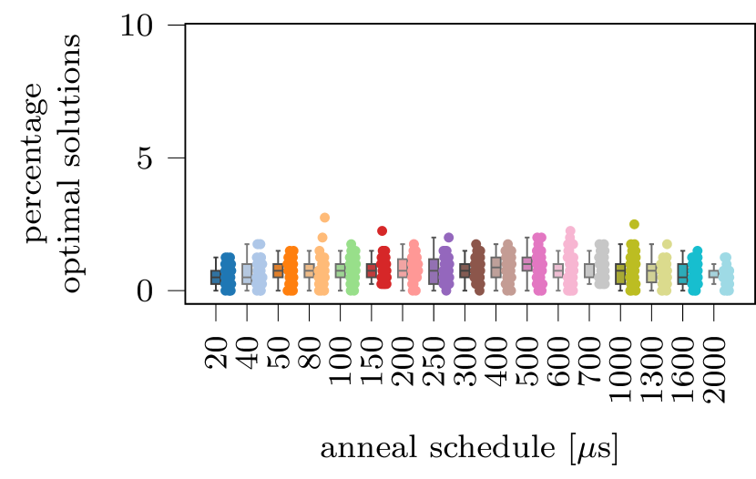
(d) s-trp_6.

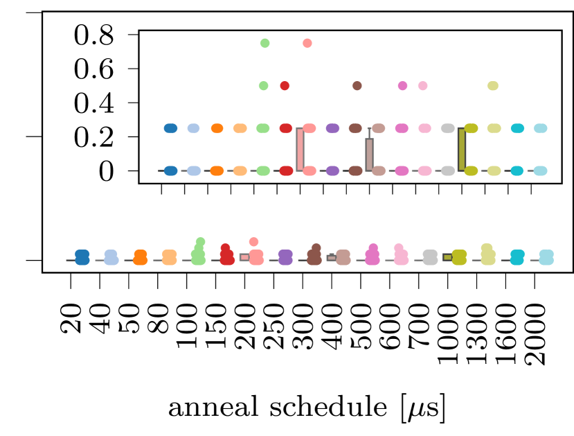
(e) s-trp_7.

(f) s-trp_8.

Figure 45: Percentage of feasible and optimal solutions for symmetrical distribution of cities with different anneal schedules. The chain strength values of $0.6$ is used for s-trp_6 and $0.9$ for s-trp_7, and s-trp_8. The number of anneal reads are 20000 for each anneal schedule. Clique embedding was used to embed the QUBO. The calculations were executed on Advantage 4.1 and results were obtained on 2023/11/24.

6 Conclusion

Quantum computers have undergone an impressive development in recent decades as it can be observed, for example, by the continuously increasing qubit numbers, the decreasing error rates, or from a plurality of component or system level benchmarks. This advancement has sparked interest in a large variety of domains and the promise of solving the most challenging computational problems in each discipline is in the air. Both, the current quantum computing systems as well as the quantum software stack, are now mature enough to review this promise. It is critical to accomplish this not only on an academic level but more importantly for industry relevant applications.

In this spirit, we considered in this paper two industry use cases from the field of discrete optimization, which is among the most prominent candidates for the application of quantum computing. We carried out extensive and systematic experiments on the superconducting IBM quantum computers as well as on a D-Wave quantum annealer to illustrate the current status of these technologies for optimization problems. Our main conclusion is that there are still significant challenges on the way to a practical use. In particular, we observe that on the IBM quantum systems only small proof-of-concept examples can be executed with an acceptable quality. For larger problem instances the solution quality quickly deteriorates and throughout all examples we find a lack of reproducibility and predictability. However, comparing the different generations of IBM quantum processors we could clearly observe the improvement of the result quality with the evolution of the hardware. On the more mature quantum annealing system of D-Wave we could execute larger problem instances bringing us one step closer from proof-of-concept to real-world examples. Nevertheless, again the solution quality decreases with the problem size which poses a clear limit to the usability also of quantum annealers for industry relevant problems.

In summary, this paper gave a comprehensive insight into the current state of quantum computing based on two industry relevant optimization problems. While we observed that today’s quantum computers are still limited, the examples and experiments in this paper provide a blueprint to track the progress and the readiness for real world applications of the fast evolving quantum computing ecosystem.

Code Availability

The implementation of the LamA use case and of the corresponding example series can be found here. The truck routing use case is available here. The IBM and D-Wave experiment data is available on request.

Appendix A Additional Results for LamA Use Case

In this part of the appendix, we provide the convergence plots of the classical optimizer COBYLA for lama_0p2 and lama_2p3. The setup is the same as described in detail in Section 4.1 and in Figure 7 for lama_1p3.

Appendix B Information on IBM Quantum Computing Resources

In this part of the appendix, we provide background information on the IBM quantum computing systems, on which we the experiments presented in this paper were executed. The data stems from the dates when these experiments where carried out.

References

- [1] D.-S. Chen, R. G. Batson, and Y. Dang. “Applied integer programming: Modeling and solution”. Wiley. Hoboken, NJ (2010).
- [2] A. Schrijver. “Theory of linear and integer programming”. A Wiley-Interscience publication. Wiley. Chichester and Weinheim (2000). Reprinted edition. url: https://www.wiley.com/en-us/Theory+of+Linear+and+Integer+Programming-p-9780471982326.
- [3] A. Bayerstadler, G. Becquin, J. Binder, T. Botter, H. Ehm, T. Ehmer, M. Erdmann, N. Gaus, P. Harbach, M. Hess, J. Klepsch, M. Leib, S. Luber, A. Luckow, M. Mansky, W. Mauerer, F. Neukart, C. Niedermeier, L. Palackal, R. Pfeiffer, C. Polenz, J. Sepulveda, T. Sievers, B. Standen, M. Streif, T. Strohm, C. Utschig-Utschig, D. Volz, H. Weiss, and F. Winter. “Industry quantum computing applications”. EPJ Quantum Technology 8, 1–17 (2021).
- [4] A. Luckow, J. Klepsch, and J. Pichlmeier. “Quantum computing: Towards industry reference problems”. Digitale Welt 5, 38–45 (2021).
- [5] S. Yarkoni, E. Raponi, T. Bäck, and S. Schmitt. “Quantum annealing for industry applications: Introduction and review”. Reports on progress in physics. Physical Society (Great Britain) 85, 104001 (2022).
- [6] E. Farhi, J. Goldstone, and S. Gutmann. “A quantum approximate optimization algorithm” (2014). arXiv:1411.4028.
- [7] A. Peruzzo, J. McClean, P. Shadbolt, M.-H. Yung, X.-Q. Zhou, P. J. Love, A. Aspuru-Guzik, and J. L. O’Brien. “A variational eigenvalue solver on a photonic quantum processor”. Nature Communications 5, 4213 (2014).
- [8] A. Abbas, A. Ambainis, B. Augustino, A. Baertschi, H. Buhrman, C. Coffrin, G. Cortiana, V. Dunjko, D. Egger, B. Elmegreen, N. Franco, F. Fratini, B. Fuller, J. Gacon, C. Gonciulea, S. Gribling, S. Gupta, S. Hadfield, R. Heese, G. Kircher, T. Kleinert, T. Koch, G. Korpas, S. Lenk, J. Marecek, V. Markov, G. Mazzola, S. Mensa, N. Mohseni, G. Nannicini, C. O’Meara, E. Peña Tapia, S. Pokutta, M. Proissl, P. Rebentrost, E. Sahin, B. Symons, S. Tornow, V. Valls, S. Woerner, M. Wolf-Bauwens, J. Yard, S. Yarkoni, D. Zechiel, S. Zhuk, and C. Zoufal. “Quantum optimization: Potential, challenges, and the path forward” (2023). arXiv:2312.02279.
- [9] E. Knill, D. Leibfried, R. Reichle, J. Britton, R. B. Blakestad, J. D. Jost, C. Langer, R. Ozeri, S. Seidelin, and D. J. Wineland. “Randomized benchmarking of quantum gates”. Physical review. A, Atomic, molecular, and optical physics 77, 012307 (2008).
- [10] E. Magesan, J. M. Gambetta, and J. Emerson. “Scalable and robust randomized benchmarking of quantum processes”. Physical review letters 106, 180504 (2011).
- [11] E. Nielsen, J. K. Gamble, K. Rudinger, T. Scholten, K. Young, and R. Blume-Kohout. “Gate set tomography”. Quantum 5, 557 (2021).
- [12] A. W. Cross, L. S. Bishop, S. Sheldon, P. D. Nation, and J. M. Gambetta. “Validating quantum computers using randomized model circuits”. Physical Review A 100, 032328 (2019).
- [13] J. Nelson, M. Vuffray, A. Y. Lokhov, and C. Coffrin. “Single-qubit fidelity assessment of quantum annealing hardware” (2021). arXiv:2104.03335.
- [14] T. Zaborniak and R. de Sousa. “Benchmarking Hamiltonian noise in the D-Wave quantum annealer”. IEEE Transactions on Quantum Engineering 2, 1–6 (2021).
- [15] J. R. Finzgar, P. Ross, L. Holscher, J. Klepsch, and A. Luckow. “Quark: A framework for quantum computing application benchmarking”. In 2022 IEEE International Conference on Quantum Computing and Engineering. Pages 226–237. IEEE (2022).
- [16] T. Lubinski, S. Johri, P. Varosy, J. Coleman, L. Zhao, J. Necaise, C. H. Baldwin, K. Mayer, and T. Proctor. “Application-oriented performance benchmarks for quantum computing”. IEEE Transactions on Quantum Engineering 4, 1–32 (2023).
- [17] T. Lubinski, C. Coffrin, C. McGeoch, P. Sathe, J. Apanavicius, and D. E Bernal Neira. “Optimization applications as quantum performance benchmarks” (2024). arXiv:2302.02278.
- [18] T. Tomesh, P. Gokhale, V. Omole, G. S. Ravi, K. N. Smith, J. Viszlai, X.-C. Wu, N. Hardavellas, M. R. Martonosi, and F. T. Chong. “Supermarq: A scalable quantum benchmark suite”. In 2022 IEEE International Symposium on High-Performance Computer Architecture. Pages 587–603. Piscataway, NJ (2022). IEEE.
- [19] S. Karimi and P. Ronagh. “Practical integer-to-binary mapping for quantum annealers”. Quantum Information Processing 18, 1–24 (2019).
- [20] M. A. Nielsen and I. L. Chuang. “Quantum computation and quantum information”. Cambridge University Press. Cambridge (2010). 10th anniversary edition.
- [21] A. Sturm. “Theory and implementation of the quantum approximate optimization algorithm: A comprehensible introduction and case study using qiskit and ibm quantum computers” (2023). arXiv:2301.09535.
- [22] M. Cerezo, A. Arrasmith, R. Babbush, S. C. Benjamin, S. Endo, K. Fujii, J. R. McClean, K. Mitarai, X. Yuan, L. Cincio, and P. J. Coles. “Variational quantum algorithms”. Nature Reviews PhysicsPages 1–20 (2021).
- [23] T. Kadowaki and H. Nishimori. “Quantum annealing in the transverse ising model”. Physical Review E 58, 5355–5363 (1998).
- [24] S. Kirkpatrick, C. D. Gelatt, and M. P. Vecchi. “Optimization by simulated annealing”. Science (New York, N.Y.) 220, 671–680 (1983).
- [25] G. E. Santoro, R. Martonák, E. Tosatti, and R. Car. “Theory of quantum annealing of an Ising spin glass”. Science (New York, N.Y.) 295, 2427–2430 (2002).
- [26] R. Martonák, G. E. Santoro, and E. Tosatti. “Quantum annealing of the traveling-salesman problem”. Physical review. E, Statistical, nonlinear, and soft matter physics 70, 057701 (2004).
- [27] V. S. Denchev, S. Boixo, S. V. Isakov, N. Ding, R. Babbush, V. Smelyanskiy, J. Martinis, and H. Neven. “What is the computational value of finite-range tunneling?”. Physical Review X6 (2016).
- [28] D. A. Battaglia, G. E. Santoro, and E. Tosatti. “Optimization by quantum annealing: Lessons from hard satisfiability problems”. Physical review. E, Statistical, nonlinear, and soft matter physics 71, 066707 (2005).
- [29] E. Boyda, S. Basu, S. Ganguly, A. Michaelis, S. Mukhopadhyay, and R. R. Nemani. “Deploying a quantum annealing processor to detect tree cover in aerial imagery of california”. PloS one 12, e0172505 (2017).
- [30] F. Neukart, G. Compostella, C. Seidel, D. von Dollen, S. Yarkoni, and B. Parney. “Traffic flow optimization using a quantum annealer”. Frontiers in ICT 4, 301656 (2017).
- [31] D. O’Malley, V. V. Vesselinov, B. S. Alexandrov, and L. B. Alexandrov. “Nonnegative/binary matrix factorization with a D-Wave quantum annealer”. PloS one 13, e0206653 (2018).
- [32] C. C. McGeoch. “Adiabatic quantum computation and quantum annealing”. Springer International Publishing. Cham (2014).
- [33] T. Albash and D. A. Lidar. “Adiabatic quantum computing”. Reviews of Modern Physics 90, 833 (2018).
- [34] M. Born and V. Fock. “Beweis des Adiabatensatzes”. The European Physical Journal A 51, 165–180 (1928).
- [35] B. Heim, T. F. Rønnow, S. V. Isakov, and M. Troyer. “Quantum versus classical annealing of Ising spin glasses”. Science 348, 215–217 (2015).
- [36] R. Martonák, G. E. Santoro, and E. Tosatti. “Quantum annealing of the traveling-salesman problem”. Physical review. E, Statistical, nonlinear, and soft matter physics 70, 057701 (2004).
- [37] C. Baldassi and R. Zecchina. “Efficiency of quantum vs. classical annealing in nonconvex learning problems”. Proceedings of the National Academy of Sciences 115, 1457–1462 (2018).
- [38] IBM. “Processor types”. url: https://docs.quantum.ibm.com/run/processor-types. (accessed: 06.03.2024).
- [39] IBM. “Compute resources”. url: https://quantum.ibm.com/services/resources. (accessed: 06.03.2024).
- [40] IBM. “ECR gate”. url: https://docs.quantum.ibm.com/api/qiskit/qiskit.circuit.library.ECRGate. (accessed: 06.03.2024).
- [41] V. Choi. “Minor-embedding in adiabatic quantum computation: I. The parameter setting problem”. Quantum Information Processing 7, 193–209 (2008).
- [42] D-Wave. “D-Wave QPU architecture: Topologies”. url: https://docs.dwavesys.com/docs/latest/c_gs_4.html. (accessed: 06.03.2024).
- [43] E. Grant and T. S. Humble. “Benchmarking embedded chain breaking in quantum annealing”. Quantum Science and Technology 7, 025029 (2022).
- [44] S. Okada, M. Ohzeki, M. Terabe, and S. Taguchi. “Improving solutions by embedding larger subproblems in a d-wave quantum annealer”. Scientific Reports 9, 2098 (2019).
- [45] D-Wave. “Ocean software documentation - minor-embedding”. url: https://docs.ocean.dwavesys.com/en/stable/concepts/embedding.html. (accessed: 06.03.2024).
- [46] D-Wave. “System documentation - programming the D-Wave QPU: Setting the chain strength”. url: https://www.dwavesys.com/media/vsufwv1d/14-1041a-a_setting_the_chain_strength.pdf. (accessed: 06.03.2024).
- [47] D-Wave. “System documentation - solver parameters”. url: https://docs.dwavesys.com/docs/latest/c_solver_parameters.html. (accessed: 06.03.2024).
- [48] O. Galindo and V. Kreinovich. “What is the optimal annealing schedule in quantum annealing”. In 2020 IEEE Symposium Series on Computational Intelligence (SSCI). Pages 963–967. IEEE (2020).
- [49] C. Carugno, M. Ferrari Dacrema, and P. Cremonesi. “Evaluating the job shop scheduling problem on a D-Wave quantum annealer”. Scientific Reports 12, 6539 (2022).
- [50] E. Pelofske, G. Hahn, and H. Djidjev. “Advanced anneal paths for improved quantum annealing”. Proceedings - IEEE International Conference on Quantum Computing and Engineering, QCE 2020Pages 256–266 (2020).
- [51] Fraunhofer IAO. “LamA - Laden am Arbeitsplatz”. url: https://www.lama.zone/. (accessed: 06.03.2024).
- [52] N. Ezzell, B. Pokharel, L. Tewala, G. Quiroz, and D. A. Lidar. “Dynamical decoupling for superconducting qubits: A performance survey”. Physical Review Applied 20, 064027 (2023).
- [53] Y. Kim, C. J. Wood, T. J. Yoder, S. T. Merkel, J. M. Gambetta, K. Temme, and A. Kandala. “Scalable error mitigation for noisy quantum circuits produces competitive expectation values”. Nature Physics 19, 752–759 (2023).
- [54] P. D. Nation and M. Treinish. “Suppressing quantum circuit errors due to system variability”. PRX Quantum 4, 010327 (2023).
- [55] A. Ketterer and T. Wellens. “Characterizing crosstalk of superconducting transmon processors”. Phys. Rev. Appl. 20, 034065 (2023).
- [56] E. Pelofske. “4-clique network minor embedding for quantum annealers”. LA-UR-23- (2024). url: http://arxiv.org/pdf/2301.08807.pdf.
- [57] D-Wave. “System documentation - reformulating a problem”. url: https://docs.dwavesys.com/docs/latest/handbook_reformulating.html. (accessed: 06.03.2024).