Crossing walls and windows: the curious escape of Lyman-$\alpha$ photons through ionised channels

Abstract

The diverse Lyman-alpha ( Ly$\alpha$) line profiles are essential probes of gas in and around galaxies. While isotropic models can successfully reproduce a range of  Ly$\alpha$ observables, the correspondence between the model and actual physical parameters remains uncertain. We investigate the effect of anisotropies of Ly$\alpha$ escape using a simplified setup: a hole (fractional size $\tilde{s}$) within a semi-infinite slab with constant column density. Due to the slab’s high line-centre optical depth ($\tau_{0}\gtrsim 10^{5-6}$), most photons should escape through the empty channel. However, our numerical findings indicate that only a fraction $\sim\tilde{s}$ of photons exit through this channel. To explain this puzzle, we developed an analytical model describing the scattering and transmission behaviour of  Ly$\alpha$ photons in an externally illuminated slab. Our findings show that the number of scatterings per reflection follows a Lévy distribution ($\propto N^{-3/2}$). This means that the mean number of scatterings is orders of magnitude greater than expectations, facilitating a shift in frequency and the subsequent photon escape. Our results imply that  Ly$\alpha$ photons are more prone to traverse high-density gas and are surprisingly less biased to the ‘path of least resistance’. Hence,  Ly$\alpha$ can trace an averaged hydrogen distribution rather than only low-column density ‘channels’.

1 Introduction

The Universe’s brightest spectral line, Lyman-$\alpha$ ( Ly$\alpha$) plays a critical role in various fields of astronomy and astrophysics. Since the  Ly$\alpha$ line profile is sensitive to the gas column density  (Adams, 1972; Neufeld, 1990; Dijkstra et al., 2006), gas kinematics  (Bonilha et al., 1979; Ahn & Lee, 2002), dust  (Neufeld, 1990; Laursen et al., 2009) and fragmentation (Neufeld, 1991; Hansen & Oh, 2006; Gronke et al., 2016), it provides crucial information about the gas that photons traverse on their journey to the observer. Hence,  Ly$\alpha$ has been an effective tool for studying the properties of the interstellar medium (ISM), the circumgalactic medium (CGM), and its spatial distribution  (e.g., Steidel et al., 2010; Wisotzki et al., 2016) as well as for exploring galaxies with the highest redshifts  (Dijkstra, 2014; Barnes et al., 2014; Ouchi et al., 2020).

As  Ly$\alpha$ is a resonant line undergoing complex radiative transfer effects, decoding the information imprinted in the line profile remains a complex and unsolved challenge. Most attempts so far have relied on isotropic models that succeed at reproducing the line profile using simple geometries  (e.g., Verhamme et al., 2006; Dijkstra et al., 2006). However, these models still leave unclear how the fitted parameters relate to actual physical conditions (e.g.,  Orlitová et al. 2018; Gronke & Dijkstra 2016; Li & Gronke 2022). Factually, astrophysical gas configurations are highly anisotropic. Such anisotropies play an influential role in shaping the  Ly$\alpha$ profile. This is confirmed by studies of  Ly$\alpha$ radiative transfer through varied geometries in simplified  (e.g., Behrens & Braun, 2014; Zheng & Wallace, 2014; Chang et al., 2024) and more complex  (e.g. Smith et al., 2022; Kim et al., 2023) setups. A notable fitted parameter is the neutral gas column density ($N_{\rm HI}$). Given the multi-phase and anisotropic nature of the gas, we anticipate realistic column densities to be distributed within a wide range of values. However, current models yield only one value of $N_{\rm HI}$, leaving unresolved whether this quantity represents the mean of the distribution or is skewed towards lower densities where photons are more easily transmitted.

Accounting for anisotropies is essential for understanding the ISM. Stellar feedback, for instance, significantly contributes to this anisotropy by generating channels filled with a hot gas phase  (Cox & Smith, 1974; McKee & Ostriker, 1977). These low-density channels should also be imprinted in the  Ly$\alpha$ line and offer a prime opportunity for radiation to escape and reach the observer  (Zackrisson et al., 2013). It is commonly asserted that within a porous ISM  Ly$\alpha$ primarily probes the gas phases with the lowest column density, essentially tracing the ‘path of the least resistance’  (Jaskot et al., 2019; Kakiichi & Gronke, 2021). However, the extent to which other phases in the distribution contribute remains uncertain.

These low $N_{\rm HI}$ channels are of particular importance as their presence might be crucial to allow ionising photons to escape their host galaxy and to re-ionise the Universe (Zackrisson et al., 2013; Rivera-Thorsen et al., 2017; Herenz et al., 2017; Bik et al., 2018). Since  Ly$\alpha$ and Lyman Continuum (LyC) probe the same neutral hydrogen,  Ly$\alpha$ is a valuable tool for inferring ionising escape fractions and understanding LyC escape (Verhamme et al., 2015; Dijkstra et al., 2016; Izotov et al., 2018). However, thus far it is unclear how this proxy for LyC escape is influenced by an anisotropic gas distribution, that is, whether  Ly$\alpha$ correlates with a ‘line-of-sight’ LyC escape fraction or a ‘global one’ – important for models of the epoch of ionisation.

Given this inherently anisotropic nature of realistic neutral hydrogen distributions in and around galaxies, there is a growing need for a model that accounts for diverse gas distributions. Furthermore, no firm theoretical understanding of anisotropic  Ly$\alpha$ escape has been established. In this letter, we first introduce the problem of anisotropic  Ly$\alpha$ escape on a simplified, theoretical basis (§ 2). Then, we test our theoretical model in § 3 using results of Monte Carlo radiative transfer (RT) simulations before we discuss these results within a broader framework in § 4. We discuss and conclude in § 5.

2 Analytical considerations

2.1 Setup and first estimate

In order to understand the escape of  Ly$\alpha$ through an anisotropic medium let us consider the simple case of a static, semi-infinite slab with column density $N_{{\text{H{I}}}}$ and temperature $T$ in which an empty hole is carved on one side with a surface area fraction $\tilde{s}$.This setup can be seen as a simplification of the complex distribution of hydrogen column densities of a porous ISM, as described above. All the  Ly$\alpha$ photons are emitted near the line centre in the midplane, where a cavity allows the initial diffusion to escape from the hole. Fig. 1 shows a sketch of the considered setup.

The question we want to answer is which fraction of the flux will escape through the hole and which fraction will escape through the slab, that is, $\tilde{f}=F_{\rm hole}/F_{\rm slab}$. To first order, we can infer that the photons escaping through the slab form a broad double-peaked spectrum (Adams, 1972; Neufeld, 1990), and those escaping through the hole exiting with a frequency near the line centre. Thus, $\tilde{f}$ will set the emergent  Ly$\alpha$ spectrum (cf. illustration in Fig. 1). Using radiative transfer simulations, we confirm in § 4 that this picture is not far from the truth.

A very naive first estimate would be that $F_{\rm hole}\propto\tilde{s}$ and $F_{\rm slab}\propto\exp(-\tau_{\rm i})$ where $\tau_{\rm i}=N_{\text{H{I}}}\sigma(x=x_{i})$ is the optical depth at the emitted frequency $x_{\rm i}=(\nu-\nu_{0})/\Delta\nu$, expressed here in Doppler shifts from line centre frequency $\nu_{0}$ (with $\Delta\nu=c(\nu/\nu_{0}-1)/v_{\rm th}$ and $v_{\rm th}$ is the thermal velocity). This estimate would yield, with $\tilde{s}\sim 0.1$ and $N_{\text{H{I}}}=10^{19}\,{{\mathrm{cm}}}^{-2}$, that essentially all the photons would escape through the hole, i.e., $\tilde{f}\rightarrow\infty$, since $\tau(x=x_{\rm i}=0)\approx 6\times 10^{5}$ at $T=10^{4}\,$K. This approximation is clearly an oversimplification since the $\exp(-\tau_{\rm i})$ term does not include the resonant nature of  Ly$\alpha$. However, it illustrates the basic property of this setup, namely that for  Ly$\alpha$ photons, it is significantly easier to escape through the hole than through the slab.

Neufeld (1990) analytically solved the  Ly$\alpha$ radiative transfer equation for a static, homogeneous slab, yielding a functional expression for the emergent spectrum alongside several additional properties. He found, for instance, that the transmission probability of incoming radiation is $T_{\rm slab}=4/(3\tau_{\rm i})$. Thus, it would take $N_{\rm sc}^{\rm slab}=1/T_{\rm slab}\sim\tau_{\rm i}$ scatterings to escape through the slab. During these scatterings, the  Ly$\alpha$ photons can bounce off the walls of the cavity, and for each reflection, they have a probability of $\tilde{s}$ to escape through the hole. Hence, this improved estimate would yield $\tilde{f}\sim\tilde{s}/T_{\rm slab}\sim\tilde{s}\tau_{\rm i}$ which for the above-used values would equal $\sim 10^{4}$. Still, nearly all the flux should pass through the hole, forming a centrally peaked spectrum.

This picture leaves several problems. Firstly, this seems to be contradicting observations. Although the ISM is porous (McKee & Ostriker, 1977), we do not observe many centrally peaked  Ly$\alpha$ spectra as most are double-peaked or have a redshifted single peak (e.g., Erb et al., 2014; Yang et al., 2016; Hayes et al., 2021). In addition, for the few objects in which a triple peak is present (Dahle et al., 2016; Rivera-Thorsen et al., 2017, 2019; Vanzella et al., 2020), the flux ratio of the outer to the inner peaks is $\mathcal{O}(1)$ but the peak separation of the outer peaks indicates column densities of $\sim 10^{19}\,{{\mathrm{cm}}}^{-2}$ (cf. Rivera-Thorsen et al., 2017), implying a very small, highly fine-tuned $\tilde{s}$. The major problem with the above picture, however, is also that radiative transfer simulations of anisotropic  Ly$\alpha$ escape as the ones we will present in § 4 indicate much smaller central peak fluxes around $\tilde{f}\sim\mathcal{O}(1)$ (see also numerical results by Behrens & Braun, 2014, who performed a range of  Ly$\alpha$ radiative transfer simulations through anisotropic, outflowing media).

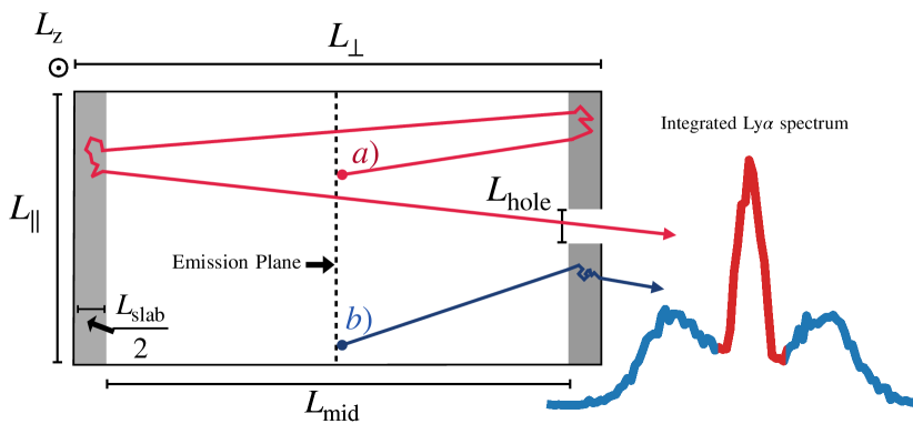
Figure 1: Simulation setup to investigate the impact of non-homogeneous gas distributions on the  Ly$\alpha$ profile. Anisotropy is introduced by incorporating a square hole with a side length of $L_{\rm hole}$ along the non-periodic direction (see § 3 for more information). The arrow marked as a) shows the path followed by an example photon that was reflected and bounced inside the slab before encountering the hole. Arrow b) illustrates the path of a photon directly transmitted through the slab. The colour coding of the  Ly$\alpha$ line shown on the right indicates the origin of the spectrum components

Figure 2:  Ly$\alpha$ spectra obtained from gas-filled slabs with an empty hole at varying $N_{\rm HI}$. The $\tilde{s}=0$ case corresponds to a homogeneous slab without a hole (marked in the lightest colour). The rest of the curves represent spectra with empty channels of different sizes. The dimensionless photon frequency is displayed on the x-axis.

2.2 A novel picture of  Ly$\alpha$ photon escape

The problem with the above is that we assumed the  Ly$\alpha$ photons ‘bounce’ off the optically thick wall of the slab as if they were ping-pong balls. Thus, since every (other) reflection offers the photon a chance to escape through the hole but every scatter offers a chance to shift so much in frequency that the photon escapes through the slab, setting the number of scatters equal to the number of reflections is wrong. While it is tempting to assume that due to the difficulty in penetrating the slab, the photons scatter only a few times per reflection, let us first compute this number analytically. This problem is analogous to the ‘Gambler’s ruin’ problem. In this, a gambler starts with an initial sum of $w_{0}=\$1$ and has a $p=1/2$ probability of winning/losing $\$1$; similar to the  Ly$\alpha$ photon that enters the slab a depth $\sim\lambda_{\rm mfp}=(\sigma n_{\text{H{I}}})^{-1}$ and will move forward / backwards $\sim\lambda_{\rm mfp}$ (ignoring frequency redistribution).

To estimate the mean number of scatterings per reflection (or the mean number of games before ruin), we can solve the usual diffusion equation $\partial_{t}p=\sigma^{2}\partial^{2}_{z}p/2$ with $p(0,z)=\delta(z-z_{0})$ as initial condition and $\sigma^{2}=\lambda_{\rm mfp}c$, and time $t$ or number of scatterings $N_{\rm scatter}=tc/\lambda_{\rm mfp}$ used interchangeably.

If we consider the edge of the slab as an absorbing barrier located at $z_{\rm b}=0$, we have the additional constraint $p(t,z=0)=0$. This boundary value problem can be solved using the initial conditions $p(0,z)=\delta(z-z_{0})-A\delta(z-B)$ for which $A$ and $B$ are chosen so that the two evolving peaks cancel each other exactly at $z=z_{\rm b}$, i.e., $p(t,z_{\rm b})=0$ is fulfilled. The solution of the diffusion equation with these initial conditions is due to the linearity of the problem, simply two widening Gaussians with variance $\sigma^{2}t$ and means $\pm z_{0}$. To obtain the mean number of scatterings per reflection, let’s consider the cumulative fraction of photons that have been reflected at time $t$:

$$F_{\rm reflected}(t)=1-\int\limits_{0}^{\infty}p(t,z)\mathrm{d}z=1-\mathrm{erf}\left(\frac{z_{0}}{\sqrt{2t}\sigma}\right)$$ (1)

where $\mathrm{erf}$ is the error function. Thus, the ones that are reflected within $[t\pm{\rm d}t/2]$ are given by

$$f_{\rm reflected}(t)=\frac{\mathrm{d}F_{\rm reflected}}{\mathrm{d}t}= \frac{z_{0}}{\sqrt{2\pi t^{3}\sigma^{2}}}\exp\left(-\frac{(z_{0})^{2}}{2t\sigma^{2}}\right)$$ (2)

$$\text{or }f_{\rm reflected}(N_{\rm scatter})= \frac{1}{\sqrt{2\pi N_{\rm scatter}^{3}}}\exp\left(-\frac{1}{2N_{\rm scatter}}\right)$$ (3)

which is a Levy distribution with scale $c_{\rm L}=1$ and location $\mu_{\rm L}=0$. Note that for large number of scatterings, we obtain $f_{\rm reflected}\propto N_{\rm scatter}^{-3/2}$.

Thus, the mean number of scatterings per reflection is simply

$$\bar{N}_{\rm scatter}=\int\limits_{0}^{\tau_{0}}nf_{\rm reflected}(n)\mathrm{d}n=\sqrt{\frac{2\tau_{0}}{\pi}}.$$ (4)

The above equations are the more general case of the ‘Gambler’s ruin’ problem described above. Eq. (1) shows that eventually all gamblers are ruined ($F_{\rm reflected}\rightarrow 1$ as $t\rightarrow\infty$) but on average they stay infinitely long in the casino ($\bar{N}_{\rm scatter}\rightarrow\infty$ for $\tau_{0}\rightarrow\infty$; cf. Eq. (4)). However,  Ly$\alpha$ photons are saved from this destiny due to their eventual shift in frequency to $x\gtrsim x_{\rm esc}$, where $x_{\rm esc}$ is a frequency that allows for escape (Adams, 1972; Neufeld, 1990).

An additional result one can obtain from the above considerations is that the transmission probability through a slab is given by

$$T_{\rm slab}= \alpha\int_{\tau_{0}}^{\infty}f_{\rm reflected}(n)\mathrm{d}n\approx(2\pi\tau_{0})^{-1/2}$$ (5)

where we have used that on average $\tau_{0}$ are required in order to shift to an escape frequency (Adams, 1972). The additional factor of $\alpha$ arises because even once $x\gtrsim x_{\rm esc}$, the photon can escape forward through the slab or return backwards. Thus, if $\tau(x_{\rm esc})\lesssim 1$, these final escape paths are equally likely and $\alpha=1/2$. However, for very large optical depths the photon will undergo a second ‘Gamblers ruin’ problem with $x\approx x_{\rm esc}$ with, however, the chance to ‘win sufficient money to leave’, i.e., reach the far end. In that case, $\alpha\approx 4/(3\tau(x_{\rm esc}))$ following the original Neufeld (1990) argument. Since this regime only applies for $a_{\rm v}\tau_{0}>1000$, i.e., very low temperatures or high optical depths, we will explore this regime in future work and here simply use $\alpha=1/2$ (as in the last step in Eq. (5)).

With these results at hand, we can now estimate the fraction of photons escaping through the hole as

$$\tilde{f}\approx\frac{N_{\rm scatter}^{\rm slab}/\bar{N}_{\rm scatter}}{N_{\rm refl}^{\rm hole}}\approx\frac{\tilde{s}/2}{T_{\rm slab}\bar{N}_{\rm scatter}}=\frac{\pi}{2}\tilde{s}$$ (6)

where $N_{\rm refl}^{\rm hole}\simeq 2/\tilde{s}$ is the number of reflections needed to escape through the hole. Eq. (6) shows two interesting things: (i) a simple $\tilde{f}\sim\tilde{s}$ behaviour leading to a relatively low escape fraction through the hole (more in line with the observations discussed above), and (ii) no dependence on $\tau_{0}$ which seems counter-intuitive as one might think of  Ly$\alpha$ escaping preferentially through low column density channels. We will compare these analytical estimates to our numerical findings in § 4.

3 Numerical Method

To test the theory presented in the previous section, we conducted  Ly$\alpha$ radiative transfer simulations using the Monte Carlo radiative transfer code tlac (Gronke & Dijkstra, 2014) which follows  Ly$\alpha$ photon packages in real and frequency space taking into account scattering with HI (see, e.g., Dijkstra, 2014, for an explanation of the technique). These simulations were conducted on a semi-infinite slab of size $L_{\parallel}\times L_{\perp}\times L_{\rm z}$ where the sides $L_{\parallel}$ and $L_{z}$ are periodic and $L_{\parallel}=L_{\rm z}$. The slab contains static neutral hydrogen with fixed column density (from the emission plane to the boundary) $N_{\rm HI}\in[10^{17},10^{21}]\ \,{{\mathrm{cm}}}^{-2}$. Using these parameters, we generated two different groups of simulations:

1. Semi-infinite slab with an empty hole. The first group is to investigate the impact of non-homogeneous gas distributions on the  Ly$\alpha$ profile by introducing anisotropies into the setup. Specifically, we aim to compare the theory developed in § 2 to radiative transfer simulations. We placed the emission plane at the midpoint relative to the finite direction (i.e. at $L_{\perp}/2$) and set up the grid such that $L_{\perp}=L_{\rm mid}+L_{\rm slab}$ with an empty region of width $L_{\rm mid}$ and two thin HI layers of total width $L_{\rm slab}$ located at the extremes. To introduce an anisotropy, we carve a square hole orthogonal to the emission plane with a side length $L_{\rm hole}$, as illustrated by Fig. 1. This results in an opening area of $\tilde{s}\equiv L_{\rm hole}^{2}/(L_{\parallel}L{\rm z})$. In this set of simulations, we maintained the gas temperature at $T=10^{4}$ K. In the derivation of § 2, the slab is assumed to be infinitely thin, and the probability of hitting the hole is independent of the reflecting position on the far side of the setup. These conditions are fulfilled if $L_{\rm slab}\ll L_{\rm hole}$ and $L_{\rm mid}\gg L_{\parallel}$, respectively. We thus chose $L_{\perp}=50\ L_{\parallel}$ and $L_{\rm slab}=2\times 10^{-3}\ L_{\perp}$. For this study, we validated that changes in these parameters, within a factor of a few, do not affect our results. We will expand to a spherical setup and explore other effects of geometry in a follow-up paper. .

2. Externally illuminated slab. The second group of simulations is to test how many scatterings occur per reflection. We created a slab externally illuminated from one side by positioning the photon emission plane at the bottom of the slab. Here, photons either traverse the slab entirely to the opposite side and are transmitted or penetrate the slab and scatter freely before being reflected. We conducted these at three different temperatures $T=10^{2}$, $10^{4}$ and $10^{6}$ K.

We generally used $10^{3}$- $10^{6}$ photon packages to obtain a converged result and used $100\times 5000\times 100$ cells in order to resolve the hole as well as the HI layer.

Figure 3: Distribution of the scattering number for an externally illuminated slab. The shades of blue indicate different values of optical depth. The red curve shows the analytical form derived from Eq. 3.

4 Numerical Results

4.1  Ly$\alpha$ spectra of a slab with a hole

Fig. 2 shows the emergent  Ly$\alpha$ spectra obtained from radiative transfer simulations as described in § 31, at three different column density values. Each panel presents spectra from slabs with carved holes of various sizes $\tilde{s}$, including a homogeneous slab ($\tilde{s}=0$). At first glance, spectra from the homogeneous slab show the expected blue- and red-shifted peaks resulting from frequency diffusion. In contrast, spectra from a slab with a carved hole show flux near the line centre on top of the expected blue and red peaks.

Take, for instance the last panel in Fig. 2 with $N_{\rm HI}=10^{20}\ \rm cm^{-2}$ and $\tau_{0}\sim 6\times 10^{5}$. According to the discussion in § 2.1, for all values of $\tilde{s}$ in this figure, the fraction $\tilde{f}\simeq\tilde{s}\tau_{0}$ indicates a central flux at least four orders of magnitude greater than the one escaping from the slab. In other words, most photons should exit through the hole, resulting in a single-peaked $\,{{\mathrm{Ly}\alpha}}$ line profile near the line centre. Evidently, the spectra in Fig. 2 contradict this prediction, as they show central fluxes with roughly the same order of magnitude as the red and blue peaks. We will further explore this central peak inconsistency in § 4.3.

4.2 Transmission and scattering statistics of an externally illuminated slab

The alternative theory outlined in § 2.2 proposes that  Ly$\alpha$ photons undergo a large number of scatterings before being reflected by the slab. To test this hypothesis, we examined the scattering behaviour of photons in a slab with an externally illuminated slab as described in § 32. In such a setting, photons can be either transmitted to the other side or reflected by the slab. Due to the medium’s high optical depth, the majority of the photons get reflected upon encountering the slab. These reflected photons do not simply bounce/reflect as in a mirror but penetrate a small portion of the slab instead and ‘random walk’ their way out. Consequently, the number of scatterings per reflection ($N_{\rm scatter}$) is significantly larger than the ‘simple reflection’ scenario (where $N_{\rm scatter}=1$).

Fig. 3 displays the distribution of the number of scatterings per reflection $N_{\rm scatter}$ for photons reflected by slabs with three selected line centre optical depths at $T=10^{4}$ K. As anticipated by Eq. 3, this approximates a Levy distribution, which for large values of $N_{\rm scatter}$, simplifies to a power law with an exponent of $-3/2$ (marked with a red line in Fig. 3). Accordingly, photons are expected to undergo an average $\bar{N}_{\rm scatter}\propto\sqrt{\tau_{0}}\$ scatterings (as given by Eq. 4) before being reflected. The transmitted photons, on the other hand, require a mean number of scatterings $\propto\tau_{0}$ (as proposed by Adams 1972) to shift in frequency and increase the mean free path sufficiently and escape in a single excursion. These expectations are confirmed in the top panel of Fig. 4, where we show the agreement between the simulated photons and their respective theoretical predictions across a wide range of optical depths. Only a minor fraction of the total photons can traverse the entire slab and exit on the opposite side (i.e., are transmitted). Eq. 5 suggests a new transmission probability approach where $T\sim\tau_{0}^{-1/2}$ instead of $T\sim\tau_{0}^{-1}$ Neufeld (1990). We performed simulations at different gas temperatures to assess the validity of both the new and previous approaches across a range of optical depth regimes. These results are displayed in the bottom panel of Fig. 4. In general, the simulated transmission fraction aligns more closely with the new approach regardless of temperature except at the extremely large optical depth regime ($a_{v}\tau_{0}\gtrsim 1000$ (with the Voigt parameter $a_{v}=4.7\times 10^{-4}$ ($T/10^{4}\ \rm{K}$)^-1/2. At $T=10^{4}$ K, for instance, the transmitted fraction is up to 2.5 orders of magnitude larger than the expected by Neufeld (1990). The temperature independence is consistent with Adams (1972), who concluded that the probability of escape is independent of $a_{v}$ and temperature.

We have identified the extremely large optical depth regime in Fig. 4. At this regime, simulations show a deviation from the $\propto\tau_{0}^{-1/2}$ trend. Interestingly, the transmission agrees with the considerations presented in Neufeld (1990), i.e., $\propto\tau_{0}^{-1}$. However, such extreme optical depths or low temperatures are uncommon in astrophysical HI environments. Furthermore, for $T\lesssim 100\,$K, the frequency change due to recoil (which we ignore here) is non-negligible. Nevertheless, we will explore these deviations in future work.

4.3 Photon escape through an ionised hole

Given that the number of scatterings per reflection is much larger than initially anticipated, it becomes a relevant factor to consider when modelling the emergent  Ly$\alpha$ spectra (such as the ones presented in Fig. 2) from anisotropic settings. In particular, we aim to understand the effects of low-density channels and the central peak inconsistency described at the beginning of this section.

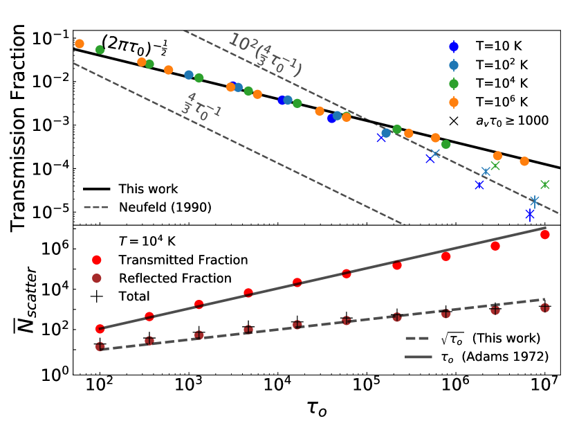
Figure 4: Top: Transmission fraction as a function of $\tau_{0}$ through an externally illuminated homogeneous slab. Simulations are shown for different temperatures and compared with the analytical results. Bottom: mean number of scatterings of transmitted and reflected photons from an externally illuminated slab as a function of optical depth at $T=10^{4}$ K. Solid and dashed lines display the analytical solutions. The behaviour of the entire set of photons is represented with x-markers.

Eq. 6 establishes a linear relation between the hole-to-slab flux ratio $\tilde{f}$ and the side area of the cavity $\tilde{s}$, independent of optical depth. In Fig. 5, the red solid lines represent $\tilde{f}$ obtained from simulations for several values of $\tau_{o}$. Simulations replicate the $\sim\tilde{s}$ trend with a difference of a factor of ten. To compute the simulated $\tilde{f}$, we omitted photons escaping through the hole directly from the emission plane without interacting with the gas (i.e., with $N_{\rm scatter}=0$) since our model does not account for them. For comparison, we also include the previous theoretical prediction $\tilde{f}\sim\tilde{s}\tau_{o}$. It is worth noting that both approaches differ by at least three orders of magnitude, meaning that the previous theoretical approach predicts that most of the flux will come from the hole rather than the slab.

Fig. 5 confirms that: (a) the fraction $\tilde{f}$ varies only slightly with optical depth, (b) $\tilde{f}$ increases linearly with $\tilde{s}$ as expected by Eq. 6, and (c) contrary to previous expectations, the central peak intensity is comparable to the red and blue peaks. In other words, the presence of a large hole does not necessarily imply that all the flux will escape through it.

The present work has some caveats. As mentioned earlier, both the anisotropic and the externally illuminated setups used for this study simplify the highly complicated gas structure in galaxies. We did not address additional factors that alter  Ly$\alpha$ propagation, for instance, the presence of dust, known to absorb radiation and suppress the emergent  Ly$\alpha$ line (Laursen et al., 2009), or outflows, known to change the peaks velocity offset (Bonilha et al., 1979). In future work, we will revisit these caveats and extend our model to different geometries, lines of sight, kinematics, dust content, and channel configurations. We will also discuss using these models to analyse observational data. Note also that the analytic model presented in § 2.2 contains several simplifying assumptions. For instance, we assumed that the mean free path $\lambda_{\rm mfp}$ remains constant despite the frequency redistribution since we assume that photons mainly scatter in the line’s core before escaping in a single excursion at $x\gtrsim_{\rm esc}$. Furthermore, the factor $\alpha$ in Eq. 5 is a first-order approximation that depends on different optical depths. These simplifications lead to the required fudge factor in Eq. 6. However, given the complexity of  Ly$\alpha$ radiative transfer, our analytical model works surprisingly well and can explain the surprising escape behaviour observed.

Figure 5: Fraction of photons escaping through the ionised hole $F_{\rm centre}$ (described in § 4.3) as a function of the size of the hole and with varying optical depth.

5 Discussion & Conclusion

While gas distributions inside galaxies are well known to be highly anisotropic, there is still a lack of systematic studies on the resonant line transfer of  Ly$\alpha$ through such geometries. This is highly surprising given that nature is generally anisotropic.In particular both theoretical (e.g., McKee & Ostriker, 1977) and observational studies (e.g., Martin, 2005) have well established that the gas distribution in the ISM is patchy with a wide variation in HI column densities. Motivated by this, we studied the simplest anisotropic setup: a HI-filled slab with a single, empty hole/channel carved in the neutral gas distribution. Regardless of the setup’s simplicity, the results are counter-intuitive and far from simple. Given the considerable difference in line-centre optical depth between the slab and the hole (up to $\sim 10^{7}$), the naive initial expectation is that most  Ly$\alpha$ photons escape through the empty channel, similar to light passing through the windows instead of the walls (see the discussion in § 2.1). Our numerical results show, in contrast, that only a fraction of photons escape through such a channel.

To explain this dilemma, we developed an analytical model describing  Ly$\alpha$ photons’ general scattering and transmission behaviour. Our findings show that in an externally illuminated slab, photons projected towards the gas undergo a much greater number of scatterings before being reflected. In other words, reflected photons do not bounce out of the slab like ping-pong balls, but penetrate and scatter within the neutral gas before escaping from it. Specifically, we find that the number of scatterings per reflection follows a Lévy Distribution ($\propto N_{\rm scatter}^{-3/2}$ for large $N_{\rm scatter}$). These additional scatterings increase the chances of photons shifting their frequency enough to escape. As a consequence, these extra scatterings lead to a much greater transmission probability $\sim\tau_{0}^{-1/2}$ instead of the currently established and orders of magnitude smaller $\tau_{0}^{-1}$ (Neufeld, 1990).

Our results imply that  Ly$\alpha$ photons are surprisingly much less susceptible to the line-of-sight column densities than previously believed. In other words,  Ly$\alpha$ photons don’t probe only the path of ‘least resistance’ (lowest column density) but rather a more general average of the distribution $p(N_{\rm HI})$. The new corrected transmission probability directly influences emergent  Ly$\alpha$ spectra since photons trace information from more than one escape route instead of only the lowest density one.

In the setup of a slab with a hole,  Ly$\alpha$ spectra trace photons, exiting both the hole (central peak) and the slab (red and blue peaks). The altered picture of  Ly$\alpha$ escape through anisotropic media can explain why triple-peaked spectra, like those in Fig. 2, appear in our simulations instead of single-peaked spectra near the line centre. To quantify the  Ly$\alpha$ radiation that escapes through the hole, we defined the central flux fraction in Eq. 6. We found that the central flux does not depend on the exact column density of the optically thick region but solely on the channel’s size. Furthermore, as indicated by Fig. 5, channels with $\tilde{s}<0.06$ produce spectra with a central peak $\sim 1$ order of magnitude smaller than the blue and red peaks. Under these circumstances, the channel is potentially ‘hidden’ even in a high ($\sim 10^{21}\,{{\mathrm{cm}}}^{-2}$) column density system (see, for example, $\tilde{s}=0.01$ in the middle panel of Fig. 2). Thus,  Ly$\alpha$ could probe a porous ISM even while indicating high column densities with a wide peak separation. This implies, for instance, that observations of  Ly$\alpha$ spectra pointing towards a high column density do not rule out the presence of low HI channels through which LyC can leak. This seems at odds with studies suggesting a clear correlation of the  Ly$\alpha$ peak separation and LyC escape (e.g., Izotov et al., 2021). However, it might be that some of the (small, low-z) galaxies driving this correlation are rather isotropic systems and a population of anisotropic LyC leakers with larger  Ly$\alpha$ peak separation exists.

In summary, our study suggests that  Ly$\alpha$ observables are shaped by average conditions rather than by only extremum statistics and can thus be used to study galaxy formation and evolution in a statistical manner.

Acknowledgements. We thank D. Neufeld for the very useful discussions and encouragement. MG thanks the Max Planck Society for support through the Max Planck Research Group. This research was supported in part by grant NSF PHY-2309135 to the Kavli Institute for Theoretical Physics (KITP).

Data Availability. The data underlying this article will be shared on reasonable request to the corresponding author.

References

- Adams (1972) Adams T. F., 1972, The Astrophysical Journal, 174, 439
- Ahn & Lee (2002) Ahn S.-H., Lee H.-W., 2002, Journal of Korean Astronomical Society, 35, 175
- Barnes et al. (2014) Barnes L. A., Garel T., Kacprzak G. G., 2014, Publications of the Astronomical Society of the Pacific, 126, 969
- Behrens & Braun (2014) Behrens C., Braun H., 2014, Astronomy and Astrophysics, 572, A74
- Bik et al. (2018) Bik A., Östlin G., Menacho V., Adamo A., Hayes M., Herenz E. C., Melinder J., 2018, Astronomy & Astrophysics, 619, A131
- Bonilha et al. (1979) Bonilha J. R. M., Ferch R., Salpeter E. E., Slater G., Noerdlinger P. D., 1979, The Astrophysical Journal, 233, 649
- Chang et al. (2024) Chang S.-J., Arulanantham N., Gronke M., Herczeg G. J., Bergin E. A., 2024, Monthly Notices of the Royal Astronomical Society, 529, 2656
- Cox & Smith (1974) Cox D. P., Smith B. W., 1974, The Astrophysical Journal, 189, L105
- Dahle et al. (2016) Dahle H., et al., 2016, Astronomy and Astrophysics, 590, L4
- Dijkstra (2014) Dijkstra M., 2014, Publications of the Astronomical Society of Australia, 31, e040
- Dijkstra et al. (2006) Dijkstra M., Haiman Z., Spaans M., 2006, The Astrophysical Journal, 649, 37
- Dijkstra et al. (2016) Dijkstra M., Gronke M., Venkatesan A., 2016, The Astrophysical Journal, 828, 71
- Erb et al. (2014) Erb D. K., et al., 2014, The Astrophysical Journal, 795, 33
- Gronke & Dijkstra (2014) Gronke M., Dijkstra M., 2014, Monthly Notices of the Royal Astronomical Society, 444, 1095
- Gronke & Dijkstra (2016) Gronke M., Dijkstra M., 2016, The Astrophysical Journal, 826, 14
- Gronke et al. (2016) Gronke M., Dijkstra M., McCourt M., Oh S. P., 2016, The Astrophysical Journal, 833, L26
- Hansen & Oh (2006) Hansen M., Oh S. P., 2006, Monthly Notices of the Royal Astronomical Society, 367, 979
- Harrington (1973) Harrington J. P., 1973, Monthly Notices of the Royal Astronomical Society, 162, 43
- Hayes et al. (2021) Hayes M. J., Runnholm A., Gronke M., Scarlata C., 2021, The Astrophysical Journal, 908, 36
- Herenz et al. (2017) Herenz E. C., Hayes M., Papaderos P., Cannon J. M., Bik A., Melinder J., Östlin G., 2017, Astronomy and Astrophysics, 606, L11
- Izotov et al. (2018) Izotov Y. I., Worseck G., Schaerer D., Guseva N. G., Thuan T. X., Fricke Verhamme A., Orlitová I., 2018, Monthly Notices of the Royal Astronomical Society, 478, 4851
- Izotov et al. (2021) Izotov Y. I., Worseck G., Schaerer D., Guseva N. G., Chisholm J., Thuan T. X., Fricke K. J., Verhamme A., 2021, Monthly Notices of the Royal Astronomical Society, 503, 1734
- Jaskot et al. (2019) Jaskot A. E., Dowd T., Oey M. S., Scarlata C., McKinney J., 2019, The Astrophysical Journal, 885, 96
- Kakiichi & Gronke (2021) Kakiichi K., Gronke M., 2021, The Astrophysical Journal, 908, 30
- Kim et al. (2023) Kim K. J., et al., 2023, Small Region, Big Impact: Highly Anisotropic Lyman-continuum Escape from a Compact Starburst Region with Extreme Physical Properties, http://arxiv.org/abs/2305.13405
- Laursen et al. (2009) Laursen P., Sommer-Larsen J., Andersen A. C., 2009, The Astrophysical Journal, 704, 1640
- Li & Gronke (2022) Li Z., Gronke M., 2022, Monthly Notices of the Royal Astronomical Society, 513, 5034
- Martin (2005) Martin C. L., 2005, The Astrophysical Journal, 621, 227
- McKee & Ostriker (1977) McKee C. F., Ostriker J. P., 1977, The Astrophysical Journal, 218, 148
- Neufeld (1990) Neufeld D. A., 1990, The Astrophysical Journal, 350, 216
- Neufeld (1991) Neufeld D. A., 1991, The Astrophysical Journal, 370, L85
- Orlitová et al. (2018) Orlitová I., Verhamme A., Henry A., Scarlata C., Jaskot A., Oey M. S., Schaerer D., 2018, Astronomy and Astrophysics, 616, A60
- Ouchi et al. (2020) Ouchi M., Ono Y., Shibuya T., 2020, Observations of the Lyman-$\alpha$ Universe, doi:10.1146/annurev-astro-032620-021859, https://arxiv.org/abs/2012.07960v1
- Rivera-Thorsen et al. (2017) Rivera-Thorsen T. E., et al., 2017, Astronomy and Astrophysics, 608, L4
- Rivera-Thorsen et al. (2019) Rivera-Thorsen T. E., et al., 2019, Science, 366, 738
- Smith et al. (2022) Smith A., et al., 2022, Monthly Notices of the Royal Astronomical Society, 517, 1
- Steidel et al. (2010) Steidel C. C., Erb D. K., Shapley A. E., Pettini M., Reddy N., Bogosavljević M., Rudie G. C., Rakic O., 2010, The Astrophysical Journal, 717, 289
- Vanzella et al. (2020) Vanzella E., et al., 2020, Monthly Notices of the Royal Astronomical Society, 491, 1093
- Verhamme et al. (2006) Verhamme A., Schaerer D., Maselli A., 2006, Astronomy and Astrophysics, 460, 397
- Verhamme et al. (2015) Verhamme A., Orlitová I., Schaerer D., Hayes M., 2015, Astronomy and Astrophysics, 578, A7
- Wisotzki et al. (2016) Wisotzki L., et al., 2016, Astronomy and Astrophysics, 587, A98
- Yang et al. (2016) Yang H., Malhotra S., Gronke M., Rhoads J. E., Dijkstra M., Jaskot A., Zheng Z., Wang J., 2016, The Astrophysical Journal, 820, 130
- Zackrisson et al. (2013) Zackrisson E., Inoue A. K., Jensen H., 2013, The Astrophysical Journal, 777, 39
- Zheng & Wallace (2014) Zheng Z., Wallace J., 2014, The Astrophysical Journal, 794, 116