Analysis of Distributed Optimization Algorithms
on a Real Processing-In-Memory System

Abstract

Machine Learning (ML) training on large-scale datasets is a very expensive and time-consuming workload. Processor-centric architectures (e.g., CPU, GPU) commonly used for modern ML training workloads are limited by the data movement bottleneck, i.e., due to repeatedly accessing the training dataset. As a result, processor-centric systems suffer from performance degradation and high energy consumption. Processing-In-Memory (PIM) is a promising solution to alleviate the data movement bottleneck by placing the computation mechanisms inside or near memory. Several prior works propose PIM techniques to accelerate ML training; however, prior works either do not consider real-world PIM systems or evaluate algorithms that are not widely used in modern ML training.

Our goal is to understand the capabilities and characteristics of popular distributed optimization algorithms on real-world PIM architectures to accelerate data-intensive ML training workloads. To this end, we 1) implement several representative centralized distributed optimization algorithms, i.e., based on a central node responsible for the synchronization and orchestration of the distributed system, on UPMEM’s real-world general-purpose PIM system, 2) rigorously evaluate these algorithms for ML training on large-scale datasets in terms of performance, accuracy, and scalability, 3) compare to conventional CPU and GPU baselines, and 4) discuss implications for future PIM hardware and the need to shift to an algorithm-hardware codesign perspective to accommodate decentralized distributed optimization algorithms.

Our results demonstrate three major findings: 1) Modern general-purpose PIM architectures can be a viable alternative to state-of-the-art CPUs and GPUs for many memory-bound ML training workloads, when operations and datatypes are natively supported by PIM hardware, 2) the importance of carefully choosing the optimization algorithm that best fit PIM, and 3) contrary to popular belief, contemporary PIM architectures do not scale approximately linearly with the number of nodes for many data-intensive ML training workloads. To facilitate future research, we aim to open-source our complete codebase.

1 Introduction

Stochastic Gradient Descent (SGD) [1] is perhaps the most important and commonly deployed optimization algorithm for modern machine learning (ML) training [2, 3, 4]. SGD is the main building block of most centralized and decentralized distributed optimization algorithms that have been introduced to accommodate the continuously increasing demand for scalability and high-performance training of ML models on large-scale datasets.

Training ML models on growing datasets [5, 6, 7] is a time-consuming, costly, compute-intensive, and fundamentally memory-bound workload [8, 9, 10]. The large amount of training data could not fit on the processor’s on-chip memory. As a result, processor-centric architectures (e.g., CPU, GPU) commonly used by the ML community repeatedly need to move training samples between the processor and off-chip memory. This not only degrades performance [11] but is also a major source of the overall system’s energy consumption [12]. This phenomenon is often referred to as the data movement bottleneck [13, 14, 15], which is ubiquitous in data-intensive workloads. ML training and inference are some of the most prominent examples.

Processing-In-Memory (PIM) [14, 15, 16, 17, 18] is one way to alleviate the data movement bottleneck by placing the computation mechanisms inside or near memory. PIM, an idea proposed several decades ago [19, 20], is a compute paradigm that recently gained traction in academia and some commercial systems and prototypes from industry [9, 21, 22, 23, 24, 25, 26, 27, 28, 29, 30, 31].

There are several prior PIM proposals for training ML models [32, 33, 34, 35, 36, 37]. However, none of these prior works provide a comprehensive evaluation on real-world general-purpose PIM architectures. To our knowledge, there is only one prior work [21, 22] on training and evaluating ML models on a real-world PIM system using gradient descent (GD) [38] but unfortunately, GD-based algorithms are not widely used in modern machine learning. Our work is orthogonal with this prior work as, in our study, we target training algorithms and techniques commonly used for distributed machine learning. We focus on popular SGD-based algorithms due to their effectiveness, simplicity, and generalization performance [39].

Our goal in this paper is to understand the capabilities and characteristics of popular distributed optimization algorithms on real-world PIM architectures to accelerate data-intensive ML training workloads. To do so, we implement and rigorously evaluate $12$ representative ML training workloads, commonly used in the ML community, on UPMEM’s real-world PIM architecture. We choose UPMEM’s PIM system for our study because it is the first commercial general-purpose PIM architecture [40, 41, 42], introduced by the UPMEM company. First, we implement and investigate all combinations of 1) three distributed optimization algorithms that specifically take into account the close resemblance of UPMEM’s PIM system to a distributed system [43], Mini-Batch Stochastic Gradient Descent with Model Averaging (MA-SGD) [44, 45], Mini-Batch Stochastic Gradient Descent Gradient Averaging (GA-SGD) [46, 47], and the communication-efficient distributed Alternating Direction Method of Multipliers (ADMM) algorithm [48], 2) two popular and representative linear binary classification models, Logistic Regression (LR) and Support Vector Machine (SVM), and 3) two large-scale datasets, YFCC100M-HNfc6 and Criteo [49, 50]. Second, we rigorously evaluate all combinations of these algorithms, models, and datasets in terms of performance, accuracy, and scalability. Third, we compare the training speed and test set inference accuracy of PIM to state-of-the-art CPU (2x AMD EPYC 7742 CPU 64-core processor) and GPU (NVIDIA A100) baselines. Fourth, we discuss implications for future PIM hardware and the need to shift to an algorithm-hardware codesign perspective to accommodate decentralized distributed optimization algorithms.

Our results demonstrate three major findings: 1) PIM can be a viable alternative to state-of-the-art CPUs and GPUs for many data-intensive ML training workloads when operations and datatypes are natively supported by PIM hardware, 2) the importance of carefully choosing the optimization algorithm that best fits PIM, and 3) contrary to popular belief, we uncover scalability challenges in terms of statistical efficiency of ML models trained on PIM. For instance, for training SVM with GA-SGD, PIM is $1.94$x faster/$2.43$x slower compared to the CPU baseline, and $3.19$x/$10.65$x faster compared to baseline SGD on the GPU architecture on the YFCC100M-HNfc6/Criteo dataset while achieving similar accuracy. Second, training SVM with the ADMM algorithm using PIM, we observe speedups of $1.39$x/$31.82$x compared to GA-SGD at the cost of a reduction of the test accuracy/ROC AUC score (accuracy metric; see §4.2 for more details) by only $1.009$x/$1.014$x on PIM for the YFCC100M-HNfc6/Criteo dataset. As a final example, in our strong scaling (see §5 for more details) experiments of the YFCC100M-HNfc6/Criteo dataset, training LR with ADMM using PIM, we observe speedups of $7.43$x/$3.85$x while the achieved test accuracy/ROC AUC score decreases from $95.46$%/$0.74$ to $92.17$%/$0.718$, as we scale the number of nodes from $256$ to $2048$.

This paper makes the following key contributions:

• To our knowledge, we are the first to implement, analyze, and train linear ML models using realistic and communication-efficient distributed optimization algorithms on a real-world PIM architecture and evaluate on the two large-scale datasets YFCC100M-HNfc6 and Criteo.

• We present the design space covering the design choices of various algorithms, models, and workloads for ML training on PIM.

• We demonstrate PIM’s scalability challenges in terms of statistical efficiency and discuss implications for hardware design to accommodate decentralized parallel optimization algorithms shown to be more robust toward scaling and the need to shift towards an algorithm-hardware codesign perspective in the context of ML training using PIM.

• To facilitate future research, we aim to open-source our complete codebase.

2 Background & Motivation

We provide a brief introduction on ML training, Models, Algorithms, and Regularization (§2.1). We elaborate on UPMEM’s Processing-In-Memory (PIM) system (§2.2), the first real-world general-purpose PIM hardware architecture we study in this paper. For general PIM background and discussion of many works in the field, we refer the reader to [15, 14, 16]. We conclude this section with our Motivation (§2.3).

2.1 ML Training, Models, Algorithms & Regularization

ML Training. The goal of ML training is to find an optimal ML model $w\in\mathbb{R}^{n}$ minimizing a loss function $L\colon\text{argmin}_{w}\frac{1}{N}\sum_{i=1}^{N}L(x_{i},y_{i},w)$ over a training dataset $\mathcal{D}=\{(x_{i},y_{i})\}_{i=1}^{N}$, where $x_{i}\in\mathbb{R}^{n}$ is referred to as feature vector, and $y_{i}\in\mathbb{R}$ as label of the $i^{th}$ sample [4].

Models. We consider two linear binary classification models commonly used for convex optimization tasks: 1) Logistic Regression (LR) with Binary Cross Entropy Loss (BCE), and labels $y_{i}\in\{0,1\}$. 2) Support Vector Machines (SVM) with Hinge Loss, and labels $y_{i}\in\{-1,1\}$ [51]. Each model consists of a linear layer and a bias.

Algorithms. In this work we consider three centralized distributed optimization algorithms for training both LR and SVM: 1) Mini-Batch Stochastic Gradient Descent with Model Averaging (MA-SGD) [44, 45], 2) Mini-Batch Stochastic Gradient Descent Gradient Averaging (GA-SGD) [46, 47], and 3) Distributed Alternating Direction Method of Multipliers (ADMM) [48]. These algorithms are based on a parameter server, i.e. a central node, that is responsible for synchronization and updating the global model, and several workers among which the training dataset is evenly partitioned.

In the case of MA-SGD, every worker trains a local model using the optimization algorithm SGD [1] in parallel. Each worker processes several mini-batches, updating its local model before synchronization on the parameter server where the models are averaged. Then, the averaged model, i.e., the global model, is broadcast back to the workers, and each worker continues training with SGD starting from the global model. There exists a one-shot averaging [44, 45] variant of the MA-SGD algorithm, where models are averaged after each worker has processed its entire partition of the training data. Although one-shot averaging reduces communication, it has been shown that increasing the model averaging frequency admits a higher convergence rate [52, 53]. Therefore, in this work, we analyze the behavior of MA-SGD, where the models are averaged after each local worker has processed exactly one mini-batch.

In contrast, GA-SGD distributes each batch among all workers. Each worker runs SGD, computes the gradients for a fraction of the batch, and communicates the gradient with the parameter server, where the gradients are averaged and the global model is updated. Subsequently, the global model is communicated with the workers, and the next batch is processed. For GA-SGD and MA-SGD, we will refer to one global epoch once the whole training dataset has been processed.

The distributed ADMM algorithm follows a decomposition-coordination procedure, dividing a convex optimization problem into smaller local subproblems distributed among workers [4, 48]. Each worker solves its subproblem, e.g. with SGD until convergence. Next, the local models are communicated with the parameter server, where the global model and auxiliary variables that help lead the workers to a consensus are computed. Each worker continues training with its local model after the synchronization step. For ADMM, we will refer to one global epoch once the synchronization step on the parameter server has been completed.

Regularization. We use standard regularization techniques to achieve lower generalization error. For MA-SGD and GA-SGD, we add a $\ell_{2}$ regularization term to the loss functions of the LR and SVM models. For ADMM, we include $\ell_{2}$ regularization for the SVM loss function, while we include $\ell_{1}$ regularization for LR. By including $\ell_{1}$ regularization for LR ADMM, the dual optimization problem admits a closed-form solution similar to SVM ADMM with $\ell_{2}$ regularization [48].

2.2 UPMEM PIM System Architecture

Fig. 1 illustrates the high-level system organization of an UPMEM PIM-enabled system and the hardware architecture of an UPMEM PIM chip. The system consists of a regular host CPU which we will refer to as parameter server ❶, conventional main memory modules ❷, and UPMEM PIM memory modules ❸. Each UPMEM PIM memory module contains two ranks ❹. Each rank has 8 UPMEM PIM chips ❺. Inside each chip, there are 8 banks. Each bank contains 1) a 64MB DRAM array called MRAM ❻, and 2) a general-purpose DRAM Processing Unit (DPU) ❼.

Figure 1: High-level system organization of an UPMEM PIM-enabled system and the hardware architecture of an UPMEM PIM chip.

The MRAM implements a standard JEDEC DDR4 DRAM interface that can be accessed by the host CPU. The DPU has an SRAM Instruction Memory, a 64KB SRAM Working Memory (WRAM), and an in-order fine-grained multi-threaded pipeline with 11 stages and support 24 hardware threads. It implementes a 32-bit RISC-based instruction set architecture (ISA) with native support for 32-bit integer additions/subtractions and 8-bit integer multiplications. Other more complex arithematic operations (e.g., integer divisions and floating-point operations) are emulated through software. The DPU does not have a cache, but uses the WRAM as a scratchpad memory [42, 41].

Each DPU has exclusive access to its MRAM (with respect to other DPUs) through a high-bandwidth (up to 0.7GB/s) internal data bus  [9, 21]. There is no direct communication channels among DPUs within an UPMEM PIM chip. All inter-DPU communications are done through the host CPU (i.e., the CPU first gathers data from the DPUs’ MRAM into the system’s main memory, and then distributes the data from main memory to the DPUs’ MRAM).

PIM Programming and Execution Model. DPU programs are written in the C programming language with the UPMEM SDK [54] and runtime libraries. The execution model of DPU is based on the Single-Program Multiple-Data (SPMD) paradigm. Each DPU runs multiple (up to 24) software threads, called tasklets, which execute the same code but operates on different data. Each tasklet has its own control flow, independent from other tasklets. Tasklets are assigned to DPUs statically by the programmer during compile-time. Tasklets assigned to the same DPU share MRAM and WRAM [9, 21].

2.3 Motivation

SGD is one of the most important optimization algorithms and the basis of many distributed optimization algorithms. However, SGD is memory-bound [55, 56, 57, 58, 59], which poses a fundamental challenge for processor-centric architectures (e.g., CPU, GPU). SGD’s memory-boundedness is attributed to increasing data size leading to decreased cache efficiency resulting in performance degradation [55, 60, 61]. The increasing discrepancy in performance between fast processors and slow memory units exacerbates this problem [21]. PIM is one way to alleviate the data movement bottleneck and is a promising candidate for various ML training workloads.

There are several prior proposals on PIM acceleration for ML training [32, 33, 34, 35, 36, 37]. However, none of these prior works provide a comprehensive evaluation on real-world general-purpose PIM architectures. To our knowledge, there is only one prior work [21, 22] on training and evaluating ML models on a real-world PIM system using gradient descent (GD) [38] with gradient averaging. Our work differs from prior work as, in our study, we target optimization algorithms and techniques commonly used for distributed machine learning. We specifically take into account that UPMEM’s PIM architecture resembles a centralized distributed system [43].

To show the importance of carefully choosing the optimization algorithm that best fits PIM architectures, we analyze key differences in communication patterns of distributed algorithms on UPMEM’s PIM system. We consider ML training using $2048$ DPUs on the Criteo dataset in the following. In Fig. 2, we show the per global epoch bandwidth between PIM and the parameter server and within PIM, i.e., aggregated bandwidth between MRAM and WRAM (first column). We illustrate the per global epoch total data movement between PIM and the parameter server and within PIM (second column). For MA-SGD/ADMM, the batch size is $2$K; for GA-SGD, it is $262$K.

Figure 2: Per global epoch comparison of various communication pattern metrics of all combinations of models and algorithms for the Criteo dataset.

We make two major observations. First, the bandwidth gap between PIM and the parameter server and within PIM is huge. For instance, for the model LR, we observe that the bandwidth within PIM for MA-SGD/GA-SGD/ADMM is $64.54$x/$88.35$x/$85.22$x higher than the communication bandwidth between PIM and the parameter server. Second, the absolute data movement between PIM and the parameter server is very high. For instance, for LR, the algorithms MA-SGD/GA-SGD exhibit $64.01$x/$1536.16$x higher absolute data movement for expensive communication between PIM and the parameter server per global epoch compared to ADMM.

We conclude that algorithms with little expensive communication between PIM and the parameter server should be chosen. It is necessary to tailor implementations of distributed optimization algorithms to enable the training of ML workloads on current PIM hardware architecture because these novel PIM architectures are fundamentally different from processor-centric architectures [9].

3 Implementation

This section provides a high-level overview of our PIM Implementation (§3.1), Baseline Implementations (§3.2) and discuss Implementation Details (§3.3).

3.1 PIM Implementation

Fig. 3 illustrates the high-level control flow of training ML models using the UPMEM PIM system. First, the host CPU, i.e., the parameter server, initializes the DPUs by sending the DPU program to the DPUs and assigns tasklets to DPUs. Then, the host partitions the whole training dataset and distributes them to the DPUs. Each DPU is statically assigned a partition of the training dataset consisting of multiple mini-batches. The corresponding partitions are transferred from the host to the DPU only once and will remain on the same DPU during the entire training process. For all ML training workloads, we use $16$ tasklets to utilize the multi-threaded pipeline fully and improve latency [9]. Once the DPU kernels have completed computation of the local model for MA-SGD/ADMM, or in the case of GA-SGD, the gradient, these parameters are collected by the host CPU. The host aggregates the intermediate states and generates a global state following a specific pattern depending on the distributed optimization algorithm considered. Subsequently, the host communicates the global state with the DPUs and continues training by invoking the DPU kernels. Communication patterns and the generation of a global state of the statistics vary for each algorithm, as described in §2.1. Each DPU is a worker in our implementation.

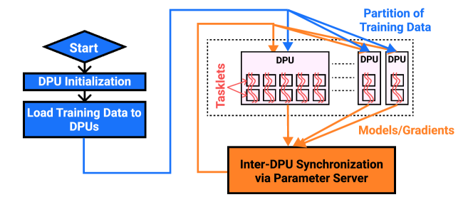
Figure 3: High-level control flow for parallel optimization algorithms on UPMEM’s PIM architecture.

3.2 Baseline Implementations

We evaluate and compare our PIM implementation to state-of-the-art CPU and GPU. We fine-tune and optimize the baseline implementations.

CPU Baseline. We use a distributed PyTorch implementation. We implement MA-SGD, GA-SGD, and ADMM and train LR and SVM models. Implementations follow an AllReduce communication pattern. We consider each CPU thread as a worker.

GPU Baseline. We use PyTorch for the GPU implementation. We only implement mini-batch SGD on the GPU because PyTorch does not provide a way to limit the amount of GPU resources the kernels use, causing model averaging to be serialized on a single GPU, indicating that there is little interest by the ML community for support of distributed optimization algorithms on a single GPU. Training of deep neural networks is a workload better suited for GPUs and in distributed settings models are commonly trained on a cluster of GPUs. Training models on a multi-GPU system is out of the scope of this work.

3.3 Implementation Details

In the following, we lay out other implementation details and explain the rationale of our design choices:

PIM Implementation of Arithmetics. Training of LR involves computing the exponential function to evaluate the sigmoid. Since UPMEM’s PIM architecture does not support transcendental functions, we use efficient LUT-based methods [62, 21, 63] for computation. LUTs are fast [62, 63] but incur significant storage overhead (in our case, $4$MB of MRAM per DPU). Additionally, expensive 64-bit integer multiplications must be used to avoid overflows, e.g., to compute the dot product of model parameters and train sample features, both represented in a 32-bit fixed-point format.

Data Format. We conduct ML training on PIM on quantized [64, 65, 66, 67] train data and models, i.e., both represented in a 32-bit fixed-point format, because UPMEM’s PIM system does not natively support floating-point operations. We use a floating-point format, i.e., FP32, for our CPU and GPU baselines because 1) CPUs and GPUs natively support it and 2) it provides higher accuracy. The main reason for this choice is that we want to focus on fundamental differences in memory bandwidth. Additionally, the industry has a high interest in PIM systems [27]. Hence, it is likely that future PIM architectures will natively feature floating-point operations.

Hyperparameter Tuning. We tune the learning rates and regularization terms for all workloads this paper evaluates. We will make all tested hyperparameters public joint with an open-source repository of our complete codebase.

Batch Size. For training models on YFCC100M-HNfc6, we consider batch sizes $8$, $16$, $32$, and $64$ for MA-SGD/ADMM and $4$K, $8$K, $16$K, and $32$K for GA-SGD. For training models on Criteo, we consider batch sizes $1$K, $2$K, $4$K, and $8$K for MA-SGD/ADMM, and $131$K, $262$K, $524$K, and $1048$K for GA-SGD. We use different batch sizes for Criteo due to its orders of magnitude larger number of samples in the training dataset (4.2).

4 Methodology

In this section, we describe the system configurations (§4.1), and datasets (§4.2) used in this paper.

4.1 System Configurations

Table 1 shows the system configuration of 1) the UPMEM PIM system, 2) the CPU baseline system, and 3) the GPU baseline system that we evaluate the ML training workloads on.

Table 1: PIM and baseline system configurations

UPMEM PIM System
Processor	2x Intel Xeon Silver 4215 8-core processor @ 2.50GHz
Main Memory	$256\text{\,}\mathrm{GB}$ total capacity DDR4, 4$\times{}$$64\text{\,}\mathrm{GB}$ DDR4 registered dual in-line memory modules (RDIMMs)
PIM-Enabled Memory	$160\text{\,}\mathrm{GB}$ total capacity 20$\times{}$$8\text{\,}\mathrm{GB}$ UPMEM PIM modules, 2560 DPUs, 2 ranks per module, 8 chips per rank, 8 DPUs per chip $350\text{\,}\mathrm{MHz}$ DPU clock frequency
CPU Baseline System
Processor	2x AMD EPYC 7742 64-core processor @ 2.25GHz
Main Memory	$1\text{\,}\mathrm{TB}$ total capacity 32$\times{}$$32\text{\,}\mathrm{GB}$ DDR4 registered dual in-line memory modules (RDIMMs)
GPU Baseline System
Processor	2x Intel Xeon Gold 5118 12-core processor @ 2.30GHz
Main Memory	$512\text{\,}\mathrm{GB}$ total capacity DDR4, 16$\times{}$$32\text{\,}\mathrm{GB}$ DDR4 registered dual in-line memory modules (RDIMMs)
GPU	1$\times{}$ NVIDIA A100 (PCIe, $80\text{\,}\mathrm{GB}$)

4.2 Datasets

We consider two large-scale datasets:

1) YFCC100M-HNfc6 [49] consists of 97M samples with features extracted by a deep convolutional neural network from the YFCC100M multimedia dataset [68]. Each sample consists of $4^{\prime}096$ floating-point dense features and a collection of tags. We randomly sample data points with the tag "outdoor", treating them as positive labels and sample the same number of data points with the tag "indoor", treating them as negative labels, turning this subset into a binary classification task. We apply standard normalization to each feature column, and for our implementation on the DPU architecture, we additionally quantize the normalized dataset into a 32-bit fixed-point format. The total size of model parameters is $4$KB.

2) Criteo 1TB Click Logs [50] preprocessed by LIBSVM [69] consisting of approximately $4.37$ billion high-dimensional sparse samples with $1$M features. Criteo is a popular click-through rate prediction dataset. Data points labeled "click" are treated as positive and "no-click" as negative labels. The dataset has been collected over $24$ days and is highly imbalanced, with only $0.034$% of data points being "clicks". To construct the training dataset, we randomly sample from day $0$ to $22$ while maintaining the ordering only among days. We hold out the entire day $23$ and use it as a test dataset for all our experiments. Each data point consists of a label and $39$ categorical features representing a sparse embedding in a $1$M-dimensional feature space. Note, while data points only consist of $40$ parameters, the models/gradients consist of $1$M variables and, therefore, incur a significantly higher communication overhead compared to YFCC100M-HNfc6. We use the metric ROC AUC score to accurately assess the generalization capabilities of models trained on Criteo due to its imbalanced data distribution. The total size of the model parameters is $4$MB.

Table 2 summarizes the dataset configurations used in our experiments for scaling analysis and comparison to CPU and GPU.

Table 2: Dataset configuration

YFCC100M-HNfc6
# Workers	# Train samples	Train size (GB)	# Test samples	Test size (GB)
256 DPUs	851’968	13.96	212’992	3.49
512 DPUs	1’703’936	27.92	425’984	6.98
1024 DPUs	3’407’872	55.83	851’968	13.96
2’048 DPUs	6’815’744	111.67	1’703’936	27.92
128 CPU threads	6’815’744	111.67	1’703’936	27.92
1 GPU	6’815’744	111.67	1’703’936	27.92
Criteo
# Workers	# Train samples	Train size (GB)	# Test samples	Test size (GB)
256 DPUs	50’331’648	8.05	178’236’537	28.52
512 DPUs	100’663’296	16.11	178’236’537	28.52
1’024 DPUs	201’326’592	32.21	178’236’537	28.52
2’048 DPUs	402’653’184	64.42	178’236’537	28.52
128 CPU threads	402’653’184	64.42	178’236’537	28.52
1 GPU	402’653’184	64.42	178’236’537	28.52

5 Evaluation

We evaluate ML training of 1) dense models on the YFCC100M-HNfc6 dataset (§5.1), and 2) high-dimensional sparse models on the Criteo 1TB Click Logs dataset in subsection (§5.2).

For both datasets, we focus our analysis of our experiments as follows:

• PIM Performance Breakdown. To understand key characteristics of distributed machine learning on UPMEM’s PIM system, we break the training time of one global epoch down into communication/synchronization between the parameter server and PIM, PIM computation time, and PIM data movement time, i.e., time spent moving data between MRAM and WRAM.

• Algorithm Selection. To show the importance of carefully choosing the algorithm that best fits an architecture, we compare test accuracy and total training time for various models, algorithms, and architecture.

• Batch Size. We study the impact on performance in terms of total training time and the generalization capabilities of the trained models for varying batch sizes for the PIM and CPU architecture.

• Scaling. We explore two different scaling variants to assess the impact of scaling on total training time and accuracy for PIM. 1) Weak Scaling. We increase the number of DPUs considered in our experiments while the train dataset size is increased accordingly. 2) Strong Scaling. We fix the training dataset size that fits on the smallest number of DPUs, i.e., $256$ DPUs. Specifically, the training dataset remains unchanged as we scale the number of DPUs.

5.1 Evaluation of YFCC100M-HNfc6

PIM Performance Breakdown. In Fig. 4, we study the training time for one global epoch (y-axis) and breakdown of the per global epoch execution time into communication/synchronization between the parameter server and PIM, PIM computation time, and time spent moving data between MRAM and WRAM (x-axis). For MA-SGD and ADMM, we set the batch size to $8$. For GA-SGD, we fix the batch size to $4$K.

Figure 4: Per global epoch performance breakdown.

Obsv. 1. Communication and synchronization between the parameter server and PIM is a bottleneck for MA-SGD/GA-SGD.

For instance, LR MA-SGD/GA-SGD communication and synchronization among the parameter server and PIM requires $56.0$x/$223.3$x more time compared to ADMM. Here, we observe that communication-efficient optimization algorithms such as ADMM improve performance.

Obsv. 2. For all combinations of optimization algorithms and models, computation dominates training time on PIM.

For instance, for LR/SVM MA-SGD on PIM spends $26.75$x/$14.05$x more time on computation than moving data between MRAM and WRAM. That PIM spends less time on computation for SVM than LR is unsurprising because SVM has lower computational complexity.

3 Takeaway 1. PIM is less suitable for ML models and optimization algorithms that 1) require much communication/synchronization among the parameter server and PIM, and 2) are compute-bound.

3

Algorithm Selection. In Fig. 5, we study test accuracy (y-axis), and total training time (x-axis) for $10$ global epochs with different models as columns. PIM with $2048$ DPUs (first row of plots), the CPU architecture with $128$ CPU threads (second row of plots), and the GPU architecture (third row of plots). For the algorithms MA-SGD and ADMM, we set the batch size to $8$. For GA-SGD and baseline SGD, the batch size is fixed to $4$K.

Figure 5: Comparison on various models, algorithms, and architectures. We study test accuracy and total training time for $10$ global epochs.

Obsv. 3. MA-SGD and ADMM have similar performance in terms of total training time and achieved accuracy on PIM. On the CPU architecture, ADMM significantly outperforms MA-SGD in terms of total training time.

For example, for LR, we observe a speedup of $1.51$x/$39.79$x with ADMM compared to MA-SGD on PIM/CPU architecture. The higher speedup on the CPU can be attributed to the smaller number of workers compared to PIM and, therefore, less communication overhead compared to PIM. Additionally, a CPU thread processing $8$ samples per batch before communication is too small. However, for test accuracy, it is desirable to consider smaller batch sizes, as we will discuss in Fig. 6.

Obsv. 4. GA-SGD is slower than ADMM for all configurations of LR, SVM, PIM, and CPU architecture.

For instance, for SVM ADMM, we observe speedups of $3.19$x compared to GA-SGD on PIM and $4.45$x on the CPU architecture. This is a result of efficient communication for ADMM, since local models are collected only after each DPU/CPU thread has processed its complete partition of the training dataset while for GA-SGD gradients are communicated for each gradient step. This might be acceptable for small, dense models since only a small amount of data needs to be communicated. However, scaling the model would introduce a major bottleneck due to increased communication overhead. The speedup gap between PIM and the CPU architectures stems from the larger number of workers for the DPU architecture ($2048$ workers) compared to the CPU architecture ($128$ workers) because for a fixed batch size, one CPU-tread processes more data points compared to one DPU. Additionally, more workers directly leads to more local gradients to be communicated with the parameter server.

Obsv. 5. GA-SGD on PIM outperforms GA-SGD on the CPU architecture and SGD on the GPU architecture for both LR and SVM.

GA-SGD on PIM achieves speedups of $1.62$x/$1.94$x for LR/SVM over the CPU architecture, $2.67$x/$3.19$x for LR/SVM over the GPU running SGD. A possible explanation for these speedups is that per CPU thread, there is not enough work before synchronization with the parameter server (Obsv. 5.1), and the batch size is too small on the GPU. The speedup gap between LR and SVM results from SVM’s lower computational complexity compared to LR, and therefore, SVM is faster than LR on PIM in general.

Obsv. 6. ADMM is faster on PIM for SVM compared to the CPU. For LR, the CPU is faster.

For SVM ADMM, we observe speedups of $1.39$x on PIM compared to the CPU architecture. In contrast, for LR with ADMM we notice a slowdown by a factor of $1.33$x on PIM compared to the CPU architecture. This is unsurprising since the training of SVM on PIM requires less computation and no lookup to approximate the sigmoid function compared to LR.

3 Takeaway 2. PIM is a viable alternative to CPUs and GPUs for training small dense models on large-scale datasets.

3

Batch Size. In Fig. 6, we compare the total training time (y-axis) for 10 global epochs (first row of plots), test accuracy reached in the last global epoch (y-axis) (second row of plots), and varying batch size (x-axis). For the column plots, we illustrate a fixed combination of the model and optimization algorithm. Each subplot compares PIM with $2048$ DPUs and the CPU architecture with $128$ CPU threads for every batch size.

Figure 6: Impact on performance for varying batch size in terms of total training time for $10$ global epochs and test accuracy reached in the last global epoch.

Obsv. 7. As batch size decreases, PIM exhibits less performance degradation compared to CPU for MA-SGD and ADMM.

When batch size decreases from $64$ to $8$, the total training time of SVM MA-SGD on PIM increases by $2.01$x from $75.28$s to $151.36$s, compared to the CPU, where the total training time increases by $6.96$x from $536.30$s to $3730.55$s. This is unsurprising since larger batch sizes directly result in less communication. The reason for the high speedup on the CPU is discussed in Obsv. 5.1. For LR ADMM, the total training time increases by $1.02$x on PIM, compared to $2.10$x on the CPU, respectively. This is because the local model update on PIM is not significantly more compute-intensive and only requires reading the gradient into WRAM compared to a single gradient step. On the CPU side, the slowdown likely stems from polluted caches due to the local model and the gradient to be loaded into the cache with an increased frequency of model updates for smaller batch sizes. We observe that accuracy increases as batch size decreases from $64$ to $8$, e.g., for SVM MA-SGD, the test accuracy increases from $92.84$% to $95.92$% on PIM and from $94.83$% to $96.51$% on the CPU. This increase arises from the famous bias-variance tradeoff [70] when training ML models, i.e., we want to introduce variance by increasing the batch size until we observe a drop in accuracy. Note, that SGD-based algorithms admit unbiased gradient estimates [51]. The discrepancy in test accuracy between PIM and CPU stems from the quantization of the training data and the model and a larger number of models on PIM.

Obsv. 8. Both PIM and the CPU architecture benefit from larger batch sizes for GA-SGD.

Only for GA-SGD, for both PIM and the CPU architecture, do we observe a significant reduction in total training time as we increase the batch size, while jointly, the test accuracy only slightly degrades. This behavior is explained by the reduction of communication for larger batch sizes since each DPU/CPU thread can process more samples before gradients need to be collected and the model is updated. GA-SGD’s test accuracy is less sensitive to increasing batch size because GA-SGD has only one model. We will delve into more detail about how the number of models impacts convergence rates when we discuss our scaling results.

3 Takeaway 3. PIM has benefits for 1) models that require smaller batch sizes, and 2) algorithms that minimize inter-DPU communication.

3

Scaling. In Fig. 7, we compare the total training time (y-axis) for $10$ global epochs (first row of plots), test accuracy reached in the last global epoch (y-axis) (second row of plots), and analyze different optimization algorithms (x-axis). We study the models LR (first column of plots) and SVM (second column of plots). For each subplot, the number of DPUs ($256$, $512$, $1024$, and $2048$) is increased while the train dataset size is scaled accordingly (weak scaling). For MA-SGD and ADMM, we fix the batch size to $8$. For GA-SGD, we set the batch size to $8$K.

Figure 7: Impact of weak scaling on total training time for $10$ global epochs and test accuracy.

Obsv. 9. PIM has good weak scalability with ADMM but bad weak scalability with MA-SGD and GA-SGD in terms of total training time.

As an example, for SVM ADMM/MA-SGD, we observe an increase of total training time by $1.08$x/$1.75$x, while the achieved test accuracy only changes very slightly as we scale from $256$ to $2048$ DPUs. The speedup gap is attributed to the slightly higher communication overhead for small, dense models as we scale the number of workers.

Obsv. 10. Only GA-SGD can profit from a larger training dataset when the number of DPUs is scaled in terms of test accuracy.

For SVM GA-SGD, we observe an increase in total training time by $2.05$x, while the achieved test accuracy increases from $94.15$% to $96.17$% as we scale the number of DPUs from $256$ to $2048$. The slowdown stems from higher communication overhead when training with more DPUs. For GA-SGD, when we increase the number of models, each DPU processes fewer samples per batch, exacerbating the communication overhead.

In Fig. 8, we use the same experiment setting as in Fig. 7, except that, we fix the train dataset size as we scale the number of DPUs (strong scaling).

Figure 8: Impact of strong scaling on total training time for $10$ global epochs and test accuracy.

Obsv. 11. PIM has good strong scalability in terms of total training time, but bad in accuracy.

As an example, for LR ADMM/MA-SGD, we observe a speedup of $7.43$x/$5.47$x, while the achieved test accuracy decreases from $95.46$%/$95.70$% to $92.17$%/$92.73$%, as we scale from $256$ to $2048$ DPUs. In contrast, for LR GA-SGD, we observe a speedup of total training time by $5.22$x, while the achieved test accuracy only slightly improves as we scale the number of DPUs from $256$ to $2048$. Therefore, the communication-efficient ADMM algorithm achieves a higher speedup compared to MA-SGD/GA-SGD. The observed reduction in test accuracy for a larger number of DPUs, i.e., directly corresponding to a larger number of models, when training ML models with MA-SGD/ADMM might be more surprising. Intuitively, more workers increase staleness as each worker has its own local model before synchronization with the parameter server. For a theoretical analysis of this phenomenon of how the number of workers affects the convergence rate, we refer the reader to [71]. Other works also make this empirical observation that convergence becomes slower as the number of workers is scaled [72, 73]. However, these papers consider a substantially smaller number of workers.

3 Takeaway 4. PIM’s scalability potential for ML training workloads is limited by its lack of inter-DPU communication.

3

5.2 Evaluation of Criteo

PIM Performance Breakdown. In Fig. 9, we compare the training time for one global epoch (y-axis), and breakdown of the per global epoch execution time into communication / synchronization between the parameter server and PIM, PIM computation time, and time spent moving data between MRAM and WRAM (x-axis). For MA-SGD and ADMM, we set the batch size to $2$K. For GA-SGD, we fix the batch size to $262$K.

Figure 9: Per global epoch performance breakdown.

Obsv. 12. Communication and synchronization between the parameter server and PIM is a bottleneck for MA-SGD/GA-SGD.

For instance, LR MA-SGD/GA-SGD communication and synchronization among the parameter server and PIM requires $25.10$x/$640.35$x more time compared to ADMM. This coincides with Obsv. 5.1 for the YFCC100M-HNfc6 dataset.

Obsv. 13. For MA-SGD/ADMM, both LR and SVM computation dominates training time on PIM. For GA-SGD, data movement on PIM dominates total training time.

As an example, LR/SVM MA-SGD on PIM spends $6.38$x/$2.46$x more computation time than moving data between MRAM and WRAM. That PIM spends less time on computation for SVM than LR is unsurprising because SVM has lower computational complexity. In contrast to our Obsv. 5.1 for the YFCC100M-HNfc6, for Criteo, for SVM GA-SGD PIM spends $14.29$x more time on moving data between MRAM and WRAM compared to computation. This is a direct result of having to sequentially read the complete gradient into WRAM for the gradient update and subsequently back to MRAM. For Criteo, we can take advantage of larger individual data transfers that are more efficient compared to YFCC100M-HNfc6. Most of the computation of updating the model is offloaded to the parameter server.

3 Takeaway 5. PIM is less suitable for training high-dimensional sparse models and optimization algorithms that 1) require a lot of communication/synchronization among the parameter server and PIM, and 2) are compute-bound.

3

Algorithm Selection. In Fig. 10, we study the ROC AUC score (y-axis), and total training time (x-axis) for 10 global epochs with different model types as columns. PIM with $2048$ DPUs (first row of plots), the CPU architecture with $128$ CPU threads (second row of plots). For the algorithms MA-SGD, and ADMM we set batch size to $2$K. For GA-SGD, and baseline SGD the batch size is fixed to $524$K. For the GPU architecture, we only report a per batch speedup comparison to PIM with GA-SGD (Obsv. 5.2) because training of Criteo’s high-dimensional sparse model with baseline SGD is very slow on the GPU.

Figure 10: Comparison on various models, algorithms, and architectures. We study the ROC AUC score and total training time for $10$ global epochs.

Obsv. 14. ADMM outperforms MA-SGD for both LR and SVM on PIM. On the CPU architecture, ADMM outperforms MA-SGD in terms of total training time; however, it has a lower ROC AUC score.

Training on the sparse dataset Criteo, for LR/SVM ADMM, we observe a speedup of $4.40$x/$7.24$x on PIM and $1.70$x/$1.64$x on the CPU architecture compared to MA-SGD. The speedup gap between LR/SVM on PIM stems from SVM having lower computational complexity and due to communication overhead of MA-SGD dominating the total training time, while on the CPU architecture computational complexity does not significantly affect training time.

Obsv. 15. MA-SGD and ADMM significantly outperform GA-SGD for both LR and SVM on PIM. On the CPU architecture, ADMM outperforms GA-SGD only in terms of total training time. In contrast to PIM, on the CPU architecture, MA-SGD is slightly slower than GA-SGD but achieves a higher ROC AUC score.

For instance, for SVM ADMM, we observe speedups of $31.82$x/$1.41$x compared to GA-SGD at the cost of a reduction of the ROC AUC score by $1.014$x/$1.007$x on the PIM/CPU architecture. The speedup gap between the PIM and CPU architecture for GA-SGD is exacerbated since, for PIM, we have more workers, and therefore, more intermediate gradients need to be communicated over the slow channel between PIM and the parameter server. For SVM MA-SGD, we observe speedups of $4.39$x at the cost of a reduction of the ROC AUC score by $1.02$x on PIM compared to GA-SGD. In contrast, on the CPU architecture, for SVM MA-SGD we observe a slowdown of $1.16$x and an increase of the ROC AUC score by $1.01$x. The increase in training time on the CPU architecture for MA-SGD compared to GA-SGD is a result of that for MA-SGD, each CPU thread needs to read its gradient into cache and update the model followed by communication of the models, while for GA-SGD, the intermediate gradients are communicated directly, and only a single model is updated. Additionally, each CPU thread processes the same number of samples for MA-SGD and GA-SGD.

Obsv. 16. GA-SGD on the CPU architecture outperforms GA-SGD on PIM and the GPU architecture.

GA-SGD on the CPU architecture achieves speedups of $2.75$x/$2.43$x for LR/SVM over the PIM architecture. This observation differs from our Obsv. 5.1 for the YFCC100M-HNfc6 dataset. The reason is that the communication overhead is exacerbated for Criteo because of the larger model size, i.e. $8$MB. For the GPU architecture with SGD, we only report a per batch speedup comparison to PIM with GA-SGD. Training of Criteo’s high-dimensional sparse model is very slow on the GPU because only minimal computation is required for each sample. GA-SGD on PIM achieves speedups of $10.65$x per batch for SVM over the GPU running SGD.

Obsv. 17. ADMM is faster on PIM for both LR and SVM compared to the CPU.

For LR/SVM ADMM, we observe speedups of $4.36$x/$9.33$x on PIM compared to the CPU architecture. In contrast to the YFCC100M-HNfc6, we observe a speedup for LR when training on the Criteo dataset because per sample, there is less computation.

3 Takeaway 6. PIM is a viable alternative to CPUs and GPUs for training high-dimensional sparse models on large-scale datasets.

3

Batch Size. In Fig. 11, we compare the total training time (y-axis) for $10$ global epochs (first row of plots), the ROC AUC score reached in the last global epoch (y-axis) (second row of plots), and varying batch size (x-axis). For the column plots, we illustrate a fixed combination of the model and optimization algorithm. Each subplot compares PIM with $2048$ DPUs and the CPU architecture with $128$ CPU threads for every batch size.

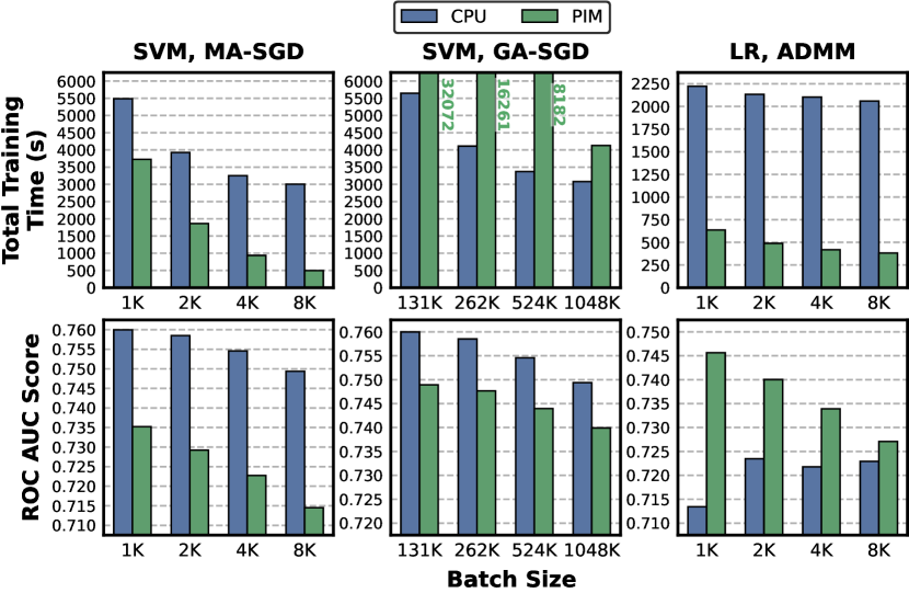
Figure 11: Impact on performance for varying batch size in terms of total training time for $10$ global epochs and ROC AUC score reached in the last global epoch.

Obsv. 18. As batch size decreases, PIM and the CPU architecture exhibit performance degradation for MA-SGD. For ADMM, decreasing the batch size only slightly diminishes performance for both PIM and the CPU architecture.

When batch size decreases from $8$K to $1$K, the total training time of SVM MA-SGD on PIM/CPU architecture increases by $7.53$x/$1.83$x from $494.98$s/$3004.8$s to $3725.71$s/$5488.46$s. This observation is attributed to larger batch sizes, which reduce the total number of communications. The speedup on PIM is higher because, on PIM, we consider more workers leading to more communication, and as discussed previously, communication between PIM and the parameter server is very expensive.

Obsv. 19. Both PIM and the CPU architecture benefit from larger batch sizes for training high-dimensional sparse models with GA-SGD.

For GA-SGD, for both PIM and the CPU architecture, we observe a significant reduction in total training time as we increase the batch size while jointly the test accuracy only slightly degrades. This coincides with our Obsv. 5.1 for the YFCC100M-HNfc6 dataset.

3 Takeaway 7. When training high-dimensional sparse model PIM has benefits for 1) models that are not sensitive to larger batch sizes, and 2) algorithms that minimize inter-DPU communication.

3

Scaling. In Fig. 12, we compare the total training time (y-axis) for $10$ global epochs (first row of plots), the ROC AUC score reached in the last global epoch (y-axis) (second row of plots) and analyze different optimization algorithms (x-axis). We study the models LR (first column of plots) and SVM (second column of plots). For each subplot, the number of DPUs ($256$, $512$, $1024$, and $2048$) is increased, while the train dataset size is scaled accordingly (weak scaling). For MA-SGD and ADMM, we fix the batch size to $2$K. For GA-SGD, we set the batch size to $262$K.

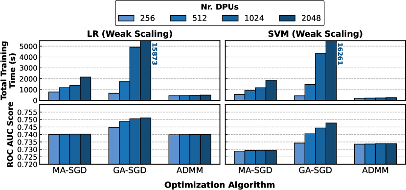
Figure 12: Impact of weak scaling on total training time for $10$ global epochs and ROC AUC score.

Obsv. 20. For high-dimensional sparse models, PIM has good weak scalability with ADMM, but bad weak scalability with MA-SGD and GA-SGD in terms of total training time.

For example, for SVM ADMM/MA-SGD, we observe an increase of total training time by $1.28$x/$3.34$x, while the achieved ROC AUC score changes very slightly as we scale from $256$ to $2048$ DPUs. The speedup gap is higher compared to YFCC100M-HNfc6 as in Obsv. 5.1 because the communication overhead is exacerbated for Criteo’s larger high-dimensional sparse model.

Obsv. 21. Only GA-SGD can profit from a larger training dataset when the number of DPUs is scaled in terms of ROC AUC score.

For SVM GA-SGD, we observe an increase of total training time by $37.82$x, while the achieved ROC AUC score increases by $1.02$x as we scale the number of DPUs from $256$ to $2048$. The observations follow the same line of reasoning as in Obsv. 5.1 for the YFCC100M-HNfc6 dataset.

In Fig. 13, we use the same experiment setting as in Fig. 12, except that, we fix the train dataset size as we scale the number of DPUs (strong scaling).

Figure 13: Impact of strong scaling on total training time for $10$ global epochs and ROC AUC score.

Obsv. 22. For high-dimensional sparse models, PIM has good strong scalability in terms of total training time, but bad in terms of ROC AUC score.

For example, for LR ADMM/MA-SGD, we observe a speedup of $3.85$x/$2.87$x, while the achieved ROC AUC score decreases from $0.74$/$0.74$ to $0.718$/$0.72$, as we scale from $256$ to $2048$ DPUs. In contrast, for LR GA-SGD, we observe an increase in total training time by $3.49$x, while the achieved ROC AUC score changes only very slightly as we scale the number of DPUs from $256$ to $2048$. The slower speedup of ADMM/MA-SGD, and even a slowdown in the case of GA-SGD, compared to YFCC100M-HNfc6, as seen in Obsv. 5.1, is a direct result of the local models communicated in each global epoch for the Criteo dataset being much larger, inducing more expensive communication overhead from the DPUs to the parameter server. The observed reduction of the ROC AUC score follows the same line of reasoning as in the elaborations after Obsv. 5.1 in the case of YFCC100M-HNfc6.

3 Takeaway 8. PIM’s scalability potential for training high-dimensional sparse models is limited by its lack of inter-DPU communication.

3

6 Implications for Hardware Design

Our evaluation in §5 demonstrates that PIM can indeed compete with state-of-the-art processor-centric architectures in various scenarios if algorithms/models are carefully chosen for training of linear models on large-scale datasets. However, to enable ML training on the current PIM hardware infrastructure, several design choices had to be made, such as quantization [64, 65, 66, 67] of the training data/model to avoid floating-point operations and the use of LUTs [62, 21, 63] for hard-to-compute functions.

While future PIM hardware designs should address the design choices mentioned earlier, we believe that the lack of inter-DPU communication in the current PIM design is fundamental because it restricts the set of feasible algorithms to centralized parallel optimization algorithms for PIM. We have shown in our evaluation that ML training can be significantly accelerated for communication-efficient algorithms but also demonstrate that ML training workloads do not scale with the number of DPUs, as one might initially assume. Over the past years, several works have studied decentralized parallel optimization algorithms [74, 75, 76] and their potential advantage over centralized algorithms. It has been theoretically shown that decentralized parallel SGD can achieve the same convergence rate as centralized parallel SGD and is much more robust toward scaling the total number of nodes [75].

Therefore, we believe that inter-DPU communication is key to enable decentralized optimization algorithms in future PIM hardware. Due to the high complexity of the design space, including algorithms, models, training, distributed system topology, and hardware design, we think that a shift towards an algorithm-hardware codesign perspective is necessary in the context of ML training using PIM. With this work, we hope to spark a discussion bridging the gap between the ML and Computer Architecture community to leverage the full potential of ML training workloads using PIM.

7 Related Work

To our knowledge, this is the first paper to implement and rigorously evaluate distributed optimization algorithms commonly used for many data-intensive ML training workloads on a real-world PIM system. In this section, we describe other related works on UPMEM’s PIM system, PIM for ML training and inference, and distributed algorithms.

UPMEM PIM system. There are several prior works on characterization [9, 10, 77] and overview of the architecture [28, 78, 79] of UPMEM’s PIM system. Many prior works explore a variety of algorithms and applications on UPMEM’s PIM system, such as compiler & programming model [43, 80], libraries [62, 29], simulation framework [31, 81], bioinformatics [82, 83, 84, 85], security [86, 87], analytics & databases [88, 89, 90, 91, 92], and ML training/inference [21, 22, 30, 93, 94, 95, 96]. None of the prior works examine the distributed optimization algorithms commonly used for many data-intensive ML training workloads on UPMEM’s PIM system, which this paper implements and rigorously evaluates.

PIM for ML training and inference. There are several works on PIM acceleration for ML training [32, 33, 34, 35, 36, 37]. However, none of these prior works provide a comprehensive evaluation on real-world general-purpose PIM architectures. Another body of works [97, 12, 98, 99, 100, 101, 102, 103, 104, 105, 106, 107, 108, 109, 23, 25, 24, 26, 110] focuses on accelerating inference using PIM.

Distributed algorithms. Other research topics focus on algorithmically alleviating the communication overhead of centralized distributed optimization algorithms since the parameter server has been identified to be the key bottleneck in distributed learning [111, 112, 113, 114]. Other lines of work present decentralized optimization algorithms to minimize communication among many nodes [74, 75, 76].

8 Conclusion

We evaluate and train ML models on large-scale datasets with centralized parallel optimization algorithms on a real-world PIM architecture. We show the importance of carefully choosing the distributed optimization algorithm that fits PIM and analyze tradeoffs. We demonstrate that commercial general-purpose PIM systems can be a viable alternative for many ML training workloads on large-scale datasets to processor-centric architectures. Our results demonstrate the necessity of adapting PIM architectures to enable inter-DPU communication to overcome scalability challenges for many ML training workloads and discuss decentralized parallel SGD optimization algorithms as a potential solution.

References

- [1] S. P. Boyd and L. Vandenberghe, Convex Optimization. Cambridge university press, 2004.
- [2] S. U. Stich, J.-B. Cordonnier, and M. Jaggi, “Sparsified SGD with Memory,” Advances in Neural Information Processing Systems, vol. 31, 2018.
- [3] L. Bottou, “Large-Scale Machine Learning with Stochastic Gradient Descent,” in Proceedings of COMPSTAT’2010: 19th International Conference on Computational StatisticsParis France, August 22-27, 2010 Keynote, Invited and Contributed Papers. Springer, 2010.
- [4] J. Jiang, S. Gan, Y. Liu, F. Wang, G. Alonso, A. Klimovic, A. Singla, W. Wu, and C. Zhang, “Towards Demystifying Serverless Machine Learning Training,” in Proceedings of the 2021 International Conference on Management of Data, 2021.
- [5] P. Villalobos, J. Sevilla, L. Heim, T. Besiroglu, M. Hobbhahn, and A. Ho, “Will we run out of data? An analysis of the limits of scaling datasets in Machine Learning,” arXiv preprint arXiv:2211.04325, 2022.
- [6] M. Wang, W. Fu, X. He, S. Hao, and X. Wu, “A Survey on Large-Scale Machine Learning,” IEEE Transactions on Knowledge and Data Engineering, vol. 34, 2020.
- [7] C. Dünner, T. Parnell, D. Sarigiannis, N. Ioannou, A. Anghel, G. Ravi, M. Kandasamy, and H. Pozidis, “Snap ML: A Hierarchical Framework for Machine Learning,” Advances in Neural Information Processing Systems, vol. 31, 2018.
- [8] B. Cottier, “Trends in the dollar training cost of machine learning systems,” 2023, accessed: 2024-02-25. [Online]. Available: https://epochai.org/blog/trends-in-the-dollar-training-cost-of-machine-learning-systems
- [9] J. Gómez-Luna, I. E. Hajj, I. Fernandez, C. Giannoula, G. F. Oliveira, and O. Mutlu, “Benchmarking a New Paradigm: An Experimental Analysis of a Real Processing-in-Memory Architecture,” arXiv preprint arXiv:2105.03814, 2021.
- [10] J. Gómez-Luna, I. El Hajj, I. Fernandez, C. Giannoula, G. F. Oliveira, and O. Mutlu, “Benchmarking Memory-Centric Computing Systems: Analysis of Real Processing-In-Memory Hardware,” in 2021 12th International Green and Sustainable Computing Conference (IGSC). IEEE, 2021.
- [11] A. Ivanov, N. Dryden, T. Ben-Nun, S. Li, and T. Hoefler, “Data Movement is All You Need: A Case Study on Optimizing Transformers,” in MLSys, 2021.
- [12] A. Boroumand, S. Ghose, Y. Kim, R. Ausavarungnirun, E. Shiu, R. Thakur, D. Kim, A. Kuusela, A. Knies, P. Ranganathan et al., “Google Workloads for Consumer Devices: Mitigating Data Movement Bottlenecks,” in ASPLOS, 2018.
- [13] O. Mutlu, “Intelligent Architectures for Intelligent Computing Systems,” DATE — Invited Talk, 2021.
- [14] O. Mutlu, S. Ghose, J. Gómez-Luna, and R. Ausavarungnirun, “Processing data where it makes sense: Enabling in-memory computation,” Microprocessors and Microsystems, vol. 67, 2019.
- [15] O. Mutlu, S. Ghose, J. Gómez-Luna, and R. Ausavarungnirun, “A Modern Primer on Processing in Memory,” in Emerging Computing: From Devices to Systems: Looking Beyond Moore and Von Neumann. Springer, 2022, pp. 171–243.
- [16] S. Ghose, A. Boroumand, J. S. Kim, J. Gómez-Luna, and O. Mutlu, “Processing-in-memory: A workload-driven perspective,” IBM Journal of Research and Development, vol. 63, 2019.
- [17] V. Seshadri and O. Mutlu, “In-DRAM Bulk Bitwise Execution Engine,” arXiv preprint arXiv:1905.09822, 2019.
- [18] O. Mutlu, S. Ghose, J. Gómez-Luna, and R. Ausavarungnirun, “Enabling Practical Processing in and near Memory for Data-Intensive Computing,” in Proceedings of the 56th Annual Design Automation Conference 2019, 2019.
- [19] W. H. Kautz, “Cellular Logic-in-Memory Arrays,” IEEE Transactions on Computers, vol. 100, 1969.
- [20] H. S. Stone, “A Logic-in-Memory Computer,” IEEE Transactions on Computers, vol. 100, 1970.
- [21] J. Gómez-Luna, Y. Guo, S. Brocard, J. Legriel, R. Cimadomo, G. F. Oliveira, G. Singh, and O. Mutlu, “An Experimental Evaluation of Machine Learning Training on a Real Processing-in-Memory System,” arXiv preprint arXiv:2207.07886, 2022.
- [22] J. Gómez-Luna, Y. Guo, S. Brocard, J. Legriel, R. Cimadomo, G. F. Oliveira, G. Singh, and O. Mutlu, “Evaluating Machine Learning Workloads on Memory-Centric Computing Systems,” in 2023 IEEE International Symposium on Performance Analysis of Systems and Software (ISPASS). IEEE, 2023.
- [23] Y.-C. Kwon, S. H. Lee, J. Lee, S.-H. Kwon, J. M. Ryu, J.-P. Son, O. Seongil, H.-S. Yu, H. Lee, S. Y. Kim et al., “25.4 A 20nm 6GB Function-In-Memory DRAM, Based on HBM2 with a 1.2TFLOPS Programmable Computing Unit Using Bank-Level Parallelism, for Machine Learning Applications,” in 2021 IEEE International Solid-State Circuits Conference (ISSCC), vol. 64. IEEE, 2021.
- [24] L. Ke, X. Zhang, J. So, J.-G. Lee, S.-H. Kang, S. Lee, S. Han, Y. Cho, J. H. Kim, Y. Kwon et al., “Near-Memory Processing in Action: Accelerating Personalized Recommendation With AXDIMM,” IEEE Micro, 2021.
- [25] S. Lee, S.-h. Kang, J. Lee, H. Kim, E. Lee, S. Seo, H. Yoon, S. Lee, K. Lim, H. Shin et al., “Hardware Architecture and Software Stack for PIM Based on Commercial DRAM Technology : Industrial Product,” in ISCA, 2021.
- [26] S. Lee, K. Kim, S. Oh, J. Park, G. Hong, D. Ka, K. Hwang, J. Park, K. Kang, J. Kim et al., “A 1ynm 1.25V 8Gb, 16Gb/s/pin GDDR6-based Accelerator-in-Memory supporting 1TFLOPS MAC Operation and Various Activation Functions for Deep-Learning Applications,” in ISSCC, 2022.
- [27] A. A. Khan, J. P. C. De Lima, H. Farzaneh, and J. Castrillon, “The Landscape of Compute-near-memory and Compute-in-memory: A Research and Commercial Overview,” arXiv preprint arXiv:2401.14428, 2024.
- [28] F. Devaux, “The true Processing in Memory accelerator,” in 2019 IEEE Hot Chips 31 Symposium (HCS). IEEE Computer Society, 2019.
- [29] C. Giannoula, I. Fernandez, J. G. Luna, N. Koziris, G. Goumas, and O. Mutlu, “SparseP: Towards Efficient Sparse Matrix Vector Multiplication on Real Processing-In-Memory Architectures,” Proceedings of the ACM on Measurement and Analysis of Computing Systems, vol. 6, 2022.
- [30] C. Giannoula, P. Yang, I. F. Vega, J. Yang, Y. X. Li, J. G. Luna, M. Sadrosadati, O. Mutlu, and G. Pekhimenko, “Accelerating Graph Neural Networks on Real Processing-In-Memory Systems,” arXiv preprint arXiv:2402.16731, 2024.
- [31] B. Hyun, T. Kim, D. Lee, and M. Rhu, “Pathfinding Future PIM Architectures by Demystifying a Commercial PIM Technology,” arXiv preprint arXiv:2308.00846, 2023.
- [32] M. Gao, G. Ayers, and C. Kozyrakis, “Practical Near-Data Processing for In-Memory Analytics Frameworks,” in 2015 International Conference on Parallel Architecture and Compilation (PACT). IEEE, 2015.
- [33] H. Falahati, P. Lotfi-Kamran, M. Sadrosadati, and H. Sarbazi-Azad, “ORIGAMI: A Heterogeneous Split Architecture for In-Memory Acceleration of Learning,” arXiv preprint arXiv:1812.11473, 2018.
- [34] J. Vieira, N. Roma, P. Tomás, P. Ienne, and G. Falcao, “Exploiting Compute Caches for Memory Bound Vector Operations,” in 2018 30th International Symposium on Computer Architecture and High Performance Computing (SBAC-PAD). IEEE, 2018.
- [35] Z. Sun, G. Pedretti, A. Bricalli, and D. Ielmini, “One-step regression and classification with cross-point resistive memory arrays,” Science advances, vol. 6, 2020.
- [36] C. F. Shelor and K. M. Kavi, “Reconfigurable dataflow graphs for processing-in-memory,” in Proceedings of the 20th International Conference on Distributed Computing and Networking, 2019.
- [37] J. Saikia, S. Yin, Z. Jiang, M. Seok, and J.-s. Seo, “K-Nearest Neighbor Hardware Accelerator Using In-Memory Computing SRAM,” in 2019 IEEE/ACM International Symposium on Low Power Electronics and Design (ISLPED). IEEE, 2019.
- [38] B. T. Polyak, “Introduction to optimization,” 1987.
- [39] P. Zhou, J. Feng, C. Ma, C. Xiong, S. C. H. Hoi et al., “Towards Theoretically Understanding Why Sgd Generalizes Better Than Adam in Deep Learning,” Advances in Neural Information Processing Systems, vol. 33, 2020.
- [40] UPMEM. (2024) UPMEM website. https://www.upmem.com. Accessed: 2024-02-19.
- [41] UPMEM, UPMEM Processing In-Memory (PIM) Tech paper, 2022.
- [42] UPMEM, Product Sheet UPMEM, 2022.
- [43] J. Chen, J. Gómez-Luna, I. El Hajj, Y. Guo, and O. Mutlu, “SimplePIM: A Software Framework for Productive and Efficient Processing-in-Memory,” in 2023 32nd International Conference on Parallel Architectures and Compilation Techniques (PACT). IEEE, 2023.
- [44] M. Zinkevich, M. Weimer, L. Li, and A. Smola, “Parallelized Stochastic Gradient Descent,” Advances in neural information processing systems, vol. 23, 2010.
- [45] R. McDonald, K. Hall, and G. Mann, “Distributed Training Strategies for the Structured Perceptron,” in Human language technologies: The 2010 annual conference of the North American chapter of the association for computational linguistics, 2010.
- [46] O. Dekel, R. Gilad-Bachrach, O. Shamir, and L. Xiao, “Optimal Distributed Online Prediction Using Mini-Batches,” Journal of Machine Learning Research, vol. 13, 2012.
- [47] M. Li, D. G. Andersen, A. J. Smola, and K. Yu, “Communication Efficient Distributed Machine Learning with the Parameter Server,” Advances in Neural Information Processing Systems, vol. 27, 2014.
- [48] S. Boyd, N. Parikh, E. Chu, B. Peleato, J. Eckstein et al., “Distributed Optimization and Statistical Learning via the Alternating Direction Method of Multipliers,” Foundations and Trends® in Machine learning, vol. 3, 2011.
- [49] G. Amato, F. Falchi, C. Gennaro, and F. Rabitti, “YFCC100M-HNfc6: A Large-scale Deep Features Benchmark for Similarity Search,” in SISAP, 2016.
- [50] Criteo AI Lab, “Criteo 1TB Click Logs Dataset,” https://ailab.criteo.com/download-criteo-1tb-click-logs-dataset/, 2014, accessed: 2024-01-31.
- [51] I. Goodfellow, Y. Bengio, and A. Courville, Deep Learning. The MIT Press, 2016.
- [52] J. Zhang, C. De Sa, I. Mitliagkas, and C. Ré, “Parallel SGD: When does averaging help?” arXiv preprint arXiv:1606.07365, 2016.
- [53] H. Yu, S. Yang, and S. Zhu, “Parallel Restarted SGD with Faster Convergence and Less Communication: Demystifying Why Model Averaging Works for Deep Learning,” in Proceedings of the AAAI Conference on Artificial Intelligence, vol. 33, no. 01, 2019.
- [54] UPMEM, “UPMEM SDK, version 2023.2.0,” https://sdk.upmem.com/2023.2.0/, 2023, accessed: 2023-08-28.
- [55] X. Xie, W. Tan, L. L. Fong, and Y. Liang, “CuMF_SGD: Parallelized Stochastic Gradient Descent for Matrix Factorization on GPUs,” in Proceedings of the 26th International Symposium on High-Performance Parallel and Distributed Computing, 2017.
- [56] C. De Sa, M. Feldman, C. Ré, and K. Olukotun, “Understanding and Optimizing Asynchronous Low-Precision Stochastic Gradient Descent,” in Proceedings of the 44th annual international symposium on computer architecture, 2017.
- [57] H. Kim, H. Park, T. Kim, K. Cho, E. Lee, S. Ryu, H.-J. Lee, K. Choi, and J. Lee, “GradPIM: A Practical Processing-in-DRAM Architecture for Gradient Descent,” in 2021 IEEE International Symposium on High-Performance Computer Architecture (HPCA). IEEE, 2021.
- [58] D. Mahajan, J. Park, E. Amaro, H. Sharma, A. Yazdanbakhsh, J. K. Kim, and H. Esmaeilzadeh, “TABLA: A unified template-based framework for accelerating statistical machine learning,” in 2016 IEEE International Symposium on High Performance Computer Architecture (HPCA). IEEE, 2016.
- [59] J. Wang, W. Wang, and N. Srebro, “Memory and Communication Efficient Distributed Stochastic Optimization with Minibatch Prox,” in Conference on Learning Theory. PMLR, 2017.
- [60] W.-S. Chin, Y. Zhuang, Y.-C. Juan, and C.-J. Lin, “A Fast Parallel Stochastic Gradient Method for Matrix Factorization in Shared Memory Systems,” ACM Transactions on Intelligent Systems and Technology (TIST), vol. 6, 2015.
- [61] W.-S. Chin, Y. Zhuang, Y.-C. Juan, and C.-J. Lin, “A Learning-Rate Schedule for Stochastic Gradient Methods to Matrix Factorization,” in Advances in Knowledge Discovery and Data Mining: 19th Pacific-Asia Conference, PAKDD 2015, Ho Chi Minh City, Vietnam, May 19-22, 2015, Proceedings, Part I 19. Springer, 2015.
- [62] M. Item, J. Gómez-Luna, G. F. Oliveira, M. Sadrosadati, Y. Guo, and O. Mutlu, “TransPimLib: Efficient Transcendental Functions for Processing-in-Memory Systems,” in ISPASS, 2023.
- [63] J. D. Ferreira, G. Falcao, J. Gómez-Luna, M. Alser, L. Orosa, M. Sadrosadati, J. S. Kim, G. F. Oliveira, T. Shahroodi, A. Nori et al., “pLUTo: Enabling Massively Parallel Computation in DRAM via Lookup Tables,” in 2022 55th IEEE/ACM International Symposium on Microarchitecture (MICRO). IEEE, 2022.
- [64] Z. Wang, K. Kara, H. Zhang, G. Alonso, O. Mutlu, and C. Zhang, “Accelerating generalized linear models with MLWeaving: a one-size-fits-all system for any-precision learning,” Proceedings of the VLDB Endowment, vol. 12, 2019.
- [65] E. Chung, J. Fowers, K. Ovtcharov, M. Papamichael, A. Caulfield, T. Massengill, M. Liu, D. Lo, S. Alkalay, M. Haselman et al., “Serving DNNs in Real Time at Datacenter Scale with Project Brainwave,” iEEE Micro, vol. 38, 2018.
- [66] S. Han, H. Mao, and W. J. Dally, “Deep Compression: Compressing Deep Neural Networks with Pruning, Trained Quantization and Huffman Coding,” arXiv preprint arXiv:1510.00149, 2015.
- [67] Y. Umuroglu, N. J. Fraser, G. Gambardella, M. Blott, P. Leong, M. Jahre, and K. Vissers, “FINN: A Framework for Fast, Scalable Binarized Neural Network Inference,” in Proceedings of the 2017 ACM/SIGDA international symposium on field-programmable gate arrays, 2017.
- [68] B. Thomee, D. A. Shamma, G. Friedland, B. Elizalde, K. Ni, D. Poland, D. Borth, and L.-J. Li, “YFCC100M: The New Data in Multimedia Research,” Communications of the ACM, 2016.
- [69] R.-E. Fan, “LIBSVM Data: A Collection of Benchmarks for Support Vector Machine Research,” https://www.csie.ntu.edu.tw/~cjlin/libsvmtools/datasets/, accessed: 2023-01-31.
- [70] S. Geman, E. Bienenstock, and R. Doursat, “Neural Networks and the Bias/Variance Dilemma,” Neural computation, vol. 4, 1992.
- [71] F. Zhou and G. Cong, “On the convergence properties of a -step averaging stochastic gradient descent algorithm for nonconvex optimization,” arXiv preprint arXiv:1708.01012, 2017.
- [72] Z. Zhang, J. Jiang, W. Wu, C. Zhang, L. Yu, and B. Cui, “MLlib*: Fast Training of GLMs Using Spark MLlib,” in 2019 IEEE 35th International Conference on Data Engineering (ICDE). IEEE Computer Society, 2019.
- [73] M. Wortsman, S. Gururangan, S. Li, A. Farhadi, L. Schmidt, M. Rabbat, and A. S. Morcos, “Lo-fi: Distributed Fine-tuning Without Communication,” arXiv:2210.11948, 2022.
- [74] J. Liu, C. Zhang et al., “Distributed Learning Systems with First-Order Methods,” Foundations and Trends® in Databases, vol. 9, 2020.
- [75] X. Lian, C. Zhang, H. Zhang, C.-J. Hsieh, W. Zhang, and J. Liu, “Can Decentralized Algorithms Outperform Centralized Algorithms? A Case Study for Decentralized Parallel Stochastic Gradient Descent,” Advances in neural information processing systems, vol. 30, 2017.
- [76] G. Lan, S. Lee, and Y. Zhou, “Communication-efficient algorithms for decentralized and stochastic optimization,” Mathematical Programming, vol. 180, 2020.
- [77] J. Nider, C. Mustard, A. Zoltan, J. Ramsden, L. Liu, J. Grossbard, M. Dashti, R. Jodin, A. Ghiti, J. Chauzi et al., “A case study of Processing-in-Memory in off-the-Shelf systems,” in 2021 USENIX Annual Technical Conference (USENIX ATC 21), 2021.
- [78] B. Peccerillo, M. Mannino, A. Mondelli, and S. Bartolini, “A survey on hardware accelerators: Taxonomy, trends, challenges, and perspectives,” Journal of Systems Architecture, vol. 129, 2022.
- [79] UPMEM, “UPMEM PIM platform for Data-Intensive Applications,” in ABUMPIMP. Symposium as part of Euro-Par, 2023, accessed: 2024-04-05. [Online]. Available: {https://www.youtube.com/watch?v=xsTp6raY6fE}
- [80] A. A. Khan, H. Farzaneh, K. F. Friebel, C. Fournier, L. Chelini, and J. Castrillon, “CINM (Cinnamon): A Compilation Infrastructure for Heterogeneous Compute In-Memory and Compute Near-Memory Paradigms,” arXiv preprint arXiv:2301.07486, 2022.
- [81] B. Hyun, T. Kim, D. Lee, and M. Rhu, “Pathfinding Future PIM Architectures by Demystifying a Commercial PIM Technology,” in 2024 IEEE International Symposium on High-Performance Computer Architecture (HPCA). IEEE, 2024.
- [82] L.-C. Chen, C.-C. Ho, and Y.-H. Chang, “UpPipe: A Novel Pipeline Management on In-Memory Processors for RNA-seq Quantification,” in 2023 60th ACM/IEEE Design Automation Conference (DAC). IEEE, 2023.
- [83] S. Diab, A. Nassereldine, M. Alser, J. Gómez Luna, O. Mutlu, and I. El Hajj, “A framework for high-throughput sequence alignment using real processing-in-memory systems,” Bioinformatics, vol. 39, 2023.
- [84] D. Lavenier, R. Cimadomo, and R. Jodin, “Variant Calling Parallelization on Processor-in-Memory Architecture,” in 2020 IEEE International Conference on Bioinformatics and Biomedicine (BIBM). IEEE, 2020.
- [85] D. Lavenier, C. Deltel, D. Furodet, and J.-F. Roy, “BLAST on UPMEM,” Ph.D. dissertation, INRIA Rennes-Bretagne Atlantique, 2016.
- [86] H. Gupta, M. Kabra, J. Gómez-Luna, K. Kanellopoulos, and O. Mutlu, “Evaluating Homomorphic Operations on a Real-World Processing-In-Memory System,” in 2023 IEEE International Symposium on Workload Characterization (IISWC). IEEE, 2023.
- [87] G. Jonatan, H. Cho, H. Son, X. Wu, N. Livesay, E. Mora, K. Shivdikar, J. L. Abellán, A. Joshi, D. Kaeli et al., “Scalability Limitations of Processing-in-Memory using Real System Evaluations,” Proceedings of the ACM on Measurement and Analysis of Computing Systems, vol. 8, 2024.
- [88] A. Bernhardt, A. Koch, and I. Petrov, “pimDB: From Main-Memory DBMS to Processing-In-Memory DBMS-Engines on Intelligent Memories,” in Proceedings of the 19th International Workshop on Data Management on New Hardware, 2023.
- [89] C. Lim, S. Lee, J. Choi, J. Lee, S. Park, H. Kim, J. Lee, and Y. Kim, “Design and Analysis of a Processing-in-DIMM Join Algorithm: A Case Study with UPMEM DIMMs,” Proceedings of the ACM on Management of Data, vol. 1, 2023.
- [90] A. Baumstark, M. A. Jibril, and K.-U. Sattler, “Adaptive Query Compilation with Processing-in-Memory,” in 2023 IEEE 39th International Conference on Data Engineering Workshops (ICDEW). IEEE, 2023.
- [91] A. Baumstark, M. A. Jibril, and K.-U. Sattler, “Accelerating Large Table Scan Using Processing-In-Memory Technology,” Datenbank-Spektrum, vol. 23, 2023.
- [92] H. Kang, Y. Zhao, G. E. Blelloch, L. Dhulipala, Y. Gu, C. McGuffey, and P. B. Gibbons, “PIM-trie: A Skew-resistant Trie for Processing-in-Memory,” in Proceedings of the 35th ACM Symposium on Parallelism in Algorithms and Architectures, 2023.
- [93] P. Das, P. R. Sutradhar, M. Indovina, S. M. P. Dinakarrao, and A. Ganguly, “Implementation and Evaluation of Deep Neural Networks in Commercially Available Processing in Memory Hardware,” in 2022 IEEE 35th International System-on-Chip Conference (SOCC). IEEE, 2022.
- [94] N. Zarif, “Offloading embedding lookups to processing-in-memory for deep learning recommender models,” Master’s thesis, University of British Columbia, 2023, accessed: 2024-04-05. [Online]. Available: https://open.library.ubc.ca/collections/ubctheses/24/items/1.0435518
- [95] S. Y. Kim, J. Lee, Y. Paik, C. H. Kim, W. J. Lee, and S. W. Kim, “Optimal Model Partitioning with Low-Overhead Profiling on the PIM-based Platform for Deep Learning Inference,” ACM Transactions on Design Automation of Electronic Systems, vol. 29, 2024.
- [96] Y. Wu, Z. Wang, and W. D. Lu, “PIM-GPT: A Hybrid Process-in-Memory Accelerator for Autoregressive Transformers,” arXiv preprint arXiv:2310.09385, 2023.
- [97] Q. Deng, L. Jiang, Y. Zhang, M. Zhang, and J. Yang, “DrAcc: A DRAM based accelerator for accurate CNN inference,” in Proceedings of the 55th annual design automation conference, 2018.
- [98] M. Gao, J. Pu, X. Yang, M. Horowitz, and C. Kozyrakis, “TETRIS: Scalable and Efficient Neural Network Acceleration with 3D Memory,” in Proceedings of the Twenty-Second International Conference on Architectural Support for Programming Languages and Operating Systems, 2017.
- [99] A. Boroumand, S. Ghose, B. Akin, R. Narayanaswami, G. F. Oliveira, X. Ma, E. Shiu, and O. Mutlu, “Google Neural Network Models for Edge Devices: Analyzing and Mitigating Machine Learning Inference Bottlenecks,” in 2021 30th International Conference on Parallel Architectures and Compilation Techniques (PACT). IEEE, 2021.
- [100] S. Cho, H. Choi, E. Park, H. Shin, and S. Yoo, “McDRAM v2: In-Dynamic Random Access Memory Systolic Array Accelerator to Address the Large Model Problem in Deep Neural Networks on the Edge,” IEEE Access, vol. 8, 2020.
- [101] H. Shin, D. Kim, E. Park, S. Park, Y. Park, and S. Yoo, “McDRAM: Low Latency and Energy-Efficient Matrix Computations in DRAM,” IEEE Transactions on Computer-Aided Design of Integrated Circuits and Systems, vol. 37, 2018.
- [102] E. Azarkhish, D. Rossi, I. Loi, and L. Benini, “Neurostream: Scalable and Energy Efficient Deep Learning with Smart Memory Cubes,” IEEE Transactions on Parallel and Distributed Systems, vol. 29, 2017.
- [103] Y. Kwon, Y. Lee, and M. Rhu, “TensorDIMM: A Practical Near-Memory Processing Architecture for Embeddings and Tensor Operations in Deep Learning,” in Proceedings of the 52nd Annual IEEE/ACM International Symposium on Microarchitecture, 2019.
- [104] L. Ke, U. Gupta, B. Y. Cho, D. Brooks, V. Chandra, U. Diril, A. Firoozshahian, K. Hazelwood, B. Jia, H.-H. S. Lee et al., “RecNMP: Accelerating Personalized Recommendation with Near-Memory Processing,” in 2020 ACM/IEEE 47th Annual International Symposium on Computer Architecture (ISCA). IEEE, 2020.
- [105] A. S. Cordeiro, S. R. dos Santos, F. B. Moreira, P. C. Santos, L. Carro, and M. A. Alves, “Machine Learning Migration for Efficient Near-Data Processing,” in 2021 29th Euromicro International Conference on Parallel, Distributed and Network-Based Processing (PDP). IEEE, 2021.
- [106] Y. S. Lee and T. H. Han, “Task Parallelism-Aware Deep Neural Network Scheduling on Multiple Hybrid Memory Cube-Based Processing-in-Memory,” IEEE Access, vol. 9, 2021.
- [107] N. Park, S. Ryu, J. Kung, and J.-J. Kim, “High-throughput Near-Memory Processing on CNNs with 3D HBM-like Memory,” ACM Transactions on Design Automation of Electronic Systems (TODAES), vol. 26, 2021.
- [108] J. Park, B. Kim, S. Yun, E. Lee, M. Rhu, and J. H. Ahn, “TRiM: Enhancing Processor-Memory Interfaces with Scalable Tensor Reduction in Memory,” in MICRO-54: 54th Annual IEEE/ACM International Symposium on Microarchitecture, 2021.
- [109] B. Kim, J. Chung, E. Lee, W. Jung, S. Lee, J. Choi, J. Park, M. Wi, S. Lee, and J. H. Ahn, “MViD: Sparse Matrix-Vector Multiplication in Mobile DRAM for Accelerating Recurrent Neural Networks,” IEEE Transactions on Computers, vol. 69, 2020.
- [110] D. Niu, S. Li, Y. Wang, W. Han, Z. Zhang, Y. Guan, T. Guan, F. Sun, F. Xue, L. Duan et al., “184QPS/W 64Mb/mm 2 3D logic-to-DRAM hybrid bonding with process-near-memory engine for recommendation system,” in 2022 IEEE International Solid-State Circuits Conference (ISSCC), vol. 65. IEEE, 2022.
- [111] J. Wang, Y. Lu, B. Yuan, B. Chen, P. Liang, C. De Sa, C. Re, and C. Zhang, “CocktailSGD: Fine-tuning Foundation Models over 500Mbps Networks,” in International Conference on Machine Learning. PMLR, 2023.
- [112] H. Xu, C.-Y. Ho, A. M. Abdelmoniem, A. Dutta, E. H. Bergou, K. Karatsenidis, M. Canini, and P. Kalnis, “Compressed communication for distributed deep learning: Survey and quantitative evaluation,” Tech. Rep., 2020.
- [113] D. Alistarh, D. Grubic, J. Li, R. Tomioka, and M. Vojnovic, “QSGD: Communication-efficient SGD via gradient quantization and encoding,” Advances in neural information processing systems, vol. 30, 2017.
- [114] N. Ström, “Scalable distributed DNN training using commodity GPU cloud computing,” Sixteenth annual conference of the international speech communication association, 2015.