On noise in swap ASAP repeater chains:
exact analytics, distributions and tight approximations

Abstract

Losses are one of the main bottlenecks for the distribution of entanglement in quantum networks, which can be overcome by the implementation of quantum repeaters. The most basic form of a quantum repeater chain is the swap ASAP repeater chain. In such a repeater chain, elementary links are probabilistically generated and deterministically swapped as soon as two adjacent links have been generated. As each entangled state is waiting to be swapped, decoherence is experienced, turning the fidelity of the entangled state between the end nodes of the chain into a random variable. Fully characterizing the (average) fidelity as the repeater chain grows is still an open problem. Here, we analytically investigate the case of equally-spaced repeaters, where we find exact analytic formulae for all moments of the fidelity up to $25$ segments. We obtain these formulae by providing a general solution in terms of a generating function; a function whose $n$’th term in its Maclaurin series yields the moments of the fidelity for $n$ segments. We generalize this approaches as well to a global cut-off policy — a method for increasing fidelity at the cost of longer entanglement delivery times — allowing for fast optimization of the cut-off parameter by eliminating the need for Monte Carlo simulation. We furthermore find simple approximations of the average fidelity that are exponentially tight, and, for up to 10 segments, the full distribution of the delivered fidelity. We use this to analytically calculate the secret-key rate when the distributed entanglement is used for quantum-key distribution, both with and without binning methods. In follow-up work we exploit a connection to a model in statistical physics to numerically calculate quantities of interest for the inhomogeneous multipartite case.

separator=,, divider=bar,

I Introduction

Quantum communication allows for benefits inaccessible with classical communication alone, key examples including secure key distribution bennett2020quantum ; ekert1991quantum , secret sharing hillery1999quantum ; markham2008graph and distributed quantum computation cirac1999distributed ; serafini2006distributed . These protocols all rely on end-users sharing entanglement. A quantum internet wehner2018quantum would allow for the distribution of such entanglement over large distances. One way to achieve this distribution is to transmit states over optical fibers; this has the benefit of being able to use pre-existing classical infrastructure rabbie2022designing .

One bottleneck of quantum communication is losses, where the success probability of a single photon arriving end-to-end over a distance $L$ is given by $p=~{}\exp(-\frac{L}{L_{\textrm{att}}})$, $L_{\textrm{att}}\approx 22$ kilometers. A naive amplification of the signal to overcome this (as one does in the classical case) is prohibited by the no-cloning theorem. Fortunately, quantum repeaters briegel1998quantum provide a solution. That is, by splitting the total length into $n$ segments and generating entanglement over the segments, end-to-end entanglement can be created by performing so-called entanglement swaps azuma2022quantum . Assuming that entanglement is swapped as soon as possible (swap ASAP) one can show that the state delivery rate now scales as $\mathcal{O}\left({}^{n}\sqrt{p}\right)$ (where we assume here and in the rest of the paper that the swaps are deterministic). Thus, while the rate still decays exponentially with the distance, the delivery rate increases significantly compared to the case without repeaters.

Although repeaters have the ability to increase the delivery rate, they also introduce additional noise, lowering the quality of the delivered entanglement. There are two contributions to this additional noise rozpkedek2018parameter ; rozpkedek2019near . First, noise arising from imperfections in the devices (such as state preparation); second, noise arising from memory decoherence. Note that the first type of noise is deterministic. In contrast, the second type of noise is random. This is due to the fact that a node needs to wait for a random amount of time until both its incident links are present before a swap can be performed. This random noise causes the fidelity of the end-to-end state to be a random variable.

The trade-off between increasing the rate and the average fidelity complicates understanding what can be done with near-term devices, especially in combination with so-called cut-off policies. A cut-off policy is one that sets a threshold for when to discard the present entanglement. After this discard, the entanglement generation is started anew. Discarding generated entanglement reduces the rate at which entanglement is delivered, but, by a clever choice of a cut-off policy, will mitigate the time spent on distributing end-to-end entanglement with too low a fidelity. A cut-off policy thus allows for a trade-off between the rate and quality of the delivered end-to-end entanglement. Cut-off policies and their trade-offs have been studied, for example, in rozpkedek2018parameter ; rozpkedek2019near ; collins2007multiplexed ; avis2022requirements ; li2020efficient ; khatri2019practical ; santra2018quantum ; davies2023tools ; azuma2021tools ; praxmeyer2013reposition ; kamin2023exact ; shchukin2019waiting ; reiss2023deep ; zang2023entanglement .

However, analytic expressions for the expected fidelity in the presence or absence of cut-off policies have been derived only up to $8$ segments kamin2023exact . Here, we analytically calculate the average fidelity of the delivered state for homogeneous swap ASAP repeater chains up to length $25$. Furthermore, we find closed-form expressions for the probability distribution of the fidelity for up to $10$ segments. While the analytical expressions grow unwieldy very fast, we find a closed-form expression of a so-called generating function — a function whose Maclaurin series coefficients correspond to the average noise parameters. This, in a sense, fully characterizes the average noise for swap ASAP repeater chains of arbitrary lengths. Using tools from analytic combinatorics, we use this generating function to find simple approximations that are provably asymptotically tight, and which in practice are indistinguishable from exact results already for three and more segments. As a caveat, we assume for the exact analytics that the end nodes experience no decoherence, which holds when performing quantum key distribution (QKD) bennett2020quantum (when the states at the end nodes can be measured directly) or can be justified in the case where the end nodes have significantly more resources than the repeater chain, see also kamin2023exact for a similar setup.

We note that a specific type of generating function, the probability generating function, has been used before in the noise analysis for more general quantum repeater protocols, ranging up to $n=8$ segments for a full analysis of all moments of the fidelity kamin2023exact . Our generating function is strictly more powerful, since it captures all probability generating functions at once; its $n$’th term is exactly the probability generating function associated to $n$ segments. This thus provides an explanation for the expressions from kamin2023exact , where the expressions were found through brute-force calculation. By taking appropriate derivatives/expansions of our generating function, we compute an analytical expression of the average fidelity up to 25 segments within seconds, and find an analytical expression for the distribution of the fidelity up to 10 repeater segments.

We also show how most of our tools can be applied to a global cut-off policy. This cut-off policy does not require any communication between the nodes, making it especially relevant for near-term quantum networks.

We show how our tools can be used to 1) understand the effect of adding or removing repeaters for a given distance, 2) derive the distribution of the noise and how it relates to the cut-off threshold, 3) calculate the secret-key rate exactly for up to 10 segments, with and without so-called binning strategies, 4) understand the interaction between decoherence and losses in a manner that is independent of the number of repeaters.

All of our analytical results can be found in the provided Mathematica files mathematicafiles .

We leave most of the technical details to the Appendix, and focus on the general concepts in the main text. We start by making explicit our model in Section II, where we also discuss the global cut-off policy. In Section III we give a general overview of how to calculate exact analytics (with and without a global cut-off). Section IV presents an overview of the derivation of the approximation for the average fidelity, which is based on techniques from analytic combinatorics. For our final result we focus in Section V, not on the average fidelity, but on the associated distribution. We close each of the previous three sections by applying our tools to numerical exploration of repeater chains. We conclude with a discussion in Section VI, where we discuss possible extensions and touch upon follow-up work that extends some of our results numerically to both the inhomogeneous and multipartite setting.

II Swap ASAP repeater model

In this Section we first present the basic setup of a swap ASAP repeater chain in the case of qubit depolarizing noise. We then discuss how our results extend to a large set of other noise models. Afterwards, we discuss the cut-off policy relevant for this work. We note that a similar setup was also investigated in kamin2023exact .

II.1 Model details

The aim of this section is to lay out our model of a swap ASAP repeater chain. A repeater chain consists of $n$ segments, separated by $n-1$ repeater nodes. We order the $n$ segments from left to right by $i=1,\ldots,n$. Swap ASAP means that elementary link generation is attempted in parallel over each segment in a given round. We will assume that rounds are discretized (with duration equal to a single timestep), and label the round in which segment $i$ succeeds by $t_{i}$, where $t_{i}\geq 1$. Link generation succeeds with a uniform probability $p$ across all segments. We assume that link generation is attempted again only after successful end-to-end entanglement generation or after reaching a cut-off condition (see the next subsection). This is not only done to aid in the analysis, but it also prevents congestion and is closer to the capabilities of near-term devices.

As soon as a repeater holds two adjacent links a swap is performed, which we assume to be deterministic. We show an example evolution of a swap ASAP repeater chain in Fig. 1, where $t_{1}=3$, $t_{2}=2$, $t_{3}=4$, $t_{4}=1$ and $t_{5}=2$.

The decoherence experienced in a given run will be determined by the number of rounds each node has to wait until it can swap, along with the quality of the memory. We describe noise in the system with depolarizing noise. That is, our states are of the form $\Lambda\ket{\psi}\bra{\psi}+(1-\Lambda)\frac{\mathbb{I}}{4}$, where $\sqrt{2}\ket{\psi}=\ket{00}+\ket{11}$ and $\Lambda\in[0,1]$. From $\Lambda$, we calculate the fidelity to be $\Lambda+\frac{1-\Lambda}{4}=\frac{3}{4}\Lambda+\frac{1}{4}$. The usage of the parameter $\Lambda$ is convenient — swapping two states with parameters $\Lambda^{\prime}$ and $\Lambda^{\prime\prime}$ gives a new state with parameter $\Lambda^{\prime}\cdot\Lambda^{\prime\prime}$. Furthermore, decoherence over a single time step corresponds to the map $\Lambda\mapsto\lambda\Lambda$ for some $\lambda\in\left[0,1\right]$. Here and in what follows, we focus on $\Lambda$, since it completely characterizes the quantum state, such that other quality indicators (such as fidelity) can be extracted from it.

Let us consider a concrete example. In Fig. 1 the decoherence experienced by the memory in the repeater holding links $2$ and $3$ is equal to $\lambda^{\left|2-4\right|}=\lambda^{2}$, where $\lambda$ is the noise parameter associated with a single round of decoherence. This is the case since after generating link $2$ at time $t=2$, the memory needed to be stored until time $t=4$ before it could be swapped with link 3.

Importantly, we will ignore the noise that the end nodes would have to incur if they had to keep their states stored until all other links have succeeded. This can be justified exactly when QKD is performed (in which case the states at the end nodes can be measured directly), or when the end nodes are assumed to have significantly better equipment or error correction. See kamin2023exact for a treatment that includes this noise.

With knowledge of which swaps were performed and how long certain memories were decohering, it is possible to calculate the noise parameter $\Lambda$ describing the final state. We show in the next section how to calculate the expectation value of the final noise parameter. Finally, from linearity of expectation, we can calculate the average fidelity $\mathds{E}\left[F\right]=\frac{3}{4}\mathds{E}\left[\Lambda\right]+\frac{1}{4}$ from the average $\Lambda$ parameter.

Figure 1: The used model for a swap ASAP repeater chain. In the top figure a) we show the evolution of the present entanglement in the network. At time $t=1$ the fourth link gets created, at time $t=2$ both link 2 and 5 are generated. Since we are considering the swap ASAP model, link 4 and 5 are swapped at this time. At time $t=3$ link 1 is created and swapped with link 2. Finally, at time $t=4$ the third link is created, which is immediately swapped on both sides, leading to end-to-end entanglement. In b) we summarize the total evolution of a single run. The decoherence experienced corresponds to the waiting time between the different links, indicated by dashed lines. The dotted lines correspond to having to wait until all links have been created, which are not relevant when performing tasks such as QKD.

We note that this model also includes noisy state generation. Namely, if $\Lambda$ is the end-to-end noise parameter for the case of perfect state generation, then the average noise parameter with noisy state generation is given by $\Lambda\cdot\prod_{i=1}^{n}\lambda_{\textrm{gen},i}$. Here $\lambda_{\textrm{gen},i}$ are the noise parameters corresponding to the $n$ noisy links, resulting in a constant multiplicative factor to the $\Lambda$ parameter. In what follows however, we will assume that link generation is perfect unless explicitly mentioned.

II.2 Extension to general noise models

Above, we chose the single-qubit depolarizing channel as the noise model. The properties that make this noise model amenable to analysis is the fact that decoherence corresponds to multiplication of the $\lambda$ parameter, and that swapping two states corresponds to multiplication of the $\lambda$ parameters. We derive in Appendix B that if the state is a two-qubit maximally-entangled state, then any qubit Pauli channel $\mathcal{N}$ has these properties. Consequently, the analysis in this work straightforwardly extends to any qubit Pauli noise model. The parameter update is achieved by a change of variables of $\mathcal{N}$: we start out with the usual parameterization of a Pauli channel,

$$\mathcal{N}(\rho)=p_{I}\cdot\rho+p_{X}\cdot X\rho X^{\dagger}+p_{Y}\cdot Y\rho Y^{\dagger}+p_{Z}\cdot Z\rho Z^{\dagger}\ ,$$

where $\{p_{I},p_{X},p_{Y},p_{Z}\}$ is a probability distribution over the Pauli matrices $I,X,Y,Z$ and $\rho$ a single-qubit density matrix. We now re-parameterize $\mathcal{N}=\mathcal{N}_{\vec{\lambda}}$ using four new variables $\vec{\lambda}=(\lambda_{1},\lambda_{2},\lambda_{3},\lambda_{4})$ which we define as

$$\lambda_{1} =p_{I}+p_{X}+p_{Y}+p_{Z}=1,$$

$$\lambda_{2} =p_{I}+p_{X}-p_{Y}-p_{Z}\ ,$$

$$\lambda_{3} =p_{I}-p_{X}+p_{Y}-p_{Z}\ ,$$

$$\lambda_{4} =p_{I}-p_{X}-p_{Y}+p_{Z}\ .$$

To verify that this change of variables satisfies the above criteria, it is straightforward to calculate that first applying $\mathcal{N}_{\vec{\lambda}}$, followed by applying $\mathcal{N}_{\vec{\lambda}^{\prime}}$, is the same as applying $\mathcal{N}_{\left(\lambda_{1}\cdot\lambda_{1}^{\prime},\lambda_{2}\cdot\lambda_{2}^{\prime},\lambda_{3}\cdot\lambda_{3}^{\prime},\lambda_{4}\cdot\lambda_{4}^{\prime}\right)}$. As a simple example, consider dephasing noise (which was also considered in kamin2023exact ), where

$$\mathcal{N}\left(\cdot\right) =p\left(\cdot\right)+\left(1-p\right)Z\left(\cdot\right)Z^{\dagger}$$ (1)

$$=\left(\frac{1+\lambda_{2}}{2}\right)\left(\cdot\right)+\left(\frac{1-\lambda_{2}}{2}\right)Z\left(\cdot\right)Z^{\dagger}\$$ (2)

$$=\mathcal{N}_{\left(1,1-2p,1-2p,1\right)}\left(\cdot\right)\ .$$ (3)

Multiplicativity under swapping is also satisfied for the general qubit Pauli channel. We denote by $\rho(\vec{\lambda})$ the resultant state after $\mathcal{N}_{\vec{\lambda}}$ has acted on one of the qubits of a maximally entangled state. An entanglement swap on the states $\rho(\vec{\lambda})$ and $\rho(\vec{\lambda}^{\prime})$ then yields the state $\rho(\lambda_{1}\cdot\lambda_{1}^{\prime},\lambda_{2}\cdot\lambda_{2}^{\prime},\lambda_{3}\cdot\lambda_{3}^{\prime},\lambda_{4}\cdot\lambda_{4}^{\prime})$ after correction, independently of the correction that needed to be applied. Since all the $\lambda_{i}$ terms are multiplied pointwisely, all of the analysis that we do in this paper for the $\lambda$ parameter for depolarizing can be directly translated to the individual $\lambda_{i}$ parameters. In Appendix B, we also examine the case where the link between nodes is given by a maximally-entangled states on two qudits, i.e. the more general case where the local Hilbert space has dimension $\geq 2$. Specifically, we show that the multiplicativity properties above hold for $X$-symmetric channels. These are the channels corresponding to a probabilistic application of $d$-dimensional qudit Pauli operators $X^{a}Z^{b}$ (with $a,b\in\{0,1,\dots,d-1\}$), where the probability for $X^{a}Z^{b}$ is equal to the probability for $X^{-a}Z^{b}$. The qubit case follows since any qubit Pauli channel is $X$-symmetric. Our analysis is thus applicable to dephasing (also considered in kamin2023exact ), but also to (biased) depolarizing noise and relevant noise models for GKP qudits, see noh2020fault ; albert2018performance ; shaw2024logical ; noh2018quantum . Our derivation is based on interpreting the composition of qudit Pauli channels as a type of convolution, which allows us to use tools from Fourier theory on finite Abelian groups.

II.3 The global cut-off policy

We will now describe the cut-off policy that we consider in this paper, which we refer to as the global cut-off policy. This policy does not require any of the nodes to communicate information to far away nodes, making this policy particularly appealing for near-term quantum networks. We depict the global cut-off policy visually in Fig. 2. For completeness, we discuss in Appendix A a number of other policies, but which are outside the scope of this paper.

Figure 2: Graphical description of the global cut-off policy. Each of the nodes has agreed on a parameter $T_{c}$. For the global cut-off, a reset is performed when after $T_{c}$ rounds end-to-end entanglement has not been established.

The global cut-off imposes a constraint on how long it may take to establish end-to-end entanglement. That is, starting from a chain with no entanglement present, a timer is initialized to $0$ and increases by one after every elementary link generation attempt. Then, the ordinary swap ASAP protocol is followed. There are two things that can happen. If end-to-end entanglement is established before the timer reaches $T_{c}$, the timer is reset and the swap ASAP protocol is performed once again. If, however, the timer reaches $T_{c}$ rounds (i.e. the cut-off is reached), the present entanglement is thrown away and the swap ASAP protocol starts anew.

Fig. 2 shows an example of the global cut-off policy. In this case, the third link did not succeed before the timer $T_{c}=3$, and the entanglement will be discarded.

III Recursion relation for the swap ASAP repeater model

With the considered model of a swap ASAP repeater chain in hand, we can start to analyze the average end-to-end fidelity.

In subsection III.1 we deal first with the case of no cut-off policy. In subsection III.1.1 we sketch how to generalize the approach of the previous section to a global cut-off. We furthermore also discuss why a similar approach fails for the local cut-off policy, and how to calculate the higher-order moments of $\Lambda$ (which was also done before in kamin2023exact ). We conclude in subsection III.2 by applying our results to parameter exploration for repeaters.

III.1 Analytics without a cut-off policy

First, we need to calculate the probability of observing a specific instance. An instance is characterized by a sequence $\overline{t}=\left(t_{1},t_{2},\ldots,t_{n}\right)$, where the $t_{i}\geq 1$ are integers indicating the round in which link $i$ succeeded, see Section II. A single link $i$ succeeds in round $t_{i}$ with probability $p\left(1-p\right)^{t_{i}-1}=\left(1-q\right)q^{t_{i}-1}$, where $q\equiv 1-p$. A total of $n$ links with associated $\overline{t}=\left(t_{1},t_{2},\ldots,t_{n}\right)$ then occurs with probability

$$\prod_{i=1}^{n}\left(1-q\right)q^{t_{i}-1}$$ (4)

$$= \left(\frac{1-q}{q}\right)^{n}q^{\sum_{i=1}^{n}t_{i}}\ .$$ (5)

Let us now consider the decoherence for a given instance $\overline{t}$. Each node that is not an end node has two neighboring links, which succeed at times $t_{i}$ and $t_{i+1}$. Swapping as soon as possible means that the swap occurs when the latest of the two links got created, i.e. at time $\max(t_{i},t_{i+1})$. The link that got created first was created at time $\min(t_{i},t_{i+1})$. Thus, the corresponding node has to wait $\max(t_{i},t_{i+1})-\min(t_{i},t_{i+1})=\left|t_{i}-t_{i+1}\right|$ time steps, over which the associated memory experiences decoherence.

Since a memory experiences a decay of $\lambda$ for each time step, every node that is not an end node adds a multiplicative factor of $\lambda^{\left|t_{i}-t_{i+1}\right|}$, leading to a total decay parameter of $\Lambda=\lambda^{\sum_{i}^{n-1}\left|t_{i}-t_{i+1}\right|}=\lambda^{K(\overline{t})}$, where $K(\overline{t})\equiv\sum_{i}^{n-1}\left|t_{i}-t_{i+1}\right|$ is the aggregate waiting time. We will also refer to $K$ as the roughness parameter of $\overline{t}$. How about the end nodes? The end nodes have to keep their state stored until end-to-end entanglement has been established. By definition, end-to-end entanglement gets established at $\max(\overline{t})$, so that the first and last node have to store entanglement for $\max(\overline{t})-t_{1}$ and $\max(\overline{t})-t_{n}$ rounds, respectively. This leads to an additional total decoherence parameter of $\lambda^{2\max(\overline{t})-t_{1}-t_{n}}$. The average noise parameter $\mathbb{E}\left[\lambda_{\textrm{end}}\right]$ can then be written as

$$\left(\frac{1-q}{q}\right)^{n}\sum_{\overline{t}}\left(q^{\sum_{i}^{n}t_{i}}\right)\cdot\left(\lambda^{\left(2\max(\overline{t})-t_{1}-t_{n}\right)+\sum_{i}^{n-1}\left|t_{i}-t_{i+1}\right|}\right)\ .$$

As mentioned in the previous section, we will now drop the $\lambda^{2\max(\overline{t})-t_{1}-t_{n}}$ factor.

We are interested in calculating the average noise parameter for $n$ segments, i.e.

$$\mathbb{E}\left[\Lambda_{n}\right]= \left(\frac{1-q}{q}\right)^{n}\sum_{\overline{t}}\left(q^{\sum_{i}^{n}t_{i}}\right)\cdot\left(\lambda^{\sum_{i}^{n-1}\left|t_{i}-t_{i+1}\right|}\right)$$

$$= ~{}\sum_{k=0}^{\infty}P\left(K_{n}=k\right)\lambda^{k}$$

$$= ~{}H_{K_{n}}\left(\lambda\right)$$

$$\equiv ~{}H_{n}\ ,$$ (6)

where $H_{X}\left(z\right)$ is shorthand for the probability generating function of the random variable $X$ and we introduced a subscript to indicate the associated number of segments $n$. It follows that $\mathds{E}\left[\Lambda_{n}\right]$ is equal to the probability generating function of the roughness parameter $K_{n}=\sum_{i=1}^{n-1}\left|t_{i}-t_{i+1}\right|$, first observed in  kamin2023exact . This interpretation is useful for two reasons. First, any method to calculate $\mathds{E}\left[\Lambda_{n}\right]$ (or $\mathds{E}\left[\Lambda_{n}\left(T_{c}\right)\right]$), allows for the determination of any of the higher-order moments $\mathds{E}\left[\left(\Lambda_{n}\right)^{m}\right]$. This can be done by repeating the method but with $\lambda$ replaced by $\lambda^{m}$, since

$$\mathbb{E}\left[\left(\Lambda_{n}\right)^{m}\right]= ~{}\sum_{k=0}^{\infty}P\left(K_{n}=k\right)\left(\lambda^{k}\right)^{m}$$

$$= ~{}\sum_{k=0}^{\infty}P\left(K_{n}=k\right)\left(\lambda^{m}\right)^{k}\ ,$$

noted first in kamin2023exact . Second, it is well known that a probability mass function can be reconstructed from the derivatives of its associated probability generating function; we exploit this idea in Section V. Note that the interpretation of the average noise as the probability generating function of the aggregate waiting time is not specific to swap ASAP repeater chains. This was first noted in kamin2023exact , where they investigated several different methods of entanglement distributions for repeater chains. It would be of interest to see similar tools exploited for further variants of entanglement distribution.

To derive an analytical expression of $\mathds{E}\left[\Lambda_{n}\right]=H_{n}$, it will be convenient to define

$$H_{n}^{t}=\left(\frac{1-q}{q}\right)^{n}\sum_{\mathclap{\begin{subarray}{c}\overline{t}~{}\textrm{s.t.}\\ t_{n}=t\end{subarray}}}\left(q^{\sum_{i=1}^{n}t_{i}}\right)\cdot\left(\lambda^{\sum_{i=1}^{n-1}\left|t_{i}-t_{i+1}\right|}\right)\ .$$ (7)

This is convenient since

$$H_{n}^{t}=\frac{1-q}{q}\sum_{t^{\prime}=1}^{\infty}q^{t}\lambda^{\left|t-t^{\prime}\right|}H_{n-1}^{t^{\prime}}\ .$$ (8)

That is, we can write $H_{n}^{t}$ in terms of $H_{n-1}^{t}$, which in turn can be written in terms of $H_{n-2}^{t}$, etc. The approach is as follows: start with $H_{1}^{t}=\left(\frac{1-q}{q}\right)q^{t}$ (since there is only one link, there is only the $q$ term), and then calculate $H_{n}^{t}$ recursively using Eq. (8). Finally, we use that

$$H_{n}=\sum_{t=1}^{\infty}H_{n}^{t}\,$$ (9)

to calculate the expectation value of the noise parameter $\Lambda_{n}$ for $n$ segments.

The recursion takes a particular simple form; we show in Appendix C that for $n\geq 1$, $H_{n}^{t}$ is always a linear combination of terms of the form $q^{at}\lambda^{bt}$, where $a,b\in\mathbb{Z}$. We can thus think of $H_{n}^{t}$ as being an element of the vector space $V$ consisting of all formal (real) linear combinations of elements of the form $q^{at}\lambda^{bt}$. Furthermore, we show that the recursion taking $H_{n-1}^{t}$ to $H_{n}^{t}$ is a linear map $M$ from $V$ to itself. This allows for a fast determination of $H_{n}^{t}$. Finally, the map Eq. (9) taking $H_{n}^{t}$ to $H_{n}$ is a linear form, which can also be conveniently calculated. Inhomogeneous repeater chains can be analyzed in the same manner by allowing the map $M_{i}$ to vary at each step of the recursion, which we will discuss in more detail in a follow-up work.

While we have explicit analytical expressions for $\mathds{E}\left[\Lambda_{n}\right]$ up to $n=25$ segments, the expressions themselves are rather long. Instead of reporting them here, we provide all of our analytical expressions in Mathematica files mathematicafiles .

III.1.1 Analytics for the global cut-off policy

Let denote the average of $\Lambda_{n}$ with a global cut-off parameter of $T_{c}$ by $\mathds{E}\left[\Lambda_{n}\left(T_{c}\right)\right]$. To calculate $\mathds{E}\left[\Lambda_{n}\left(T_{c}\right)\right]$, we sum over all instances that satisfy the global cut-off constraint, divided by the probability that the constraint is satisfied. That is, we calculate

$$\mathds{E}\left[\Lambda_{n}\left(T_{c}\right)\right]$$

$$= \left(\frac{1-q}{q\left(1-q^{T_{c}}\right)}\right)^{n}\sum_{\mathclap{\begin{subarray}{c}\overline{t}~{}\textrm{s.t.}\\ \max(\overline{t})\leq T_{c}\end{subarray}}}\left(q^{\sum_{i}^{n}t_{i}}\right)\cdot\left(\lambda^{\sum_{i}^{n-1}\left|t_{i}-t_{i+1}\right|}\right)$$

$$\equiv ~{}\bar{H}_{n}\ .$$

As before, we define $\bar{H}_{n}^{t}$ similarly to the no cut-off case, i.e.

$$\bar{H}_{n}^{t}=\left(\frac{1-q}{q\left(1-q^{T_{c}}\right)}\right)^{n}\sum_{\mathclap{\begin{subarray}{c}\overline{t}~{}\textrm{s.t.}\\ t_{n}=t\\ t_{i}\leq T_{c}\end{subarray}}}\left(q^{\sum_{i}^{n}t_{i}}\right)\cdot\left(\lambda^{\sum_{i}^{n-1}\left|t_{i}-t_{i+1}\right|}\right)\ .$$

Now, Eqs. (8) and (9) generalize straightforwardly,

$$\bar{H}_{n}^{t}=\left(\frac{1-q}{q\left(1-q^{T_{c}}\right)}\right)\sum_{t^{\prime}=1}^{T_{c}}q^{t}\lambda^{\left|t-t^{\prime}\right|}\bar{H}_{n-1}^{t^{\prime}}\ ,$$ (10)

$$\bar{H}_{n}=\sum_{t=1}^{T_{c}}\bar{H}_{n}^{t}\ .$$ (11)

As we show in Appendix C, the desired properties from the case without a cut-off are preserved. That is, the maps $\bar{H}_{n}^{t}\mapsto\bar{H}_{n+1}^{t}$ and $\bar{H}_{n}^{t}\mapsto\bar{H}_{n}$ are best thought of as a linear map and as a linear form, allowing for the analytical determination of $\mathds{E}\left[\Lambda_{n}\left(T_{c}\right)\right]$.

For the derivations in the Appendices we drop the $\left(\frac{1-q}{q}\right)^{n}$ term, i.e. we define the quantity

$$Z_{n}=\sum_{\mathclap{\begin{subarray}{c}\overline{t}\end{subarray}}}\left(q^{\sum_{i}^{n}t_{i}}\right)\cdot\left(\lambda^{\sum_{i}^{n-1}\left|t_{i}-t_{i+1}\right|}\right)\ .$$ (12)

Not only does this simplify some of the calculations, but the $Z_{n}$ can also be interpreted as the partition function of the so-called solid-on-solid model owczarek1993exact ; rozycki2003rsos ; owczarek2009exact ; owczarek2010exact . In follow-up work we exploit this connection, bringing to bear powerful techniques from statistical physics to numerically calculate noise during (multipartite) entanglement distribution.

One would be tempted to think that a similar recursive formulation would be possible for the local cut-off as well. However, such a formulation would require that the sum in Eq. (10) starts at $\max(1,t-T_{c})$, greatly complicating its calculation.

III.2 Parameter exploration

The secret-key rate is the rate at which one can generate secret bits between two parties. It is a convenient metric with a clear operational interpretation, which relies on both the (average) quality of the state and the (average) delivery time. In this section, we explore the effect that the cut-off has on the secret-key rate for several different experimental settings. Appendix D contains the details for the calculations of the secret-key rate. We note that for up to 8 repeater segments, the work from kamin2023exact includes an extensive numerical analysis of the secret-key rate for a wide range of parameter regimes, where they also go beyond the paradigm of a swap ASAP repeater chain.

We start by fixing $n=5$ segments and a decoherence parameter of $\lambda=0.998$. In Fig. 3 we vary the success probability $p$ and the cut-off. We find that for high success probabilities (i.e. $p=0.04$ and $p=0.05$), the cut-off brings a modest increase (where the case of no cut-off corresponds to the cut-off going to infinity). For success probabilities smaller than $p=0.03$ we find that a cut-off is already necessary to be able to generate any amount of secret key rozpkedek2018parameter ; rozpkedek2019near . We see that optimizing the cut-off is vital for maximizing the secret-key rate — something that our calculation methods now allow for.

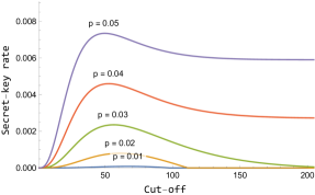
Figure 3: Secret-key rate with a global cut-off policy as a function of the cut-off parameter. Parameters used are $n=5$ and $\lambda=0.998$.

In Fig. 4 we show how such an optimization can be used for parameter exploration. There, we show the secret-key rate optimized over the global cut-off parameter as a function of the number of segments for several total distances. The parameters used are $\lambda=0.995$ and $\lambda_{\textrm{gen}}=0.999$, where the last parameter corresponds to imperfect state generation.

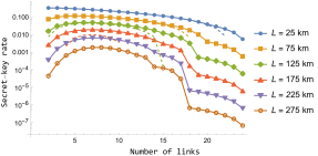
Figure 4: Secret-key rate optimized over the global cut-off parameter for several distances $L$. Parameters used are $\lambda=0.995$ and $\lambda_{\textrm{gen}}=0.999$. The dashed lines correspond to the secret-key rate without any cut-off. The abrupt behavior corresponds to the optimal cut-off changing.

IV Generating function approach

The methods from the previous section provide a recipe to calculate, at least in principle, an analytical form of the average noise. However, the expressions grow unwieldy very fast, seemingly without any structure to them kamin2023exact . Thus, while the recursive calculation allows for an exact, quantitative understanding of the noise in swap ASAP repeater chains, it does not directly yield a qualitative understanding.

In this section we show one method of overcoming this—the so-called generating function approach (not to be confused with the probability generating function). What is more, this approach also yields a computationally faster method to calculate the analytical formulae found with previous methods. We will first outline what a generating function is, and how it aids the understanding of noise in repeater chains. Afterwards, we investigate the found approximations, and use it for parameter explorations in repeater chains.

IV.1 Outline of the approach

Generating functions are the main object of study in analytic combinatorics flajolet2009analytic ; pemantle2013analytic . For our setting, the associated generating function has the form

$$G=G(x,\lambda,q)=\sum_{n=1}^{\infty}\mathds{E}\left[\Lambda_{n}\right]x^{n}\ ,$$ (13)

where $x$ can take complex values. The goal is to first find a closed-form expression $G$. Given such a closed-form expression, it is possible to extract complex analytic behavior about $G$. In turn, this analytic behavior of $G$ places strong constraints on the growth of $\mathds{E}\left[\Lambda_{n}\right]$. In particular, for fixed $\lambda$ and $q$, $G$ is a meromorphic function in $x$, and it is the singularity closest to the origin (specifically its location and residue) that dictates the growth of $\mathds{E}\left[\Lambda_{n}\right]$.

At this point, a remark is in order. It is not clear whether a nice closed-form expression for $G$ should exist, especially since we have argued that the individual coefficients $\mathds{E}\left[\Lambda_{n}\right]$ become unwieldy. This is, however, a powerful feature of generating functions — generating functions often behave much better than their coefficients considered individually flajolet2009analytic ; pemantle2013analytic . This well-behavedness is not only what allows us to extract information about the individual coefficients, but also allows us to find $G$ in the first place.

Using the recursive formulation from the previous section, we show in Appendix E that

$$G= ~{}x\cdot\Phi_{1}+x^{2}\left(\frac{\left(1-q\right)^{2}\lambda}{\left(\lambda-q\right)\left(1-\lambda q\right)}\right)\frac{\Phi_{2}\cdot\Phi_{4}}{1-x\cdot\Phi_{3}}\ ,$$ (14)

where the $\Phi_{i}=\Phi_{i}(x)=\Phi_{i}(x,\lambda,q)$ are particular instances of so-called $q$-hypergeometric series gasper2004basic , and are functions of $x$, $\lambda$ and $q$ (see Eqs. (109) to (114) for a full description). Since the $\Phi_{i}$ are all entire functions in $x$ for fixed $\lambda,q$ (with $\lambda\neq q$), the only singularity arises when $1-x\cdot\Phi_{3}=0$. Although understanding analytical solutions to equations involving ($q$-)hypergeometric series is generally a difficult endeavor driver2008zeros ; dominici2013real , it is straightforward to find solutions numerically. Let $\rho$ be the smallest real solution to $1-x\cdot\Phi_{3}=0$. Using standard results from analytic combinatorics (see, for example, the two principles of coefficient asymptotics in Chapter IV from flajolet2009analytic ) we find that

$$\mathds{E}\left[\Lambda_{n}\right]\sim\left[-\textrm{Res}_{\rho}\left(G\right)\right]\cdot\left(\frac{1}{\rho}\right)^{n+1}$$

$$=\left[\left(\frac{\left(1-q\right)^{2}\lambda\rho}{\left(\lambda-q\right)\left(1-\lambda q\right)}\right)\cdot\left(\frac{\Phi_{2}(\rho)\cdot\Phi_{4}(\rho)}{\Phi_{3}(\rho)+\rho\cdot\Phi_{3}^{\prime}(\rho)}\right)\right]\cdot\left(\frac{1}{\rho}\right)^{n}$$

$$\equiv\left[A(\lambda,q)\right]\cdot B(\lambda,q)^{n}\ ,$$ (15)

where $\textrm{Res}_{\rho}\left(f\right)$ is the residue of a function $f$ at $\rho$ and the $\sim$ means that the ratio between the two sides converges to $1$ as $n\rightarrow\infty$. The first equality follows from the fact that $\textrm{Res}_{\rho}\left(f/g\right)=\frac{f(\rho)}{g^{\prime}(\rho)}$ when $f,g$ are holomorphic on a disk containing $\rho$, and $\rho$ is a simple zero of $g$.

The approximation in Eq. (15) has a clear conceptual interpretation — the quality of the state decays exponentially in the number of segments $n$, where the decay factor is given by $B(\lambda,q)$ for each added segment. The $A(\lambda,q)$ term, on the other hand, can be thought of as a correction term. Note that both terms are independent of $n$. In the following subsection we numerically show that this approximation is not only tight in the asymptotic limit; it is already good enough for practical purposes for small $n$.

It is possible to approximate $\mathds{E}\left[\Lambda_{n}\right]$ by including more than just the singularity closest to the origin, leading to a sum of exponential terms flajolet2009analytic . In practice, we find that taking the first singularity suffices.

All of the above generalizes straightforwardly to the case of a global cut-off, where there exist analogous functions $\overline{A}(\lambda,q,T_{c})$ and $\overline{B}(\lambda,q,T_{c})$ as well — see Appendices E and E.3 for the derivation of the associated generating function.

We conclude this subsection with two remarks. First, with the generating function $G$ in hand, it is easier to find analytical expressions of $\mathds{E}\left[\Lambda_{n}\right]$ than with the recursive relation from Section III. This allows us to analytically calculate $\mathds{E}\left[\Lambda_{25}\right]$ in a matter of seconds with Mathematica —something that was impossible with the recursive approach mathematicafiles . Second, we note that the function $G$ is a multivariate generating function pemantle2013analytic , where the associated combinatorial object can be interpreted as a type of lattice path $L$. The associated parameters $q$, $\lambda$ and $x\left(\frac{1-q}{q}\right)$ count the area $A(L)$ under the path, the roughness $K(L)$ and the width $n(L)$ of the path, respectively. This result may be of independent interest to combinatorialists.

IV.2 Parameter exploration

In this subsection we will first explore the approximation found in Eq. (15), before using it to understand how $\lambda$ and $q$ affect $\mathds{E}\left[\Lambda_{n}\right]$ qualitatively.

Fig. 5 shows the difference between the exact average noise and Eq. (15) for four sets of values of $\lambda$ and $q$. We find that Eq. (15) gives an approximation that converges exponentially fast, independent of the parameters used.

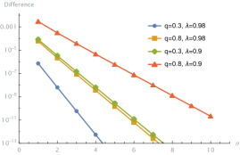
Figure 5: Difference between the approximation of Eq. (15) and the exact average noise parameter $\mathds{E}\left[\Lambda_{n}\right]$ as a function of $n$, for four different sets of parameters.

From Eq. (15) and Fig. 5 we find that $\mathds{E}\left[\Lambda_{n}\right]$ decays exponentially in the number of segments. In particular, $B\left(\lambda,q\right)$ can be thought of as a decay parameter — every additional segment added reduces the average $\Lambda$ parameter by a factor of $B\left(\lambda,q\right)$. The decay parameter thus allows us to assign a metric to a given repeater chain for a fixed $\lambda$ and $q$, independent of the number of segments.

As we show in Appendix E.3, a similar approximation works for the global cut-off as well. That is, we find a similar decay parameter $\overline{B}\left(\lambda,q,T_{c}\right)$, and analyze in Fig. 6 how $\overline{B}(\lambda,q,T_{c})$ varies as a function of $\lambda$ and $q$, for three values of the cut-off, $T_{c}=2$, $6$ and $10$. We find that the found tight approximation allows for a fast qualitative understanding of noise in swap ASAP repeater chains, which would have been impossible through a Monte Carlo simulation.

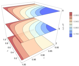
Figure 6: Several slices of the $\overline{B}(\lambda,q,T_{c})$ function for $T_{c}=2,6,10$. The $\overline{B}(\lambda,q,T_{c})$ is a proxy for the decay rate of the quality of the state as additional segments get added.

V Distribution of the noise

In this section we will show that knowing $\mathds{E}\left[\Lambda_{n}\right]$ is, in principle, enough to reconstruct the underlying probability distribution of the $\Lambda_{n}$ parameter. We then apply our results to a so-called ‘binning’ approach to quantum key distribution.

V.1 Derivation

We will use here the found analytical forms of $\mathds{E}\left[\Lambda_{n}\right]$ to find the actual distribution of the noise. As noted before in the paper and in kamin2023exact , the key insight is that $\mathbb{E}\left[\Lambda_{n}\right]$ is the probability generating function (not to be confused with the generating function from the previous section) of the random variable corresponding to the roughness $K$. That is,

$$\mathbb{E}\left[\Lambda_{n}\right]= ~{}\left(\frac{1-q}{q}\right)^{n}\sum_{\overline{t}}\left(q^{\sum_{i}^{n}t_{i}}\right)\cdot\left(\lambda^{\sum_{i}^{n-1}\left|t_{i}-t_{i+1}\right|}\right)$$

$$= ~{}\sum_{k=0}^{\infty}P\left(K=k\right)\lambda^{k}$$

$$= ~{}\sum_{k=0}P\left(\Lambda_{n}=\lambda^{k}\right)\lambda^{k}\ .$$

From this it follows that

$$k!\cdot P\left(\Lambda_{n}=\lambda^{k}\right)=\left.\left(\mathds{E}\left[\lambda_{n}\right]^{(k)}\right)\right|_{\lambda=0}\ .$$ (16)

Here $\mathds{E}\left[\Lambda_{n}\right]^{(k)}$ is the $k$’th derivative of $\mathds{E}\left[\Lambda_{n}\right]$, which is understood to be with respect to $\lambda$. Using Mathematica, $P\left(\Lambda_{n}=\lambda^{k}\right)$ can be calculated analytically for all $k$ for up to $n=10$ segments mathematicafiles .

In Fig. 7, we validate our analytical results by using a Monte Carlo simulation. That is, we compare the exact distribution $P(K=k)$ of the roughness for $6$ segments and $q=0.6$, and compare it with an estimate of the distribution from a Monte Carlo simulation over $10^{5}$ timesteps. We already see excellent agreement, and we find convergence to the analytical distribution as we increase the number of runs. One interesting feature is the ‘non-smooth’ behavior of $P(K=k)$ (e.g. $P(K=6)\geq P(K=7)$, but $P(K=7)\leq P(K=8)$) which becomes more pronounced for larger $p$.

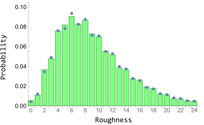
Figure 7: Verification of the analytical distribution of the roughness $K=\sum_{i=1}^{n-1}\left|t_{i}-t_{i+1}\right|$ for $q=0.6$ and $n=6$ segments (blue markers), along with an estimation found through a Monte Carlo simulation over $10^{5}$ runs (green bars). The Monte Carlo simulation converges to the exact distribution as the number of runs increases.

Using that $P(K=k)=P(\Lambda_{n}=\lambda^{k})$, we show in Fig. 8 the distribution of $\Lambda_{n}$ for $p=0.1$ and $\lambda=0.995$ for $n$ ranging from $2$ to $10$. Note that the ‘non-smooth’ behavior has disappeared since $p$ is relatively small.

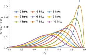
Figure 8: Distribution of the final $\Lambda_{n}$ parameter for $q=0.9$, $\lambda=0.995$ for several number of segments.

In principle a similar approach would work for the case with a global cut-off; however, due to the associated expressions becoming more complex, it was not possible to find analytical expressions of the $k$’th derivative.

V.2 Parameter exploration

As an application of the analytical expressions of the distribution on $\Lambda_{n}$, we consider secret key generation with a so-called binning method; see, for example, jing2020quantum ; goodenough2023near . That is, the collected classical data are separated into ‘bins’ according to the available information about the associated generated state. Here, this available information would contain the roughness parameter $K(\overline{t})$, which describes the quality of the state Note that the data need not be received at the time of measurement, which would have come at the cost of increased decoherence.

How does this binning help? Let $\textrm{SKF}\left(\Lambda\right)$ be the secret-key fraction, i.e. the fraction of bits that can be extracted from an asymptotic number of copies of a state with parameter $\Lambda$ (see Appendix D for more information). Without binning, the secret-key fraction is given by $\textrm{SKF}\left(\mathds{E}\left[\Lambda\right]\right)$. With binning, the secret-key fraction becomes the weighted average. That is,

$$\sum_{k=0}^{\infty}P(\Lambda=\lambda^{k})\cdot\textrm{SKF}\left(\lambda^{k}\right)$$ (17)

$$= \sum_{k=0}^{k_{\textrm{max}}}P(\Lambda=\lambda^{k})\cdot\textrm{SKF}\left(\lambda^{k}\right)$$

$$\geq \,\textrm{SKF}\left(\mathds{E}\left[\Lambda\right]\right)\ ,$$

where in the first step we used that the secret-key fraction is zero for $\Lambda\leq\Lambda_{\textrm{min}}\approx 0.778$, such that $k_{\textrm{max}}=\left\lceil\frac{\log(\Lambda_{\textrm{min}})}{\log(\lambda)}\right\rceil$. In the second step, we used that the secret-key fraction is convex as a function of $\Lambda$.

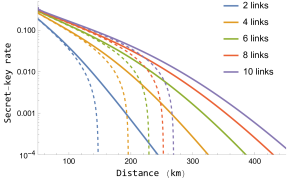
Figure 9: Secret-key rate with (solid) and without (dashed) a binning strategy (see main text) as a function of the distance, for several number of segments $n$ and $\lambda=0.99$.

Fig. 9 shows the secret-key rate both with and without the binning method as a function of the distance. The data shown correspond to $\lambda=0.99$ and several values of $n$. We observe that the secret-key rate can be non-zero for any arbitrary distance. This should not come as a surprise — the probability $P(K=0)=\sum_{t=1}^{\infty}\left(p\left(1-p\right)^{t-1}\right)^{n}=\frac{p^{n}}{1-(1-p)^{n}}\approx p^{n}$ is small but strictly positive for any $p>0$.

VI Discussion

In this work we have characterized the noise in homogeneous swap ASAP repeater chains. We have done so by providing analytical formulae and tight approximations of the average fidelity (even when considering a global cut-off) along with the complete distribution of the noise, for a general class of noise models. The numerical evaluation of the formulae goes beyond existing work and reaches 25 repeater segments if one is interested in the average fidelity of the end-to-end link only, and to 10 repeater segments for a full characterization of the noise distribution. Since near-term quantum repeater experiments will most likely be based on swapping as soon as possible together with a cut-off policy, these results yield an understanding of what to expect for near-term networks. In particular, the optimization of the global cut-off (which would once be a costly Monte Carlo simulation) can now be done efficiently.

Due to the flexibility of the generating function approach, we anticipate that similar techniques as used here can be applied to other entanglement distribution problems, such as in avis2023analysis .

In follow-up work, we investigate both the inhomogeneous bipartite setting and the inhomogeneous multipartite setting. This follow-up work hinges on interpreting Eq. (12) as the (classical) partition function of a particular physical system — the solid-on-solid model owczarek1993exact ; rozycki2003rsos ; owczarek2009exact ; owczarek2010exact . By then exploiting techniques from statistical physics, we find numerically tight approximations on the average noise.

There are still two open questions. First, is there a way to extend the generating function approach to incorporate the additional noise on Alice’s and Bob’s memories? Using Jensen’s inequality, one can provide a lower bound, but an analytical solution seems currently out of reach. Secondly, there are also other swapping schemes and cut-off policies besides the global cut-off that are amenable to an analytical approach, as have been treated for QKD in kamin2023exact . It would be of both quantum and combinatorial interest to find associated generating functions that capture Alice’s and Bob’s noise and/or the other cut-off policies.

Appendix A Other cut-off policies

For completeness, we mention here several other cut-off policies, but which will not be considered in this paper. As previously mentioned, decoherence is a prime obstacle to quantum communication. A cut-off policy is a condition for discarding the present entanglement. Discarding the generated entanglement will reduce the rate at which entanglement is delivered, but will mitigate the time spent on distributing end-to-end entanglement which is of too low quality. A cut-off policy thus allows for a trade-off between the rate and the quality of the delivered end-to-end entanglement. Cut-off policies and their trade-offs have been studied in for example rozpkedek2018parameter ; rozpkedek2019near ; collins2007multiplexed ; avis2022requirements ; li2020efficient ; kamin2023exact ; shchukin2019waiting ; reiss2023deep , where they were shown to be indispensable for near-term devices.

The local cut-off policy limits the time a single memory is allowed to store entanglement for. As soon as a memory not belonging to Alice or Bob holds entanglement, a timer is started. As before, this timer increases by $1$ every round, and is reset to $0$ after discarding. A reset occurs when any timer exceeds $T_{c}$, where we use the same notation for the global and local cut-off. In Fig. 10 we show an example of the local cut-off. Here, the left memory of the fourth link had to store entanglement for more than $T_{c}=2$ rounds.

Figure 10: Graphical description of the local cut-off policy. Each node has agreed on a parameter $T_{c}$. For the local cut-off, a reset is performed when any node has to store entanglement for more than $T_{c}$ rounds. We consider the local cut-off in follow-up work.

The policy considered in praxmeyer2013reposition is similar to the global cut-off policy in this paper. However, instead of starting a timer at the beginning of all attempts, a timer is started at the time the first link succeeds. Another policy would be based on predicting the delivery time (see inesta2023optimal ) and quality of the delivered state, conditioned on the current state of the repeater chain inesta2023optimal . Note that all entanglement is reset after a cut-off condition has been reached in the policy of praxmeyer2013reposition and both the global and local cut-off.

We have numerically observed through Monte Carlo simulations that the local cut-off performs slightly better than the global cut-off, but not by a significant amount.

Appendix B Generalization to $X$-symmetric qudit Pauli noise

Our analysis in the main text is based on the depolarizing channel as noise model for memory decoherence (see Section II). There were two key features of this noise model that made it amenable for analysis:

1. The key parameter multiplies when composing two noise channels. The depolarizing noise model from Section II is parameterized by two values: the probability of preserving the state perfectly (i.e. $\lambda$) and the probability of transforming the state into the maximally mixed state. Due to normalization, this last probability is just $1-\lambda$. Applying a noise map with a given $\lambda_{\textrm{noise}}$ corresponds to the transformations $\lambda\rightarrow\lambda\cdot\lambda_{\textrm{noise}}$ and $1-\lambda\rightarrow 1-\lambda\cdot\lambda_{\textrm{noise}}$. The fact that the first map corresponds to multiplication was a key part of our analysis.

2. The key parameter multiplies when performing the entanglement swap. Next, we used the fact that performing a swap between two states described by noise parameters $\lambda$ and $\lambda^{\prime}$, respectively, leads to a new state with noise parameter $\lambda\cdot\lambda^{\prime}$.

In this Appendix, we will consider the more general scenario where the nodes hold two-qudit entangled states. We will show for a large class of qudit channels that we call $X$-symmetric channels, how to find a parameterization into parameters $\vec{\lambda}$ such that the two above properties still hold. To be precise, an $X$-symmetric channel $\mathcal{N}$ is a $d$-dimensional qudit Pauli channel (definition below in Section B.1) for which $p_{X^{a}Z^{b}}=p_{X^{-a}Z^{b}}$ for all $a,b\in\{0,1,\dots,d-1\}$. We will give a procedure how to find a parameterization $\mathcal{N}=\mathcal{N}_{\vec{\lambda}}$ into at most $d^{2}$ parameters $\vec{\lambda}=(\lambda_{1},\lambda_{2},\dots,\lambda_{d^{n}})$, such that both composition (item 1 below) and entanglement swapping (item 2) are represented by pointwise multiplication of the entries of $\vec{\lambda}$:

1. for any two $\vec{\lambda},\vec{\lambda}^{\prime}$, we have $\mathcal{N}_{\vec{\lambda}}\circ\mathcal{N}_{\vec{\lambda}^{\prime}}=\mathcal{N}_{\vec{\lambda}\cdot\vec{\lambda}^{\prime}}$.

2. let $\psi_{d}=\ket{\psi_{d}}\bra{\psi_{d}}$ be a maximally-entangled states on two $d$-dimensional qudits. Then for any two $\vec{\lambda},\vec{\lambda}^{\prime}$, an entanglement swap on states $(\mathds{I}\otimes\mathcal{N}_{\vec{\lambda}})\left[\psi\right]$ and $(\mathds{I}\otimes\mathcal{N}_{\vec{\lambda}^{\prime}})\left[\psi_{d}\right]$ yields the state $(\mathds{I}\otimes\mathcal{N}_{\vec{\lambda}\cdot\vec{\lambda}^{\prime}})\left[\psi_{d}\right]$.

where $\vec{\lambda}\cdot\vec{\lambda}^{\prime}=(\lambda_{1}\lambda_{1}^{\prime},\ldots,\lambda_{d^{2}}\lambda_{d^{2}}^{\prime})$ represents entrywise multiplication and $\mathds{I}$ is the $d$-dimensional qudit identity channel.

Consequently, the analysis in the main text is straightforwardly extendible to qudit links as long as the noise model is an $X$-symmetric channel. The $X$-symmetric channels form a subset of qudit Pauli channels, and include (biased) depolarizing noise as well as any qubit Pauli channel (i.e. Pauli channels for $d=2$).

In what follows we first recall the definition of qudit Pauli channels. We then study composition of qudit Pauli channels, and show that qudit Pauli channels admit a parameterization so that channel composition is represented by multiplication of the parameters. Finally, we investigate how maximally entangled states that have undergone qudit Pauli channels are transformed under swap operations. From the latter, we infer that in general, the entanglement swap is not represented by parameter multiplication, but for $X$-symmetric channels, it is.

B.1 Qudit Pauli channels

A qudit Pauli channel is any channel $\mathcal{N}$ corresponding to a probabilistic mixture of operators from the set $\mathcal{U}=\{{X^{a}Z^{b}\}}_{a,b=0}^{d-1}$ shahbeigi2021log , i.e.

$$\mathcal{N}\left(\cdot\right)=\sum_{U\in\mathcal{U}}p_{U}U\left(\cdot\right)\ .$$ (18)

Here $0\leq a\leq d-1$, $0\leq b\leq d-1$ shahbeigi2021log , and $X$ and $Z$ are generalized Pauli operators defined by their action on the standard basis of $\mathbb{C}^{d}$,

$$X\ket{j} =\ket{j+1\mod d}\ ,$$ (19)

$$Z\ket{j} =\omega^{j}\ket{j}\ ,$$ (20)

where $\omega=e^{\frac{2\pi i}{d}}$ weyl1927quantenmechanik .

Note that $X^{a}Z^{b}$ and $X^{k}Z^{l}$ commute up to a phase. Since $ABA^{\dagger}=\left(e^{i\theta}A\right)B\left(e^{i\theta}A\right)^{\dagger}$ for any angle $\theta\in[0,2\pi)$, we have that $\left(X^{a}Z^{b}\right)\left(X^{k}Z^{l}\right)\rho\left(\left(X^{a}Z^{b}\right)\left(X^{k}Z^{l}\right)\right)^{\dagger}=\left(X^{k}Z^{l}\right)\left(X^{a}Z^{b}\right)\rho\left(\left(X^{k}Z^{l}\right)\left(X^{a}Z^{b}\right)\right)^{\dagger}$; qudit Pauli channels commute. Now equip the set $\mathcal{U}$ with a group structure, where the group operation is given by matrix multiplication but where phases are ignored. Formally, this is the group ${\raisebox{1.99997pt}{$\langle X,Z\rangle$}\left/\raisebox{-1.99997pt}{$\langle\omega I\rangle$}\right.}$, of which $\{{X^{a}Z^{b}\}}_{a,b=0}^{d-1}$ forms a transversal of the underlying equivalence relation. This group is isomorphic to $C_{d}\times C_{d}$, the direct product of the cyclic group of order $d$ with itself.

B.2 Mapping composition of qudit Pauli channels to multiplication

We first investigate the composition of two qudit Pauli channels, where in particular we are interested in reducing the composition to multiplication of real numbers, i.e. the analogues of the $\lambda$ parameter for qubit depolarizing noise. The composition of two channels $\mathcal{N}_{1},\mathcal{N}_{2}$ with distributions $p_{U}\equiv f(U)$ and $p_{U}\equiv g(U)$, respectively, can be written as

$$\left(\mathcal{N}_{2}\circ\mathcal{N}_{1}\right)\left[\cdot\right] =\sum_{U\in\mathcal{U}}g(U)U\left[\sum_{V\in\mathcal{U}}f(V)V\left[\cdot\right]\right]$$ (21)

$$=\sum_{W\in\mathcal{U}}\left(\sum_{UV=W}g(U)f(V)\right)W\left[\cdot\right]\ .$$ (22)

We recognize eq. (22) as a convolution over finite Abelian groups. The Fourier transform of a function $h:\mathcal{G}\rightarrow\mathbb{C}$, where $\mathcal{G}$ is a finite Abelian group, is defined as the function $\hat{h}:\hat{\mathcal{G}}\rightarrow\mathbb{C}$ such that

$$\hat{h}\left(\chi\right)=\sum_{U\in\mathcal{G}}h(U)\chi(U)^{*}\ .$$

The inverse Fourier transform is given by

$$h(U)=\frac{1}{\left|\mathcal{G}\right|}\sum_{\chi\in\hat{\mathcal{G}}}\hat{h}(\chi)\chi(U)\ .$$ (23)

Here, the $\chi$ are also called the (unitary) characters of $\mathcal{G}$, i.e. the distinct homomorphisms from $\mathcal{G}$ to the group of unit complex numbers $\mathbb{T}=\{z\in\mathbb{C}\mid\left|z\right|=1\}$. That is, the set of all functions $\chi:\mathcal{G}\rightarrow T$ such that $\chi\left(U\right)\chi\left(V\right)=\chi\left(UV\right)$. We denoted by $\hat{\mathcal{G}}$ the set of all characters of $\mathcal{G}$.

The procedure to find the desired parameterization now is as follows. First, we recall that the coefficients of the channel are specified through the noise coefficient map $f$, defined as $f(U)=p_{U}$, where $U$ is an element of the phaseless qudit Pauli group $\mathcal{U}$. The first step is to compute the Fourier transform of $f$. The second step to determine the characters $\chi$ of $\mathcal{U}$. These are the same as the characters of $C_{d}\times C_{d}$, to which the phaseless Pauli group $\mathcal{U}$ is isomorphic; in turn, we can derive the characters of $C_{d}\times C_{d}$ from the characters of $C_{d}$ isaacs2006character . Finally, we evaluate the Fourier transform $\hat{f}$ at the characters $\chi$. We will choose the resulting $\hat{f}(\chi)$ as our new parameters $\lambda_{1},\lambda_{2},\ldots$, as convolution of two functions becomes pointwise multiplication of their Fourier transforms terras1999fourier ; diaconis1988group .

As special case, we consider $d=2$, i.e. we consider an arbitrary qubit Pauli channel. In that case, $\mathcal{U}$ is isomorphic to $C_{2}\times C_{2}$ (also known as the Klein four-group), which has characters

$$\chi^{1}(I) =1,\quad\chi^{1}(X) =1,\quad \chi^{1}(Y)=1,\quad \chi^{1}(Z)=1\ ,$$

$$\chi^{2}(I) =1,\quad\chi^{2}(X) =1,\quad \chi^{2}(Y)=-1,\quad \chi^{2}(Z)=-1\ ,$$

$$\chi^{3}(I) =1,\quad\chi^{3}(X) =-1,\quad \chi^{3}(Y)=1,\quad \chi^{3}(Z)=-1\ ,$$

$$\chi^{4}(I) =1,\quad\chi^{4}(X) =-1,\quad \chi^{4}(Y)=-1,\quad \chi^{4}(Z)=1\ .$$

From normalization of the probability, we see that $\lambda_{1}$ is always equal to 1. The remaining parameters are

$$\lambda_{2}=p_{I}+p_{X}-p_{Y}-p_{Z}\ ,$$ (24)

$$\lambda_{3}=p_{I}-p_{X}+p_{Y}-p_{Z}\ ,$$ (25)

$$\lambda_{4}=p_{I}-p_{X}-p_{Y}+p_{Z}\ \$$ (26)

which is indeed the parameterization given in the main text in Section II.

Let us specialize to the case of depolarizing noise, where $p_{X}=p_{Y}=p_{Z}=\frac{1-p_{I}}{3}$. We then see that $\lambda^{2}=\lambda^{3}=\lambda^{4}=p_{I}-\frac{1-p_{I}}{3}=\frac{4p_{I}-1}{3}=\frac{4F-1}{3}$, which we see is the original $\lambda$ treated in the main text.

B.3 Swapping of states

Let $\ket{\psi_{d}}\equiv\frac{1}{\sqrt{d}}\sum_{i=0}^{d-1}\ket{ii}$ be a qudit maximally entangled state and set $\ket{\psi_{d}}\bra{\psi_{d}}\equiv\psi_{d}$. Let $\mathcal{N}$ be a qudit Pauli channel acting on one-half of a qudit maximally entangled state. We will first show that the side the channel acts on is immaterial (i.e. $\mathds{I}\otimes\mathcal{N}\left[\psi_{d}\right]=\mathcal{N}\otimes\mathds{I}\left[\psi_{d}\right]$) if $\mathcal{N}$ is $X$-symmetric (which we define shortly). Thus even if $X$-symmetric noise has acted on both sides of $\ket{\psi_{d}}$, we are free to pretend there is one qudit Pauli channel $\mathcal{N}$ acting on an arbitrary side, yielding a state $\mathds{I}\otimes\mathcal{N}\left[\psi_{d}\right]=\mathcal{N}\otimes\mathds{I}\left[\psi_{d}\right]\equiv\rho_{\mathcal{N}}$. Secondly, we will show that swapping two states $\rho_{\mathcal{N}_{1}},\rho_{\mathcal{N}_{2}}$ yields a state $\rho_{\left(\mathcal{N}_{1}\circ\mathcal{N}_{2}\right)}$.

B.3.1 Transpose trick for $X$ symmetric channels

The well-known transpose trick wilde2011classical states that if $A$ is any square matrix (of the appropriate size), the following holds

$$\mathds{I}\otimes A\ket{\psi_{d}}=A^{\mathsf{T}}\otimes\mathds{I}\ket{\psi_{d}}\ .$$ (27)

Here $A^{\mathsf{T}}$ is the transpose of $A$ with respect to the basis $\{{\ket{i}\}}_{i=1}^{d-1}$. Applying the transpose trick to $\mathds{I}\otimes\mathcal{N}\left[\psi_{d}\right]$ yields

$$\mathds{I}\otimes\mathcal{N}\left[\psi_{d}\right] =\sum_{a,b=0}^{d-1}p_{X^{a}Z^{b}}\left(\mathds{I}\otimes X^{a}Z^{b}\right)\left[\psi\right]$$ (28)

$$=\sum_{a,b=0}^{d-1}p_{X^{a}Z^{b}}\left(\left(X^{a}Z^{b}\right)^{\mathsf{T}}\otimes\mathds{I}\right)\left[\psi\right]$$ (29)

$$=\sum_{a,b=0}^{d-1}p_{X^{a}Z^{b}}\left(X^{-a}Z^{b}\otimes\mathds{I}\right)\left[\psi\right]\ ,$$ (30)

where we used that $\left(X^{a}Z^{b}\right)^{\mathsf{T}}=Z^{b}X^{-a}$, which is equal to $X^{-a}Z^{b}$ up to a phase.

The above implies that the side a qudit Pauli channel is applied to is immaterial if and only if $p_{X^{a}Z^{b}}=p_{X^{-a}Z^{b}}$. This means that the condition holds when the probability of applying $X^{a}Z^{b}$ is equal to the probability of applying $X^{-a}Z^{b}$. This property holds for several relevant classes of channels, such as arbitrary qubit Pauli channels, arbitrary qudit dephasing noise (since the probability of applying $X^{a}Z^{b}$ is zero when $a\neq 0$) and qudit depolarizing noise.

Figure 11: Graphical description of the proof of the desired properties of $X$-symmetric channels. From a) to b) we use the transpose trick to show that the side on which the noise is applied is immaterial. From b) to c) we use that the application of the noise and the Bell state measurement commute. From c) to d) we performed the projection into one of the (generalized) Bell states. From d) to e) we use the commutativity of qudit Pauli operators (up to a phase). From e) to f) we use the transpose trick again to move the noise all to one side.

B.3.2 Swapping of $X$-symmetric noisy states

In the previous section we have shown that we have the freedom to move $X$-symmetric channels from one side of the maximally entangled state to the other. With this tool in hand, let us perform a swap on two such noisy states, see Fig. 11. In a) we show the complete procedure of swapping, including the measurement and classical correction. We have assumed without loss of generality that the channels $\mathcal{N}_{1}$ and $\mathcal{N}_{2}$ act on the qudits on which the Bell state measurement (green triangle) is performed. After the Bell state measurement, a classical outcome $k$ is recorded, and is used to specify which correction $U_{k}^{\dagger}$ needs to be performed on one of the sides after measuring. Note that the corrections $U_{k}^{\dagger}$ are generalized Pauli operators.

In step b) we use the result from the previous section that we are free to move $X$-symmetric channels to the other side. In step c), we commute the Bell state measurement and the channels, which is allowed since the operations act on different qubits. In step d) we use that measuring outcome $k$ projects the state unto $\mathds{I}\otimes U_{k}\ket{\psi_{d}}$. From d) to e) we use that the qudit Pauli operators commute (up to an immaterial phase), and finally we use that $X$-symmetric channels can be moved freely between the two sides.

We close with one final remark. The average values for the $\lambda_{i}$ parameters can be interpreted as the $\lambda_{i}$ parameters of the average channel acting on the entangled state shared between Alice and Bob. This is because convex combinations of qudit Pauli channels map exactly to convex combinations of the $\vec{\lambda}$, since the Fourier transform is linear.

Appendix C Recursion calculations

Here we provide the details for the recursive calculation for the analytics of the average noise parameter.

C.1 Recursion calculation without a cut-off policy

As discussed in Section III, calculating the average $\Lambda_{n}$ parameter requires us first to express $H_{n}^{t}$ recursively, from which $H_{n}\equiv\mathds{E}\left[\Lambda_{n}\right]$ can be found. The main idea is to express the map from $H_{n}^{t}$ to $H_{n+1}^{t}$ in terms of a linear transformation on the real vector space spanned by $q^{at}\lambda^{bt},~{}a,b\in\mathbb{Z}$. That is, all finite linear combinations of the form $\sum_{m}c_{a,b}q^{at}\lambda^{bt}$, where $c_{a,b}\in\mathbb{R}$.

As a warm-up, let us consider the first recursion step. Here and in what follows, we will drop the $\frac{1-q}{q}$ prefactor, i.e. we set

$$Z_{n} =\sum_{\overline{t}}\left(q^{\sum_{i=1}^{n}t_{i}}\right)\cdot\left(\lambda^{\sum_{i=1}^{n-1}\left|t_{i}-t_{i+1}\right|}\right)$$ (31)

$$Z_{n}^{t} =\sum_{\mathclap{\begin{subarray}{c}\overline{t}~{}\textrm{s.t.}\\ t_{n}=t\end{subarray}}}\left(q^{\sum_{i=1}^{n}t_{i}}\right)\cdot\left(\lambda^{\sum_{i=1}^{n-1}\left|t_{i}-t_{i+1}\right|}\right)\ ,$$ (32)

such that $H_{n}=\left(\frac{1-q}{q}\right)^{n}Z_{n}$. Note that $Z_{1}^{t}$ is given by $q^{t}$, since there is only the associated probability of succeeding at time $t$ and no decoherence.

Let $M$ correspond to the map in the recursion, i.e. the map $Z_{i}^{t}\xrightarrow{M}Z_{i+1}^{t}$. We then have for the first step that

$$Z_{1}^{t}\xrightarrow{M}Z_{2}^{t}= \sum_{t^{\prime}=1}^{\infty}q^{t}\lambda^{\left|t-t^{\prime}\right|}Z_{1}^{t^{\prime}}$$ (33)

$$= \left(\,\sum_{t^{\prime}=1}^{t-1}q^{t}\lambda^{t-t^{\prime}}Z_{1}^{t^{\prime}}\right)+\left(\,\sum_{t^{\prime}=t}^{\infty}q^{t}\lambda^{t^{\prime}-t}Z_{1}^{t^{\prime}}\right)$$ (34)

$$= \left(\,\sum_{t^{\prime}=1}^{t-1}q^{t}\lambda^{t-t^{\prime}}q^{t^{\prime}}\right)+\left(\,\sum_{t^{\prime}=t}^{\infty}q^{t}\lambda^{t^{\prime}-t}q^{t^{\prime}}\right)$$ (35)

$$= ~{}q^{t}\lambda^{t}\left(\,\sum_{t^{\prime}=1}^{t-1}\left(\frac{q}{\lambda}\right)^{t^{\prime}}\right)+\left(\frac{q}{\lambda}\right)^{t}\left(\,\sum_{t^{\prime}=t}^{\infty}\left(q\lambda\right)^{t^{\prime}}\right)$$ (36)

$$= ~{}q^{t}\lambda^{t}\left(\frac{\frac{q}{\lambda}-\left(\frac{q}{\lambda}\right)^{t}}{1-\frac{q}{\lambda}}\right)+\left(\frac{q}{\lambda}\right)^{t}\left(\frac{q\lambda-\left(q\lambda\right)^{t}}{1-q\lambda}\right)$$ (37)

$$= \left(-\frac{q\left(\frac{1}{\lambda}-\lambda\right)}{\left(1-\lambda^{-1}q\right)\left(1-\lambda q\right)}\right)\cdot q^{2t}\lambda^{0t}+\frac{q}{\lambda-q}\cdot q^{t}\lambda^{t}\ .$$ (38)

Note that the limit as $q$ goes to $\lambda$ and the limit of $q$ goes $\frac{1}{\lambda}$ exists. Observe that we end up with a linear combination of terms of the form $q^{at}\lambda^{bt}$. This is not specific to starting with $Z_{1}^{t}=q^{t}$, as we see in the following,

$$q^{at}\lambda^{bt}\xrightarrow{M} \sum_{t^{\prime}=1}^{\infty}q^{t}\lambda^{\left|t-t^{\prime}\right|}\cdot\left(q^{at^{\prime}}\lambda^{bt^{\prime}}\right)$$ (39)

$$= \left(\,\sum_{t^{\prime}=1}^{t-1}q^{t}\lambda^{t-t^{\prime}}\cdot\left(q^{at^{\prime}}\lambda^{bt^{\prime}}\right)\right)+\left(\,\sum_{t^{\prime}=t}^{\infty}q^{t}\lambda^{t^{\prime}-t}\cdot\left(q^{at^{\prime}}\lambda^{bt^{\prime}}\right)\right)$$ (40)

$$= ~{}C^{a,b}q^{\left(a+1\right)t}\lambda^{bt}+D^{a,b}q^{t}\lambda^{t}\ ,$$ (41)

where

$$C^{a,b} =-\frac{q^{a}\lambda^{b}\left(\frac{1}{\lambda}-\lambda\right)}{\left(1-\lambda^{b-1}q^{a}\right)\left(1-\lambda^{b+1}q^{a}\right)}\$$ (42)

$$D^{a,b} =\frac{q^{a}}{\lambda^{1-b}-q^{a}}\ .$$ (43)

The $C^{a,b}$ and $D^{a,b}$ depend only on the values of $a,b\in\mathbb{Z}$ and $q$ and $\lambda$.

We can think of the $q^{at}\lambda^{bt}\equiv\ket{a,b}$ for $a,b\in\mathbb{Z}$ as the basis vectors of a vector space $V$. The map $M$ defined for an arbitrary $\ket{a,b}$ is, in fact, a linear map from $V$ to $V$, and so works for all expressions that are sums of terms of the form $q^{at}\lambda^{bt}$.

This allows us to calculate $Z_{n}^{t}$ fast. Setting $q^{at}\lambda^{bt}\equiv\ket{a,b}$, the map $M$ takes $\ket{a,b}$ to $C^{a,b}\ket{a+1,b}+D^{a,b}\ket{1,1}$. As such, we find that

$$Z_{1}^{t}=\ket{1,0}$$ (44)

$$\xrightarrow{M}Z_{2}^{t}=C^{1,0}\ket{2,0}+D^{1,0}\ket{1,1}$$ (45)

$$\xrightarrow{M}Z_{3}^{t}=C^{1,0}\left(C^{2,0}\ket{3,0}+D^{2,0}\ket{1,1}\right)+D^{1,0}\left(C^{1,1}\ket{2,1}+D^{1,1}\ket{1,1}\right)$$ (46)

$$=C^{1,0}C^{2,0}\ket{3,0}+D^{1,0}C^{1,1}\ket{2,1}+\left(C^{1,0}D^{2,0}+D^{1,0}D^{1,1}\right)\ket{1,1}\ .$$ (47)

This already gives us a method to fairly straightforwardly compute $Z_{n}^{t}$, especially when done on a computer.

Finally, we need to extract $Z_{n}^{t}$ from $Z_{n}$. Fortunately, since

$$\sum_{t=1}^{\infty}q^{at}\lambda^{bt}=\frac{q^{a}\lambda^{b}}{1-q^{a}\lambda^{b}}\ ,$$ (48)

this can be seen as a linear form defined on the basis vectors by $\ket{a,b}\mapsto\frac{q^{a}\lambda^{b}}{1-q^{a}\lambda^{b}}$. Using the above idea and equation (47), we find that the expectation value for $\Lambda_{3}$ for a homogeneous repeater chain of three segments is given by

$$\mathds{E}\left[\Lambda_{3}\right]=\left(\frac{1-q}{q}\right)^{3}\left(C^{1,0}C^{2,0}\frac{q^{3}}{1-q^{3}}+D^{1,0}C^{1,1}\frac{q^{2}\lambda}{1-q^{2}\lambda}+\left(C^{1,0}D^{2,0}+D^{1,0}D^{1,1}\right)\frac{q\lambda}{1-q\lambda}\right)\ .$$ (49)

C.2 Recursion calculation with a global cut-off policy

We take the same approach as in the previous section; the only difference now is that $t^{\prime}$ ranges from $1$ to $T_{c}$. Define

$$\bar{Z}_{n}^{t} =\sum_{\mathclap{\begin{subarray}{c}\overline{t}~{}\textrm{s.t.}\\ t_{n}=t\\ t_{i}\leq T_{c}\end{subarray}}}\left(q^{\sum_{i}^{n}t_{i}}\right)\cdot\left(\lambda^{\sum_{i}^{n-1}\left|t_{i}-t_{i+1}\right|}\right)\ ,$$ (50)

such that $\bar{Z}_{n}=\sum_{t=1}^{T_{c}}\bar{Z}_{n}^{t}$ and $\bar{H}_{n}=\left(\frac{1-q}{q\left(1-q^{T_{c}}\right)}\right)^{n}\bar{Z}_{n}$.

This gives the following recursion relation,

$$q^{at}\lambda^{bt}\xrightarrow{\bar{M}} \sum_{t^{\prime}=1}^{T_{c}}q^{t}\lambda^{\left|t-t^{\prime}\right|}\cdot\left(q^{at^{\prime}}\lambda^{bt^{\prime}}\right)$$ (51)

$$= \left(\sum_{t^{\prime}=1}^{t-1}q^{t}\lambda^{t-t^{\prime}}\cdot\left(q^{at^{\prime}}\lambda^{bt^{\prime}}\right)\right)+\left(\sum_{t^{\prime}=t}^{T_{c}}q^{t}\lambda^{t^{\prime}-t}\cdot\left(q^{at^{\prime}}\lambda^{bt^{\prime}}\right)\right)$$ (52)

$$= ~{}C^{a,b}q^{\left(a+1\right)t}\lambda^{bt}+D^{a,b}q^{t}\lambda^{t}+E^{a,b}q^{t}\lambda^{-t}$$ (53)

$$= ~{}C^{a,b}\ket{a+1,b}+D^{a,b}\ket{1,1}+E^{a,b}\ket{1,-1}\ ,$$ (54)

where $C^{a,b}$ and $D^{a,b}$ are as before and

$$E^{a,b}=-\frac{q^{a(1+T_{c})}\lambda^{\left(b+1\right)\left(T_{c}+1\right)}}{1-\lambda^{b+1}q^{a}}\ .$$ (55)

As in the previous section, by repeating this map $\bar{Z}_{n}^{t}$ can be calculated. Finally, since $\sum_{t^{\prime}=1}^{T_{c}}q^{at}\lambda^{bt}=\frac{q^{a}\lambda^{b}-q^{a\left(T_{c}+1\right)}\lambda^{b\left(T_{c}+1\right)}}{1-q^{a}\lambda^{b}}$ we find that the linear form that takes $\bar{Z}_{n}^{t}$ to $\bar{Z}_{n}$ is defined by $\ket{a,b}\mapsto\frac{q^{a}\lambda^{b}-q^{a\left(T_{c}+1\right)}\lambda^{b\left(T_{c}+1\right)}}{1-q^{a}\lambda^{b}}$.

Appendix D Expected delivery time and secret-key rate calculation

The secret-key rate is defined as the ratio between the secret-key fraction and the average delivery time. In the following we discuss how to calculate the secret-key fraction, how to determine the average delivery time when using a global cut-off policy, and finally an upper and lower bound to the average delivery time.

D.1 Secret-key fraction

The secret-key rate is defined as the ratio between the secret-key fraction and the average delivery time. The secret-key fraction is the ratio between the number of secret bits that can be extracted and the number of measured states. The secret-key fraction depends on the used protocol. Here we consider fully asymmetric BB84 bennett2020quantum ; rozpkedek2018parameter ; rozpkedek2019near ; scarani2009security . The ‘BB84’ refers to the original quantum key distribution protocol bennett2020quantum , where both parties measure in two bases ($X$ and $Z$). The ‘fully asymmetric’ refers to the fact that only in a vanishingly small subset of cases either of the two parties measures in $X$. Furthermore, we will also assume that we run the protocol for an asymptotic number of rounds, such that finite-size effects can be ignored.

For fully asymmetric BB84, the secret-key fraction can be expressed in terms of $\Lambda$ as follows scarani2009security ,

$$\textrm{SKF}\left(\Lambda\right)=\max\left(0,\,\,1-2\cdot H\left(\frac{1-\Lambda}{2}\right)\right)\ ,$$ (56)

$$\textrm{where }H(p)=-p\log_{2}(p)-(1-p)\log_{2}(1-p)\ .$$ (57)

D.2 Expected delivery time

Calculating the secret-key rate above, in Section D.1, includes the expected delivery time. Without a cut-off, this is given by

$$\mathds{E}\left[\max\left(T_{1},T_{2},\ldots,T_{n}\right)\right]=\sum_{k=1}^{n}\binom{n}{k}\frac{(-1)^{k+1}}{1-\left(1-p\right)^{k}}\ ,$$ (58)

see shchukin2019waiting ; bernardes2011rate .

For the cut-off case, we first define an ‘attempt’ as the consecutive collection of rounds in which entanglement generation was attempted before a success or a reset. In the presence of a global cut-off, the expected delivery time is the sum of two terms: the time that the protocol has spent in attempts that were eventually restarted because the cut-off was met, and the time until successful entanglement generation in the final attempt, which occurred before the cut-off time.

For the first term, we note that the expected number of resets is $\frac{1}{P_{\textrm{succ}}}-1$, where $P_{\textrm{succ}}=\left(1-(1-p)^{T_{c}}\right)^{n}$ is the probability that the cut-off is not reached in a single attempt and $T_{c}$ the cut-off time. Since every time a reset is enforced $T_{c}$ rounds have been performed, the first term equals $\left(\frac{1}{P_{\textrm{succ}}}-1\right)T_{c}$,

The second term is the expectation value of the delivery time, conditioned on the fact that entanglement generation succeeds before $T_{c}$:

$$\sum_{\mathclap{t_{\textrm{max}}=1}}^{T_{c}}t_{\textrm{max}}\cdot\left(\frac{f(t_{\max})}{\left(1-(1-p)^{T_{c}}\right)^{n}}\right)$$ (59)

where

$$f(t_{\max})=\left(1-\left(1-p\right)^{t_{\textrm{max}}}\right)^{n}-\left(1-\left(1-p\right)^{t_{\textrm{max}}-1}\right)^{n}$$

is the probability that an attempt succeeds exactly at timestep $t_{\max}$, and the denominator $\left(1-(1-p)^{T_{c}}\right)^{n}$ is the probability that entanglement generation succeeds before $T_{c}$.

Combining the two terms, we find that the expected delivery time in the presence of a cut-off $T_{c}$ is given by

$$\left(\frac{1}{\left(1-(1-p)^{T_{c}}\right)^{n}}-1\right)T_{c}+\sum_{\mathclap{t_{\textrm{max}}=1}}^{T_{c}}t_{\textrm{max}}\cdot\left(\frac{f(t_{\max})}{\left(1-(1-p)^{T_{c}}\right)^{n}}\right)\ .$$ (60)

Appendix E Derivation of the generating function

We will show here the derivation of the function discussed in Section IV, i.e. a closed-form expression for

$$G\equiv \sum_{n=1}^{\infty}\mathds{E}\left[\Lambda_{n}\right]x^{n}\ .$$ (61)

It will turn out to be more convenient to consider the sum

$$\overline{G}= \sum_{n=1}^{\infty}Z_{n}x^{n}\ ,$$ (62)

$$\textrm{where }Z_{n}= \sum_{\overline{t}}\left(q^{\sum_{i=1}^{n}t_{i}}\right)\cdot\left(\lambda^{\sum_{i=1}^{n-1}\left|t_{i}-t_{i+1}\right|}\right)\ .$$ (63)

Here, $\overline{t}$ runs over all length-$n$ sequences of strictly positive integers, i.e. all possible combinations of times at which a link is generated over the $n$ repeater segments individually. Since $\mathds{E}\left[\Lambda_{n}\right]=\left(\frac{1-q}{q}\right)^{n}Z_{n}$, we have that

$$G(x)=\overline{G}\left(x\left(\frac{1-q}{q}\right)\right)\ \ .$$ (64)

That is, by replacing $x$ with $x\left(\frac{1-q}{q}\right)$ in $\overline{G}$ we retrieve $G$, the function of interest.

Before continuing, let us make a few technical remarks. In analytic combinatorics, combinatorial classes are studied through the analytical properties of their associated generating function. A combinatorial class can be thought of as a countable collection of objects such that the number of objects with a given ‘size’ $n$ is finite. However, the number of allowed $\overline{t}$ of a fixed length $n$ is infinite when no cut-off is considered. Fortunately, the analytical and combinatorical tools that we employ remain valid. Furthermore, the function $G$ is technically a multivariate generating function pemantle2013analytic , since the sum has not only a variable $x$ (corresponding to the number of entries $n$ in $\overline{t}$), but also two auxiliary variables $q$ and $\lambda$. Finally, a key idea of analytic combinatorics is to treat generating functions as formal power series, ignoring issues of convergence. This can be justified rigorously; see, for example, flajolet2009analytic .

In what follows, we first find an expression of $G$ in terms of so-called $q$-hypergeometric series, after which we find a similar expression for the case of a global cut-off, corresponding to restricting the sum in Eq. (63) to those $\overline{t}$ satisfying $\max(\overline{t})\leq T_{c}$.

E.1 No cut-off

We now give a high-level overview of the proof. First, we will use the recursive relation found in Section C that relates $Z_{n}^{t}$ to $Z_{n+1}^{t}$. This relation can be thought of as a linear map on the vector space spanned by basis vectors of the form $\ket{a,b}\equiv q^{at}\lambda^{bt}$ to itself. Using the well-known correspondence between linear maps and unnormalized Markov chains, the calculation of $Z_{n}^{t}$ can be formulated in terms of walks of length $n-1$ on an unnormalized Markov chain. The possible walks on the Markov chain can be split into two disjoint types. The first type is easy to characterize; the second type is more involved. In particular, the second type is the composition of three separate subwalks, the second of which can repeat an arbitrarily large number of times before moving to the third subwalk. The composition of subwalks is most naturally understood in terms of generating functions. That is, the product of the generating functions corresponding to the three aforementioned subwalks keeps track of the relevant data for the second type, as we shall see.

Let us start the proof by recalling the recursive relation from Section C. As before, setting $q^{at}\lambda^{bt}\equiv\ket{a,b}$, we have $Z_{1}^{t}=\ket{1,0}$. Each subsequent $Z_{n}^{t}$ can be found by repeatedly applying the linear map $M$, which is defined on the basis vectors by $\ket{a,b}\xrightarrow{M}C^{a,b}\ket{a+1,b}+D^{a,b}\ket{1,1}$, with

$$C^{a,b} =-\frac{q^{a}\lambda^{b}\left(\frac{1}{\lambda}-\lambda\right)}{\left(1-\lambda^{b-1}q^{a}\right)\left(1-\lambda^{b+1}q^{a}\right)}\ ,$$ (65)

$$D^{a,b} =\frac{q^{a}}{\lambda^{1-b}-q^{a}}\ .$$ (66)

With the above approach, we found in Sec. C, Eq. (47) for example that

$$Z_{1}^{t}=\ket{1,0}$$ (67)

$$\xrightarrow{M}Z_{2}^{t}=C^{1,0}\ket{2,0}+D^{1,0}\ket{1,1}$$ (68)

$$\xrightarrow{M}Z_{3}^{t}=C^{1,0}\left(C^{2,0}\ket{3,0}+D^{2,0}\ket{1,1}\right)+D^{1,0}\left(C^{1,1}\ket{2,1}+D^{1,1}\ket{1,1}\right)$$ (69)

$$=C^{1,0}C^{2,0}\ket{3,0}+D^{1,0}C^{1,1}\ket{2,1}+\left(C^{1,0}D^{2,0}+D^{1,0}D^{1,1}\right)\ket{1,1}\ .$$ (70)

An approach to determine $Z_{n}^{t}$ or $Z_{n}$ would correspond to understanding each of the allowed terms $\ket{a^{\prime},b^{\prime}}$ and their associated weights, e.g. the weight of $\ket{1,1}$ after two applications of $M$ is given by $C^{1,0}D^{2,0}+D^{1,0}D^{1,1}$. We can think of the repeated application of $M$ as summing each of the possible walks that one can take in the Markov chain below, see Fig. 12. For each step, an additional multiplicative factor of $C^{a,b}$ or $D^{a,b}$ is incurred. After $n-1$ steps (i.e. $n-1$ applications of $M$), there will be a number of walks that end up at a given $\ket{a^{\prime},b^{\prime}}$. The sum of the total weight of each walk that ends up at a given $\ket{a^{\prime},b^{\prime}}$ after $n-1$ steps is exactly the coefficient (i.e. the weight) corresponding to $\ket{a^{\prime},b^{\prime}}$, when expanding $Z_{n}^{t}$ in the basis $\{{\ket{a,b}\}}_{a,b}$.

Figure 12: An unnormalized Markov chain with transition ‘probabilities’ given by the $C^{a,b}$ and $D^{a,b}$. The starting point is $\ket{1,0}$. There are two types of finite walks, those that stay in the left branch (corresponding to $b=0$), and those that transition to the right branch at a certain point. The second type can be decomposed into three parts—a walk staying in the left branch, then any number of ascents followed by a transition back to $\ket{1,1}$, and finally one more ascent.

Thus, doing this for each possible $\ket{a^{\prime},b^{\prime}}$ allows us to retrieve the full $Z_{n}^{t}$. At first sight, this seems like a hopeless task—it would require not only understanding the possible walks from $\ket{1,0}$ to $\ket{a^{\prime},b^{\prime}}$ (for each $a^{\prime},~{}b^{\prime}$) in $n-1$ steps, but also keeping track of the associated weights. Fortunately, such problems can be dealt with using a generating function approach, as we will show in the following. For an extensive overview on generating functions see flajolet2009analytic .

Note that the above Markov chain has two distinct ‘branches’ — one with $b=0$ and one with $b=1$. First, we deal with the case of $b=0$. The only walk that ends in the $b=0$ branch is the one that stays in it for each of the $n-1$ steps, corresponding to multiplying by $C^{a,b}$ for each of the $n-1$ steps. This is because after taking a step corresponding to the $D^{a,b}$ coefficient, the $b$ parameter will remain equal to $1$.

The case for $b=1$ is a bit more complicated. Any possible such walk decomposes into three distinct subwalks. The first subwalk stays in the $b=0$ branch for a number of steps before moving to the $b=1$ branch. The second subwalk consists of an arbitrary number of ‘loops’ in the $b=1$ branch. A ‘loop’ here corresponds to starting from $\ket{1,1}$, ‘ascending’ to some $\ket{a^{\prime},1}$, and dropping down to $\ket{1,1}$ again. Finally, there will be a final ascent to some $\ket{a^{\prime},1}$. The final ascent is considered separately, since the weight associated to $\ket{a^{\prime},1}$ will acquire a multiplicative factor of $\frac{1-q^{a^{\prime}}\lambda}{q^{a^{\prime}}\lambda}$, due to the linear form taking $Z_{n}^{t}$ to $Z_{n}$, see Eqs. (47) and (49).

The above characterization of the walks allows us to reduce the calculation of $\overline{G}$ to the calculation of the generating functions of the above walks. In other words, we have that

$$\overline{G}= ~{}\overline{G}_{0\rightarrow\textrm{end}}+\overline{G}_{b=1}$$ (71)

$$= ~{}\overline{G}_{0\rightarrow\textrm{end}}+\overline{G}_{0\rightarrow 1}\cdot\overline{G}_{1\rightarrow 1}^{\textrm{seq}}\cdot\overline{G}_{1\rightarrow\textrm{end}}\ .$$ (72)

Here $\overline{G}_{0\rightarrow 1}$ is the generating function corresponding to staying in the $b=0$ branch, while $\overline{G}_{b=1}$ is the generating function for walks ending up in the $b=1$ branch. Furthermore, $\overline{G}_{0\rightarrow 1}$ is the generating function for walks starting in the $b=0$ branch ending with a transition to the $b=1$ branch, $\overline{G}_{1\rightarrow 1}^{\textrm{seq}}$ is the generating function of all possible walks starting and ending at $\ket{1,1}$, and $\overline{G}_{1\rightarrow\textrm{end}}$ the generating function of all ascents starting at $\ket{1,1}$ (including the term corresponding to the linear form). In the first line we used that the generating function of two disjoint sets is the sum of the generating functions. In the second line we used the simple but powerful fact that the generating function of the Cartesian product of two classes equals the product of the generating functions of the two classes flajolet2009analytic . The last statement can be seen as follows. Let there be two walks of two different types, where $a_{i}$ and $b_{j}$ are the weights associated to walks of length $i$ and $j$ for the two types, respectively. Summing the product of the weights over every possible path of total length $n$ yields $\sum_{k=0}^{n}a_{k}b_{n-k}$. The claim then follows since

$$\left(\sum_{n=0}^{\infty}a_{n}x^{n}\right)\left(\sum_{n=0}^{\infty}b_{n}x^{n}\right)= \sum_{n=0}^{\infty}c_{n}x^{n}$$ (73)

$$\textrm{where }c_{n}=\sum_{k=0}^{n}a_{k}b_{n-k}\ .$$ (74)

Now, it remains to determine the generating functions $\overline{G}_{0\rightarrow\textrm{end}},~{}\overline{G}_{0\rightarrow 1},~{}\overline{G}_{1\rightarrow 1}^{\textrm{seq}}$ and $\overline{G}_{1\rightarrow\textrm{end}}$. First, we consider the $\overline{G}_{1}$ case. The transition from $\ket{1,0}$ to $\ket{2,0}$ corresponds to a weight of $C^{1,0}$. Similarly, the transition from $\ket{2,0}$ to $\ket{3,0}$ corresponds to a weight of $C^{2,0}$. This yields a total contribution of $C^{1,0}C^{2,0}$ — exactly the term in front of the $\ket{3,0}$ term in Eq. (70). Generalizing, a single ascent from $\ket{1,0}$ to $\ket{m+1,0}$ acquires a weight of

$$x^{m+1}\prod_{a=1}^{m}C^{a,0} =x^{m+1}\prod_{a=1}^{m}\left(-\frac{q^{a}\left(\frac{1}{\lambda}-\lambda\right)}{\left(1-\frac{1}{\lambda}q^{a}\right)\left(1-\lambda q^{a}\right)}\right)$$ (75)

$$=x^{n+1}\prod_{a=0}^{n-1}\left(-\frac{q^{a}q\left(\frac{1}{\lambda}-\lambda\right)}{\left(1-\frac{q}{\lambda}q^{a}\right)\left(1-\left(\lambda q\right)q^{a}\right)}\right)$$ (76)

$$=x\left(-1\right)^{n}q^{\binom{n}{2}}\frac{\left[\left(\frac{1}{\lambda}-\lambda\right)qx\right]^{n}}{\left(\frac{q}{\lambda};q\right)_{n}\left(\lambda q;q\right)_{n}}\ .$$ (77)

where $\left(a;q\right)_{m}\equiv\prod_{i=0}^{m-1}(1-aq^{i})$ is the $q$-Pochhammer symbol gasper2004basic . The $x$ term keeps track of the corresponding number of segments in the repeater chain.

Furthermore, due to the linear form taking $Z_{n}^{t}$ to $Z_{n}$ (see Eq. (48)), each weight corresponding to $\ket{m+1,0}$ also acquires a multiplicative factor of $\frac{q^{m+1}}{1-q^{m+1}}$, leading to a total weight of

$$~{}x\left(-1\right)^{m}q^{\binom{m}{2}}\frac{\left[\left(\frac{1}{\lambda}-\lambda\right)qx\right]^{m}}{\left(\frac{q}{\lambda};q\right)_{m}\left(\lambda q;q\right)_{m}}\cdot\frac{q^{m+1}}{1-q^{m+1}}$$ (78)

$$= ~{}qx\left(-1\right)^{m}q^{\binom{m}{2}}\frac{\left[\left(\frac{1}{\lambda}-\lambda\right)q^{2}x\right]^{m}}{\left(\frac{q}{\lambda};q\right)_{m}\left(\lambda q;q\right)_{m}}\cdot\frac{1}{1-q^{m+1}}$$ (79)

$$= ~{}\frac{qx}{1-q}\left(-1\right)^{m}q^{\binom{m}{2}}\frac{\left(q;q\right)_{m}\cdot\left[\left(\frac{1}{\lambda}-\lambda\right)q^{2}x\right]^{m}}{\left(\frac{q}{\lambda};q\right)_{m}\left(\lambda q;q\right)_{m}\left(q^{2};q\right)_{m}}$$ (80)

$$= ~{}\frac{qx}{1-q}\left(-1\right)^{m}q^{\binom{m}{2}}\frac{\left(q;q\right)_{m}\left(q;q\right)_{m}\cdot\left[\left(\frac{1}{\lambda}-\lambda\right)q^{2}x\right]^{m}}{\left(q;q\right)_{m}\left(\frac{q}{\lambda};q\right)_{m}\left(\lambda q;q\right)_{m}\left(q^{2};q\right)_{m}}\ .$$ (81)

In the first step we took the expression from Eq. (77) and multiplied by the term acquired from the linear map, i.e. $\frac{q^{m+1}}{1-q^{m+1}}$. In the second step we pulled the numerator of $\frac{q^{m+1}}{1-q^{m+1}}$ into the first part. In the third line we use that

$$\frac{1}{1-aq^{m+1}}=\frac{\left(aq;q\right)_{m}}{\left(1-aq\right)\left(aq^{2};q\right)_{m}}\ .$$ (82)

In the final step we multiply by $\frac{\left(q;q\right)_{m}}{\left(q;q\right)_{m}}$, which will turn out to be convenient in the next step.

The expression in Eq. (81) corresponds to the weight of $\ket{m+1,0}$. The total contribution is then given over all $m$, i.e.

$$\overline{G}_{0\rightarrow\textrm{end}}= ~{}\frac{qx}{1-q}\sum_{m=0}^{\infty}\left(-1\right)^{m}q^{\binom{m}{2}}\frac{\left(q;q\right)_{m}\left(q;q\right)_{m}\cdot\left[\left(\frac{1}{\lambda}-\lambda\right)q^{2}x\right]^{m}}{\left(q;q\right)_{m}\left(\frac{q}{\lambda};q\right)_{m}\left(\lambda q;q\right)_{m}\left(q^{2};q\right)_{m}}$$ (83)

$$= \frac{qx}{1-q}\pFq{3}{3}{q,q,0}{\frac{q}{\lambda},\lambda q,q^{2}}{q,xq^{2}\left(\frac{1}{\lambda}-\lambda\right)}\ ,$$ (84)

where

$$\pFq{j}{k}{c_{1},c_{2},\ldots,c_{j}}{d_{1},d_{2},\ldots,d_{k}}{q,x}\equiv\sum_{m=0}^{\infty}\frac{\left(c_{1},c_{2},\ldots,c_{j};q\right)_{m}}{\left(d_{1},d_{2},\ldots,d_{k},q;q\right)_{m}}\left(\left(-1\right)q^{\binom{m}{2}}\right)^{1+k-j}x^{m}$$ (85)

is a so-called $q$-hypergeometric series gasper2004basic . In the above we used the common shorthand $\left(c_{1};q\right)_{m}\left(c_{2};q\right)_{m}\cdots\left(c_{k};q\right)_{m}\equiv\left(c_{1},c_{2},\ldots,c_{k};q\right)_{m}$. Note the additional $q$ in the $q$-Pochhammer symbol in the denominator of Eq. 85, motivating the introduction of the term $\frac{\left(q;q\right)_{m}}{\left(q;q\right)_{m}}$ in Eq. (81).

We now move on to the $b=1$ case. As mentioned above, any possible walk that ends in the $b=1$ branch consists of three possible subwalks, see Eq. (72). Let us first focus on the first subwalk corresponding to staying in the $b=0$ branch before moving to $\ket{1,1}$, i.e. the generating function $\overline{G}_{0\rightarrow 1}$. The associated weights are similar to before, but with an additional factor of $D^{m+1,0}$. That is,

$$x^{m+1}D^{m+1,0}\prod_{a=1}^{m}C^{a,0} =x^{m+1}\frac{q^{m+1}}{\lambda-q^{m+1}}\prod_{a=1}^{m}\left(-\frac{q^{a}\left(\frac{1}{\lambda}-\lambda\right)}{\left(1-\frac{1}{\lambda}q^{a}\right)\left(1-\lambda q^{a}\right)}\right)$$ (86)

$$=x^{m+1}\left(\frac{q}{\lambda}\right)\frac{q^{m}}{1-\frac{1}{\lambda}q^{m+1}}\prod_{a=0}^{m-1}\left(-\frac{q^{a}q\left(\frac{1}{\lambda}-\lambda\right)}{\left(1-\frac{q}{\lambda}q^{a}\right)\left(1-\left(\lambda q\right)q^{a}\right)}\right)$$ (87)

$$=x^{m+1}\left(\frac{q}{\lambda}\right)\frac{q^{m}}{1-\frac{1}{\lambda}q^{m+1}}\left(-1\right)^{m}q^{\binom{m}{2}}\frac{\left[\left(\frac{1}{\lambda}-\lambda\right)qx\right]^{m}}{\left(\frac{q}{\lambda};q\right)_{m}\left(\lambda q;q\right)_{m}}$$ (88)

$$=x\left(\frac{q}{\lambda}\right)\frac{1}{1-\frac{1}{\lambda}q^{m+1}}\left(-1\right)^{m}q^{\binom{m}{2}}\frac{\left[\left(\frac{1}{\lambda}-\lambda\right)q^{2}x\right]^{m}}{\left(\frac{q}{\lambda};q\right)_{m}\left(\lambda q;q\right)_{m}}$$ (89)

$$=x\left(\frac{q}{\lambda}\right)\frac{1}{1-\left(\frac{q}{\lambda}\right)}\left(-1\right)^{m}q^{\binom{m}{2}}\frac{\left(q;q\right)_{m}\left(\frac{q}{\lambda};q\right)_{m}\left[\left(\frac{1}{\lambda}-\lambda\right)q^{2}x\right]^{m}}{\left(q;q\right)_{m}\left(\frac{q^{2}}{\lambda};q\right)_{m}\left(\frac{q}{\lambda};q\right)_{m}\left(\lambda q;q\right)_{m}}$$ (90)

$$=x\frac{\left(\frac{q}{\lambda}\right)}{1-\frac{q}{\lambda}}\left(-1\right)^{m}q^{\binom{m}{2}}\frac{\left(q;q\right)_{m}\left[\left(\frac{1}{\lambda}-\lambda\right)q^{2}x\right]^{m}}{\left(q;q\right)_{m}\left(\frac{q^{2}}{\lambda};q\right)_{m}\left(\lambda q;q\right)_{m}}\ .$$ (91)

where we used the identity from Eq. (82) and added once more a factor of $\frac{\left(q;q\right)_{m}}{\left(q;q\right)_{m}}$ in Eq. (90). Summing once more over every value of $m$ we find

$$\overline{G}_{0\rightarrow 1}= ~{}x\frac{\left(\frac{q}{\lambda}\right)}{1-\frac{q}{\lambda}}\sum_{m=0}^{\infty}\left(-1\right)^{m}q^{\binom{m}{2}}\frac{\left(q;q\right)_{m}\left[\left(\frac{1}{\lambda}-\lambda\right)q^{2}x\right]^{m}}{\left(q;q\right)_{m}\left(\frac{q^{2}}{\lambda};q\right)_{m}\left(\lambda q;q\right)_{m}}$$ (92)

$$= ~{}x\frac{\left(\frac{q}{\lambda}\right)}{1-\frac{q}{\lambda}}\pFq{2}{2}{q,0}{\frac{q^{2}}{\lambda},\lambda q}{q,xq^{2}\left(\frac{1}{\lambda}-\lambda\right)}\ .$$ (93)

We now deal with the $\overline{G}_{1\rightarrow 1}^{\textrm{seq}}$ term. This is the generating function that corresponds to all walks from $\ket{1,1}$ back to $\ket{1,1}$. Note that such a walk can always be decomposed into several ‘loops’, each consisting of a number of ascents before dropping back down to $\ket{1,1}$. Let $\overline{G}_{1\rightarrow 1}$ be the generating function associated to such a single loop. We then have that

$$\overline{G}_{1\rightarrow 1}^{\textrm{seq}} =1+\left(\overline{G}_{1\rightarrow 1}\right)+\left(\overline{G}_{1\rightarrow 1}\cdot\overline{G}_{1\rightarrow 1}\right)+\left(\overline{G}_{1\rightarrow 1}\cdot\overline{G}_{1\rightarrow 1}\cdot\overline{G}_{1\rightarrow 1}\right)+\ldots$$ (94)

$$=\frac{1}{1-\overline{G}_{1\rightarrow 1}}\ ,$$ (95)

at least in terms of formal power series. This follows from the fact that the generating function $\left(\overline{G}_{1\rightarrow 1}\right)^{k}$ corresponds to taking exactly $k$ loops, and that walks with different number of loops $k$ are disjoint.

A loop that ascends to $\ket{m+1,1}$ has weight

$$x^{m+1}D^{m+1,1}\prod_{a=1}^{m}C^{a,1}= ~{}x^{m+1}\frac{q^{m+1}}{1-q^{m+1}}\prod_{a=1}^{m}\left(-\frac{q^{a}\lambda\left(\frac{1}{\lambda}-\lambda\right)}{\left(1-q^{a}\right)\left(1-\lambda^{2}q^{a}\right)}\right)$$ (96)

$$= ~{}x^{m+1}\frac{q^{m+1}}{1-q^{m+1}}\prod_{a=0}^{m-1}\left(-\frac{q^{a}q\left(1-\lambda^{2}\right)}{\left(1-qq^{a}\right)\left(1-q\lambda^{2}q^{a}\right)}\right)$$ (97)

$$= ~{}xq\frac{1}{1-qq^{m}}\prod_{a=0}^{m-1}\left(-\frac{q^{a}xq^{2}\left(1-\lambda^{2}\right)}{\left(1-qq^{a}\right)\left(1-q\lambda^{2}q^{a}\right)}\right)$$ (98)

$$= ~{}x\frac{1}{1-qq^{m}}\left(-1\right)^{m}q^{\binom{m}{2}}\frac{\left[xq^{2}\left(1-\lambda^{2}\right)\right]^{m}}{\left(q;q\right)_{m}\left(q\lambda^{2};q\right)_{m}}$$ (99)

$$= ~{}\frac{x}{1-q}\left(-1\right)^{m}q^{\binom{m}{2}}\frac{\left[xq^{2}\left(1-\lambda^{2}\right)\right]^{m}}{\left(q^{2};q\right)_{m}\left(q\lambda^{2};q\right)_{m}}$$ (100)

$$= ~{}\frac{x}{1-q}\left(-1\right)^{m}q^{\binom{m}{2}}\frac{\left(q;q\right)_{m}\left[xq^{2}\left(1-\lambda^{2}\right)\right]^{m}}{\left(q;q\right)_{m}\left(q^{2};q\right)_{m}\left(q\lambda^{2};q\right)_{m}}\ ,$$ (101)

Where we used that $\left(1-qq^{m}\right)\left(q;q\right)_{m}=\left(1-q\right)\left(q^{2};q\right)_{m}$ in Eq. (100). Summing over all values of $m$ then gives

$$\overline{G}_{1\rightarrow 1}= ~{}\frac{xq}{\left(1-q\right)}\sum_{m=0}^{\infty}(-1)^{m}q^{\binom{m}{2}}\frac{\left(q;q\right)_{m}\left[xq^{2}\left(1-\lambda^{2}\right)\right]^{m}}{\left(q\lambda^{2};q\right)_{m}\left(q;q\right)_{m}\left(q^{2};q\right)_{m}}$$ (102)

$$= ~{}\frac{xq}{1-q}\pFq{2}{2}{q,0}{q^{2},q\lambda^{2}}{q,xq^{2}\left(1-\lambda^{2}\right)}\ .$$ (103)

We now move to the final piece—the calculation of $\overline{G}_{1\rightarrow\textrm{end}}$. This generating function corresponds to a number of ascents $m$, before applying the linear form. As such, we find

$$x^{m+1}\frac{\lambda q^{m+1}}{1-\lambda q^{m+1}}\prod_{a=1}^{m}C^{a,1}= ~{}x^{m+1}\frac{\lambda q^{m+1}}{1-\lambda q^{m+1}}\prod_{a=0}^{m-1}\left(-\frac{q^{a}q\left(1-\lambda^{2}\right)}{\left(1-qq^{a}\right)\left(1-q\lambda^{2}q^{a}\right)}\right)$$ (104)

$$= ~{}x^{m+1}\frac{\lambda q^{m+1}}{1-\lambda q^{m+1}}\left(-1\right)^{m}q^{\binom{m}{2}}\frac{\left[q\left(1-\lambda^{2}\right)\right]^{m}}{\left(q;q\right)_{m}\left(q\lambda^{2};q\right)_{m}}$$ (105)

$$= ~{}x\frac{\lambda q}{1-\lambda q}\left(-1\right)^{m}q^{\binom{m}{2}}\frac{\left(\lambda q;q\right)_{m}\left[xq^{2}\left(1-\lambda^{2}\right)\right]^{m}}{\left(\lambda q^{2};q\right)_{m}\left(q;q\right)_{m}\left(q\lambda^{2};q\right)_{m}}\ .$$ (106)

Summing over $m$ yields

$$\overline{G}_{1\rightarrow\textrm{end}}= ~{}x\frac{\lambda q}{1-\lambda q}\sum_{m=0}^{\infty}\left(-1\right)^{m}q^{\binom{m}{2}}\frac{\left(\lambda q;q\right)_{m}\left[xq^{2}\left(1-\lambda^{2}\right)\right]^{m}}{\left(\lambda q^{2};q\right)_{m}\left(q;q\right)_{m}\left(q\lambda^{2};q\right)_{m}}$$ (107)

$$= ~{}x\frac{\lambda q}{1-\lambda q}\pFq{2}{2}{\lambda q,0}{\lambda q^{2},q\lambda^{2}}{q,xq^{2}\left(1-\lambda^{2}\right)}\ .$$ (108)

We have now all ingredients; using Eqs. (63), (64), (72), (84), (93), (95), (103), (108) and $q\equiv 1-p$ we find that

$$G= \sum_{n=1}^{\infty}\mathds{E}\left[\Lambda_{n}\right]x^{n}$$ (109)

$$= ~{}x\cdot\Phi_{1}+x^{2}\left(\frac{\left(1-q\right)^{2}\lambda}{\left(\lambda-q\right)\left(1-\lambda q\right)}\right)\frac{\Phi_{2}\cdot\Phi_{4}}{1-x\cdot\Phi_{3}}\ ,$$ (110)

$$\textrm{with }\Phi_{1}= ~{}\pFq{3}{3}{q,q,0}{q^{2},\lambda q,\frac{q}{\lambda}}{q,xpq\left(\frac{1}{\lambda}-\lambda\right)}\ ,$$ (111)

$$\Phi_{2}= ~{}\pFq{2}{2}{q,0}{\frac{q^{2}}{\lambda},\lambda q}{q,xpq\left(\frac{1}{\lambda}-\lambda\right)}\ ,$$ (112)

$$\Phi_{3}= ~{}\pFq{2}{2}{q,0}{q^{2},q\lambda^{2}}{q,xpq\left(1-\lambda^{2}\right)}\ ,$$ (113)

$$\Phi_{4}= ~{}\pFq{2}{2}{\lambda q,0}{\lambda q^{2},q\lambda^{2}}{q,xpq\left(1-\lambda^{2}\right)}\ .$$ (114)

In the above we have changed $x$ to $x\left(\frac{1-q}{q}\right)$ (see Eq. (64)), and collected the prefactors in front of the $q$-hypergeometric series.

E.2 Cut-off case

The goal of this section is to find the generating function for the case of a global cut-off. The construction is the same as the case without a cut-off. That is, the recurrence relation can be mapped unto a Markov chain, and the generating function can be recovered by splitting the possible walks into different subwalks (and finding the generating functions of those subwalks). In this section we will only discuss the splitting into subwalks—the determination of the individual generating functions is similar to the previous section. As such, we do not report these calculations here and instead refer to our Mathematica code mathematicafiles .

In the case of a cut-off, the linear map taking $Z_{n}^{t}$ to $Z_{n}^{t}$ is defined by $\ket{a,b}\xrightarrow{M}C^{a,b}\ket{a+1,b}+D^{a,b}\ket{1,1}+E^{a,b}\ket{1,-1}$, with $C^{a,b}$, $D^{a,b}$ as before, and

$$E^{a,b}=-\frac{q^{a\left(t_{c}+1\right)}\lambda^{1+t_{c}+b\left(1+t_{c}\right)}}{1-q^{a}\lambda^{b+1}}\ ,$$ (115)

see Section C.2. This map can also be seen in terms of an unnormalized Markov chain, where there are now three branches, $b=0,1,-1$, see Fig. 13. This case is more complicated, since a walk might now alternate between the $b=-1$ and $b=1$ branch. In what follows, we list all possible subwalks. We change notation slightly; for a generating function of the form $G^{y}_{x}$, $x$ refers to the start of the subwalk, while $y$ refers to the end of the subwalk. Furthermore, instead of referring to the branches by their $b$ parameter, we will use the convention that the $b=0,1,-1$ branches correspond to $c=0,1,2$, respectively. Finally, we will drop the overline notation, with the understanding that the distinction between the generating functions with and without the replacement $x\mapsto x\frac{1-q}{q\left(1-q^{T_{c}}\right)}$ of is clear.

Figure 13: An unnormalized Markov chain with transition ‘probabilities’ given by $C^{a,b}$, $D^{a,b}$ and $E^{a,b}$. The starting point is $\ket{1,0}$. There are now several different types of walks, explained in the main text.

As before, a walk might stay in the $c=0$ branch, corresponding to the $G^{\textrm{end}}_{0}$ generating function. On the other hand, a walk might stay in the $c=0$ branch for some time, before moving to the $c=1$ or $c=2$ branch, corresponding to $G^{1}_{0}$ and $G^{2}_{0}$, respectively. Let us focus on the walks that first go to the $c=1$ branch and also finish there. As before, the walk can stay for an arbitrary number of attempts in the $c=1$ branch before falling back to $\ket{1,1}$. A single such ‘loop’ is described by a generating function $G^{1}_{1}$, such that an arbitrary sequence of such ‘loops’ is given by $\frac{1}{1-G^{1}_{1}}$.

Since the walk needs to end in the $c=1$ branch, it needs to transition back and forth between the $c=1$ and $c=2$ branches several times (including potentially zero times). Let us consider the case where it transitions only once to the $c=2$ branch. The transition itself is captured by some generating function $G^{2}_{1}$. As with the $c=1$ branch, the walk can stay in the $c=2$ branch for a number of ‘loops’, corresponding to $\frac{1}{1-G^{2}_{2}}$. Afterwards, the walk transitions back to the $c=1$ branch with associated generating function $G^{1}_{2}$. Up to this point, the generating function of a walk that transitions once back and forth between the $c=1$ and $c=2$ branch is given by

$$G^{1}_{0}\cdot\left(\frac{G^{2}_{1}}{1-G^{1}_{1}}\cdot\frac{G^{1}_{2}}{1-G^{2}_{2}}\right)\ .$$ (116)

The transition from $c=1$ to $c=2$ and back can now happen an arbitrary number of times, leading to the following,

$$G^{1}_{0}\cdot\frac{1}{1-\left(\frac{G^{2}_{1}}{1-G^{1}_{1}}\cdot\frac{G^{1}_{2}}{1-G^{2}_{2}}\right)}\ .$$ (117)

Finally, the walk will have an arbitrary number of loops in the $c=1$ branch, before having one final ascent,

$$G^{1}_{0}\cdot\frac{1}{1-\left(\frac{G^{2}_{1}}{1-G^{1}_{1}}\cdot\frac{G^{1}_{2}}{1-G^{2}_{2}}\right)}\cdot\frac{1}{1-G^{1}_{1}}\cdot G^{\textrm{end}}_{1}\ .$$ (118)

In a similar fashion, the generating functions for the walk starting and finishing at $c=2$ is given by

$$G^{2}_{0}\cdot\frac{1}{1-\left(\frac{G^{1}_{2}}{1-G^{2}_{2}}\cdot\frac{G^{2}_{1}}{1-G^{1}_{1}}\right)}\cdot\frac{1}{1-G^{2}_{2}}\cdot G^{\textrm{end}}_{2}\ .$$ (119)

Let us now consider the walk that starts at $c=1$ and ends at $c=2$. Note that we can think of this as a path that is very similar to a path that starts and ends at $c=1$. That is, instead of finishing in the $c=1$ branch after oscillating between the $c=1$ and $c=2$ branch, there is a transition between to the $c=2$ branch. Finally, there will be a number of ‘loops’ and one last ascent in the $c=2$ branch. This yields

$$G^{1}_{0}\cdot\frac{1}{1-\left(\frac{G^{2}_{1}}{1-G^{1}_{1}}\cdot\frac{G^{1}_{2}}{1-G^{2}_{2}}\right)}\cdot\frac{1}{1-G^{1}_{1}}\cdot G^{2}_{1}\cdot\frac{1}{1-G^{2}_{2}}\cdot G^{\textrm{end}}_{2}\ .$$ (120)

Similarly, for the walks that start and end at $c=2$ and $c=1$, respectively, we find that

$$G^{2}_{0}\cdot\frac{1}{1-\left(\frac{G^{1}_{2}}{1-G^{2}_{2}}\cdot\frac{G^{2}_{1}}{1-G^{1}_{1}}\right)}\cdot\frac{1}{1-G^{2}_{2}}\cdot G^{1}_{2}\cdot\frac{1}{1-G^{1}_{1}}\cdot G^{\textrm{end}}_{1}\ .$$ (121)

Adding the generating function of all five types of path and collecting like terms give a generating function of the form

$$G^{\textrm{end}}_{0}+\frac{\frac{G^{1}_{0}}{1-G^{1}_{1}}\cdot\left(G^{\textrm{end}}_{1}+\frac{G^{2}_{1}\cdot G^{\textrm{end}}_{2}}{1-G^{2}_{2}}\right)+\frac{G^{2}_{1}}{1-G^{2}_{2}}\cdot\left(G^{\textrm{end}}_{2}+\frac{G^{1}_{2}\cdot G^{\textrm{end}}_{1}}{1-G^{1}_{1}}\right)}{1-\left(\frac{G^{2}_{1}}{1-G^{1}_{1}}\cdot\frac{G^{1}_{2}}{1-G^{2}_{2}}\right)}$$ (122)

$$= ~{}G^{\textrm{end}}_{0}+\frac{G^{1}_{0}\left(\left(1-G^{2}_{2}\right)G^{\textrm{end}}_{1}+G^{2}_{1}\cdot G^{\textrm{end}}_{2}\right)+G^{2}_{0}\left(\left(1-G^{1}_{1}\right)G^{\textrm{end}}_{2}+G^{1}_{2}\cdot G^{\textrm{end}}_{2}\right)}{1-\left(G^{1}_{1}+G^{2}_{2}+G^{2}_{1}\cdot G^{1}_{2}-G^{1}_{1}\cdot G^{2}_{2}\right)}\ .$$ (123)

As mentioned previously, the individual generating functions $G^{y}_{x}$ themselves are tedious but straightforward to calculate, and we leave them to the Mathematica file mathematicafiles . After making the replacement $x\mapsto x\frac{1-q}{q\left(1-q^{T_{c}}\right)}\equiv R\cdot x$ we find that the generating function is given by

$$G(x)= \sum_{n=1}^{\infty}\mathds{E}\left[\Lambda_{n}\left(T_{c}\right)\right]x^{n}$$ (124)

$$= ~{}\Phi^{\textrm{end}}_{0}+Rx\cdot\frac{\Phi^{1}_{0}\left(\left(1-\Phi^{2}_{2}\right)\Phi^{\textrm{end}}_{1}+\Phi^{2}_{1}\cdot\Phi^{\textrm{end}}_{2}\right)+\Phi^{2}_{0}\left(\left(1-\Phi^{1}_{1}\right)\Phi^{\textrm{end}}_{2}+\Phi^{1}_{2}\cdot\Phi^{\textrm{end}}_{2}\right)}{1-\left(\Phi^{1}_{1}+\Phi^{2}_{2}+\Phi^{2}_{1}\cdot\Phi^{1}_{2}-\Phi^{1}_{1}\cdot\Phi^{2}_{2}\right)}\ ,$$ (125)

$$\textrm{with }\Phi^{\textrm{end}}_{0}= ~{}\sum_{t=1}^{T_{c}}q^{t}Rx\cdot\pFq{2}{2}{q,0}{\frac{q}{\lambda},\lambda q}{q,q^{t+1}Rx\left(\frac{1}{\lambda}-\lambda\right)}\ ,$$ (126)

$$\Phi^{1}_{0}= ~{}-\frac{Rx}{1-\frac{\lambda}{q}}\pFq{2}{2}{q,0}{\frac{q^{2}}{\lambda},q\lambda}{q,q^{2}Rx\left(\frac{1}{\lambda}-\lambda\right)}\ ,$$ (127)

$$\Phi^{2}_{0}= ~{}-\frac{Rx\left(q\lambda\right)^{T_{c}+1}}{1-\lambda q}\pFq{2}{2}{q,0}{\frac{q}{\lambda},q^{2}\lambda}{q,q^{T_{c}+2}Rx\left(\frac{1}{\lambda}-\lambda\right)}\ ,$$ (128)

$$\Phi^{1}_{1}= ~{}\frac{qRx}{1-q}\pFq{2}{2}{q,0}{q^{2},q\lambda^{2}}{q,q^{2}Rx\left(1-\lambda^{2}\right)}\ ,$$ (129)

$$\Phi^{2}_{2}= -\frac{q^{T_{c}+1}Rx}{1-q}\pFq{2}{2}{q,0}{q^{2},\frac{q}{\lambda^{2}}}{q,q^{T_{c}+2}Rx\left(\frac{1}{\lambda^{2}}-1\right)}\ ,$$ (130)

$$\Phi^{2}_{1}= -\frac{Rx\left(q\lambda^{2}\right)^{T_{c}+1}}{1-q\lambda^{2}}\pFq{2}{2}{q,0}{q,q^{2}\lambda^{2}}{q,q^{T_{c}+2}Rx\left(1-\lambda^{2}\right)}\ ,$$ (131)

$$\Phi^{1}_{2}= -\frac{Rx}{1-\frac{\lambda^{2}}{q}}\pFq{2}{2}{q,0}{q,\frac{q^{2}}{\lambda^{2}}}{q,q^{2}Rx\left(\frac{1}{\lambda^{2}}-1\right)}\ ,$$ (132)

$$\Phi^{\textrm{end}}_{1}=\sum_{t=1}^{T_{c}} \left(q\lambda\right)^{t}\pFq{1}{1}{0}{q\lambda^{2}}{q,q^{t+1}Rx\left(1-\lambda^{2}\right)}\ ,$$ (133)

$$\Phi^{\textrm{end}}_{2}= \sum_{t=1}^{T_{c}}\left(\frac{q}{\lambda}\right)^{t}\pFq{1}{1}{0}{\frac{q}{\lambda^{2}}}{q,q^{t+1}Rx\left(\frac{1}{\lambda^{2}}-1\right)}\ .$$ (134)

E.3 Approximations for the global cut-off

Here we find a tight approximation similar to the case without a cut-off, see Section IV.2. The approximation is given by

$$\mathds{E}\left[\Lambda_{n}(T_{c})\right]\sim\left[-\textrm{Res}_{\rho}\left(G\right)\right]]\left(\frac{1}{\rho}\right)^{n+1}$$

$$\equiv\left[\overline{A}(\lambda,q,T_{c})\right]\cdot\overline{B}(\lambda,q,T_{c})^{n}\ \ ,$$ (136)

As with the case without a cut-off, the behavior of the average noise parameter is governed by the simple pole of $G(x)$ closest to $x=0$. Denote by $\rho$ the location of this singularity. As before, $\rho$ is given by the solution to $1-\left(\Phi^{1}_{1}+\Phi^{2}_{2}+\Phi^{2}_{1}\cdot\Phi^{1}_{2}-\Phi^{1}_{1}\cdot\Phi^{2}_{2}\right)=0$. Denote this solution by $x=\rho$. The decay factor $\overline{B}$ is then given by

$$\overline{B}\left(\lambda,q,T_{c}\right)=\frac{1}{\rho}\ .$$ (137)

The other factor $\overline{A}$ is a bit more complicated,

$$\overline{A}\left(\lambda,q,T_{c}\right)=R\cdot\frac{\left.\left(\Phi^{1}_{0}\left(\left(1-\Phi^{2}_{2}\right)\Phi^{\textrm{end}}_{1}+\Phi^{2}_{1}\cdot\Phi^{\textrm{end}}_{2}\right)+\Phi^{2}_{0}\left(\left(1-\Phi^{1}_{1}\right)\Phi^{\textrm{end}}_{2}+\Phi^{1}_{2}\cdot\Phi^{\textrm{end}}_{2}\right)\right)\right|_{x=\rho}}{\left.\left(\left(\Phi^{1}_{1}+\Phi^{2}_{2}+\Phi^{2}_{1}\cdot\Phi^{1}_{2}-\Phi^{1}_{1}\cdot\Phi^{2}_{2}\right)^{\prime}\right)\right|_{x=\rho}}\ .$$ (138)

Note that only the $\overline{A}$ function involves a sum over $t$ while $\overline{B}$ does not.

References

- (1) C. H. Bennett and G. Brassard, “Quantum cryptography: Public key distribution and coin tossing,” Theoretical Computer Science, vol. 560, pp. 7–11, 2014. Theoretical Aspects of Quantum Cryptography – celebrating 30 years of BB84.
- (2) A. K. Ekert, “Quantum cryptography based on bell’s theorem,” Physical review letters, vol. 67, no. 6, p. 661, 1991.
- (3) M. Hillery, V. Bužek, and A. Berthiaume, “Quantum secret sharing,” Physical Review A, vol. 59, no. 3, p. 1829, 1999.
- (4) D. Markham and B. C. Sanders, “Graph states for quantum secret sharing,” Physical Review A, vol. 78, no. 4, p. 042309, 2008.
- (5) J. Cirac, A. Ekert, S. Huelga, and C. Macchiavello, “Distributed quantum computation over noisy channels,” Physical Review A, vol. 59, no. 6, p. 4249, 1999.
- (6) A. Serafini, S. Mancini, and S. Bose, “Distributed quantum computation via optical fibers,” Physical review letters, vol. 96, no. 1, p. 010503, 2006.
- (7) S. Wehner, D. Elkouss, and R. Hanson, “Quantum internet: A vision for the road ahead,” Science, vol. 362, no. 6412, 2018.
- (8) J. Rabbie, K. Chakraborty, G. Avis, and S. Wehner, “Designing quantum networks using preexisting infrastructure,” npj Quantum Information, vol. 8, no. 1, p. 5, 2022.
- (9) H.-J. Briegel, W. Dür, J. I. Cirac, and P. Zoller, “Quantum repeaters: the role of imperfect local operations in quantum communication,” Physical Review Letters, vol. 81, no. 26, p. 5932, 1998.
- (10) K. Azuma, S. E. Economou, D. Elkouss, P. Hilaire, L. Jiang, H.-K. Lo, and I. Tzitrin, “Quantum repeaters: From quantum networks to the quantum internet,” arXiv preprint arXiv:2212.10820, 2022.
- (11) F. Rozpędek, K. Goodenough, J. Ribeiro, N. Kalb, V. C. Vivoli, A. Reiserer, R. Hanson, S. Wehner, and D. Elkouss, “Parameter regimes for a single sequential quantum repeater,” Quantum Science and Technology, vol. 3, no. 3, p. 034002, 2018.
- (12) F. Rozpędek, R. Yehia, K. Goodenough, M. Ruf, P. C. Humphreys, R. Hanson, S. Wehner, and D. Elkouss, “Near-term quantum-repeater experiments with nitrogen-vacancy centers: Overcoming the limitations of direct transmission,” Physical Review A, vol. 99, no. 5, p. 052330, 2019.
- (13) O. Collins, S. Jenkins, A. Kuzmich, and T. Kennedy, “Multiplexed memory-insensitive quantum repeaters,” Physical review letters, vol. 98, no. 6, p. 060502, 2007.
- (14) G. Avis, F. F. da Silva, T. Coopmans, A. Dahlberg, H. Jirovská, D. Maier, J. Rabbie, A. Torres-Knoop, and S. Wehner, “Requirements for a processing-node quantum repeater on a real-world fiber grid,” arXiv preprint arXiv:2207.10579, 2022.
- (15) B. Li, T. Coopmans, and D. Elkouss, “Efficient optimization of cut-offs in quantum repeater chains,” in 2020 IEEE International Conference on Quantum Computing and Engineering (QCE), pp. 158–168, IEEE, 2020.
- (16) S. Khatri, C. T. Matyas, A. U. Siddiqui, and J. P. Dowling, “Practical figures of merit and thresholds for entanglement distribution in quantum networks,” Phys. Rev. Research, vol. 1, p. 023032, Sep 2019.
- (17) S. Santra, L. Jiang, and V. S. Malinovsky, “Quantum repeater architecture with hierarchically optimized memory buffer times,” Quantum Science and Technology, vol. 4, p. 025010, mar 2019.
- (18) B. Davies, T. Beauchamp, G. Vardoyan, and S. Wehner, “Tools for the analysis of quantum protocols requiring state generation within a time window,” arXiv:2304.12673, 2023.
- (19) K. Azuma, S. Bäuml, T. Coopmans, D. Elkouss, and B. Li, “Tools for quantum network design,” AVS Quantum Science, vol. 3, no. 1, p. 014101, 2021.
- (20) L. Praxmeyer, “Reposition time in probabilistic imperfect memories,” arXiv preprint arXiv:1309.3407, 2013.
- (21) L. Kamin, E. Shchukin, F. Schmidt, and P. van Loock, “Exact rate analysis for quantum repeaters with imperfect memories and entanglement swapping as soon as possible,” Physical Review Research, vol. 5, no. 2, p. 023086, 2023.
- (22) E. Shchukin, F. Schmidt, and P. van Loock, “Waiting time in quantum repeaters with probabilistic entanglement swapping,” Physical Review A, vol. 100, no. 3, p. 032322, 2019.
- (23) S. D. Reiß and P. van Loock, “Deep reinforcement learning for key distribution based on quantum repeaters,” Phys. Rev. A, vol. 108, p. 012406, Jul 2023.
- (24) A. Zang, X. Chen, A. Kolar, J. Chung, M. Suchara, T. Zhong, and R. Kettimuthu, “Entanglement distribution in quantum repeater with purification and optimized buffer time,” in IEEE INFOCOM 2023 - IEEE Conference on Computer Communications Workshops (INFOCOM WKSHPS), pp. 1–6, 2023.
- (25) K. Goodenough, “Swap asap analytics.” https://github.com/KDGoodenough/swapASAPAnalytics, 2024.
- (26) K. Noh and C. Chamberland, “Fault-tolerant bosonic quantum error correction with the surface–gottesman-kitaev-preskill code,” Physical Review A, vol. 101, no. 1, p. 012316, 2020.
- (27) V. V. Albert, K. Noh, K. Duivenvoorden, D. J. Young, R. Brierley, P. Reinhold, C. Vuillot, L. Li, C. Shen, S. M. Girvin, et al., “Performance and structure of single-mode bosonic codes,” Physical Review A, vol. 97, no. 3, p. 032346, 2018.
- (28) M. H. Shaw, A. C. Doherty, and A. L. Grimsmo, “Logical gates and read-out of superconducting gottesman-kitaev-preskill qubits,” arXiv preprint arXiv:2403.02396, 2024.
- (29) K. Noh, V. V. Albert, and L. Jiang, “Quantum capacity bounds of gaussian thermal loss channels and achievable rates with gottesman-kitaev-preskill codes,” IEEE Transactions on Information Theory, vol. 65, no. 4, pp. 2563–2582, 2018.
- (30) A. L. Owczarek and T. Prellberg, “Exact solution of the discrete (1+ 1)-dimensional sos model with field and surface interactions,” journal of Statistical Physics, vol. 70, pp. 1175–1194, 1993.
- (31) B. Rózycki and M. Napiórkowski, “The rsos model for a slit with different walls,” Journal of Physics A: Mathematical and General, vol. 36, no. 16, p. 4551, 2003.
- (32) A. Owczarek and T. Prellberg, “Exact solution of the discrete (1+ 1)-dimensional rsos model with field and surface interactions,” Journal of Physics A: Mathematical and Theoretical, vol. 42, no. 49, p. 495003, 2009.
- (33) A. L. Owczarek and T. Prellberg, “Exact solution of the discrete (1+ 1)-dimensional rsos model in a slit with field and wall interactions,” Journal of Physics A: Mathematical and Theoretical, vol. 43, no. 37, p. 375004, 2010.
- (34) P. Flajolet and R. Sedgewick, Analytic combinatorics. cambridge University press, 2009.
- (35) R. Pemantle and M. C. Wilson, Analytic combinatorics in several variables. No. 140, Cambridge University Press, 2013.
- (36) G. Gasper and M. Rahman, Basic hypergeometric series, vol. 96. Cambridge university press, 2004.
- (37) K. Driver and K. Jordaan, “Zeros of the hypergeometric polynomial f (-n, b; c; z),” arXiv preprint arXiv:0812.0708, 2008.
- (38) D. Dominici, S. J. Johnston, and K. Jordaan, “Real zeros of 2f1 hypergeometric polynomials,” Journal of Computational and Applied Mathematics, vol. 247, pp. 152–161, 2013.
- (39) Y. Jing, D. Alsina, and M. Razavi, “Quantum key distribution over quantum repeaters with encoding: Using error detection as an effective postselection tool,” Physical Review Applied, vol. 14, no. 6, p. 064037, 2020.
- (40) K. Goodenough, S. de Bone, V. L. Addala, S. Krastanov, S. Jansen, D. Gijswijt, and D. Elkouss, “Near-term to distillation protocols using graph codes,” arXiv preprint arXiv:2303.11465, 2023.
- (41) G. Avis, F. Rozpędek, and S. Wehner, “Analysis of multipartite entanglement distribution using a central quantum-network node,” Physical Review A, vol. 107, no. 1, p. 012609, 2023.
- (42) Á. G. Iñesta, G. Vardoyan, L. Scavuzzo, and S. Wehner, “Optimal entanglement distribution policies in homogeneous repeater chains with cutoffs,” npj Quantum Information, vol. 9, no. 1, p. 46, 2023.
- (43) F. Shahbeigi, D. Amaro-Alcalá, Z. Puchała, and K. Życzkowski, “Log-convex set of lindblad semigroups acting on n-level system,” Journal of Mathematical Physics, vol. 62, no. 7, p. 072105, 2021.
- (44) H. Weyl, “Quantenmechanik und gruppentheorie,” Zeitschrift für Physik, vol. 46, no. 1-2, pp. 1–46, 1927.
- (45) J. Helsen, I. Roth, E. Onorati, A. H. Werner, and J. Eisert, “General framework for randomized benchmarking,” PRX Quantum, vol. 3, no. 2, p. 020357, 2022.
- (46) I. M. Isaacs, Character theory of finite groups, vol. 359. American Mathematical Soc., 2006.
- (47) A. Terras, Fourier analysis on finite groups and applications. Cambridge University Press, 1999.
- (48) P. Diaconis, “Group representations in probability and statistics,” Lecture notes-monograph series, vol. 11, pp. i–192, 1988.
- (49) M. M. Wilde, Quantum information theory. Cambridge University Press, 2013.
- (50) V. Scarani, H. Bechmann-Pasquinucci, N. J. Cerf, M. Dušek, N. Lütkenhaus, and M. Peev, “The security of practical quantum key distribution,” Reviews of modern physics, vol. 81, no. 3, p. 1301, 2009.
- (51) N. K. Bernardes, L. Praxmeyer, and P. van Loock, “Rate analysis for a hybrid quantum repeater,” Physical Review A, vol. 83, no. 1, p. 012323, 2011.