Towards a Game-theoretic Understanding of Explanation-based Membership Inference Attacks

Abstract

Model explanations improve the transparency of black-box machine learning (ML) models and their decisions; however, they can also be exploited to carry out privacy threats such as membership inference attacks (MIA). Existing works have only analyzed MIA in a single “what if” interaction scenario between an adversary and the target ML model; thus, it does not discern the factors impacting the capabilities of an adversary in launching MIA in repeated interaction settings. Additionally, these works rely on assumptions about the adversary’s knowledge of the target model’s structure and, thus, do not guarantee the optimality of the predefined threshold required to distinguish the members from non-members. In this paper, we delve into the domain of explanation-based threshold attacks, where the adversary endeavors to carry out MIA attacks by leveraging the variance of explanations through iterative interactions with the system comprising of the target ML model and its corresponding explanation method. We model such interactions by employing a continuous-time stochastic signaling game framework. In our framework, an adversary plays a stopping game, interacting with the system (having imperfect information about the type of an adversary, i.e., honest or malicious) to obtain explanation variance information and computing an optimal threshold to determine the membership of a datapoint accurately. First, we propose a sound mathematical formulation to prove that such an optimal threshold exists, which can be used to launch MIA. Then, we characterize the conditions under which a unique Markov perfect equilibrium (or steady state) exists in this dynamic system. By means of a comprehensive set of simulations of the proposed game model, we assess different factors that can impact the capability of an adversary to launch MIA in such repeated interaction settings.

1 Introduction

Membership Inference Attacks (MIAs) have been extensively studied in the literature, where adversaries analyze machine learning (ML) models to formulate attacks aimed at discerning the membership of specific data points. One prevalent approach involves classifying a training data record with high confidence while classifying a test data record with relatively lower confidence. This behavior of ML models allows attackers to distinguish members from non-members of the training dataset. MIAs can be classified into binary classifier-based attack approaches [55, 52, 66, 32, 46, 43, 39], metric-based attack approaches [41, 52, 66, 61], and differential comparisons-based attacks [32].

ML models often make critical data-based decisions in various applications [11, 3], however due to the complex and black-box nature of these models, understanding the underlying reasons behind model decisions is often challenging. This has led to the development of a variety of model explanation techniques and toolkits [50, 42, 56, 7, 35, 6, 18, 9]. Simultaneously, explanations also expose an attack surface that can be exploited to infer private model information [54] or launch adversarial attacks against the model [34, 59]. This work focuses specifically on metric-based MIAs, particularly explanation-based MIAs [54]. Existing attacks have suggested that points with maximum prediction confidence may act as non-member points [52] or have utilized threshold values through the shadow-training technique [55, 61, 66]. However, one limitation of these approaches is the uncertainty surrounding the optimality of the computed threshold, and our main motivation in this work is to determine the optimal threshold for successfully launching a MIA. Specifically, this work aims to theoretically guarantee the existence of an optimal threshold that adversaries can compute to launch MIA by exploiting state-of-the-art Explainable Artificial Intelligence (XAI) techniques for model explanations.

Adversaries in explanation-based MIA attacks leverage model explanations to infer the membership of target data points. Shokri et al. [54] explored the feasibility of explanation-based MIA attacks, demonstrating that backpropagation-based explanation variance, specifically the gradient-based explanation vector variance, can confirm the membership of target data samples when compared to a pre-defined threshold. In this work, we further analyze how the variance of explanations changes in the repeated query framework from an adversary to the system. Here, the repeated play is the iterative interaction between the system (comprising ML model and explanation method) and an adversary, where an adversary sends repeated queries (formulated utilizing the historical information) to the system to inch closer to its goal of finding the optimal threshold of the explanation variance.

In the context of metric-based MIAs, decisions regarding membership inference are made by calculating metrics on prediction vectors and comparing them to a preset threshold. Thus, it is a critical challenge in these threshold attacks to determine how to obtain or compute such a variance threshold. This problem can also be extrapolated to explanation-based MIA threshold attacks [54]. While it is straightforward to compute an optimal threshold if the training set membership is known [41, 52, 66, 61], the question arises: how can an explanation-based threshold attack be executed when an adversary lacks knowledge of the model and its training process? This poses a significant challenge that needs to be addressed to enhance the security of ML models against membership inference attacks.

One strategy for an adversary to achieve this objective involves iteratively interacting with the target system to compute the explanation variance threshold. This adversarial play introduces multiple crucial questions: what is the optimal duration for which the adversary should interact with the target system? Can the target system identify such malicious interactions in time to prevent MIA? How can the target system adeptly and strategically serve both honest and malicious users in this context? In this context, while the honest user can formulate queries similar to the malicious user, the emphasis lies on the malicious user’s intention to initiate MIA. Thus, the malicious user is actively attempting to launch MIA. While the honest user, who may inadvertently employ similar strategies, is trying to obtain the reasoning of the model prediction for the queries it sent to the system. Thus, the value of an explanation for an honest end-user is based on its relevance, explaining the model’s decision for the query. This relevance, inherently linked to the explanation’s variance, varies accordingly. However, a malicious end-user evaluates an explanation’s value based on the information it contains for potential exploitation in launching MIAs.

Intuitively, the duration, pattern, and structure of such repeated interactions could impact the degree of private information disclosure by the system. Nevertheless, the current comprehension of this phenomenon is insufficient, particularly when considering the presence of a strategic adversary whose goal is to minimize the attack cost and path towards undermining the system’s privacy and a strategic system who is aiming to prevent this without having full knowledge of the nature of the end-user (adversarial or non-adversarial) engaged in the interaction.

In this paper, we aim to bridge this research gap by utilizing a formal approach to model the strategic interactions between an adversary and an ML system via game theory. Specifically, we employ a continuous-time stochastic signaling game framework to capture the complexities of the interaction dynamics. We have opted for a stochastic game to model repeated interaction between two agents, the adversary and the ML model, where an adversary makes an optimal control decision in each interaction instance, i.e., to continue or stop the process of sending queries and (their) explanations, respectively. Such problems involving optimal control are usually modeled with Bellman’s equation and solved using optimization techniques such as Dynamic Programming. We model explanation variance using a Geometric Brownian Motion (GBM) stochastic process because GBM excels in modeling scenarios where agents make decisions based on continuous and evolving information. Additionally, GBM’s capacity to integrate historical data makes it more suitable for capturing strategic interactions in situations where past actions significantly influence current decisions. Lastly, as mentioned before, the value of the information of an explanation is contained in the variance of the explanation; thus, modeling in discrete time would have lost this vital information. Since the GBM framework is advantageous to model continuous and evolving information, modeling in continuous time (and using GBM) helps the system and the end-user to retain more information. Therefore, it ensures the soundness of the mathematical proof of an optimal threshold.

To the best of our knowledge, no previous research has explored the use of repeated gradient-based explanations in a game-theoretic context. In particular, we provide the following contributions:

1. We model the interactions between an ML system and an adversary as a two-player continuous-time signaling game, where the variance of the generated explanations (by the ML system) evolve according to a stochastic differential equation (SDE) (see Section 3).

2. We then characterize the Markov Perfect Equilibrium (MPE) of the above stochastic game as a pair of two optimal functions $U(\pi)$ and $L(\pi)$, where $U(\pi)$ represents the optimal variance path for the explanations generated by the system, $L(\pi)$ represents the optimal variance path for the explanations given by the system to an adversary after adding some noise, and $\pi$ represents the belief of the system about the type of the adversary (see Section 3 and 4).

3. We evaluate the game for different gradient-based explanation methods, namely, Integrated Gradients [63], Gradient*Input [57], LRP [10] and Guided Backpropagation [62]. We utilize five popular datasets, namely, Purchase, Texas, CIFAR-10, CIFAR-100, and Adult census dataset in the experiments. Then, we demonstrate that the capability of an adversary to launch MIA depends on different factors such as the chosen explanation method, input dimensionality, model size, and the number of training rounds (see Section 6).

2 Background and Preliminaries

In this section, we provide a brief background of some important technical concepts, which will be useful in understanding our signaling game model later.

2.1 Machine Learning

An ML algorithm (or model) is typically used to find underlying patterns within (vast amounts of) data, which enables systems that employ them to learn and improve from experience. In this work, we assume an ML model ($F:\mathbb{R}^{n}\to\mathbb{R}$) that performs a classification task, i.e., maps a given input vector $\overrightarrow{x}$ (with $n$ features) to a predicted label $y$. Given a labeled training dataset $\mathcal{X}_{tr}$ comprising of data points or vectors $\overrightarrow{x}$ and their corresponding labels $y$, any ML model $F$ is defined by a set of parameters $\theta$ taken from some parameter space $\Theta$ (and represented as $F_{\theta}$), and the model “learns” by calculating an optimal set of these parameters $\hat{\theta}$ on the training dataset using some optimization algorithm. In order to train ML models in such a supervised fashion, one needs to determine an optimal set of parameters $\hat{\theta}$ (over the entire parameter space) that empirically minimizes some loss function $l$ over the entire training data:

$$\hat{\theta}\in\operatorname*{arg\,min}_{\theta}\underset{(\overrightarrow{x},y)\in\mathcal{X}_{tr}}{\mathbb{E}}l(F_{\theta}(\overrightarrow{x}),y)$$

Here, the loss function $l(\cdot)$ intuitively measures how “wrong” the prediction $F_{\theta}(\overrightarrow{x})$ is compared to the true label $y$. One popular approach to train ML models is Stochastic Gradient Descent (or SGD) [12] which solves the above problem by iteratively updating the parameters:

$$\theta\leftarrow\theta-\alpha\cdot\nabla_{\theta}(\sum_{(\overrightarrow{x},y)\in\mathcal{X}_{tr}}l(F_{\theta}(\overrightarrow{x}),y))$$

where $\nabla_{\theta}$ is the gradient of the loss with respect to the weights $\theta$ and $\alpha$ is the learning rate which controls by how much the weights $\theta$ should be changed.

2.2 Gradient based Explanations

For some input data point $\overrightarrow{x}\in\mathbb{R}^{n}$ and a classification model $F_{\theta}$, an explanation method $\mathcal{H}$ simply explains model decisions, i.e., it outputs some justification/explanation of why the model $F_{\theta}$ returned a particular label $y=F_{\theta}(\overrightarrow{x})$. In this work, we consider feature-based explanations, where the output of the explanation function is an influence (or attribution) vector and where the element $\mathcal{H}_{i}(\overrightarrow{x})$ of the vector represents the degree to which the $i^{th}$ feature influences the predicted label $y$ of the data point $\overrightarrow{x}$. One of the most commonly employed feature-based explanation method is the backpropagation-based method, which as the name suggests, uses (a small number of) backpropagations from the prediction vector back to the input features in order to compute the influence of each feature on the prediction. We next briefly describe some popular backpropagation-based explanation methods:
Gradients: In gradient-based explanations, $\mathcal{H}_{i}(\overrightarrow{x})=\frac{\partial F_{\theta}}{\partial x_{i}}(\overrightarrow{x})$. Simonyan et al. [58] employed only absolute values of prediction vector gradients (during backpropagation) to explain predictions by image classification models, however negative values of these gradients are also useful (in other applications). We denote a gradient-based explanation function as $\mathcal{H}_{GRAD}(\overrightarrow{x})$. Shrikumar et al. [57] proposed to compute the Hadamard product of the gradient with the input ($x_{i}\times\frac{\partial F_{\theta}}{\partial x_{i}}(\overrightarrow{x})$) to improve the numerical interpretability of released explanation. However, in our setting as the adversary already has the input vector $\overrightarrow{x}$, releasing this product is equivalent to releasing $\mathcal{H}_{GRAD}$, and so we do not consider it separately.
Integrated Gradients: Integrated gradients are obtained by accumulating gradients, computed at all points along the linear path from some baseline $\overrightarrow{x}^{{}^{\prime}}$ (often $\overrightarrow{x}^{{}^{\prime}}=\overrightarrow{0}$ ) to the actual input $\overrightarrow{x}$ [63]. In other words, integrated gradients are the path integral of the gradients along a straight-line path from the baseline $\overrightarrow{x}^{{}^{\prime}}$ to the input $\overrightarrow{x}$. The integrated gradient (represented by us as $\mathcal{H}_{IGRAD}$) along the $i$-th feature for an input $\overrightarrow{x}$ and baseline $\overrightarrow{x}^{{}^{\prime}}$ is defined as:

$$\mathcal{H}_{IGRAD}(\overrightarrow{x}_{i})=(x_{i}-x_{i}^{{}^{\prime}}).\int_{\alpha=0}^{1}\frac{\partial F(\overrightarrow{x}^{{}^{\prime}}+\alpha(\overrightarrow{x}-\overrightarrow{x}^{{}^{\prime}}))}{\partial x_{i}}$$

Layer-wise Relevance Propagation (LRP): In this method [10], attributions are obtained by doing a backward pass on the model network. The algorithm defines the relevance in the last layer $L$ as the output of that layer itself, and for the previous layers, it redistributes the layer’s relevance according to the weighted contribution of the neurons of the previous layer to the current layer’s neurons.
Guided Backpropagation: Guided Backpropagation [62] is an explanation method designed for networks with positive ReLu activations. It is a different version of the gradient where only paths with positive weights and positive ReLu activations are taken into account during backpropagation. Hence, it only considers positive evidence for a specific prediction. While being designed for ReLu activations, it can also be used for networks with other activations.

2.3 Membership Inference Attacks

In membership inference attacks (MIA), the goal of an adversary, who is in possession of a target dataset $\mathcal{X}_{tgt}\subset\mathcal{R}^{n}$, is to determine which data points in this set belong to the training data set $\mathcal{X}_{tr}$ of some target model $F_{\theta}$, and which do not. This attack is accomplished by determining a function which for every point $\overrightarrow{x}\in\mathcal{X}_{tgt}$ is able to accurately predict if $\overrightarrow{x}$ was also present in $\mathcal{X}_{tr}$ or not. As trained ML models exhibit lower loss for members, compared to non-members, research in the literature [41] has shown that an appropriately defined threshold (on the loss function) can be used to distinguish membership of target data points. As a matter of fact, Sablayrolles et al. [51] showed that it is possible to determine an optimal threshold for such attacks under certain assumptions. However, it is easy to see that this attack (based on a pre-computed loss function threshold) will not work if the adversary does not have access to the true labels of the target data points and the loss function of the target model $F_{\theta}$.

In order to overcome this issue, Shokri et al. [54] recently generalized such threshold-based attacks to include the prediction and feature-based explanation vectors, which may be much more readily available compared to the data point labels and loss functions. In their proposed attack, they compute a threshold ($\tau_{P}$) for the variance of the prediction vector and similarly a threshold ($\tau_{E}$) for the variance of the feature-based explanation vector, and then use those thresholds to determine data point membership as follows:

$$\mathrm{Membership}_{Pred,\tau_{P}}(\overrightarrow{x})=\begin{cases}\text{True},&Var(F_{\theta}(\overrightarrow{x}))\geq\tau_{P}\\ \text{False},&otherwise\end{cases}$$

$$\mathrm{Membership}_{Expl,\tau_{E}}(\overrightarrow{x})=\begin{cases}\text{True},&Var(\mathcal{H}_{GRAD}(\overrightarrow{x}))\leq\tau_{E}\\ \text{False},&otherwise\end{cases}$$

where the variance of some vector $\overrightarrow{v}\in\mathbb{R}^{n}$ is calculated as:

$$Var(\overrightarrow{v})=\sum_{i=1}^{n}(v_{i}-\mu_{\overrightarrow{v}})^{2}\text{,}\quad\text{where}\mu_{\overrightarrow{v}}=\frac{1}{n}\sum_{i=1}^{n}v_{i}$$

For the former case, the intuition is that a low model loss typically translates to a prediction vector that is dominated by the true label, resulting in a high variance, which may be indicative of model certainty, and thus, the data point (under consideration) as being a member of the training dataset. For the latter case (threshold attack based on feature-based explanation variance), the motivation is similar. In this work, since our focus is on threshold-based membership inference attacks, thus, the crucial question is: how to compute or determine the discriminating threshold, i.e., $\tau_{E}$?

2.4 Geometric Brownian Motion

As discussed earlier, the goal of an adversary is to reach some expected variance threshold in order to launch explanation-based threshold attacks. We assume that the adversary will try to accomplish this by repeatedly interacting with the ML model, using appropriate queries/data points from the target model’s input space and any available historical interaction information. The pattern of the feature-based explanation (vector) variance in these interactions is expected to follow an increasing path, with both positive and negative periodic and random shocks (or fluctuations). As a result, we represent the evolving explanation variance (denoted as $EX^{v}$) due to the adversary’s repeated interactions with the ML model as a continuous-time stochastic process that takes non-negative values, specifically as a Geometric Brownian Motion (GBM) process. A GBM is a generic state process $s_{t}$ that satisfies the following stochastic differential equation (SDE):

$$ds_{t}=a(s_{t},u(s_{t},t),t)s_{t}dt+b(s_{t},u(s_{t},t),t)s_{t}dW_{t}$$

where, $a(s_{t},u(s_{t},t),t)$ and $b(s_{t},u(s_{t},t),t)$ are the drift and volatility parameters of the state process $s_{t}$, respectively, $W_{t}$ is a standard Brownian motion with mean $=$ $0$ and variance $=$ $t$, and $u(s_{t},t)$ is the control.

2.5 Optimal Control and the Stopping Problem

In this work, we are trying to model repeated interaction between two agents, the adversary and the ML model, where each agent makes an optimal control decision in each interaction instance, i.e., either to continue or stop the process of sending queries and (their) explanations, respectively. Such problems involving optimal control are usually modeled with Bellman’s equation and solved using optimization techniques such as Dynamic Programming. Below, we present a very generic description of modeling using this technique. Without loss of generality, let’s assume a system with two agents and let $s_{t}$ represent the system state at time $t$. Let $u_{i}(s_{t},t)$ represent the control of agent $i$ when the system is in state $s_{t}$ at time $t$. The value function, denoted by $H_{i}(s_{t},t)$, represents the optimal payoff/reward of the agent $i$ over the interval $t=[0,T]$ when started at time $t=0$ in some initial state $s_{0}$, and can be written as:

$$H_{i}(s_{t},t)=\max_{u_{i}}\int_{0}^{T}f(s_{t},u(s_{t},t),t)dt$$

where, $f(s_{t},u(s_{t},t),t)$ is the instantaneous payoff/reward a player can get given the state ($s_{t}$) and the control used ($u$) at time $t$. For continuous-time optimization problems, the Bellman equation is a partial differential equation or PDE, referred to as the Hamilton Jacobi Bellman (HJB) equation, and can be written as:

$$rH(s_{t},t)=f(s_{t},u^{*},t)+\frac{\partial H}{\partial t}+\frac{\partial H}{\partial s_{t}}a(s_{t},u^{*},t)$$

$$+\frac{1}{2}\frac{\partial^{2}H}{\partial s_{t}^{2}}b(s_{t},u^{*},t)^{2}$$

$$u^{*}=u(s_{t},t)=\text{optimal value of control variable}$$

As outlined later, we represent the value functions of both the agents in this work (i.e., the adversary and the ML model) using the above equation. The optimal control $u$ for an agent is a binary decision, with $u=1$ representing “stopping” the task being done in the previous time instant, while $u=0$ representing continuation of the task from the previous time instant.

Stopping Problem: A stopping problem models a situation where an agent must decide whether to continue the activity he/she is involved in (in the current time instant) and get an instantaneous flow payoff, $f(s_{t},u(s_{t},t),t)$, or cease it and get the termination payoff, $\lambda(s_{t},T)$. It is determined based on the payoff he/she is expected to receive in the next instant. If $s^{*}_{t}$ is the state boundary value at which an agent decides to stop and get the termination payoff, then the solution to the stopping problem is a stopping rule:

$$u(s_{t},t)=\begin{cases}\text{stop},&s_{t}>=s^{*}_{t}\\ \text{continue},&s_{t}<s^{*}_{t}\end{cases}$$

In other words, when the agent decides to stop, he/she gets:

$$H(s_{t},T)=\lambda(s_{t},T)\quad\forall s_{t}\geq s^{*}_{t}$$

Value Matching and Smooth Pasting Conditions: In order to solve the HJB equation outlined above, two boundary conditions are required, which we describe next. The first condition, called the value matching condition, defines a constraint at the boundary which tells an agent that if they decide to stop (at that defined boundary), then the payoff it would get is at least the same as the previous time instant. The value matching condition determines whether the value function is continuous at the boundary or not:

$$H(s^{*}_{t},t)=\lambda(s^{*}_{t},t)\quad\forall t$$

However, as the boundary $s^{*}_{t}$ is also an unknown variable, we need another condition which will help in finding $s^{*}_{t}$ along with $H(s_{t},t)$. The smooth pasting condition helps in pinning the optimal decision boundary, $s^{*}_{t}$. Intuitively, it also helps to formulate an agent’s indifference between continuation and stopping.

$$H_{s_{t}}(s^{*}_{t},t)=\lambda_{s_{t}}(s^{*}_{t},t)\quad\forall t$$

where $H_{s_{t}}(s^{*}_{t},t)$ is the derivative of $H(s^{*}_{t},t)$ with respect to the state $s_{t}$. If one or both the above conditions are not satisfied, then stopping at the boundary $s^{*}_{t}$ can’t be optimal. Therefore, an agent should continue and again decide at the next time instant.

3 Game Model

Next, we present an intuitive description of the problem followed by its formal setup as a signaling game. Further, we also characterize the equilibrium concept in this setup.

3.1 Intuition

We consider a platform, referred to as the system, that makes available an ML model and a feature-based explanation or attribution method as a (black box) service. Customers of this platform, referred to as end-users, seek a label and its explanation for their query (sent to the system), but cannot download the model itself from the platform. The system can serve two types of end-users: honest and malicious, but it is unaware of the type of end-user it is interacting with. An honest end-user’s goal is to formulate a query (from the ML model’s input space) and get an explanation (as outlined in section 2.2) for the label generated by the model. However, a malicious end-user’s primary goal is to carry out an explanation threshold-based MIA against the ML model by employing the variance of the (gradient-based) explanations received from the system without getting detected by the system.

The malicious end-user attempts to accomplish this by repeatedly interacting with the system to get explanations for the set of (input) query space that an adversary formulates, utilizing the prior variance history (which we have modeled using GBM). As explanation-based MIAs [54] utilize explanation variance as a threshold, we believe it is appropriate to model this variance as a GBM process. The feature-based explanation (vector) variance pattern in these interactions is expected to follow an increasing path, with both positive and negative periodic and random shocks (or fluctuations). Hence, the modeling explanation variance as GBM helps to integrate historical data, and Brownian motion ensures that the explanation variance remains positive. In other words, we assume that the optimal adversary’s query choices will have the property such that the resulting explanation variance will follow a GBM. Note: When we refer to modeling or formulating the query space, it is intended to highlight that an adversary resolves this task using the modeled explanation variance, which serves as the central focus of our paper. Also, our goal is to provide a sound mathematical formulation of the existence of the explanation variance threshold that an adversary can utilize to launch MIAs. Thus, we are not concerned with how an adversary models the query space - our focus is to mathematically prove the existence of such an optimal explanation variance threshold. The malicious end-user must strategically decide to stop eventually, at an appropriate moment (state), in order to accomplish the attack objective. We model this behavior as a continuous time signaling game. If malicious end-user behavior is not detected by the system, and is deemed as honest, then this behavior is referred as pooling or on-equilibrium path behavior. Alternatively, if the malicious end-user deviates from this behavior, it is referred to as the separating or off-equilibrium path behavior. In summary, as the game evolves, the malicious end-user attempts to carry out the threshold-based MIA by utilizing the information (labels+explanations) accumulated up until that point.

More specifically, the malicious end-user must decide (at each interaction instance) to either continue getting explanations by formulating (input) queries based on past behavior or stop the play and finally attack the system, as described in detail later in Section 3.3. This is important as the malicious end-user wants to avoid being detected by the system prior to compromising it. The system, on the other hand, on receiving requests from an end-user must decide whether to continue giving explanations and how much noise/perturbation to add to it, or to just block the end-user based on an optimal variance path $U(\pi)$ (outlined in detail later in Section 3.3). It should be noted that the system has imperfect information about the type of the end-user and this information is only contained in its Bayesian prior or belief ($\pi$). Thus, the added noise/perturbation to the generated explanation is based on the system’s belief pertinent to the activity history of the end-user.

Based on this stopping game formulation, we structure the model payoffs for both the system and the end-users (malicious and honest). Additionally, according to each interaction instance between the system and the end-user, we formulate the noise and the stopping responses. As the system has imperfect knowledge about the type of end-user it interacts with, the added noise/perturbation to the generated explanation is based on the system’s belief pertinent to the activity history of the end-user. For an honest end-user, the value of an explanation lies in its relevance — the information it contains explaining the model’s decision for the query sent to the benign end-user. This relevance inherently can be explained by the variance of the explanation, varying accordingly. Conversely, for a malicious end-user, the value of an explanation also depends on its relevance — the amount of information it holds that can be exploited by the malicious end-user to launch MIAs. A detailed explanation of the payoffs and its design is outlined in Section 3.2.

In this preliminary effort, we formally model the above interactions between a single end-user (type determined by nature) and the system within a stochastic game-theoretic framework, and further analyze it to answer the following two high-level questions: When does a malicious end-user decide to stop the play and finally compromise the system? How does the system make the strategic decision to block a potential malicious end-user while continuing to give relevant explanations to potentially honest end-users?

3.2 Setup and Assumptions

We model the above scenario as a two-player, continuous-time, imperfect-information game with repeated play. We opted for the continuous-time framework because a malicious end-user can choose to deviate (stopping time) from the pooling behavior at any time, or a system can decide to block the end-user at any time. Moreover, since we are using GBM to model explanation variance and it can have abrupt transitions, continuous-time modeling offers a more subtle representation of its evolution. In literature, problems built upon the stopping time are also modeled in the continuous-time framework for the same reason. The game has two players: Player 1 is the end-user, of privately known type $\Theta\to\{h,m\}$ (i.e., honest or malicious), who wants to convince Player 2 (i.e., system) that he/she is honest. The game begins with nature picking an end-user of a particular type, and we analyze repeated play between this end-user (selected by nature) and the system, which occurs in each continuous-time, $t\in R$. As the system has imperfect information about the type of end-user, it assigns an initial belief $\pi_{0}=Pr(\Theta=h)$. We assume both players are risk neutral, i.e., indifferent to taking a risk, and each player discounts payoffs at a constant rate $r$. Variance ($EX_{t}^{v}$) computed for an explanation generated by an explanation method of the system follows a GBM, and is given by:

$$dEX_{t}^{v}=\mu EX_{t}^{v}dt+\sigma EX_{t}^{v}dW_{t}$$

where, $\mu$ is the constant drift and $\sigma>0$ is the constant volatility of the variance process $EX_{t}^{v}$, and $EX_{0}^{v}=ex_{0}^{v}>0$. $W_{t}$ is a standard Brownian motion with mean = $0$ and variance = $t$. To ensure finite payoffs at each continuous time $t$, we assume $\mu<r$. The state of the game is represented by the process ($EX_{t}^{v},\pi_{t}$), where $\pi_{t}$ is the belief of the system about the type of the end-user at time $t$.

The system wants to give informative or relevant explanations to the honest end-user, but noisy explanations to the malicious end-user. Hence, depending on the system’s belief about the type of the end-user, it will decide how much noise/perturbation to add to each released explanation, according to the generated variance. Let $U(\pi_{t})$ denote the optimal variance path (or functional path) for the system - a non-increasing cut-off function which tells the system the optimal explanation variance computed for an explanation generated by an explanation method and $L(\pi_{t})$ denote the optimal explanation variance path for the end-user - an increasing cut-off function which tells the end-user the optimal explanation variance for the explanation given by the system at given belief $\pi_{t}$. To simplify the resulting analysis, we assume that the explanations variance computed by the system and explanations variance computed by the end-user are just different realizations of the explanation variance process $EX_{t}^{v}$. We denote $ex^{v}_{s_{y},t}$ and $ex^{v}_{e_{u},t}$ as the system’s and end-user’s realization of the process $EX_{t}^{v}$, respectively. Moreover, as the system would add some calculated noise to the generated explanation based on its Bayesian belief, we assume that $U(\pi_{t})\geq L(\pi_{t}),\ \forall\pi_{t}$. Finally, as we are only interested in modeling the interactions between a malicious end-user and the system, any reference to an end-user from this point on implies a malicious end-user, unless explicitly stated otherwise. Next, we outline a few other relevant model parameters before characterizing the concept of equilibrium in the proposed game model.

Information Environment: Let $\mathcal{F}_{t}=\sigma(\{EX_{s}^{v}\}:0\leq s\leq t)$ be the end-user’s information environment, which is the sigma-algebra generated by the variance process $EX^{v}$. In other words, $\mathcal{F}_{t}$ represents the information contained in the public history of the explanation variance process. The system’s information environment is denoted by $\mathcal{F}_{t}^{+}=\sigma(\{EX_{s}^{v},\phi_{s}\}:0\leq s\leq t)$, where $EX_{s}^{v}$ is the variance process representing the history of explanations variance and $\phi_{s}$ is the stochastic process representing the historical activity of the end-user. If $\rho$ is the time that end-user decides to stop, then $\phi_{t}$ = $\rho$ if $\rho\leq t$ and $\infty$ otherwise.

Strategies: Next, let us outline the strategy space for both the end-user and the system.

• end-user: We only define strategies for the malicious (type $m$) end-user as we have considered that only malicious end-user has an incentive to launch explanation-based MIA. We assume that the (malicious) end-user plays a randomized strategy, i.e., at each time $t$, he/she either continues to interact with the system or stops querying and attacks the system. The end-user’s strategy space is dependent on the history of the variance for the explanations given by the system; hence it is a collection of $\mathcal{F}_{t}$ - adapted stopping times {$\phi_{t}$} such that $\phi_{t}$ = $\rho$ if $\rho\leq t$ and $\infty$ otherwise.

• system: We assume system plays a pure stopping time ($\tau^{t}$) strategy, i.e., the time at which it blocks the end-user (if deemed malicious). We assumed this because the system aims to block the malicious end-user. Thus, continuous interaction with the end-user to provide model predictions and their labels is an implicit action for the system. The system’s strategy is dependent on the evolution of the explanation variance process $EX^{v}$ and the record of end-user’s querying activity. Hence, the strategy space of the system is a collection of $\mathcal{F}_{t}^{+}$ - adapted stopping times $\{\tau^{t}\}$.

We use a path-wise Cumulative Distribution Function (CDF), represented as $R_{t}^{t_{0}}$, to characterize how fast the computed variance at a given time $t$ is trying to reach the variance threshold (defined later). We compute this CDF from the probability density function ($p_{t}(ex^{v}_{s_{y},t})$) of the GBM, given by:

$$p_{t}(ex^{v}_{s_{y},t})=\frac{1}{\sqrt{2\pi t}\sigma ex^{v}_{s_{y},t}}\exp{\left(-\frac{[ln(ex^{v}_{s_{y},t})-(\mu-\sigma^{2})t]^{2}}{2\sigma^{2}t}\right)}\text{,}$$

where, $ex^{v}_{s_{y},t}\in(0,\infty)$. In other words, the CDF ($R_{t}^{t_{0}}$) will give the probability of how close the computed explanation variance is to the explanation variance threshold at time $t$ starting from the explanation variance computed at time $t_{0}$, i.e., $ex^{v}_{s_{y},0}$.

Beliefs: Given information $\mathcal{F}_{t}^{+}$, the system updates its beliefs at time $t$ from time $t_{0}<t$ using Bayes’ rule shown below. It is defined as the ratio of the probability of the honest end-user sending queries to the system (set to 1) to the total probability of honest end-user and malicious end-user sending queries to the system.

$$\pi_{t}=\begin{cases}\frac{1}{1+(1-\pi_{t_{0}})R_{t}^{t_{0}}},&\text{if}\quad\pi_{t_{0}}>0\quad\text{and}\quad\rho>t.\quad\ \ (\textbf{i})\\ 0,&\text{if}\quad\rho\leq t\quad\text{or}\quad\pi_{t_{0}}=0.\qquad(\textbf{ii})\end{cases}$$

Bayes’ rule (i) is used when the end-user has not stopped communicating with the system ($\rho\geq t$) and the initial belief of the system about the end-user’s type is also not zero. However, if the system has already identified the end-user’s type as $m$ or the end-user has already stopped communicating with the system and gets detected by it, then system’s belief $\pi_{t}$ will be zero, as indicated in (ii).

TABLE I: Flow Payoff Coefficients

	Before Detection		After Detection
	Pooling	Separation Starts	Detection and Block (Game Ends)
end-user, type $m$	$P$	$M_{NS}^{m}$	$-k$
end-user, type $h$	$P$	$P$	$P$
system	$r_{e}$	$D_{NS}^{\Theta}$	$D_{B}^{\Theta}$

Payoffs: Table I summarizes the flow payoff coefficients assumed in our game model. The system earns a reward of $D_{B}^{\Theta=m}=kEX_{t}^{v}$ for detecting and blocking the malicious end-user. The end-user’s type (malicious) is immediately revealed at this time, thus a cost of $-k$ is incurred by the end-user. In case of an interaction with an honest end-user, the system will always earn a payoff of $r_{e}EX_{t}^{v}$, i.e., $D_{NS}^{\Theta=h}=r_{e}EX_{t}^{v}$ and $D_{B}^{\Theta=h}=r_{e}EX_{t}^{v}$, while the honest end-user always earns a reward of $PEX_{t}^{v}$ in each stage of the game. In case of a malicious end-user who keeps communicating with the system without being detected i.e., pools with the honest end-user, he/she receives a payoff (relevant explanation variance information) of $PEX_{t}^{v}$. Prior to detection, if the malicious end-user stops and is able to compromise the system, then the system will have to pay a lump-sum cost of $D_{NS}^{\Theta=m}=-d^{{}^{\prime}}$ and the malicious end-user will earn $M_{NS}^{m}=(M^{m}+d^{{}^{\prime}})EX_{t}^{v}$, where $M^{m}EX_{t}^{v}$ is the gain which relates to the explanation variance information gained from the system, $d^{{}^{\prime}}EX_{t}^{v}$ is the benefit (can be monetary) achieved after attacking the system. Malicious end-user will also incur cost of deviation $d$. We make the following assumptions about the payoff coefficients: We assume that $D_{B}^{\Theta=m}=kEX_{t}^{v}>r_{e}EX_{t}^{v}$, as the system will gain more in successfully preventing the attack from the malicious end-user. When the malicious end-user decides to stop and attack the system and is not successful in compromising the system, then $PEX_{t}^{v}\geq M^{m}EX_{t}^{v}$ ($d^{{}^{\prime}}=0$) as the system has not yet blocked the malicious end-user and because of the cost of deviation.

3.3 Equilibrium Description

A Markov Perfect Equilibrium (MPE) consists of a strategy profile and a state process $(EX^{v},\pi)$ such that the malicious end-user and the system are acting optimally, and $\pi_{t}$ is consistent with Bayes’ rule whenever possible (in addition to the requirement that strategies be Markovian). A unique MPE occurs when the two types of end-users display pooling behavior.

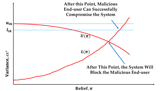
Figure 1: Illustration of a continuous path analysis of $U(\pi)$ and $L(\pi)$ in Markov Perfect Equilibrium

Given this equilibrium concept, our main result is the characterization of querying activity of the malicious end-user and detection (stopping) strategies by the system in a unique equilibrium. We assume that a decision to stop querying (i.e., deviating from honest behavior) is the last action in the game taken by the (malicious) end-user. This decision allows the end-user to either achieve the target of compromising the system and then getting blocked by it or getting blocked without reaching this target at all. In either case, the system’s belief about this end-user will jump to $\pi_{t}=0$. The end-user has no further action, and the game reduces to a straightforward stopping problem for the system i.e., the system decides when to stop the game. In that case, the continuation payoffs from that point on can be interpreted as the termination payoffs of the original signaling game.

Next, consider the state of the game before the end-user deviates/reveals and before the system’s block action. Since malicious end-user plays a mixed strategy that occurs on-equilibrium path, system’s belief about the end-user evolves over time. Thus, a unique MPE consists of a state variable process $(EX_{t}^{v},\pi_{t})$ and two cutoff functions, a non-increasing variance function $U(\pi_{t})$ for the system and an increasing variance function $L(\pi_{t})$ for the end-user, where

• The system immediately blocks the end-user if $ex^{v}_{s_{y},t}\geq U(\pi_{t})$, i.e., $\tau=inf\{t>=0:ex^{v}_{s_{y},t}\geq U(\pi_{t})\}$.

• The malicious end-user keeps querying for explanation (thus, its variance), whenever $ex^{v}_{e_{u},t}<L(\pi_{t})$ and mixes between querying and not querying whenever $ex^{v}_{e_{u},t}\geq L(\pi_{t})$, so that the curve $\{(L(\pi),\pi):\pi\in[0,1]\}$ serves as a reflecting boundary for the process $(ex^{v}_{e_{u},t},\pi_{t})$.

We call such a unique MPE equilibrium a $(U,L)$ equilibrium. The first condition defines an upper boundary which tells the system that if an explanation variance value $ex^{v}_{s_{y},t}$ at time $t$ (corresponding to a query sent by the end-user) is greater than or equal to this boundary ($U(\pi_{t})$), then the end-user is trying to compromise the system. In this case, the system should block the end-user. The second condition above guides the behavior of the malicious end-user. Function $L(\pi_{t})$ represents the upper-bound of the target explanation variance value the malicious end-user wants to achieve given a certain belief $\pi_{t}$ at time $t$. When the explanation variance value corresponding to a query by an end-user is less than this boundary function, i.e., $ex^{v}_{e_{u},t}<L(\pi_{t})$, then it is strategically better for the malicious end-user to keep querying (i.e., looks honest from system’s perspective). However, if $ex^{v}_{e_{u},t}\geq L(\pi_{t})$ then the malicious end-user has an incentive to stop querying. For the malicious end-user, this condition also represents that it is near to the desired (or target) variance threshold value - one more step by the malicious end-user can either lead to success (compromise of the system) or failure (getting blocked by the system before achieving its goal).

For an intuition on the structure of the MPE in our setting, suppose that the current belief is $\pi_{t}$. If the variance computed for an explanation generated by an explanation method is sufficiently large, i.e., close to a threshold variance value, then the system should block the end-user who is suspiciously trying to move in the direction of the model classification boundary. This cutoff for the variance is a non-increasing function of $\pi$ because, by definition, the end-user is less likely to be honest when the variance value is sufficiently close to the threshold value and $\pi_{t}$ is large. Thus, when threshold value becomes greater than or equal to the optimal function $U(\pi_{t})$ at any time $t$, system will block the end-user. This is intuitively shown in Figure 1, where $u_{th}$ represents the variance threshold for an explanation generated by the system and $l_{th}$ represents the variance threshold for the explanation after the system adds noise based on its belief, which can be given to the end-user. [0, $u_{th}]$ or [0, $l_{th}$] represents the pooling region where an MPE can occur, if end-user is not blocked by the system.

4 Equilibrium Analysis

Next, we try to analyze conditions under which a unique MPE exists in the game described above, i.e., we try to construct a $(U,L)$ equilibrium by finding conditions under which optimal functions $L(\pi_{t})$ and $U(\pi_{t})$ exist.

High-level Idea: As mentioned in section 3, an MPE is defined as a pair of functions $L(\pi_{t})$ and $U(\pi_{t})$. Thus, we first need to show that these two optimal functions exists. To prove that $L(\pi_{t})$ and $U(\pi_{t})$ exist, we prove the continuity and differentiability properties of $L(\pi_{t})$ (theorem 1) and $U(\pi_{t})$ (theorem 2) in the belief domain ($\pi_{t}\in[0,1]$). As we have assumed that the system plays a pure strategy, we consider that $U(\pi_{t})$ (for the system) is optimal, and show that it exists and is continuous. However, computing an optimal $L(\pi_{t})$ is non-trivial, as we have assumed that the end-user plays a randomized strategy. Therefore, to compute $L(\pi_{t})$, we first construct two bounding functions $L^{+}(\pi_{t})$ (upper) and $L^{-}(\pi_{t})$ (lower) and show that such functions exists (in lemmas 3 and 4, respectively). To compute these functions we use the boundary conditions (section 2.5) at the decision boundaries, i.e., Pooling, Separating, and Detection and Block (outlined in Table I) and the value functions defined below. We then show that as $\pi_{t}$ increases, $L^{+}(\pi_{t})$ and and $L^{-}(\pi_{t})$ will converge in the range $(0,u_{th})$ (lemma 1) or $(0,l_{th})$ (lemma 2) as we have considered that an MPE occurs when both types of end-user pool. Finally, we show that the first intersection point (root) of $L^{+}(\pi_{t})$ and $L^{-}(\pi_{t})$ is a unique MPE, if the end-user is not blocked by the system before that point. At these decision boundaries, both players decide to either continue or stop.

4.1 Value Functions

As mentioned earlier, we are considering an equilibrium that occurs when both types of end-user pool, i.e., $ex^{v}_{e_{u},t}$ is strictly below $L(\pi_{t})$. In this pooling scenario, no information becomes available to the system about the type of the end-user; thus, belief ($\pi_{t}$) remains constant. Hence, we write the value functions for both the players conditioned on no deviation by the end-user. As we consider an infinite horizon in our game, there is no known terminal (final) value function. Hence, these value functions are independent w.r.t. $t\in R$, as $t$ singularly has no effect on them. The end-user’s value function ($F$) should solve the following HJB equation representing his/her risk-less return:

$$rF(ex^{v}_{e_{u}},\pi)=\mu ex^{v}_{e_{u}}F^{{}^{\prime}}_{ex^{v}_{e_{u}}}(ex^{v}_{e_{u}},\pi)$$

$$+\frac{1}{2}\sigma^{2}(ex^{v}_{e_{u}})^{2}F^{{}^{\prime\prime}}_{ex^{v}_{e_{u}}}(ex^{v}_{e_{u}},\pi)+\psi ex^{v}_{e_{u}}$$

where $F^{{}^{\prime}}_{ex^{v}_{e_{u}}}$ and $F^{{}^{\prime\prime}}_{ex^{v}_{e_{u}}}$ are the first and second order partial derivative of the value function $F(ex^{v}_{e_{u}},\pi)$ w.r.t. $ex^{v}_{e_{u}}$, respectively, and, $\mu$ and $\sigma$ are the drift/mean and the variance/volatility of the variance process $EX_{t}^{v}$, respectively. $\psi$ is the payoff coefficient which depends on the stage payoffs of the end-user, as represented in Table I. The solution to the above equation can be represented as:

$$F(ex^{v}_{e_{u}},\pi)=A_{1}(\pi)(ex^{v}_{e_{u}})^{\beta_{1}}+A_{2}(\pi)(ex^{v}_{e_{u}})^{\beta_{2}}+\frac{\psi ex^{v}_{e_{u}}}{r-\mu}$$

for some constants $A_{1}(\pi)$ and $A_{2}(\pi)$, where $\beta_{1}>1$ and $\beta_{2}<0$ are the roots of the characteristic equation [22]. Similarly, the system’s value function $V(ex^{v}_{s_{y}},\pi)$ should satisfy the following equation, conditioned on $ex^{v}_{e_{u}}<L(\pi)$ and $\pi$ staying constant:

$$rV(ex^{v}_{s_{y}},\pi)=\mu ex^{v}_{s_{y}}V^{{}^{\prime}}_{ex^{v}_{s_{y}}}(ex^{v}_{s_{y}},\pi)$$

$$+\frac{1}{2}\sigma^{2}(ex^{v}_{s_{y}})^{2}V^{{}^{\prime\prime}}_{ex^{v}_{s_{y}}}(ex^{v}_{s_{y}},\pi)+\psi ex^{v}_{s_{y}}$$

where $V^{{}^{\prime}}_{ex^{v}_{s_{y}}}$ and $V^{{}^{\prime\prime}}_{ex^{v}_{s_{y}}}$ are the first and second order partial derivative of the value function $V(ex^{v}_{s_{y}},\pi)$ w.r.t. $ex^{v}_{s_{y}}$, respectively. As before, $\psi$ is the payoff coefficient which depends on the stage payoffs of the system as shown in Table I. The solution to the above equation can be represented as:

$$V(ex^{v}_{s_{y}},\pi)=B_{1}(\pi)\times(ex^{v}_{s_{y}})^{\beta_{1}}+B_{2}(\pi)(ex^{v}_{s_{y}})^{\beta_{2}}+\frac{\psi ex^{v}_{s_{y}}}{r-\mu}$$

for some constant $B_{1}(\pi)$ and $B_{2}(\pi)$. We will use different boundary conditions to determine $A_{1}(\pi)$, $A_{2}(\pi)$, $B_{1}(\pi)$ and $B_{2}(\pi)$. Then, we will use these conditions to determine $U(\pi_{t})$ and $L(\pi_{t})$.

4.2 Analytical Results

Our first aim is to compute the system’s threshold $u_{th}$ (Lemma 1) and the corresponding end-user’s threshold $l_{th}$ (Lemma 2). These thresholds define the region in which an MPE may occur in the game, if the necessary conditions are satisfied. Therefore, these two lemmas will be used to determine if a unique MPE exists in the game or not. Due to space constraints, we have moved all proofs to the supplementary document.

Lemma 1.

There exists a positive upper bound $u_{th}$ on the variance of an explanation generated by an explanation method representing the maximum variance value that can be reached for the query sent by the end-user.

Lemma 2.

There exists a positive upper bound $l_{th}$ on the variance of an explanation given by the system to the end-user representing maximum variance value needed to be reached by the end-user to compromise the system.

Our next aim is to characterize the two optimal cutoff functions, i.e., system’s function $U(\pi_{t})$ and end-user’s function $L(\pi_{t})$, as these two functions represent the MPE in the game. These cut-off functions help the system and the end-user to play optimally in each stage of the game. For example, if the system doesn’t have any knowledge of $U(\pi_{t})$, then it won’t know the range of the variance values being computed for the explanations, which are given to the end-user after adding some noise based on its belief. Hence, an adversary will be able to easily compromise the system. In contrast, $L(\pi_{t})$ function knowledge will guide an adversary on how to optimally compromise the system. For that reason, we first prove that $U(\pi_{t})$ exists and is non-increasing and continuously differentiable (Theorem 1).

Theorem 1.

$U(\pi_{t})$ is non-increasing and continuously differentiable function in domain $[0,1]$ if and only if either $\beta_{2}\beta_{1}J^{`}(\pi,t)^{\beta_{2}-1}\leq\beta_{1}\beta_{2}J^{`}(\pi,t)^{\beta_{1}-1}$ or $\beta_{2}(\beta_{1}-1)J^{`}(\pi,t)^{\beta_{2}-1}\leq\beta_{1}(\beta_{2}-1)J^{`}(\pi,t)^{\beta_{1}-1}$, where $J(\pi,t)=\frac{L(\pi)}{U(\pi)}$.

To prove $L(\pi)$ (Theorem 2) exists and is increasing and continuously differentiable, we first characterize an explanation variance path $L^{+}(\pi)$ (Lemmas 3), which represents the maximum variance values that can be computed by the end-user for the given explanations, and a variance path $L^{-}(\pi)$ (Lemma 4), which represents the minimum variance values for the explanations given by the system to the end-user. We write three equations each for $L^{+}(\pi)$ and $L^{-}(z)$ according to the value matching, smooth pasting, and the condition in which the variance of the explanation received is opposite of what end-user expected. Then, we demonstrate that both these functions are increasing and continuously differentiable. The purpose for doing this is to use these lemmas to show that as $\pi\rightarrow 1$, both $L^{+}(\pi)$ and $L^{-}(\pi)$ starts to converge and becomes equal to $L(\pi)$ after some point.

Lemma 3.

$L^{+}(\pi)$ is a well-defined, increasing, continuous and differentiable function in domain $[0,1]$ if and only if $\lambda^{{}^{\prime}}(L^{+}(\pi),\pi)>0$ and $P>0$, where $\lambda()$ is the termination payoff if the end-user decides to deviate and attack the system.

Lemma 4.

$L^{-}(\pi))$ is a well-defined, increasing, continuous and differentiable function in domain $[0,1]$ if and only if either $(\frac{\partial A_{1}^{+}(z)}{\partial\pi}L^{-}(\pi)^{\beta_{1}}+\frac{\partial A_{2}^{+}(\pi)}{\partial\pi}L^{-}(\pi)^{\beta_{2}})<0$ or $(A_{1}^{+}(\pi)\beta_{1}L^{-}(\pi)^{\beta_{1}-1}+A_{2}^{+}(\pi)\beta_{2}L^{-}(\pi)^{\beta_{2}-1})<0$.

Theorem 2.

$L(\pi)$ is a well-defined, increasing, continuous and differentiable function domain $[0,1]$ if and only if either $\lambda^{{}^{\prime}}(L(\pi),\pi)>0$ and $P>0$.

Finally, we show that such a point where $L^{+}(\pi_{t})$ and $L^{-}(\pi_{t})$ converge (or intersect) exists, and thus, a unique MPE (Theorem 3) exists in the game.

Theorem 3.

A unique MPE or a point, $\varsigma=\frac{\lambda(L^{+}(\pi),\pi)\times(r-\mu)}{P\times L^{-}(\pi)}$, exists in the game where the two curves $L^{+}(\pi)$ and $L^{-}(\pi)$ starts to converge, if and only if $\frac{\beta_{2}}{\varsigma^{\beta_{2}+1}}\left[L^{+}(\lambda^{{}^{\prime}}-\frac{P}{r-\mu})-\beta_{1}(\lambda-\frac{PL^{+}}{r-\mu})\right]\geq\frac{\beta_{1}}{\varsigma^{\beta_{1}+1}}\left[\beta_{2}(\lambda-\frac{PL^{+}}{r-\mu})-L^{+}(\lambda^{{}^{\prime}}-\frac{P}{r-\mu})\right]$.

5 Experimental Setup

We employ the Captum [37] framework to generate four different types of explanations: Gradient*Input, Integrated Gradients, LRP, and Guided Backpropagation. We use PyTorch framework to conduct the training and attack-related experiments. Gradient*Input is used as the baseline (to compare the results of the other explanation methods). Our objective in all the experiments is to analyze and compute the impact of different settings (factors) that can impact the capability of an adversary to launch MIA. We assume that when the game ends, both the system and the end-user will have access to their optimal strategies, thus the optimal explanation variance threshold ($u_{th}$ for the system and $l_{th}$ for the end-user). Hence, an adversary can use its optimal strategy and optimal threshold to conduct MIA, or a system can use its optimal strategy and optimal threshold to protect against MIA. As a result, we focus on two evaluation objectives in our experiments: (i) game evolution, and (ii) MIA accuracy. For the game evolution, we simulate and generate the future explanation variances for $t=100$ stages, according to the expression:

$$EX_{t}^{v}=EX_{0}^{v}*e^{\left((\mu-\frac{1}{2}\sigma^{2})+\sigma W_{t}\right)}\vspace{-0.3cm}$$ (1)

The above equation is the solution to the GBM (Equation 1) of $EX_{t}^{v}$, derived using the it$\hat{o}$’s calculus [22]. $\mu$ and $\sigma>0$ are computed using the variance generated for the test datapoints for each of the dataset. In our experiments, we take $EX_{0}^{v}$ as the last index value of the test data points’ generated explanation variance, as we use this initial value to generate future explanations. Using the obtained optimal strategies and thresholds, we compute the attack accuracy in terms of the attacker’s success rate in launching the MIA or the accuracy of the system in preventing the MIA.

Datasets. We use five popular benchmark datasets on which we perform our game analysis and attack accuracy evaluations: Purchase and Texas datasets [45], CIFAR-10 and CIFAR-100 [51], and the Adult Census dataset [24]. To ease the comparison, the setup and Neural Network (NN) architectures are aligned with existing work on explanation-based threshold attacks [54]. Table II details each dataset’s configuration. Below, we briefly provide details about each of the datasets.

Purchase: This dataset is downloaded from Kaggle’s “Acquire Valued Shoppers Challenge” [2]. The challenge aims to predict customers that will make a repeat purchase. The dataset has $197,324$ customer records, with each record having $600$ binary features. The prediction task is to assign each customer to one of the $100$ labels. We use the same NN architecture used by Shokri et al. [54], a four-layer fully connected neural network with tanh activations and layer sizes equal to $1024$, $512$, $256$ and $100$. We use Adagrad optimizer with a learning rate of $0.01$ and a learning rate decay of $10^{-7}$ to train the model for $50$ epochs.

Texas: This dataset contains patient discharge records from Texas hospitals [1], spanning years 2006 through 2009. It has been used to predict the primary procedures of a patient based on other attributes such as hospital id, gender, length of the stay, diagnosis, etc. This dataset is filtered to incorporate only 100 classes (procedures) and has 67,330 records. The features are transformed to include only binary values, such that each record has 6,170 features. We use a five-layer fully connected NN architecture with tanh activations and layer sizes of 2048, 1024, 512, 256 and 100. We employ the Adagrad optimizer with a learning rate of 0.01 and a learning rate decay of $10^{-7}$ to train the model for 50 epochs.

CIFAR-10 and CIFAR-100: CIFAR-10 and CIFAR-100 are the benchmark datasets for image classification tasks. Each dataset consists of 50K training and 10K test images. As NN architecture, we designed two convolutional layers with max-pooling and two dense layers, all with tanh activations for CIFAR-10 and using Alexnet [38] for CIFAR-100. We train the model for 50 epochs with learning rates of 0.001 and 0.0001 for CIFAR-10 and CIFAR-100, respectively. In both cases, we use Adam optimizer to update the parameters of the model.

Adult: This dataset is downloaded from the 1994 US Census database [24]. It has been used to predict whether a person’s yearly income is above 50,000 USD or not. It has 48,842 records and a total of 14 features, including categorical and numeric features. After transforming categorical features into binary features, each data point resulted in 104 features. A dataset of 5,000 data points is sampled from the original dataset because of the large size, containing 2,500 training data points and 2,500 testing data points. We use a five-layer fully-connected NN architecture with tanh activations and layer sizes equal to 20, 20, 20, 20 and 1. We use an Adagrad optimizer with a learning rate of 0.01 and a learning rate decay of $10^{-7}$ to train the model for 50 epochs.

TABLE II: Dataset Configurations.

Datasets	Points	$\#$Features	Type	$\#$Classes
Purchase	197,324	600	Binary	100
Texas	67,330	6,170	Binary	100
CIFAR-100	60,000	3,072	Image	100
CIFAR-10	60,000	3,072	Image	2
Adult	48,842	24	Mixed	2

Evaluation metric. We compute True Positive Rate (TPR) metric to estimate MIA accuracy after the game has ended and each player has formulated the best response strategy concerning the other player. TPR specifies how accurately an attacker can infer the membership of the data points. We consider training data points to test against the optimal strategy of the system. Since the sample space that we have considered contains only actual training members, there can be only two outcomes: correctly classified and incorrectly classified. The total number of training data points correctly inferred as training points (using $u_{th}$) are called True Positives ($TP$), while the number of training members discerned as non-training members are called False Negatives ($FN$). Thus, $TPR=\frac{TP}{TP+FN}$.

6 Evaluation

In this section, we present experimental analyses of our game model, wherein we compute the impact of different settings on two objectives: (i) the game or equilibrium evolution to obtain optimal strategies and (ii) attack accuracy, i.e., TPR. We begin by analyzing the impact of the Gradient*Input explanations (baseline) on the game equilibrium and attack accuracy for all the considered datasets, and then compare it with the results obtained for the other explanation methods. After that, we also analyze the influence of other factors (e.g., input dimension and overfitting) on the attack accuracy.

6.1 Impact of Different Attack Information Sources

As mentioned in Section 5, for each dataset, we first sample a series of (future) explanations by employing GBM (using Equation 1). The sampled noise is added to the generated explanations variance based on the computed belief at that time (using Bayes’ rule in Section 3.2), such that larger the belief that the end-user is honest, the smaller the noise value added to the explanation, and vice-versa. Then, we compute different functional paths for the system and the end-user defined in Section 3.3 using the closed form representation detailed in Section 4.2, i.e., we compute $U(\pi_{t})$, $L^{+}(\pi_{t})$, $L^{-}(\pi_{t})$ and $L(\pi_{t})$ functions. The termination payoff, $\lambda(ex^{v}_{e_{u}},\pi_{t})$ (defined in 2.5), which is used to write the boundary conditions in the computation of $L^{+}(\pi_{t})$, $L^{-}(\pi_{t})$ and $L(\pi_{t})$ (Lemma 3 and Lemma 4, and Theorem 2) is assumed to be:

$$\lambda(ex^{v}_{e_{u}},\pi_{t})=\frac{0.8\times ex^{v}_{e_{u}}\times log({\pi_{t}\times 2})+\pi_{t}\times ex^{v}_{e_{u}}}{b}$$

where, $ex^{v}_{e_{u}}$ is the value of any end-user’s functional path (considered for the specific computation) at time $t$, and $b$ is the model parameter set differently for each explanation method. The parameters to compute $\lambda(ex^{v}_{e_{u}},\pi_{t})$ are empirically chosen based on their suitability to each of the four explanation methods considered in the paper. Based on our numerical simulations, below are some important observations we make for each dataset, both in the baseline setting (i.e., for the Gradient*Input method) and the other three gradient-based explanation techniques.

(a) CIFAR-10

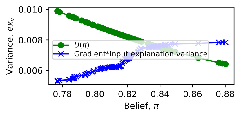
(b) CIFAR-10

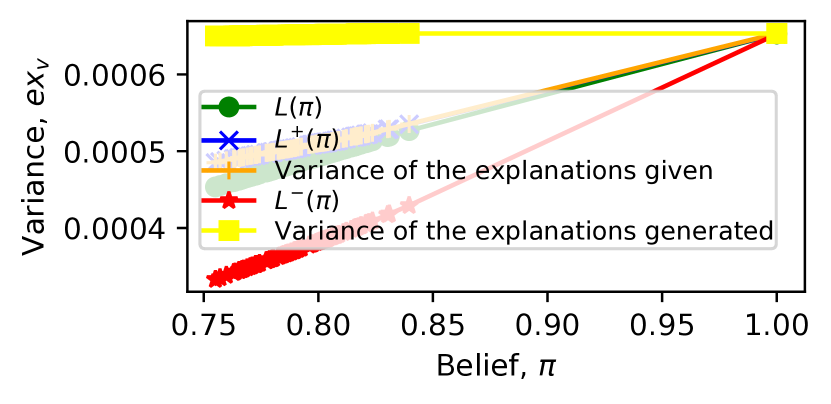
(c) CIFAR-100

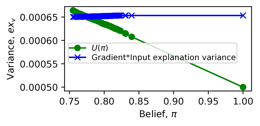
(d) CIFAR-100

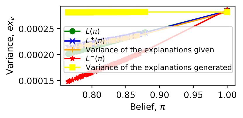
(e) Adult

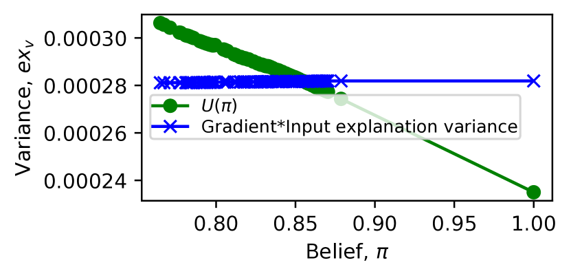
(f) Adult

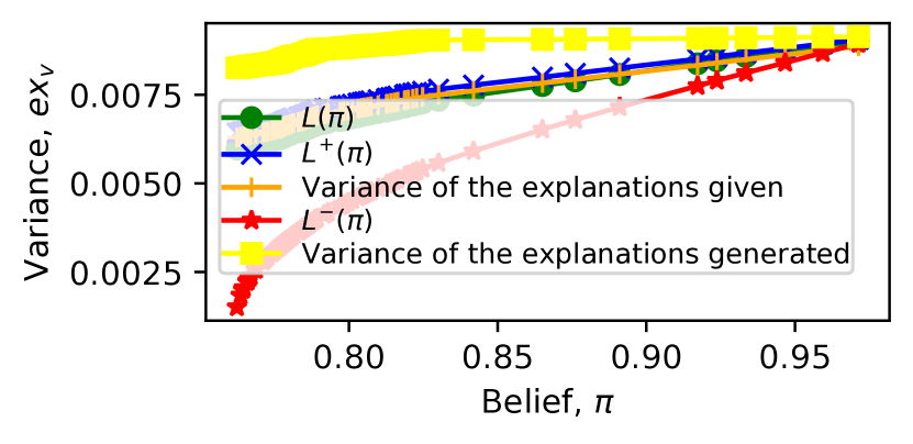
(g) Purchase

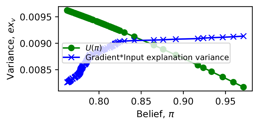
(h) Purchase

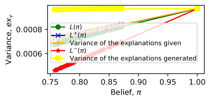
(i) Texas

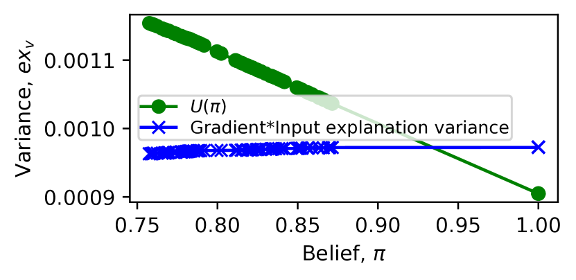
(j) Texas

Figure 2: Different functional paths for the different datasets. (a), (c), (e), (g), and (i) represents the optimal functional paths for the end-user. (b), (d), (f), (h), and (j) represents the optimal functional paths for the system.

Game Evolution in the Baseline Setting: Varying game evolution is realized for different datasets, as shown in Figure 2. Below we analyze in detail the optimal paths obtained for each of the dataset.

• From the plots of the optimal functional path $U(\pi_{t})$ of the system for each of the dataset, as shown in Figures 2(b), 2(d), 2(f), 2(h), and 2(j), we can observe that as $\pi_{t}\rightarrow 1$, $U(\pi_{t})$ starts decreasing. This is because, as the system’s belief about the type of end-user approaches $1$, both the variance of the explanation generated by the system and the variance of the noisy explanation given to the end-user approach $u_{th}$ and $l_{th}$, respectively. After a certain point, i.e., when $ex^{v}_{s_{y}}>U(\pi_{t})$, the system will block the end-user, which confirms to our intuition.

• From the optimal functional paths $L^{+}(\pi_{t})$, $L^{-}(\pi_{t})$ and $L(\pi_{t})$ of the end-user for each of the dataset, as shown in Figures 2(a), 2(c), 2(e), 2(g), and 2(i), we can observe that as $\pi_{t}\rightarrow 1$, $L^{+}(\pi_{t})$, $L^{-}(\pi_{t})$ and $L(\pi_{t})$ approach the threshold $l_{th}$. As discussed in 3.3, as $\pi_{t}\rightarrow 1$ and the variance of the explanation given to the end-user starts to approach the variance threshold, it means a malicious end-user is trying to compromise the system. Thus, if the system doesn’t block the end-user at the right time (or doesn’t have knowledge about optimal $U(\pi)$), then the end-user can easily compromise the system.

• Earlier we showed that a unique MPE exists when $L^{+}(\pi_{t})$ and $L^{-}(\pi_{t})$ begin to converge as $\pi_{t}\rightarrow 1$. This is also visible from our results as shown in Figure 2, where we can observe that as $\pi_{t}\rightarrow 1$, $L^{+}(\pi_{t})$ and $L^{-}(\pi_{t})$ starts to converge. However, for the CIFAR-10 dataset, one can observe that the curves $L^{+}(\pi_{t})$ and $L^{-}(\pi_{t})$ doesn’t converge as $\pi_{t}\rightarrow 1$. Thus, an MPE doesn’t exist in the case of CIFAR-10 dataset. The intuition behind this observation is that the fluctuations (or variance) of the explanation variance computed for the CIFAR-10 is high, making it difficult for them to converge to a single point. Finally, if the system doesn’t block the end-user before the threshold $l_{th}$ or $u_{th}$ is reached, then we say a unique MPE exists in the game.

Attack Accuracy in the Baseline Setting: After obtaining the optimal strategies, we use the range of the training data points of each dataset to determine how many data point variances lie below the computed threshold $u_{th}$ to determine their membership. As shown in Figure 3(a), the attack accuracy for all the datasets except CIFAR-10 is more than 50%. This result aligns with the observed game equilibrium analysis. Hence, the fluctuations in explanation variance make it difficult for an adversary to reach the target threshold, in consequence, to launch MIAs. From these obtained results, one can easily observe that the explanations provide a new opportunity or an attack vector to an adversary actively trying to compromise the system. In other words, our results are clear indicators that an adversary can repeatedly interact with the system to compute the explanation variance threshold and successfully launch membership inference attacks against the system.

Results for other Explanation Techniques: We also analyzed the game for the three other explanation methods considered in this paper. We do not plot the game evolution results in this setting as the plots follow a very similar trend as seen in Figure 2, i.e., game equilibrium was achieved for all the datasets except for the CIFAR-10. We uses the same setting as the baseline setting (mentioned above) to compute attack accuracy for these three explanation methods. We obtained each dataset’s attack accuracy as shown in Figure 3(b). For the Texas and Purchase datasets, 100% accuracy was achieved, i.e., an attacker effectively determines the membership of all the data points used for training the model. However, for the CIFAR-10, the attack accuracy was below 50%, and for the Adult dataset, attack accuracy was above 50% only for the LRP explanation method. The reason is again the high fluctuations in the computed variance for the CIFAR-10 dataset (slightly less for the Adult dataset), thus making it difficult for an adversary to determine the membership of the data points in those datasets. These results clearly indicate that, for different explanation methods, an adversary’s capability to launch MIA attacks will vary and may depend on the variance of the explanations.

(a)

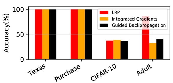
(b)

Figure 3: Accuracy ($TPR$) for the optimal strategy obtained by the system and the end-user: a) Gradient*Input method and b) Other explanation methods.

6.2 Analysis of other Relevant Factors

In this section, we analyze the influence of other factors such as input dimension, underfitting, and overfitting, which can impact the equilibrium evolution, and thus the accuracy of the explanation-based threshold attacks. For this, we analyze the game’s evolution on synthetic datasets and the extent to which an adversary can exploit model gradient information to conduct membership inference attacks. Using artificially generated datasets helps us identify the important factors that can facilitate information leaks.

• Impact of Input dimension. First, we analyze the impact of the input dimension of the data points on the game evolution. To generate datasets, we used the Sklearn make classification module [48]. The number of classes is set to either 2 or 100, while the number of features will vary in range $t_{f}\in[10,100,1000,6000]$. For each setting, we sample 20,000 points and split them evenly into training and test set. Second, for each value $t_{f}$ and for each class, we employ two models to train from this data, namely, model $A$ and model $B$. Model $A$ is chosen to have less layers (or depth) than model $B$; to compare the effect of the complexity of the models on the game evolution and attack accuracy. Model $A$ is a fully connected NN with two hidden layers fifty nodes each, the tanh activation function between the layers, and softmax as the final activation. The network is trained using Adagrad with a learning rate of 0.01 and a learning rate decay of $10^{-7}$ for 50 epochs. Model $B$ is a five-layer fully connected NN with tanh activations. The layer sizes are chosen as 2048, 1024, 512, 256 and 100. We use the Adagrad optimizer with a learning rate of 0.01 and a learning rate decay of $10^{-7}$ to train the model for 50 epochs. Next, we demonstrate the effect of these models on our experiment’s two main objectives.

  • Effect of Model $A$ on Game Evolution and Attack Accuracy. For $k=2$ classes, we observe a similar trend in the game evolution as shown in Figure 2 for each of the features $t_{f}\in[10,100,1000,6000]$. However, for $k=100$ classes, we observed that the belief $\pi_{t}$ of the system about the type of the end-user is always set to $1$ as shown in Figure 4(a). As a consequence, the variance of the explanations generated is equivalent to the variance of the explanations given, as shown in Figure 4(b). Hence, the game didn’t evolve as the system gave the same explanation to the end-user. The reason is because of underfitting. Model $A$ simply does not have enough depth (in terms of the number of layers) to accurately classify 100 classes. Thus, it was not able to accurately classify $100$ classes. Moreover, the loss of model $A$ was approximated to be around $5.74$ for all the features considered, which is not accurate. Hence, the model $A$ gives erroneous results for model predictions. In consequence, it impacts the two objectives of the experiments.

    

    (a)

    

    (b)

    Figure 4: Explanation variance generated vs. explanation variance given when $\pi_{t}=1$.

  • Effect of Model $B$ on Game Evolution and Attack Accuracy. In this case, we considered model $B$ of higher complexity (more layers compared to model $A$) that led to different results compared to model $A$. For $k=2$ classes and $n_{f}=10$, we did not observe any game evolution, because for the test data points explanation variance we got $\sigma>\mu$ and $\sigma>1$. Consequently, the values of the computed future variance of the explanation, using Equation 1, were zero. However, for $t_{f}\in[100,1000,6000]$, we observed the game equilibrium and computed the attack accuracy by sampling from the training data points, as shown in Figure 5(a). For $t_{f}=1000$, an attack accuracy greater than 50% was observed, however, for $t_{f}=100$ and $t_{f}=6000$, an attack accuracy less than 50% was observed. For $k=100$ classes, we did not observe any equilibrium for any of the features $t_{f}$. Therefore, based on the last index value of the explanation variance simulated (i.e. at $t=100$), we computed the threshold $u_{th}$ and accordingly determined the attack accuracy for each of the features as shown in Figure 5(b). In this setting, the loss of the model $B$ was approximated to be around $0.8$ for all the features considered.

  The results obtained for models $A$ and $B$ indicate that the choice of the model used for the classification task on hand also affects the game evolution, and thus, an adversary’s capability to launch MIA attacks against the system.

  

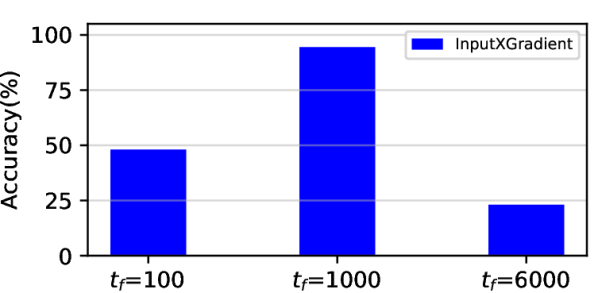
  (a) $k=2$.

  

  (b) $k=100$.

  Figure 5: MIA accuracy for different features $n_{f}$ for model $B$.

• Impact of Overfitting. As detailed in [66], overfitting can significantly increase the accuracy of the membership inference attacks. Thus, to see its effect on the game evolution and attack accuracy in our setup, we varied the number of epochs of the training process. We chose Purchase, Texas, and Adult datasets for this setting. As mentioned in Section 5, the models for these datasets are trained for 50 epochs; thus, to observe the impact of the number of epochs, we trained the models of each dataset for epochs in {30, 50, 60}. The results are shown in Figure 6. We observed that overfitting only increased the attack accuracy for the Adult dataset, while it remained the same for the Texas dataset and decreased for the Purchased dataset. The reason is that the game evolution, and thus the MIA accuracy, depends on multiple factors (mentioned above), hence, the number of training epochs will not singularly determine or impact the capability of an adversary to launch MIA, as presented in the different scenarios mentioned earlier. In other words, the above results show that overfitting does not necessarily increase the attack’s accuracy.

  

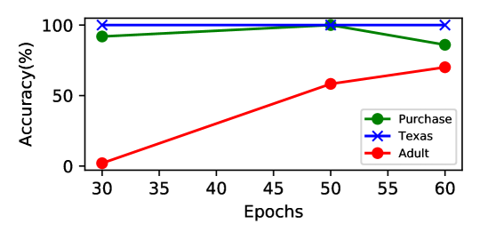
  Figure 6: MIA accuracy for different datasets trained for different epochs.

7 Related Works

In enhancing ML model transparency, privacy concerns have surfaced as a significant challenge. Existing literature highlights the susceptibility of ML models to privacy breaches through various attacks, including membership inference [54], model reconstruction [44, 4], model inversion [67], and sensitive attribute inference attacks [25]. This paper specifically focuses on membership inference attacks or MIAs. MIA attack proposals in the literature can be broadly categorized into three main types based on the construction of the attack model: (i) binary classifier-based, (ii) metric-based, and (iii) differential comparison-based approaches.

• Binary Classifier-based Approaches: Binary classifier-based MIAs involve training a classifier to distinguish the behavior of a target model’s training members from non-members. The widely used shadow training technique [55] is a prominent method, where an attacker creates shadow models to mimic the target model’s behavior. This approach can be categorized as white box or black box, depending on the attacker’s access to the target model’s internal structure [55, 52, 66, 32, 46, 43, 39].

• Metric-based Approaches: Metric-based MIAs simplify the process by calculating certain metrics on prediction vectors and comparing them to a preset threshold to determine the membership status of a data record. Categories within this approach include Prediction Correctness-based MIA [41](determines membership based on correct predictions), Prediction Loss-based MIA [41](infers membership based on prediction loss), Prediction Confidence-based MIA [52](decides membership based on maximum prediction confidence), Prediction Entropy-based MIA [66](uses prediction entropy to infer membership), and Modified Prediction Entropy-based MIA [61](a modification addressing the limitation of existing prediction entropy-based MIA).

• Differential Comparison-based Approaches: In differentially private models [32], where the model preserves user privacy, a novel MIA named BLINDMI is proposed. In this work, BLINDMI generates a non-member dataset by transforming existing samples and differentially moves samples from a target dataset to this generated set iteratively. If the differential move increases the set distance, the sample is considered a non-member, and vice versa.

While existing MIA approaches, such as binary classifier-based and metric-based techniques, have made notable contributions to understanding vulnerabilities in ML models, they come with inherent limitations. Binary classifier-based approaches may rely on assumptions about the adversary’s knowledge of the target model’s structure, potentially limiting their applicability in real-world scenarios where such information is not readily available. Metric-based approaches, while computationally less intensive, often face challenges in determining optimal thresholds for making membership inferences, leading to uncertainties regarding their accuracy. Additionally, these approaches may not provide theoretical guarantees for the optimality of the computed threshold. In contrast, our proposed approach focuses on the mathematical formulation of determining an optimal explanation variance threshold for adversaries to launch MIAs accurately. By addressing the shortcomings of existing methods, our approach aims to offer a theoretically grounded and robust solution, enhancing the security of machine learning models against membership inference attacks.

Consequently, various defenses have been designed to counter MIAs, which fall into four main categories: confidence score masking [65, 55, 40, 36], regularization [30, 52, 46, 17], knowledge distillation [53, 64, 68], and differential privacy [15, 16, 17, 32, 33]. Confidence score masking, utilized in black-box MIAs on classification models, conceals true confidence scores, diminishing the effectiveness of MIAs. Regularization aims to reduce overfitting in target models, with methods such as Logan, ML, and label-based techniques to defend against MIAs. Knowledge distillation involves using a large teacher model to train a smaller student model, transferring knowledge to enhance defense against MIAs. Lastly, differential privacy (DP) is a privacy mechanism that offers an information-theoretical privacy guarantee when training ML models, preventing the learning or retaining of specific user details when the privacy budget is sufficiently small.

While existing defenses against Membership Inference Attacks (MIAs) have made valuable contributions, they have limitations. Although effective against black-box MIAs, confidence score masking may fall short in scenarios where sophisticated adversaries can adapt their strategies. Regularization techniques, while mitigating overfitting, might compromise the model’s performance on the task on which it was trained. Knowledge distillation, reliant on a teacher-student model setup, introduces model architecture and training complexities. Differential privacy, though providing a robust privacy guarantee, often comes at the cost of reduced model utility due to noise injection during training. In contrast, our proposed approach, grounded in a mathematical formulation for the system to determine the optimal explanation variance threshold, aims to address these drawbacks by offering a theoretically sound and adaptable defense mechanism against MIAs.

Game-theoretic approaches, such as zero-sum games [21] [26], non-zero sum games [23], sequential Bayesian games [69] [27], sequential Stackelberg games [14] [5] and simultaneous games [20] have been used in the research literature to model interactions with ML models, specifically to model adversarial classification. Contrary to these efforts, where an adversary’s objective is to target the classification task of an ML model, our research effort focuses on the descriptive task, i.e., explaining the model predictions. Specifically, we use a continuous-time stochastic Signaling Game [47] [13] [8] [60] to model the repeated interactions in a dynamic ML system with explanations to accomplish MIAs. We also make a novel use of GBM [49] [31] [22] to model the explanation variance in order to analyze how an adversary can utilize historical variance information to reach the target variance threshold. To the best of our knowledge, there have been no prior works that utilize a continuous-time game-theoretic formulation to study the privacy leakages (in the form of MIAs) due to model explanations. Similar continuous-time stochastic signaling game models have been used in economic theory to study stock prices [22], dynamic limit pricing [28] [29], and market trading [19]. Our work is one of the first to use modeling concepts from economic theory to study the privacy problem in the ML and model explainability domain.

8 Conclusion

We modeled the strategic interactions between an end-user and a system, where the variance of the explanations generated by the system evolve according to a stochastic differential equation, as a two-player continuous-time signaling game. Our main aim was to study how an adversary can launch explanation-based MIAs by utilizing the explanation variance threshold that he/she computes by repeatedly interacting with the system. In contrast to existing research efforts, this is the first work that analyzes the repeated interaction scenario, in which an adversary builds upon the previously gained knowledge to compute the optimal variance threshold. Our extensive experimental evaluation by considering different gradient-based explanation methods and publicly-available datasets in different settings demonstrates that the capability of an adversary to launch MIA is contingent upon multiple factors, such as the deployed explanation method, datapoint input dimension, model size, and model training rounds. Thus, a shrewd adversary with a working knowledge of all the aforementioned factors can effectively launch MIA by utilizing the information on the variance of the explanations.

8.1 Lemma 1

Proof.

If the variance of the explanation generated by the system reaches $u_{th}$, then system’s belief about the type of end-user becomes zero, i.e., $\pi_{t}=0$, as the end-user’s type is revealed to be malicious. Let’s assume that the system is perfectly able to block the end-user if he/she tries to compromise the system. Hence, using the system’s value function, we get

$$V(u_{th})=\frac{Ku_{th}}{r-\mu}-c_{d}$$ (2)

$$V^{{}^{\prime}}(u_{th})=\frac{K}{r-\mu}$$ (3)

Equation (2) is the value matching condition, which tells that a system will gain $ku_{th}$ while incurring a cost of $-c_{d}$ (detection cost) if it’s able to block the end-user before he/she attacks. Equation (3) is a smooth pasting condition. In Equation (2) and (3), we replace $V(u_{th})$ and it’s derivative $V^{{}^{\prime}}(u_{th})$ with the general solution of the value function of the system and it’s derivative, respectively. As mentioned earlier, at $\pi=0$ the explanation variance given by the system to the end-user becomes zero. As a result, since root $\beta_{2}<0$, second term in the value function can go to $-\infty$. To eliminate this case we make the constant $B_{2}=0$ and we only calculate the constant $B_{1}$.Therefore, equations (2) and (3) are resolved to,

$$B_{1}u_{th}^{\beta_{1}}+\frac{r_{e}u_{th}}{r-\mu}=\frac{ku_{th}}{r-\mu}-c_{d}$$

$$B_{1}\beta_{1}u_{th}^{\beta_{1}-1}+\frac{r_{e}}{r-\mu}=\frac{k}{r-\mu}$$

We first compute the constant $B_{1}$, then find the threshold $u_{th}$. By solving the above two equations using the elimination and substitution method, we get

$$u_{th}=\frac{\beta_{1}c_{d}(r-\mu)}{(\beta_{1}-1)(k-r_{e})}>0$$

As outlined in the payoff assumption, $k>r_{e}$, which implies that $u_{th}>0$. ∎

8.2 Lemma 2

Proof.

It is assumed that if an opportunity arrives for the end-user to compromise the system, then he/she will take one more step after signaling. This step can either make end-user to accomplish his/her’s goal of compromising the system or get’s detected and blocked by it. If end-user gets blocked by the system, the belief will jump to $\pi=0$. Thus, to eliminate the possibility of the second term, $A_{2}l_{th}^{\beta_{2}}\to-\infty$ (as $\beta_{2}<0$) in the general solution of the end-user’s value function, we assume $A_{2}=0$.

Let’s assume that end-user is successful in compromising the system, then the payoff gained by the end-user will be greater than the signaling stage payoff as there will be some monetary benefit to the end-user because of the privacy leak. Using the value matching and the smooth pasting conditions for end-user between signaling and not-signaling stages and accordingly assuming the payoffs received by the end-user, we get

$$A_{1}l_{th}^{\beta_{1}}+\frac{Pl_{th}}{r-\mu}<\frac{M_{NS}^{m}l_{th}}{r-\mu}-d$$ (4)

$$A_{1}\beta_{1}l_{th}^{\beta_{1}-1}+\frac{P}{r-\mu}<\frac{M_{NS}^{m}}{r-\mu}$$ (5)

Solving the above two equations we get,

$$l_{th}>\frac{\beta_{1}d(r-\mu)}{(\beta_{1}-1)(M_{NS}^{m}-P)}>0$$

$M_{NS}^{m}=M^{m}+d^{{}^{\prime}}$, if end-user is successful in compromising the system. Thus, $M_{NS}^{m}>P$, which implies $l_{th}>0$.

∎

8.3 $L^{+}(\pi)$ and $L^{-}(z)$ conditions

Now, we will define the conditions under which an optimal explanation variance path $L(\pi)$ (given optimal $U(\pi)$) exists for the end-user. As mentioned earlier, we are trying to find an MPE in a pooling situation, which will occur when end-user’s explanation lies in the range, $(0,l_{th})$. $l_{th}$ is the explanation variance threshold, which an end-user is trying to achieve to accomplish his/her aim of compromising the system. To find optimal $L(\pi)$, we define two increasing functions, $L^{+}(\pi)$ and $L^{-}(\pi)$. First, we will prove that these two functions exist and then show these two converge by finding out the first intersection point of these two curves as the root of a polynomial (defined below) and finally show that a unique root of that polynomial exists. We will write 3 equations each for $L^{+}(\pi)$ and $L^{-}(z)$ according to the value matching, smooth pasting, and the condition in which the variance of the explanation received is opposite of what end-user expected. That is, if instead of $L^{+}(\pi)$, an end-user gets $L^{-}(\pi)$ or if instead of $L^{-}(\pi)$, an end-user gets $L^{+}(\pi)$ ). Three conditions for $L^{+}(\pi)$ are: -

$$F(L^{+}(\pi),\pi)=\lambda(L^{+}(\pi),\pi)$$

Replacing $F(L^{+}(\pi),\pi)$ with it’s solution, we get

$$A_{1}^{+}(\pi)L^{+}(\pi)^{\beta_{1}}+A_{2}^{+}(\pi)L^{+}(\pi)^{\beta_{2}}$$

$$+\frac{PL^{+}(\pi)}{r-\mu}=\lambda(L^{+}(\pi),\pi)$$ (6)

$$F^{{}^{\prime}}_{L^{+}}(L^{+}(\pi),\pi)=\lambda^{{}^{\prime}}(L^{+}(\pi),\pi)$$

Replacing $F^{{}^{\prime}}_{L^{+}}(L^{+}(\pi),\pi)$ with it’s solution, we get

$$A_{1}^{+}(\pi)\beta_{1}L^{+}(\pi)^{\beta_{1}-1}+A_{2}^{+}(\pi)\beta_{2}L^{+}(\pi)^{\beta_{2}-1}$$

$$+\frac{P}{r-\mu}=\lambda^{{}^{\prime}}(L^{+}(\pi),\pi)$$ (7)

$$F(L^{-}(\pi),\pi)=\frac{P\cdot L^{-}(\pi)}{r-\mu}$$

Replacing $F(L^{-}(\pi),\pi)$ with it’s solution, we get

$$A_{1}^{+}(\pi)L^{-}(\pi)^{\beta_{1}}+A_{2}^{+}(\pi)L^{-}(\pi)^{\beta_{2}}=0$$ (8)

The above conditions are at the boundary between signaling and not-signaling. Equation (6) states that whether successful in compromising the system or not, end-user will get $\lambda(L^{+}(\pi),\pi)$ given the state of the game $(ex,\pi)$. Equation (7) is the smooth pasting condition and equation (8) is when instead of getting $L^{+}(\pi)$, end-user gets $L^{-}(\pi)$. Thus, will receive ($P\cdot L^{-}(\pi)$) from the system.

Three conditions for $L^{-}(\pi)$ are: -

$$F(L^{-}(\pi),\pi)=\frac{PL^{-}(\pi)}{r-\mu}$$

Replacing $F(L^{-}(\pi),\pi)$ with it’s solution, we get

$$A_{1}^{-}(\pi)L^{-}(\pi)^{\beta_{1}}+A_{2}^{-}(\pi)L^{-}(\pi)^{\beta_{2}}=0$$ (9)

$$F^{{}^{\prime}}_{L^{-}}(L^{-}(\pi),\pi)=0$$

Replacing $F^{{}^{\prime}}_{L^{-}}(L^{-}(\pi),\pi)$ with it’s solution, we get

$$A_{1}^{-}(\pi)\beta_{1}L^{-}(\pi)^{\beta_{1}-1}+A_{2}^{-}(\pi)\beta_{2}L^{-}(\pi)^{\beta_{2}-1}=0$$ (10)

$$F(L^{+}(\pi),\pi)=\lambda(L^{+}(\pi),\pi)$$

Replacing $F(L^{+}(\pi),\pi)$ with it’s solution, we get

$$A_{1}^{-}(\pi)L^{+}(\pi)^{\beta_{1}}+A_{2}^{-}(\pi)L^{+}(\pi)^{\beta_{2}}+\frac{PL^{+}(\pi)}{r-\mu}=\lambda(L^{+}(\pi),\pi)$$ (11)

Equation (9) is the value matching condition which states that if the end-user takes one more step, and gets at least the payoff one was getting in the previous stage, then it will stop playing the game. The reason is that $L^{-}(\pi)$ is a value with the highest amount of noise being added to it, hence end-user is already not getting anything. Thus, will want to stop attacking the system. Equation (10) is a smooth pasting condition and equation (11) is when end-user gets $L^{+}(\pi)$ instead of $L^{-}(\pi)$. Thus, there is a chance that end-user can succeed in compromising the system. Hence, getting $\lambda(L^{+}(\pi),\pi)$. The result from these two lemmas will be used in proving the existence and uniqueness of MPE in the game.

8.4 Lemma 3

Proof.

To compute optimal $L^{+}(\pi)$, we assume $\pi$ is set to 1. The reason being, since it’s the variance of an explanation with maximum relevance, the system’s belief about the type of end-user is set to 1. Given belief $\pi=1$, we solve equation (9) and (10) by substitution and elimination approach to get constants $A_{1}^{-}(\pi)$ and $A_{2}^{-}(\pi)$.

We get $A_{1}^{-}(\pi)=0$ and $A_{2}^{-}(\pi)=0$.

Next, using boundary condition (11) and substituting the values of the constants $A_{1}^{-}(\pi)$ and $A_{1}^{-}(\pi)$ in this equation, we get an implicit expression for $L^{+}(\pi)$,

$$\frac{PL^{+}(\pi)}{r-\mu}=\lambda(L^{+}(\pi),\pi)$$

By simplifying the above equation, we get

$$L^{+}(\pi)=\frac{\lambda(L^{+}(\pi),\pi)(r-\mu)}{P}$$ (12)

Taking the derivative of equation 25) we get,

$$\frac{\partial L^{+}(\pi)}{\partial z}=\frac{\lambda^{{}^{\prime}}(L^{+}(\pi),\pi)(r-\mu)}{P}$$ (13)

Since $\lambda^{{}^{\prime}}(L^{+}(\pi),\pi)>0$, $L^{+}(\pi)$ is a well-defined, increasing, continuous and differentiable function. Hence proved.

∎

8.5 Lemma 4

Proof.

Given belief $\pi$, we solve equations (6) and (7) by substitution and elimination approach to get $A_{1}^{+}(\pi)$ and $A_{2}^{+}(\pi)$,

$$A_{1}^{+}(\pi)=\frac{\beta_{2}\lambda(L^{+}(\pi),\pi)-\lambda^{{}^{\prime}}(L^{+}(\pi),\pi)L^{+}(\pi)}{(\beta_{2}-\beta_{1})L^{+}(\pi)^{\beta_{1}}}$$

$$+\frac{P(1-\beta_{2})}{(r-\mu)(\beta_{2}-\beta_{1})L^{+}(\pi)^{\beta_{1}-1}}$$ (14)

$$A_{2}^{+}(\pi)=\frac{\beta_{1}\lambda(L^{+}(\pi),\pi)-\lambda^{{}^{\prime}}(L^{+}(\pi),\pi)L^{+}(\pi)}{(\beta_{1}-\beta_{2})L^{+}(\pi)^{\beta_{2}}}$$

$$+\frac{P(1-\beta_{1})}{(r-\mu)(\beta_{1}-\beta_{2})L^{+}(\pi)^{\beta_{2}-1}}$$ (15)

Now, we will calculate $\frac{\partial A_{1}^{+}(\pi)}{\partial z}$ and $\frac{\partial A_{2}^{+}(\pi)}{\partial z}$ to check for the continuity $A_{1}^{+}(\pi)$ and $A_{2}^{+}(\pi)$ which we will use in checking the continuity of $L^{-}(\pi)$.

$$\frac{\partial A_{1}^{+}(\pi)}{\partial\pi}=\frac{1}{\beta_{2}-\beta_{1}}\times\frac{\partial L^{+}(\pi)}{\partial z}(\frac{\beta_{2}\lambda^{{}^{\prime}}(L^{+}(\pi),\pi)}{L^{+}(\pi)^{\beta_{1}}}$$

$$-\frac{\lambda^{{}^{\prime\prime}}(L^{+}(\pi),\pi)}{L^{+}(\pi)^{\beta_{1}-1}})+\frac{\partial L^{+}(\pi)}{\partial\pi}\times\frac{1}{L^{+}(\pi)}(A_{1}^{+}(\pi)(1-\beta_{1})$$

$$-\frac{\beta_{2}\lambda(L^{+}(\pi),\pi)}{(\beta_{2}-\beta_{1})L^{+}(\pi)^{\beta_{1}}})$$ (16)

$$\frac{\partial A_{2}^{+}(\pi)}{\partial z}=\frac{1}{\beta_{1}-\beta_{2}}\times\frac{\partial L^{+}(\pi)}{\partial z}(\frac{\beta_{1}\lambda^{{}^{\prime}}(L^{+}(\pi),\pi)}{L^{+}(\pi)^{\beta_{2}}}$$

$$-\frac{\lambda^{{}^{\prime\prime}}(L^{+}(\pi),\pi)}{L^{+}(\pi)^{\beta_{2}-1}})+\frac{\partial L^{+}(\pi)}{\partial\pi}\times\frac{1}{L^{+}(\pi)}(A_{1}^{+}(\pi)(1-\beta_{2})$$

$$-\frac{\beta_{1}\lambda(L^{+}(\pi),\pi)}{(\beta_{1}-\beta_{2})L^{+}(\pi)^{\beta_{2}}})$$ (17)

Using boundary condition (8) and taking the derivative of it, gives an implicit expression for $\frac{\partial L^{-}(\pi)}{\partial\pi}$,

$$\frac{\partial A_{1}^{+}(\pi)}{\partial z}L^{-}(\pi)^{\beta_{1}}+\frac{\partial A_{2}^{+}(\pi)}{\partial z}L^{-}(\pi)^{\beta_{2}}$$

$$+A_{1}^{+}(\pi)\beta_{1}L^{-}(\pi)^{\beta_{1}-1}\frac{\partial L^{-}(\pi)}{\partial z}$$

$$+A_{2}^{+}(\pi)\beta_{2}L^{-}(\pi)^{\beta_{2}-1}\frac{\partial L^{-}(\pi)}{\partial\pi}$$ (18)

By simplifying the above equation, we get

$$\frac{\partial L^{-}(\pi)}{\partial\pi}=-\frac{\frac{\partial A_{1}^{+}(\pi)}{\partial\pi}L^{-}(\pi)^{\beta_{1}}+\frac{\partial A_{2}^{+}(\pi)}{\partial\pi}L^{-}(\pi)^{\beta_{2}}}{A_{1}^{+}(\pi)\beta_{1}L^{-}(\pi)^{\beta_{1}-1}+A_{2}^{+}(\pi)\beta_{2}L^{-}(\pi)^{\beta_{2}-1}}$$ (19)

For equation (19) to be greater than zero, either the numerator (represented as $n(L^{-}(\pi))$) or the denominator (represented as $d(L^{-}(\pi))$) has to be negative.

$$n(L^{-}(\pi))=\frac{\partial A_{1}^{+}(z)}{\partial\pi}L^{-}(\pi)^{\beta_{1}}+\frac{\partial A_{2}^{+}(\pi)}{\partial\pi}L^{-}(\pi)^{\beta_{2}}$$ (20)

$$d(L^{-}(\pi))=A_{1}^{+}(\pi)\beta_{1}L^{-}(\pi)^{\beta_{1}-1}+A_{2}^{+}(\pi)\beta_{2}L^{-}(\pi)^{\beta_{2}-1}$$ (21)

Thus, $\frac{\partial L^{-}(\pi)}{\partial\pi}>0$ or $L^{-}(\pi)>0$ if and only if either $n(L^{-}(\pi))<0$ or $d(L^{-}(\pi))<0$.

∎

8.6 Theorem 1

Proof.

We are assuming optimal cutoff function, $U(\pi_{t})$, of the system is optimal as $U(\pi_{t})$ is computed using the belief it has about the type of the end-user. Using three boundary conditions:- value matching, smooth pasting, and instead of $U(\pi_{t})$, the system computes $L(\pi_{t})$ given belief $\pi_{t}$, we calculate the optimal $U(\pi_{t})$. These conditions are assumed at the boundary when the end-user has deviated, and the system has successfully detected the attack. In consequence, account of that end-user is suspended. When system computes $L(\pi_{t})$, which is below $U(\pi_{t})$, it will get a payoff of $r_{e}L(\pi_{t})$. The reason being, since system computes $L(\pi_{t})$, end-user has no incentive to deviate, thus will keep imitating the honest user. As a result, system will get a signaling stage payoff. The three boundary conditions are:

$$V(U(\pi_{t}),z)=\frac{kU(\pi_{t})}{r-\mu}-c_{d}$$

$$V^{{}^{\prime}}_{U}(U(\pi_{t}),\pi)=\frac{k}{r-\mu}$$

$$V(L(\pi_{t}),\pi)=\frac{r_{e}L(\pi_{t})}{r-\mu}$$

By replacing the value of $V(U(\pi_{t}),\pi)$, $V(L(\pi_{t}),\pi)$ and $V^{{}^{\prime}}_{U}(U(\pi_{t}),\pi)$ with the general solution of the value function of the system and it’s derivative, we get the following equations:-

$$B_{1}(\pi)U(\pi_{t})^{\beta_{1}}+B_{2}(z)U(\pi_{t})^{\beta_{2}}+\frac{r_{e}U(\pi_{t})}{r-\mu}=\frac{kU(\pi_{t})}{r-\mu}-c_{d}$$ (22)

$$B_{1}(\pi)\beta U(\pi_{t})^{\beta_{1}-1}+B_{2}(\pi)\beta U(\pi_{t})^{\beta_{2}-1}+\frac{r_{e}}{r-\mu}=\frac{k}{r-\mu}$$ (23)

$$B_{1}(z)L(\pi_{t})^{\beta_{1}}+B_{2}(\pi)L(\pi_{t})^{\beta_{2}}+\frac{r_{e}L(\pi_{t})}{r-\mu}=\frac{r_{e}L(\pi_{t})}{r-\mu}$$ (24)

For simplicity, we will be replacing $L(\pi_{t})$ with $L(\pi)$ and $U(\pi_{t})$ with $U(\pi)$. Solving equations (22) and (23) using substitution and elimination, we get the coefficients $B_{1}$ and $B_{2}$.

$$B_{1}=\frac{(\beta_{2}-1)(k-r_{e})}{(r-\mu)(\beta_{2}-\beta_{1})U(\pi)^{\beta_{1}-1}}-\frac{c_{d}\beta_{2}}{(\beta_{2}-\beta_{1})U(\pi)^{\beta_{1}}}$$

$$B_{2}=\frac{(\beta_{1}-1)(k-r_{e})}{(r-\mu)(\beta_{1}-\beta_{2})U(\pi)^{\beta_{2}-1}}-\frac{c_{d}\beta_{1}}{(\beta_{1}-\beta_{2})U(\pi)^{\beta_{2}}}$$

Now, in order to compute the optimal $U(\pi)$, we substitute the values of $B_{1}$ and $B_{2}$ computed above in equation (24):

$$(\frac{(\beta_{2}-1)(k-r_{e})}{(r-\mu)(\beta_{2}-\beta_{1})U(\pi)^{\beta_{1}-1}}-\frac{c_{d}\beta_{2}}{(\beta_{2}-\beta_{1})U(\pi)^{\beta_{1}}})L(\pi)^{\beta_{1}}$$

$$(\frac{(\beta_{1}-1)(k-r_{e})}{(r-\mu)(\beta_{1}-\beta_{2})U(\pi)^{\beta_{2}-1}}-\frac{c_{d}\beta_{1}}{(\beta_{1}-\beta_{2})U(\pi)^{\beta_{2}}})L(\pi)^{\beta_{2}}=0$$

By simplifying the above equation, we get

$$\frac{(k-r_{e})U(\pi)}{(r-\mu)(\beta_{2}-\beta_{1})}[(\beta_{2}-1)J(\pi,t)^{\beta_{1}}-(\beta_{1}-1)J(\pi,t)^{\beta_{2}}]$$

$$-\frac{c_{d}}{\beta_{2}-\beta_{1}}[\beta_{2}J(\pi,t)^{\beta_{1}}-\beta_{1}J(\pi,t)^{\beta_{2}}]=0$$

$$U(\pi)=\frac{\left[\beta_{2}J(\pi,t)^{\beta_{1}}-\beta_{1}J(\pi,t)^{\beta_{2}}\right]\left(r-\mu\right)}{\left[(\beta_{2}-1)J(\pi,t)^{\beta_{1}}-(\beta_{1}-1)J(\pi,t)^{\beta_{2}}\right]\left(k-r_{e}\right)}$$ (25)

Equation (25) allows us to define a ”best response” threshold curve $U(\pi)$ for the system. We use $J(\pi,t)$ to denote the value of $\frac{L(\pi)}{U(\pi)}$. Now, we will calculate the derivative $\frac{\partial U(\pi)}{\partial\pi}$ to check whether $U(\pi)$ is non-increasing or not. The derivative of $U(\pi)$ depends on it’s numerator (represented as $n(U(\pi))$) and denominator (represented as $d(U(\pi))$) and are given as:

$$n(U(\pi))=\left[\beta_{2}J(\pi,t)^{\beta_{1}}-\beta_{1}J(\pi,t)^{\beta_{2}}\right]\left(r-\mu\right)$$

$$d(U(\pi))=\left[(\beta_{2}-1)J(\pi,t)^{\beta_{1}}-(\beta_{1}-1)J(\pi,t)^{\beta_{2}}\right]\left(k-r_{e}\right)$$

The derivatives of $n(U(\pi))$ and $d(U(\pi))$ are given as:

$$n_{U}(U(\pi))=[\beta_{1}\beta_{2}J^{`}(\pi,t)^{\beta_{1}-1}-\beta_{2}\beta_{1}J^{`}(\pi,t)^{\beta_{2}-1}]\times\left(r-\mu\right)$$ (26)

$$d_{U}(U(\pi))=[\beta_{1}(\beta_{2}-1)J^{`}(\pi,t)^{\beta_{1}-1}-\beta_{2}(\beta_{1}-1)J^{`}(\pi,t)^{\beta_{2}-1}]\times\left(k-r_{e}\right)$$ (27)

Thus, $U(\pi)$ will be non-increasing, if either $n_{U}(U(\pi))<0$ or $d_{U}(U(\pi))<0$.

Checking when $n_{U}(U(\pi))>0$: As we know $\beta_{1}>1$, $\beta_{2}<0$ and $r-\mu>0$. Thus, $n_{U}(U(\pi))>0$ if and only if $\beta_{2}\beta_{1}J^{`}(\pi,t)^{\beta_{2}-1}>\beta_{1}\beta_{2}J^{`}(\pi,t)^{\beta_{1}-1}$ and $n_{U}(U(\pi))<0$ otherwise.

Checking when $d_{U}(U(\pi)>0$: ) We know $k-r_{e}>0$. Thus, $d_{U}(U(\pi))>0$ if and only if $\beta_{2}(\beta_{1}-1)J^{`}(\pi,t)^{\beta_{2}-1}>\beta_{1}(\beta_{2}-1)J^{`}(\pi,t)^{\beta_{1}-1}$ and $n_{U}(U(\pi))<0$ otherwise.

So, $U(\pi)$ will be a non-increasing function if and only if the above conditions are satisfied pertaining to either $n_{U}(U(\pi))<0$ or $d_{U}(U(\pi)<0$.

∎

8.7 Theorem 2

Proof.

Computation of $L(\pi)$ follows the same approach as the computation of $L^{+}(\pi)$, except the belief is not set to 1, i.e., $\pi\neq 1$. The reason being it’s an optimal functional path for the end-user computed at each belief ($\pi$) of the system about the type of the end-user. So, $L(\pi)$ is formulated as:

$$L(\pi)=\frac{\lambda(L(\pi),\pi)(r-\mu)}{P}$$

Taking the derivative of the above equation we get,

$$\frac{\partial L(\pi)}{\partial z}=\frac{\lambda^{{}^{\prime}}(L(\pi),\pi)(r-\mu)}{P}$$

Since $\lambda^{{}^{\prime}}(L(\pi),\pi)>0$ and $P>0$, $L(\pi)$ is a well-defined, increasing, continuous and differentiable function. Hence proved. ∎

8.8 Theorem 3

Proof.

In this proof, first, we will convert the system of equations ((6), (7), (8), (9), (10), (11)) into a system of two equations (shown below). Then, we will try to prove that a unique root exists for this pair of equations. Hence, any solution to this pair of equations will also be a root of the system of equations ((6), (7), (8), (9), (10), (11)). If this root exists and is unique, we say a a unique MPE exists in the game. The pair of equations are derived as follows:

First, we replace the constants in equations (8) and (11), then after rearranging the terms, we get the following two equations:

$$\left[\frac{\beta_{2}\lambda(L^{+}(\pi),\pi)-\lambda^{{}^{\prime}}(L^{+}(\pi),\pi)L^{+}(\pi)}{(\beta_{2}-\beta_{1})}+\frac{P(1-\beta_{2})L^{+}(\pi)}{(r-\mu)(\beta_{2}-\beta_{1})}\right]\times(\frac{1}{\varsigma})^{\beta_{1}}$$

$$+\left[\frac{\beta_{1}\lambda(L^{+}(\pi),\pi)-\lambda^{{}^{\prime}}(L^{+}(\pi),\pi)L^{+}(\pi)}{(\beta_{1}-\beta_{2})}+\frac{P(1-\beta_{1})L^{+}(\pi)}{(r-\mu)(\beta_{1}-\beta_{2})}\right]\times(\frac{1}{\varsigma})^{\beta_{2}}$$ (28)

$$\frac{P\varsigma}{r-\mu}-\frac{\lambda(L^{+}(\pi),\pi)}{L^{-}(\pi)}=0$$ (29)

In the above equations, we have introduced a term $\varsigma$, which is equal to $\frac{L^{+}(\pi)}{L^{-}(\pi)}$ and is a new dependent variable. Thus, any possible root of the above pair of equations will be a value of $\frac{L^{+}(\pi)}{L^{-}(\pi)}$ or of $\varsigma$.

Proof of the existence of $\varsigma$: We will be using concepts from the calculus to prove that a root exists for equations (28) and (29).

From equation (29), we get one of the value of $\varsigma$,

$$\varsigma=\frac{\lambda(L^{+}(\pi),\pi)\times(r-\mu)}{P\times L^{-}(\pi)}$$ (30)

To show that this is the root for the system of equations (28) and (29), we take the curve represented by equation (28) and denote it by $\Lambda$. Then, we will show that only one real root of $\Lambda$ exists in the range $ex\in[0,l_{th}]$, which is the solution to the six boundary conditions.

$$\begin{split}\Lambda(\varsigma)=\left[\frac{\beta_{2}\lambda(L^{+}(z),z)-\lambda^{{}^{\prime}}(L^{+}(z),z)L^{+}(z)}{(\beta_{2}-\beta_{1})}+\frac{P(1-\beta_{2})L^{+}(z)}{(r-\mu)(\beta_{2}-\beta_{1})}\right]\\ \times(\frac{1}{\varsigma})^{\beta_{1}}\\ +\left[\frac{\beta_{1}\lambda(L^{+}(z),z)-\lambda^{{}^{\prime}}(L^{+}(z),z)L^{+}(z)}{(\beta_{1}-\beta_{2})}+\frac{P(1-\beta_{1})L^{+}(z)}{(r-\mu)(\beta_{1}-\beta_{2})}\right]\\ \times(\frac{1}{\varsigma})^{\beta_{2}}\end{split}$$ (31)

The minimum explanation which can be given by the system to the end-user is zero which is at $\pi=0$, thus at this belief, both $L^{-}(\pi)\to 0$ and $L^{+}(\pi)\to 0$. As a result of which, $\varsigma=\frac{0}{0}$. To remove this case, we will assume that $L^{-}(\pi)$ is close to zero, not exactly 0. For the sake of simplicity, let’s denote the coefficient of $(\frac{1}{\varsigma})^{\beta_{1}}$ as $A$ and the coefficient of $(\frac{1}{\varsigma})^{\beta_{2}}$ as $B$ in equation (31). Now, we will check if there exists a root in $ex\in[0,l_{th}]$ or not.

• Case 1: As $ex\to 0$, then $L^{+}(\pi)\to 0$ and $\varsigma\to 0$. As we know $\beta_{1}>1$ and $\beta_{2}<0$, thus $(\frac{1}{\varsigma})^{\beta_{2}}\to 0$ and $(\frac{1}{\varsigma})^{\beta_{1}}\to\infty$. Since we are considering the case when $\pi\to 0$, hence the payoff an end-user gets from the system will be approximately equal to zero. Thus, in the first part of $A$, $\lambda(L^{+}(\pi),\pi)\to 0$ and hence $\lambda^{{}^{\prime}}(L^{+}(\pi)\to 0$. Therefore, $\frac{\beta_{2}\lambda(L^{+}(\pi),\pi)-\lambda^{{}^{\prime}}(L^{+}(\pi),\pi)L^{+}(\pi)}{(\beta_{2}-\beta_{1})}=0$. For the second term of $A$ i.e. $+\frac{P(1-\beta_{2})L^{+}(\pi)}{(r-\mu)(\beta_{2}-\beta_{1})}$, the $numerator>0$ and $denominator<0$. As a result, in this case, $\Lambda(\varsigma)\to-\infty$.

• Case 2: As $ex\to u_{th}$, then $L^{+}(\pi)\to l_{th}$ and $\varsigma\to 1$. If you put these values in equation (19), we will see that $\Lambda(\varsigma)>0$.

Hence, $\Lambda(\varsigma)$ has at-least one root which lies in range $ex\in[0,u_{th}]$.

Proof of uniqueness: Now, we will show that only one root exists for the pair of equations defined above by proving that $\partial\Lambda(\varsigma)$ or $\Lambda_{L^{+}}(\varsigma)$ is increasing in the interval $L^{+}(\pi)\in[0,l_{th}]$ (we could have also taken $L^{-}(\pi)$). Using chain of rule: - $\Lambda_{L^{+}}(\varsigma)$ = $\Lambda_{L^{+}}(\varsigma)$ + $\Lambda_{\varsigma}(\varsigma)\times\varsigma^{{}^{\prime}}$. Hence, $\Lambda(\varsigma)$ will be increasing in the interval or will have a unique root in $[0,l_{th}]$ if $\Lambda_{L^{+}}(\varsigma)>0$ and $\Lambda_{\varsigma}(\varsigma)\times\varsigma^{{}^{\prime}}>0$.

Claim i: For all $ex,\pi$, we have $\Lambda_{L^{+}}(\varsigma)>0$. We have,

$$\begin{split}\Lambda(\varsigma)=\left[\frac{\beta_{2}\lambda(L^{+}(\pi),\pi)-\lambda^{{}^{\prime}}(L^{+}(\pi),\pi)L^{+}(\pi)}{(\beta_{2}-\beta_{1})}+\frac{P(1-\beta_{2})L^{+}(\pi)}{(r-\mu)(\beta_{2}-\beta_{1})}\right]\\ \times(\frac{1}{\varsigma})^{\beta_{1}}+\\ \left[\frac{\beta_{1}\lambda(L^{+}(\pi),\pi)-\lambda^{{}^{\prime}}(L^{+}(\pi),\pi)L^{+}(\pi)}{(\beta_{1}-\beta_{2})}+\frac{P(1-\beta_{1})L^{+}(\pi)}{(r-\mu)(\beta_{1}-\beta_{2})}\right]\\ \times(\frac{1}{\varsigma})^{\beta_{2}}\end{split}$$ (32)

Rearranging the terms will give us:

$$\begin{split}\Lambda(\varsigma)=\frac{1}{\beta_{1}-\beta_{2}}\\ \left[\beta_{1}\lambda(L^{+}(\pi),\pi)-\lambda^{{}^{\prime}}(L^{+}(\pi),\pi)L^{+}(\pi)+\frac{P(1-\beta_{1})L^{+}(\pi)}{(r-\mu)}\right]\\ \times\frac{1}{\varsigma^{\beta_{2}}}-\frac{1}{\beta_{1}-\beta_{2}}\\ \left[\beta_{2}\lambda(L^{+}(\pi),\pi)-\lambda^{{}^{\prime}}(L^{+}(\pi),\pi)L^{+}(\pi)+\frac{P(1-\beta_{2})L^{+}(\pi)}{(r-\mu)}\right]\\ \times\frac{1}{\varsigma^{\beta_{1}}}\end{split}$$ (33)

Now taking derivative of equation (33) with respect to $L^{+}(\pi)$. Taking $L^{+}(\pi)=L^{+}$ and $\lambda(L^{+}(\pi),\pi)=\lambda$ for simplicity.

$$\Lambda_{L^{+}}(\varsigma)=\frac{1}{\beta_{1}-\beta_{2}}\left[\beta_{1}\lambda^{{}^{\prime}}-\lambda^{{}^{\prime\prime}}L^{+}-\lambda^{{}^{\prime}}+\frac{P(1-\beta_{1}}{r-\mu}\right]\times\frac{1}{\varsigma^{\beta_{2}}}$$

$$\frac{1}{\beta_{1}-\beta_{2}}\left[-\beta_{2}\lambda^{{}^{\prime}}+\lambda^{{}^{\prime\prime}}L^{+}+\lambda^{{}^{\prime}}-\frac{P(1-\beta_{2}}{r-\mu}\right]\times\frac{1}{\varsigma^{\beta_{1}}}$$

By rearranging the terms, we get

$$\Lambda_{L^{+}}(\varsigma)=\frac{1}{\beta_{1}-\beta_{2}}\left[(\beta_{1}-1)(\lambda^{{}^{\prime}}-\frac{P}{r-\mu})-\lambda^{{}^{\prime\prime}}L^{+}\right]\times\frac{1}{\varsigma^{\beta_{2}}}$$

$$\frac{1}{\beta_{1}-\beta_{2}}\left[\lambda^{{}^{\prime\prime}}L^{+}+(1-\beta_{2})(\lambda^{{}^{\prime}}-\frac{P}{r-\mu})\right]\times\frac{1}{\varsigma^{\beta_{1}}}$$ (34)

As one can notice, $\lambda^{{}^{\prime}}-\frac{sig}{r-\mu}$ is part of equation (6) or (11), hence positive. Thus, $\Lambda_{L^{+}}(\varsigma)>0$.

Claim ii: For all $ex,\pi$, we have $\Lambda_{\varsigma}(\varsigma)\times\varsigma^{{}^{\prime}}>0$.

We know that $\varsigma=L^{+}(z)/L^{-}(z)$, thus $\varsigma_{L^{+}}>0$.

$$\Lambda_{\varsigma}(\varsigma)=\frac{-\beta_{2}}{\beta_{1}-\beta_{2}}\left[\beta_{1}\lambda-\lambda^{{}^{\prime}}L^{+}+\frac{P(1-\beta_{1})L^{+}}{(r-\mu)}\right]\times\frac{1}{\varsigma^{\beta_{2}+1}}$$

$$-\frac{\beta_{1}}{\beta_{1}-\beta_{2}}\left[\beta_{2}\lambda-\lambda^{{}^{\prime}}L^{+}+\frac{P(1-\beta_{2})L^{+}}{(r-\mu)}\right]\times\frac{1}{\varsigma^{\beta_{1}+1}}$$ (35)

Rearranging equation (35) gives us,

$$\Lambda_{\varsigma}(\varsigma)=\frac{-\beta_{2}}{\beta_{1}-\beta_{2}}\left[\beta_{1}(\lambda-\frac{PL^{+}}{r-\mu})-L^{+}(\lambda^{{}^{\prime}}-\frac{sig}{r-\mu})\right]\times\frac{1}{\varsigma^{\beta_{2}+1}}$$

$$-\frac{\beta_{1}}{\beta_{1}-\beta_{2}}\left[L^{+}(\lambda^{{}^{\prime}}-\frac{sig}{r-\mu})+\beta_{2}(\frac{PL^{+}}{r-\mu}-\lambda)\right]\times\frac{1}{\varsigma^{\beta_{1}+1}}$$ (36)

For $\Lambda_{\varsigma}(\varsigma)>0$, we must have,

$$\frac{\beta_{2}}{\varsigma^{\beta_{2}+1}}\left[L^{+}(\lambda^{{}^{\prime}}-\frac{P}{r-\mu})-\beta_{1}(\lambda-\frac{PL^{+}}{r-\mu})\right]$$

$$\geq\frac{\beta_{1}}{\varsigma^{\beta_{1}+1}}\left[\beta_{2}(\lambda-\frac{PL^{+}}{r-\mu})-L^{+}(\lambda^{{}^{\prime}}-\frac{P}{r-\mu})\right]$$

Hence, if the above condition is true, we will have a unique root of $\Lambda(\varsigma)$which exists in the range $[0,l_{th}]$. Hence proved.

∎

References

- [1] Hospital Discharge Data Public Use Data File. https://www.dshs.texas.gov/THCIC/Hospitals/Download.shtm, 2006. [Online; accessed 11-July-2022].
- [2] Acquire Valued Shoppers Challenge. https://www.kaggle.com/competitions/acquire-valued-shoppers-challenge/overview/description, 2016. [Online; accessed 11-July-2022].
- [3] Muhammad Aurangzeb Ahmad, Carly Eckert, and Ankur Teredesai. Interpretable machine learning in healthcare. In Proceedings of the 2018 ACM international conference on bioinformatics, computational biology, and health informatics, pages 559–560, 2018.
- [4] Ulrich Aïvodji, Alexandre Bolot, and Sébastien Gambs. Model extraction from counterfactual explanations. arXiv preprint arXiv:2009.01884, 2020.
- [5] Scott Alfeld, Xiaojin Zhu, and Paul Barford. Explicit defense actions against test-set attacks. In Thirty-First AAAI Conference on Artificial Intelligence, 2017.
- [6] Marco Ancona, Enea Ceolini, Cengiz Öztireli, and Markus Gross. Towards better understanding of gradient-based attribution methods for deep neural networks. In International Conference on Learning Representations, 2018.
- [7] Leila Arras, Franziska Horn, Grégoire Montavon, Klaus-Robert Müller, and Wojciech Samek. What is relevant in a text document?: An interpretable machine learning approach. PloS one, 12(8):e0181142, 2017.
- [8] Yurii Averboukh. Approximate solutions of continuous-time stochastic games. SIAM Journal on Control and Optimization, 54(5):2629–2649, 2016.
- [9] Microsoft Azure. Model interpretability in Azure Machine Learning (preview). https://docs.microsoft.com/en-us/azure/machine-learning/how-to-machine-learning-interpretability, 2022. [Online; accessed 13-Mar-2022].
- [10] Sebastian Bach, Alexander Binder, Grégoire Montavon, Frederick Klauschen, Klaus-Robert Müller, and Wojciech Samek. On pixel-wise explanations for non-linear classifier decisions by layer-wise relevance propagation. PloS one, 10(7):e0130140, 2015.
- [11] Parth Bhavsar, Ilya Safro, Nidhal Bouaynaya, Robi Polikar, and Dimah Dera. Machine learning in transportation data analytics. In Data analytics for intelligent transportation systems, pages 283–307. Elsevier, 2017.
- [12] Léon Bottou. Large-scale machine learning with stochastic gradient descent. In Proceedings of COMPSTAT’2010, pages 177–186. Springer, 2010.
- [13] Tomás Brázdil, Vojtech Forejt, Jan Krcal, Jan Kretinsky, and Antonin Kucera. Continuous-time stochastic games with time-bounded reachability. In IARCS Annual Conference on Foundations of Software Technology and Theoretical Computer Science. Schloss Dagstuhl-Leibniz-Zentrum fuer Informatik, 2009.
- [14] Michael Brückner and Tobias Scheffer. Stackelberg games for adversarial prediction problems. In Proceedings of the 17th ACM SIGKDD international conference on Knowledge discovery and data mining, pages 547–555, 2011.
- [15] Dingfan Chen, Ning Yu, Yang Zhang, and Mario Fritz. Gan-leaks: A taxonomy of membership inference attacks against generative models. In Proceedings of the 2020 ACM SIGSAC conference on computer and communications security, pages 343–362, 2020.
- [16] Qingrong Chen, Chong Xiang, Minhui Xue, Bo Li, Nikita Borisov, Dali Kaarfar, and Haojin Zhu. Differentially private data generative models. arXiv preprint arXiv:1812.02274, 2018.
- [17] Christopher A Choquette-Choo, Florian Tramer, Nicholas Carlini, and Nicolas Papernot. Label-only membership inference attacks. In International conference on machine learning, pages 1964–1974. PMLR, 2021.
- [18] Google Cloud. Explainable AI: Tools and frameworks to understand and interpret your machine learning models. https://cloud.google.com/explainable-ai, 2022. [Online; accessed 13-Mar-2022].
- [19] Brendan Daley and Brett Green. Waiting for news in the market for lemons. Econometrica, 80(4):1433–1504, 2012.
- [20] Nilesh Dalvi, Pedro Domingos, Sumit Sanghai, and Deepak Verma. Adversarial classification. In Proceedings of the tenth ACM SIGKDD international conference on Knowledge discovery and data mining, pages 99–108, 2004.
- [21] Ofer Dekel, Ohad Shamir, and Lin Xiao. Learning to classify with missing and corrupted features. Machine learning, 81(2):149–178, 2010.
- [22] Robert K Dixit and Robert S Pindyck. Investment under uncertainty. Princeton university press, 2012.
- [23] Lemonia Dritsoula, Patrick Loiseau, and John Musacchio. A game-theoretic analysis of adversarial classification. IEEE Transactions on Information Forensics and Security, 12(12):3094–3109, 2017.
- [24] Dheeru Dua and Casey Graff. UCI machine learning repository, 2017.
- [25] Vasisht Duddu and Antoine Boutet. Inferring sensitive attributes from model explanations. arXiv preprint arXiv:2208.09967, 2022.
- [26] Amir Globerson and Sam Roweis. Nightmare at test time: robust learning by feature deletion. In Proceedings of the 23rd international conference on Machine learning, pages 353–360, 2006.
- [27] Michael Großhans, Christoph Sawade, Michael Brückner, and Tobias Scheffer. Bayesian games for adversarial regression problems. In International Conference on Machine Learning, pages 55–63. PMLR, 2013.
- [28] Sebastian Gryglewicz. Signaling in a stochastic environment and dynamic limit pricing. Technical report, mimeo, Tilburg University, 2009.
- [29] Sebastian Gryglewicz and Aaron Kolb. Strategic pricing in volatile markets. Kelley School of Business Research Paper, (18-28), 2019.
- [30] Jamie Hayes, Luca Melis, George Danezis, and Emiliano De Cristofaro. Logan: Membership inference attacks against generative models. arXiv preprint arXiv:1705.07663, 2017.
- [31] Yaozhong Hu and Bernt Øksendal. Optimal time to invest when the price processes are geometric brownian motions. Finance and Stochastics, 2(3):295–310, 1998.
- [32] Bo Hui, Yuchen Yang, Haolin Yuan, Philippe Burlina, Neil Zhenqiang Gong, and Yinzhi Cao. Practical blind membership inference attack via differential comparisons. arXiv preprint arXiv:2101.01341, 2021.
- [33] Thomas Humphries, Matthew Rafuse, Lindsey Tulloch, Simon Oya, Ian Goldberg, and Florian Kerschbaum. Differentially private learning does not bound membership inference. arXiv preprint arXiv:2010.12112, 2020.
- [34] Alexey Ignatiev, Nina Narodytska, and Joao Marques-Silva. On relating explanations and adversarial examples. Advances in Neural Information Processing Systems, 32:15883–15893, 2019.
- [35] Alon Jacovi, Oren Sar Shalom, and Yoav Goldberg. Understanding convolutional neural networks for text classification. arXiv preprint arXiv:1809.08037, 2018.
- [36] Jinyuan Jia, Ahmed Salem, Michael Backes, Yang Zhang, and Neil Zhenqiang Gong. Memguard: Defending against black-box membership inference attacks via adversarial examples. In Proceedings of the 2019 ACM SIGSAC conference on computer and communications security, pages 259–274, 2019.
- [37] Narine Kokhlikyan, Vivek Miglani, Miguel Martin, Edward Wang, Bilal Alsallakh, Jonathan Reynolds, Alexander Melnikov, Natalia Kliushkina, Carlos Araya, Siqi Yan, et al. Captum: A unified and generic model interpretability library for pytorch. arXiv preprint arXiv:2009.07896, 2020.
- [38] Alex Krizhevsky, Ilya Sutskever, and Geoffrey E Hinton. Imagenet classification with deep convolutional neural networks. Advances in neural information processing systems, 25, 2012.
- [39] Klas Leino and Matt Fredrikson. Stolen memories: Leveraging model memorization for calibrated White-Box membership inference. In 29th USENIX security symposium (USENIX Security 20), pages 1605–1622, 2020.
- [40] Jiacheng Li, Ninghui Li, and Bruno Ribeiro. Membership inference attacks and defenses in classification models. In Proceedings of the Eleventh ACM Conference on Data and Application Security and Privacy, pages 5–16, 2021.
- [41] Yunhui Long, Vincent Bindschaedler, and Carl A Gunter. Towards measuring membership privacy. arXiv preprint arXiv:1712.09136, 2017.
- [42] Scott M Lundberg and Su-In Lee. A unified approach to interpreting model predictions. In Proceedings of the 31st international conference on neural information processing systems, pages 4768–4777, 2017.
- [43] Luca Melis, Congzheng Song, Emiliano De Cristofaro, and Vitaly Shmatikov. Exploiting unintended feature leakage in collaborative learning. In 2019 IEEE symposium on security and privacy (SP), pages 691–706. IEEE, 2019.
- [44] Smitha Milli, Ludwig Schmidt, Anca D Dragan, and Moritz Hardt. Model reconstruction from model explanations. In Proceedings of the Conference on Fairness, Accountability, and Transparency, pages 1–9, 2019.
- [45] Milad Nasr, Reza Shokri, and Amir Houmansadr. Machine learning with membership privacy using adversarial regularization. In Proceedings of the 2018 ACM SIGSAC conference on computer and communications security, pages 634–646, 2018.
- [46] Milad Nasr, Reza Shokri, and Amir Houmansadr. Comprehensive privacy analysis of deep learning: Passive and active white-box inference attacks against centralized and federated learning. In 2019 IEEE symposium on security and privacy (SP), pages 739–753. IEEE, 2019.
- [47] Abraham Neyman. Continuous-time stochastic games. Games and Economic Behavior, 104:92–130, 2017.
- [48] F. Pedregosa, G. Varoquaux, A. Gramfort, V. Michel, B. Thirion, O. Grisel, M. Blondel, P. Prettenhofer, R. Weiss, V. Dubourg, J. Vanderplas, A. Passos, D. Cournapeau, M. Brucher, M. Perrot, and E. Duchesnay. Scikit-learn: Machine learning in Python. Journal of Machine Learning Research, 12:2825–2830, 2011.
- [49] Krishna Reddy and Vaughan Clinton. Simulating stock prices using geometric brownian motion: Evidence from australian companies. Australasian Accounting, Business and Finance Journal, 10(3):23–47, 2016.
- [50] Marco Tulio Ribeiro, Sameer Singh, and Carlos Guestrin. Why should i trust you? explaining the predictions of any classifier. In Proceedings of the 22nd ACM SIGKDD international conference on knowledge discovery and data mining, pages 1135–1144, 2016.
- [51] Alexandre Sablayrolles, Matthijs Douze, Cordelia Schmid, Yann Ollivier, and Hervé Jégou. White-box vs black-box: Bayes optimal strategies for membership inference. In International Conference on Machine Learning, pages 5558–5567. PMLR, 2019.
- [52] Ahmed Salem, Yang Zhang, Mathias Humbert, Pascal Berrang, Mario Fritz, and Michael Backes. Ml-leaks: Model and data independent membership inference attacks and defenses on machine learning models. arXiv preprint arXiv:1806.01246, 2018.
- [53] Virat Shejwalkar and Amir Houmansadr. Membership privacy for machine learning models through knowledge transfer. In Proceedings of the AAAI conference on artificial intelligence, volume 35, pages 9549–9557, 2021.
- [54] Reza Shokri, Martin Strobel, and Yair Zick. On the privacy risks of model explanations. In Proceedings of the 2021 AAAI/ACM Conference on AI, Ethics, and Society, pages 231–241, 2021.
- [55] Reza Shokri, Marco Stronati, Congzheng Song, and Vitaly Shmatikov. Membership inference attacks against machine learning models. In 2017 IEEE symposium on security and privacy (SP), pages 3–18. IEEE, 2017.
- [56] Avanti Shrikumar, Peyton Greenside, and Anshul Kundaje. Learning important features through propagating activation differences. In International Conference on Machine Learning, pages 3145–3153. PMLR, 2017.
- [57] Avanti Shrikumar, Peyton Greenside, Anna Shcherbina, and Anshul Kundaje. Not just a black box: Learning important features through propagating activation differences. arXiv preprint arXiv:1605.01713, 2016.
- [58] Karen Simonyan, Andrea Vedaldi, and Andrew Zisserman. Deep inside convolutional networks: Visualising image classification models and saliency maps. In In Workshop at International Conference on Learning Representations. Citeseer, 2014.
- [59] Dylan Slack, Sophie Hilgard, Emily Jia, Sameer Singh, and Himabindu Lakkaraju. Fooling lime and shap: Adversarial attacks on post hoc explanation methods. In Proceedings of the AAAI/ACM Conference on AI, Ethics, and Society, pages 180–186, 2020.
- [60] Joel Sobel. Signaling games. Complex Social and Behavioral Systems: Game Theory and Agent-Based Models, pages 251–268, 2020.
- [61] Liwei Song and Prateek Mittal. Systematic evaluation of privacy risks of machine learning models. In 30th USENIX Security Symposium (USENIX Security 21), pages 2615–2632, 2021.
- [62] Jost Tobias Springenberg, Alexey Dosovitskiy, Thomas Brox, and Martin Riedmiller. Striving for simplicity: The all convolutional net. arXiv preprint arXiv:1412.6806, 2014.
- [63] Mukund Sundararajan, Ankur Taly, and Qiqi Yan. Axiomatic attribution for deep networks. In International Conference on Machine Learning, pages 3319–3328. PMLR, 2017.
- [64] Xinyu Tang, Saeed Mahloujifar, Liwei Song, Virat Shejwalkar, Milad Nasr, Amir Houmansadr, and Prateek Mittal. Mitigating membership inference attacks by Self-Distillation through a novel ensemble architecture. In 31st USENIX Security Symposium (USENIX Security 22), pages 1433–1450, 2022.
- [65] Ziqi Yang, Bin Shao, Bohan Xuan, Ee-Chien Chang, and Fan Zhang. Defending model inversion and membership inference attacks via prediction purification. arXiv preprint arXiv:2005.03915, 2020.
- [66] Samuel Yeom, Irene Giacomelli, Matt Fredrikson, and Somesh Jha. Privacy risk in machine learning: Analyzing the connection to overfitting. In 2018 IEEE 31st computer security foundations symposium (CSF), pages 268–282. IEEE, 2018.
- [67] Xuejun Zhao, Wencan Zhang, Xiaokui Xiao, and Brian Lim. Exploiting explanations for model inversion attacks. In Proceedings of the IEEE/CVF International Conference on Computer Vision, pages 682–692, 2021.
- [68] Junxiang Zheng, Yongzhi Cao, and Hanpin Wang. Resisting membership inference attacks through knowledge distillation. Neurocomputing, 452:114–126, 2021.
- [69] Yan Zhou and Murat Kantarcioglu. Adversarial learning with bayesian hierarchical mixtures of experts. In Proceedings of the 2014 SIAM International Conference on Data Mining, pages 929–937. SIAM, 2014.