A conservative Eulerian finite element method for transport and diffusion in moving domains

Abstract.

The paper introduces a finite element method for an Eulerian formulation of partial differential equations governing the transport and diffusion of a scalar quantity in a time-dependent domain. The method follows the idea from Lehrenfeld & Olshanskii [ESAIM: M2AN, 53(2): 585-614, 2019] of a solution extension to realise the Eulearian time-stepping scheme. However, a reformulation of the partial differential equation is suggested to derive a scheme which conserves the quantity under consideration exactly on the discrete level. For the spatial discretisation, the paper considers an unfitted finite element method. Ghost-penalty stabilisation is used to release the discrete solution extension and gives a scheme robust against arbitrary intersections between the mesh and geometry interface. The stability is analysed for both first- and second-order backward differentiation formula versions of the scheme. Several numerical examples in two and three spatial dimensions are included to illustrate the potential of this method.

1. Introduction

Mathematical models from biology, chemistry, physics and engineering often include partial differential equations (PDEs) posed on evolving domains. Examples of such problems are fluid flows in or around moving structures such as wind turbines [37] or particle-laden flows [44], biomedical applications such as blood flow through the cardiovascular system [46] or tumour growth [16] and multi-phase flows such as rising bubbles [23] or droplets in microfluidic devices [8].

Computational methods for such problems face the challenge of dealing with both inherently Eulerian quantities, such as concentrations and temperature, and inherently Lagrangian quantities, such as displacements. Many methods that deal with PDEs on evolving domains are based on the Lagrangian or arbitrary Lagrangian–Eulerian (ALE) formulations [22]. Lagrangian and ALE methods can be based on a reference configuration, into which the problem is mapped and in which it is then solved using either standard time-stepping schemes or space-time Galerkin formulations; see, e.g., [45, 30]. An advantage of this approach is that fitted and adapted meshes of the reference geometry can be used, leading to good resolution of the moving interface. However, the approach becomes more limited when the deformation gets large and fails in the case of topology changes. To avoid these issues, purely Eulerian methods can be considered. This will also be our approach.

Within the framework of finite element methods (FEM), unfitted finite element methods have gained traction in the past decade. These include the eXtenden finite element method (XFEM) [14], CutFEM [7], the finite cell method [36] and TraceFEM [33]. These methods are of particular interest in situations of complex geometries, where mesh generation can be a difficult task, as they separate the mesh from the geometry description. As such, they are well suited to moving domain problems, where complex geometries can easily arise. While these methods have been extensively studied for problems on stationary domains, unfitted finite element methods for moving domain problems are less established. One difficulty in the context of evolving domains is due to the approximation of the Eulerian time-derivative

$$\partial_{t}u\approx\frac{1}{\Delta t}(u(t^{n})-u(t^{n-1})).$$

When the domain of interest $\Omega$ changes in time, then $u(t^{n})$ is defined on $\Omega(t^{n})\subset\mathbb{R}^{d}$ and $u(t^{n-1})$ on $\Omega(t^{n-1})$. Consequently, the difference $u(t^{n})-u(t^{n-1})$ may no longer be well-defined.

Several approaches have been developed to try and remedy this problem. These include characteristic-based approaches [18], applying the ALE approach within one time-step and projecting the solution back into the original reference configuration [9] and a Galerkin time-discretisation using modified quadrature rules to recover a classical time-stepping scheme [12]. However, these approaches require expensive projections between domains at different timers. A different and widely studied approach is to use space-time Galerkin approaches [27, 34, 17, 38, 2, 19]. Space-time methods require the solution of $d+1$-dimensional problems and are consequently computationally expensive.

In this work, we will focus on CutFEM as our spatial discretisation. To this end, we consider a static background mesh of our computational domain, and we assume that the volume domain of interest $\Omega(t)$ evolves smoothly within this static computational domain. To handle instabilities arising due to arbitrary ‘cuts’ between $\Omega(t)$ and the background mesh, CutFEM uses ghost-penalty stabilisation [4]. For the temporal discretisation, we modify the Eulerian time-stepping scheme suggested in [26], based on implicit extensions of the solution to a neighbourhood of order $\pazocal{O}(\Delta t)$ using ghost-penalty stabilisation.

The idea of using the extension provided by ghost-penalty stabilisation in CutFEM to enable an Eulerian time-stepping scheme for moving domain problems can be traced back to [42]. However, the method there was limited to a geometric CFL condition $\Delta t\leq c\,h$, as the extension was computed in a separate step. Furthermore, the method was not analysed. The more general method in [26] was then extended and analysed in a number of different settings. In [28], the method was expanded to higher-order geometry approximations using isoparametric mappings. The method was extended to the Stokes problem on moving domains in [5] and [49] using stabilised equal order and Taylor-Hood elements, respectively. In [32], the approach was extended to the linearised Navier-Stokes problem in evolving domains and the a priori error analysis was improved upon. Furthermore, in [48, 47], the approach was analysed for a parabolic model problem for coupled fluid-rigid body interactions. All these approaches were based on a backward differentiation formula (BDF) discretisation of the time-derivative. In [13], the approach has been extended to a Crank-Nicolson discretisation of the time-derivative for the heat-equation on moving domains. However, while the latter study is the first work to extend the approach to non-BDF time-stepping schemes, the analysis required a parabolic CFL condition $\Delta t\leq c\,h^{2}$ not needed for the BDF-type scheme.

In this paper, we revisit the equations governing the conservation of a scalar quantity with a diffusive flux in a domain passively evolved by a smooth flow, as in the original work [26]. While optimal order of convergence with respect to the spatial, temporal- and geometry-approximation was proved in that paper, the method was not optimal in the sense that the conservation of total mass can be violated by the discrete solution. The focus of this work will, therefore, be to develop a modification of this Eulerian time-stepping scheme to preserve the mass of the scalar variable exactly on the discrete level.

The main idea of our approach is to rewrite the PDE problem using an identity derived from the Reynolds transport theorem. Using this identity as the basis of our finite element method, we arrive at a scheme for which we can show that the discrete solution conserves the total mass. The stability analysis presented is similar to that of [26].

The remainder of this paper is structured as follows. In Section 2, we briefly present the PDE problem under consideration, cover the temporally semi-discrete version of our scheme and analyse the unique solvability of the problem and the stability of the scheme. In this semi-discrete setting, the method applies the extension to the test function in the problem formulation, whereas the method in [26] and subsequent works use an extension of the solution into the next domain. In Section 3, we then cover the fully discrete method. We present the fully discrete scheme based on both BDF1 and BDF2 formulas to discretise the time-derivative in the scheme. Furthermore, we consider the discrete stability of both schemes. Finally, in Section 4, we consider a number of numerical examples in two and three spatial dimensions. In examples with a given analytical solution, we investigate the numerical convergence of the schemes with respect to mesh refinement, time-step refinement and combined mesh-time step refinement.

2. Problem setup and preliminaries

Let us consider a time-dependent domain $\Omega(t)\subset\mathbb{R}^{d}$, with $d\in\{2,3\}$, which evolves smoothly and for all time $t\in[0,T]$, $T>0$, stays bounded and embedded in an background fixed domain $\widetilde{\Omega}$, $\Omega(t)\subset\widetilde{\Omega}\subset\mathbb{R}^{d}$. We further assume that the evolution of $\Omega(t)$ is a passive transport by a smooth flow field $\bm{w}\mathrel{\mathop{\mathchar 58\relax}}\widetilde{\Omega}\times(0,T)\to\mathbb{R}^{d}$, i.e. the Lagrangian mapping $\Psi(t)\,\mathrel{\mathop{\mathchar 58\relax}}\,\Omega(0)\to\Omega(t)$ is given by $\Psi(t,y)$ that solves the ODE system

(1) $$\Psi(0,y)=y,\quad\frac{\partial\Psi(t,y)}{\partial t}=\bm{w}(t,\Psi(t,y)),\quad t\in[0,T],\quad y\in\Omega(0),$$

The conservation of a scalar quantity with a diffusive flux in $\Omega(t)$ and no mass exchange through the boundary is governed by the equations

(2a) $$\partial_{t}u+\operatorname{div}(u\bm{w})-\nu\Delta u =f \text{in }\Omega(t),$$

(2b) $$\nabla u\cdot\bm{n} =0 \text{on }\Gamma(t),$$

where $\nu>0$ is a constant diffusion coefficient, $\Gamma(t)\coloneqq\partial\Omega(t)$ is the boundary of the domain, and $\bm{n}$ is the unit normal vector on $\Gamma(t)$. The well-posedness of (2) is addressed, for example, in [1].

The quantity $u$ is globally conserved up to the total contribution of the source term $f$. This is easy to see using Reynolds’ transport formula, equation (2a) and the no-flux boundary condition (2b):

(3) $$\begin{split}\frac{d}{dt}\int_{\Omega(t)}\!\!\!\!u\leavevmode\nobreak\ dx&=\int_{\Omega(t)}\frac{\partial}{\partial t}u\leavevmode\nobreak\ dx+\int_{\partial\Omega(t)}\!\!\!(\bm{w}\cdot\bm{n})u\leavevmode\nobreak\ ds=\int_{\Omega(t)}(\frac{\partial u}{\partial t}+\operatorname{div}(u\bm{w})\,)\leavevmode\nobreak\ dx=\int_{\Omega(t)}\!\!\!\!(\nu\Delta u+f)\,dx\\ &=\int_{\partial\Omega(t)}\!\!\!\!\nu\nabla u\cdot\bm{n}\leavevmode\nobreak\ ds+\int_{\Omega(t)}\!\!\!f\,dx=\int_{\Omega(t)}\!\!\!f\,dx.\end{split}$$

This is a fundamental property, which we would like to preserve in a numerical method.

More generally, for any $v\in H^{1}(\widetilde{\Omega})$ we have

$$\frac{\operatorname{d\!}}{\operatorname{d\!}t}\int_{\Omega(t)}uv\operatorname{d\!}x=\int_{\Omega(t)}\partial_{t}uv\operatorname{d\!}x+\int_{\Gamma(t)}\bm{w}\cdot\bm{n}uv\operatorname{d\!}s=\int_{\Omega(t)}((\partial_{t}u+\operatorname{div}(u\bm{w}))v+u\bm{w}\cdot\nabla v)\operatorname{d\!}x,$$

which follows from Reynolds’ transport formula and the observation that $v$ is time-independent. This yields the identity

(4) $$\int_{\Omega(t)}(\partial_{t}u+\operatorname{div}(u\bm{w}))v\operatorname{d\!}x=\frac{\operatorname{d\!}}{\operatorname{d\!}t}\int_{\Omega(t)}uv\operatorname{d\!}x-\int_{\Omega(t)}u\bm{w}\cdot\nabla v\operatorname{d\!}x.$$

Therefore, multiplying (2a) with a test-function $v\in H^{1}(\widetilde{\Omega})$, integrating by parts and using (2b) and (4) gives the following identity satisfied for a smooth solution to (2) and any $v\in H^{1}(\widetilde{\Omega})$

(5) $$\frac{\operatorname{d\!}}{\operatorname{d\!}t}\int_{\Omega(t)}uv\operatorname{d\!}x+\int_{\Omega(t)}(\nu\nabla u(t)-u(t)\bm{w}(t))\cdot\nabla v\operatorname{d\!}x=\int_{\Omega(t)}f(t)v\operatorname{d\!}x\quad\text{for}\leavevmode\nobreak\ t\in[0,T].$$

This identity will form the basis of our discretisation.

2.1. Temporal semi-discretisation

To elucidate our numerical method construction, we first formulate a semi-discrete method. For this, we need a smooth extension operator

$$\pazocal{E}\mathrel{\mathop{\mathchar 58\relax}}L^{2}(\Omega(t))\rightarrow L^{2}(\widetilde{\Omega}),$$

such that the function remains unchanged in the original domain $\Omega(t)$ and it holds that

$$\|\pazocal{E}u\|_{H^{k}(\widetilde{\Omega})}\lesssim\|u\|_{H^{k}(\Omega(t))}\quad\text{and}\quad\|\nabla\pazocal{E}u\|_{\widetilde{\Omega}}\lesssim\|\nabla u\|_{\Omega(t)}.$$

We refer to [26] for the details of the explicit construction of such an extension operator based on the classical linear and continuous universal extension operator for Sobolev spaces from [43].

Let us consider a uniform time-step $\Delta t=T/N$ for a fixed $N\in\mathbb{N}$. We denote $t_{n}=n\Delta t$, $\Omega^{n}=\Omega(t_{n})$ and $u^{n}\approx u(t^{n})$, and define

$$a^{n}(u,v)\coloneqq\int_{\Omega^{n}}\nu\nabla u\cdot\nabla v-u(\bm{w}^{n}\cdot\nabla v)\operatorname{d\!}x\quad\text{and}\quad f^{n}(v)\coloneqq\int_{\Omega^{n}}f(t^{n})v\operatorname{d\!}x.$$

Using an implicit Euler (or BDF1) discretisation in time of (5) then leads to the problem: Given $u^{n-1}\in H^{1}(\Omega^{n-1})$, find $u^{n}\in H^{1}(\Omega^{n})$ solving

(6) $$\frac{1}{\Delta t}\left[\int_{\Omega^{n}}u^{n}v\operatorname{d\!}x-\int_{\Omega^{n-1}}u^{n-1}\pazocal{E}v\operatorname{d\!}x\right]+a^{n}(u^{n},v)=f^{n}(v),$$

for all $v\in H^{1}(\Omega^{n})$. Note that unlike [26] and subsequent studies, the extension operator in the semi-discrete method acts on the test function rather than on the solution.

In what follow, we shall denote the inner-product for functions in $L^{2}(S)$, for some domain $S$ as $(\cdot,\cdot)_{S}$. Similarly, $\|\cdot\|_{S}$ will denote the $L^{2}(S)$ norm. Furthermore, we use the notation $a\lesssim b$, iff there exists a constant $c>0$, independent of $\delta t$, $h$ and the mesh-interface cut position, such that $a\leq cb$. Similarly, we write $a\gtrsim b$, iff $a\geq cb$, and $a\simeq b$, iff both $a\lesssim b$ and $a\gtrsim b$ hold.

For the bilinear form $a^{n}(\cdot,\cdot)$, we have the following coercivity result.

Lemma 2.1.

Let $w_{\infty}\coloneqq\max_{t\in[0,T]}\|\bm{w}(t)\|_{\infty}$. It holds that

$$a^{n}(u,u)\geq\frac{\nu}{2}\|\nabla u\|_{\Omega^{n}}^{2}-\frac{w_{\infty}^{2}}{\nu}\|u\|_{\Omega^{n}}^{2},$$

i.e., we have unique solvability of the problem (6) in every time-step, if

$$\Delta t<\nu w_{\infty}^{-2}.$$

Proof.

Follows by applying the Cauchy-Schwarz inequality and a weighted Young’s inequality. ∎

It would also be instructive to check the stability of the semi-discrete scheme. We have the following stability result.

Lemma 2.2.

The solution of the semi-discrete scheme in (6), fulfils the stability estimate

$$\|u^{N}\|_{\Omega^{N}}^{2}+\Delta t\sum_{n=1}^{N}\frac{\nu}{4}\|\nabla u^{n}\|_{\Omega^{n}}^{2}\leq\exp(c_{\hyperref@@ii[lemma.smooth-euler.stability]{L\ref*{lemma.smooth-euler.stability}}}T)\left[\|u^{0}\|_{\Omega^{0}}^{2}+\Delta t\sum_{n=1}^{N}\frac{2}{\nu}\|f^{n}\|_{H^{-1}(\Omega^{n})}^{2}\right],$$

with a constant $c_{\hyperref@@ii[lemma.smooth-euler.stability]{L\ref*{lemma.smooth-euler.stability}}}>0$ independent of $\Delta t$, $N$ and $u$, once $\Delta t$ is sufficiently small.

Proof.

Define $\delta$-strip around the moving domain boundary as

$$\pazocal{S}_{\delta}^{\pm}(\Omega(t))\coloneqq\{\bm{x}\in\mathbb{R}^{d}\mathrel{\mathop{\mathchar 58\relax}}\operatorname{dist}(\bm{x},\Gamma(t))\leq\delta\},$$

and the $\delta$-strip outside of the physical domain as

$$\pazocal{S}_{\delta}^{+}(\Omega(t))\coloneqq\pazocal{S}_{\delta}^{\pm}(\Omega(t))\setminus\Omega(t).$$

We choose $\delta\simeq\Delta t$ but sufficiently large such that $\Omega^{n-1}\subset\Omega^{n}\cup\pazocal{S}_{\delta}^{\pm}(\Omega^{n})$ for all $n$. Testing (6) with an appropriate extension of the solution $v=2\Delta t\pazocal{E}u^{n}$ leads to

$$2\|u^{n}\|_{\Omega^{n}}^{2}-\|\pazocal{E}u^{n}\|_{\Omega^{n-1}}^{2}-\|u^{n-1}\|_{\Omega^{n-1}}^{2}+\|\pazocal{E}u^{n}-u^{n-1}\|_{\Omega^{n-1}}^{2}+2\Delta t\nu\|\nabla u^{n}\|_{\Omega^{n}}^{n}-2\Delta t(u^{n},\bm{w}\cdot\nabla u^{n})_{\Omega^{n}}\\ =2\Delta t(f^{n},u^{n})_{\Omega^{n}}.$$

Therefore, using the Cauchy-Schwarz inequalities, we have

$$\|u^{n}\|_{\Omega^{n}}^{2}+\|u^{n}\|_{\Omega^{n}\setminus\Omega^{n-1}}^{2}+\|\pazocal{E}u^{n}-u^{n-1}\|_{\Omega^{n-1}}^{2}+2\Delta t\nu\|\nabla u^{n}\|_{\Omega^{n}}^{2}\\ \leq\|u^{n-1}\|_{\Omega^{n-1}}^{2}+2\Delta t\|f^{n}\|_{H^{-1}(\Omega^{n})}\|\nabla u^{n}\|_{\Omega^{n}}+2\Delta t\sqrt{2}w_{\infty}\|u^{n}\|_{\Omega^{n}}\|\nabla u^{n}\|_{\Omega^{n}}+\|\pazocal{E}u^{n}\|_{\Omega^{n-1}\setminus\Omega^{n}}^{2}.$$

With two weighted Young’s inequalities, we then get

$$\|u^{n}\|_{\Omega^{n}}^{2}+\frac{\Delta t\nu}{2}\|\nabla u^{n}\|_{\Omega^{n}}^{2}\\ \leq\|u^{n-1}\|_{\Omega^{n-1}}^{2}+\frac{2\Delta t}{\nu}\|f^{n}\|_{H^{-1}(\Omega^{n})}^{2}+\frac{4\Delta t}{\nu}w_{\infty}^{2}\|u^{n}\|_{\Omega^{n}}^{2}+\|\pazocal{E}u^{n}\|_{\Omega^{n-1}\setminus\Omega^{n}}^{2}.$$

Since $\Omega^{n-1}\setminus\Omega^{n}\subset\pazocal{S}_{\delta}(\Omega^{n})$, we have the estimate

(7) $$\|\pazocal{E}u^{n}\|_{\Omega^{n-1}\setminus\Omega^{n}}^{2}\leq\|\pazocal{E}u^{n}\|_{\pazocal{S}_{\delta}(\Omega^{n})}^{2}\lesssim(1+\varepsilon^{-1})\delta\|u^{n}\|_{\Omega^{n}}^{2}+\delta\varepsilon\|\nabla u^{n}\|_{\Omega^{n}}^{2},$$

see [26, Lemma 3.5] for the proof of the second estimate. With the choice of $\delta\simeq\Delta t$, we may set $\varepsilon$, such that

$$\|u^{n}\|_{\Omega^{n}}^{2}+\frac{\Delta t\nu}{4}\|\nabla u^{n}\|_{\Omega^{n}}^{2}\\ \leq\|u^{n-1}\|_{\Omega^{n-1}}^{2}+\frac{2\Delta t}{\nu}\|f^{n}\|_{H^{-1}(\Omega^{n})}^{2}+\Delta t\left(\frac{4w_{\infty}}{\nu}+c(\nu^{-1})\right)\|u^{n}\|_{\Omega^{n}}^{2}.$$

Summing over $n=1,\dots,N$ and applying a discrete Grönwall’s estimate, c.f. [21], for $\Delta t$ sufficiently small such that $\Delta t\big{(}4w_{\infty}\nu^{-1}+c(\nu^{-1})\big{)}<1$, gives the result. ∎

3. Discrete Method

We now formulate a fully discrete counterpart to (6). For the spatial discretisation, we use unfitted finite element, also known as CutFEM [7]. We consider a quasi-uniform simplicial mesh $\pazocal{T}_{h}$ of $\widetilde{\Omega}$ with characteristic element diameter $h>0$. Thus the mesh is independent of $\Omega(t)$. On this background mesh, we define the finite element space

$$V_{h}\coloneqq\{v\in C(\widetilde{\Omega})\mathrel{\mathop{\mathchar 58\relax}}{\left.\kern-1.2ptv\right|_{K}}\in\mathbb{P}^{k}(K),\text{ for all }K\in\pazocal{T}_{h}\},\quad k\geq 1,$$

where $\mathbb{P}^{k}(K)$ is space of polynomials of order $k$ on $K$. In each time step, the domain $\Omega^{n}$ is approximated by $\Omega_{h}^{n}$, which is computed by an approximated level set function, see Section 3.2 below. For a the discrete formulation, we now consider at each time step $\delta_{h}$-extensions of the discrete domains:

(8) $$\pazocal{O}_{\delta_{h}}(\Omega_{h}^{n})\mathrel{\mathop{\mathchar 58\relax}}=\{\bm{x}\in\widetilde{\Omega}\,\mathrel{\mathop{\mathchar 58\relax}}\,\mbox{dist}(\bm{x},\Omega_{h}^{n})<\delta_{h}\},\quad\delta_{h}=c_{\delta}w_{\bm{n}}^{\infty}\Delta t,$$

with some $c_{\delta}\simeq 1$ defined later. Using this extension, we define the active mesh in each time step as the set of elements with some part in the extended domain

$$\pazocal{T}_{h}^{n}\coloneqq\{K\in\pazocal{T}_{h}\mathrel{\mathop{\mathchar 58\relax}}\operatorname{dist}(\bm{x},\Omega_{h}^{n})\leq\delta_{h},\;\bm{x}\in K\}.$$

Consequently, we define the active domain as

$$\widetilde{\Omega}^{n}_{h}=\{\bm{x}\in\overline{K}\mathrel{\mathop{\mathchar 58\relax}}K\in\pazocal{T}_{h}^{n}\}.$$

A sketch of this can be seen in Figure 1. With above choice (8), we then have the essential property for our method, that

$$\Omega^{n-1}_{h}\subset\widetilde{\Omega}^{n}_{h}.$$

Finally, in each time step, we then take the restriction of the finite element space to the set of active elements

$$V_{h}^{n}\coloneqq\{v\in C(\widetilde{\Omega})\mathrel{\mathop{\mathchar 58\relax}}{\left.\kern-1.2ptv\right|_{K}}\in\mathbb{P}^{k}(T),\text{ for all }K\in\pazocal{T}_{h}^{n}\}.$$

Figure 1. Sketch of the different sets of elements and facets used in the discrete method.

3.1. Finite element formulation

To formulate the discrete problem, let us define the (bi-) linear forms

$$a_{h}^{n}(u,v)=\int_{\Omega_{h}^{n}}\nu\nabla u\cdot\nabla v-u(\bm{w}^{n}\cdot\nabla v)\operatorname{d\!}x,\quad\text{and}\quad f_{h}^{n}(v)=\int_{\Omega_{h}^{n}}f^{n}v\operatorname{d\!}x.$$

Furthermore, let $s_{h}^{n}(u,v)$ be a stabilisation bilinear form which acts in a strip $\pazocal{S}_{\delta_{h}}^{\pm}$ around $\Omega_{h}^{n}$, such that $\Omega_{h}^{n+1}\subset\Omega_{h}^{n}\cup\widetilde{\Omega}^{n}_{h}$. In practice, this is a ghost-penalty operator, see Section 3.1.2 below.

Using an implicit Euler discretisation of the time-derivative, the fully discrete scheme then reads as follows: Given $u^{0}$, find $u_{h}^{n}\in V_{h}^{n}$, for $n=1,\dots,N$, such that

(9) $$\frac{1}{\Delta t}\left[\int_{\Omega_{h}^{n}}u_{h}^{n}v_{h}\operatorname{d\!}x-\int_{\Omega_{h}^{n-1}}u_{h}^{n-1}v_{h}\operatorname{d\!}x\right]+a_{h}^{n}(u_{h}^{n},v_{h})+\nu s_{h}^{n}(u_{h}^{n},v_{h})=f_{h}^{n}(v_{h}),$$

for all $v_{h}\in V_{h}^{n}$.

Remark 3.1 (Conservation).

The scheme presented in (9) is conservative, if the stabilisation term vanishes for constant test functions. Testing with $v_{h}\equiv 1$, for which $a_{h}^{n}$ and the ghost-penalty term vanishes and summing gives

$$\int_{\Omega_{h}^{n}}u_{h}^{n}\operatorname{d\!}x=\int_{\Omega_{h}^{0}}u_{h}^{0}\operatorname{d\!}x+\Delta t\sum_{k=1}^{n}\int_{\Omega_{h}^{k}}f^{k}\operatorname{d\!}x,$$

which is the discrete counterpart of (3).

3.1.1. Higher order in time

A simple extension of the above method is to use a second-order backward-differentiation formula (BDF2) for the time derivative. This then reads as follows: Given $u^{0}$, compute $u_{h}^{1}$ using (9) and find $u_{h}^{n}\in V_{h}^{n}$, for $n=2,\dots,N$, such that

(10) $$\frac{1}{\Delta t}\left[\frac{3}{2}\int_{\Omega_{h}^{n}}u_{h}^{n}v_{h}\operatorname{d\!}x-2\int_{\Omega_{h}^{n-1}}u_{h}^{n-1}v_{h}\operatorname{d\!}x+\frac{1}{2}\int_{\Omega_{h}^{n-2}}u_{h}^{n-2}v_{h}\operatorname{d\!}x\right]+a_{h}^{n}(u_{h}^{n},v_{h})+\nu s_{h}^{n}(u_{h}^{n},v_{h})=f_{h}^{n}(v_{h}),$$

for all $v_{h}\in V_{h}$. By increasing the width of the extension strip to by a factor of two in (8), this is then well posed.

Remark 3.2.

Same as (9), the BDF2 scheme conserves the scalar quantity, up to forcing terms.

3.1.2. Stabilising bilinear form

In problem (9), the extension into the active domain is realised through the stabilising form $s_{h}^{n}(\cdot,\cdot)$. We shall take $s_{h}^{n}$ to be a ghost-penalty stabilisation operator [4]. The original aim for this kind of stabilisation is to prevent stability and conditioning problems occurring in unfitted finite elements in the presence of so-called bad cuts, i.e., elements where $|K\cap\Omega|$ is very small, by giving a stable solution on the whole of each cut element. Ghost-penalty stabilisation additionally provides us with an implicitly extended solution outside of the physical domain. By applying this stabilisation in a strip around $\Gamma^{n}_{h}$, as first proposed in [26], we obtain the necessary discrete extension for our Eulerian time-stepping scheme. To this end, we define the set of boundary strip elements as

$$\pazocal{T}_{\pazocal{S}^{\pm}_{\delta}}^{n}\coloneqq\{K\in\pazocal{T}_{h}^{n}\mathrel{\mathop{\mathchar 58\relax}}\operatorname{dist}(\bm{x},\Gamma^{n}_{h})\leq\delta_{h},\;\bm{x}\in K\},$$

and the set of facets of these elements, that are interior to the active mesh

$$\pazocal{F}_{h}^{n}\coloneqq\{F=\overline{K}_{1}\cap\overline{K}_{2}\mathrel{\mathop{\mathchar 58\relax}}K_{1}\in\pazocal{T}_{\pazocal{S}^{\pm}_{\delta}}^{n},K_{2}\in\pazocal{T}_{h}^{n},K_{1}\neq K_{2},\operatorname{meas}_{d-1}(F)>0\}.$$

A number of different versions of the ghost-penalty operator exist, the most common version being based on normal derivative jumps across relevant facets, see for example [5, 6, 11, 13, 29]. We prefer the so-called direct-version, introduced in [38], since this extends more easily to higher-order spaces. For a more detailed overview, we refer to [26, Section 4.3].

To define the direct ghost-penalty operator, let $\pazocal{E}^{\mathbb{P}}\colon\mathbb{P}^{k}(K)\rightarrow\mathbb{P}^{k}(\mathbb{R}^{d})$ be the canonical global extension operator of polynomials to $\mathbb{R}^{d}$, i.e., for $v\in\mathbb{P}^{k}(K)$ it holds that ${\left.\kern-1.2pt\pazocal{E}^{\mathbb{P}}(v)\right|_{K}}=v$. For a facet $F=\overline{K}_{1}\cap\overline{K}_{2}$, $K_{1}\neq K_{2}$, we define the facet patch as $\omega_{F}=\operatorname{Int}(\overline{K}_{1}\cup\overline{K}_{2})$. The volumetric patch jump of a polynomial $v_{h}\in\mathbb{P}^{k}(\pazocal{T}_{h})$ is then defined via

$${\left.\kern-1.2pt\llbracket v_{h}\rrbracket\right|_{K_{1}}}={\left.\kern-1.2ptv_{h}\right|_{K_{i}}}-\pazocal{E}^{\mathbb{P}}({\left.\kern-1.2ptv_{h}\right|_{K_{j}}}),\quad\text{for }i,j\in\{1,2\}\text{ and }i\neq j.$$

The direct version of the ghost-penalty operator is then defined as

$$s_{h}^{n}(u_{h},v_{h})\coloneqq\gamma_{s}\sum_{F\in\pazocal{F}_{h}^{n}}\frac{1}{h^{2}}\int_{\omega_{F}}\llbracket u_{h}\rrbracket\llbracket v_{h}\rrbracket\operatorname{d\!}x,$$

with a stabilisation parameter $\gamma_{s}>0$. For this operator to provide the necessary stability, the stability parameter needs to scale with number of facets which need to be crossed to reach an element interior to the physical domain from an element in the extension strip [26]. This number $L$ depends on the anisotropy between the mesh size and time-step by $L\lesssim(1+\delta_{h}/h)\simeq(1+c\Delta t/h)$. Accordingly, we set

$$\gamma_{s}=c_{\gamma}L,\quad\text{with }c_{\gamma}>0\text{ independent of $h$ and $\Delta t$}.$$

See also [26] for further details to this choice.

Assumption 3.3.

For every element $K\in\pazocal{T}_{\pazocal{S}^{+}_{\delta}}^{n}$, there exists an uncut element $K^{\prime}\in\pazocal{T}_{\pazocal{S}^{\pm}_{\delta}}^{n}\setminus\pazocal{T}_{\pazocal{S}^{+}_{\delta}}^{n}$, which can be reached by repeatedly crossing facets in $\pazocal{F}_{h}^{n}$. We assume that the number of facets that must be crossed to reach $K$ from $K^{\prime}$ is bounded by a constant $L\lesssim 1+\frac{\delta_{h}}{h}$. Furthermore, we assume that each uncut element $K^{\prime}\in\pazocal{T}_{\pazocal{S}^{\pm}_{\delta}}^{n}\setminus\pazocal{T}_{\pazocal{S}^{+}_{\delta}}^{n}$ is the end of at most $M$ such paths, with $M$ bounded independent of $h$ and $\Delta t$.

The key result for the ghost-penalty operator is the following ghost-penalty mechanism.

Lemma 3.4.

Under 3.3, it holds for $u_{h}\in V_{h}^{n}$ that

(11) $$c_{\hyperref@@ii[lem:gp-mechanism]{L\ref*{lem:gp-mechanism}a}}\left(\|\nabla u_{h}\|_{\Omega_{h}^{n}}+s_{h}^{n}(u_{h},u_{h})\right)\leq\|\nabla u_{h}\|_{\widetilde{\Omega}^{n}_{h}}^{2}\leq c_{\hyperref@@ii[lem:gp-mechanism]{L\ref*{lem:gp-mechanism}b}}\left(\|\nabla u_{h}\|_{\Omega_{h}^{n}}+s_{h}^{n}(u_{h},u_{h})\right),$$

with constants $c_{\hyperref@@ii[lem:gp-mechanism]{L\ref*{lem:gp-mechanism}a}},c_{\hyperref@@ii[lem:gp-mechanism]{L\ref*{lem:gp-mechanism}b}}>0$ independent of the mesh size and mesh-interface cut configuration.

See [26, Lemma 5.5] for a proof thereof.

Remark 3.5.

Note that we can choose a smaller, necessary, set of facets for the ghost-penalty stabilisation form, to avoid couplings between all elements with a facet in $\pazocal{F}_{h}^{n}$, considered for example in [3, 20]. However, we keep the above, sufficient, set $\pazocal{F}_{h}^{n}$ here for simplicity.

3.2. Geometry description

We assume that the discrete geometry $\Omega_{h}^{n}$ is represented by a discrete level set function. That is,

$$\Omega_{h}^{n}\coloneqq\{\bm{x}\in\mathbb{R}^{d}\mathrel{\mathop{\mathchar 58\relax}}\phi_{h}(\bm{x},t^{n})\leq 0\},$$

where $\phi_{h}$ is a piecewise-linear interpolation of a smooth level set function $\phi$. See also [7, Section 4] for further details of geometry descriptions in CutFEM. The piecewise linear level set approximation introduces a geometry approximation error of order $h^{2}$. However, we will only consider piecewise-linear finite elements, i.e., $k=1$; consequently, second-order convergence is optimal. Higher-order geometry approximations for level set geometries can be achieved in a number of different methods, see, e.g., [24, 15, 31, 35, 39]. In particular, the isoparametric approach [24] has also been analysed in the Eulerian moving domain setting [28]. We note that because our method evaluates every $u_{h}^{n}$ only on $\Omega_{h}^{n}$, we expect the isoparametric geometry approximation analysis for this method to be significantly simpler than in [28], where functions defined with respect to a mesh deformation have to be evaluated accurately on a mesh with a different deformation.

3.3. Stability

Using the ghost-penalty mechanism, we obtain a similar stability result as for the temporally semi-discrete scheme.

Lemma 3.6 (Discrete stability for BDF1).

The solution of the finite element method (9), we have for sufficiently small $\Delta t$ and $h^{2}$, the stability estimate

$$\|u_{h}^{N}\|_{\Omega_{h}^{N}}^{2}+\Delta t\sum_{n=1}^{N}\frac{\nu}{2c_{\hyperref@@ii[lem:gp-mechanism]{L\ref*{lem:gp-mechanism}b}}}\|\nabla u_{h}^{n}\|_{\widetilde{\Omega}^{n}_{h}}^{2}\leq\exp(c_{\hyperref@@ii[lem:stability.discrete.bdf1]{L\ref*{lem:stability.discrete.bdf1}}}T)\left(\|u_{h}^{0}\|_{\Omega_{h}^{0}}^{2}+\Delta t\sum_{n=1}^{N}\frac{2}{\nu}\|f_{h}^{n}\|_{H^{-1}(\Omega_{h}^{n})}^{2}\right),$$

with a constant $c_{\hyperref@@ii[lem:stability.discrete.bdf1]{L\ref*{lem:stability.discrete.bdf1}}}$ independent of $h$, $\Delta t$, $N$ and the mesh-interface cut configurations.

Proof.

Testing (9) with $v_{h}=2\Delta tu_{h}^{n}$ gives

$$2\|u_{h}^{n}\|_{\Omega_{h}^{n}}^{2}-2(u_{h}^{n-1},u_{h}^{n})_{\Omega_{h}^{n-1}}+2\nu\Delta t\|\nabla u_{h}^{n}\|_{\Omega_{h}^{n}}^{2}-2\Delta t(u_{h}^{n},\bm{w}^{n}\cdot\nabla u_{h}^{n})_{\Omega_{h}^{n}}+2\Delta ts_{h}^{n}(u_{h}^{n},u_{h}^{n})=2\Delta t(f_{h}^{n},u_{h}^{n})_{\Omega_{h}^{n}}.$$

Using the Cauchy-Schwarz and weighted Young’s inequality, dropping positive term on the left-hand side and using the ghost-penalty mechanism (11), we get

(12) $$\|u_{h}^{n}\|_{\Omega_{h}^{n}}^{2}+\frac{\nu\Delta t}{c_{\hyperref@@ii[lem:gp-mechanism]{L\ref*{lem:gp-mechanism}b}}}\|\nabla u_{h}^{n}\|_{\widetilde{\Omega}^{n}_{h}}^{2}\leq\|u_{h}^{n-1}\|_{\Omega_{h}^{n-1}}^{2}+\frac{2\Delta t}{\nu}\|f_{h}^{n}\|_{H^{-1}(\Omega_{h}^{n})}^{2}+\frac{4\Delta t}{\nu}w_{\infty}^{2}\|u_{h}^{n}\|_{\Omega_{h}^{n}}^{2}+\|u_{h}^{n}\|_{\Omega_{h}^{n-1}\setminus\Omega_{h}^{n}}^{2}$$

To bound the solution on the extension strip, we use a discrete version of (7). In particular, it holds under 3.3, that for all $u_{h}\in V_{h}^{n}$ and any $\varepsilon>0$

(13) $$c_{1}\|u_{h}\|_{\pazocal{S}_{\delta_{h}}^{+}(\Omega_{h}^{n})}^{2}\leq\delta_{h}(1+\varepsilon^{-1})\|u_{h}\|_{\Omega_{h}^{n}}^{2}+\delta_{h}\varepsilon\|\nabla u_{h}\|_{\Omega_{h}^{n}}^{2}+\delta_{h}L((1+\varepsilon^{-1})h^{2}+\varepsilon)s_{h}^{n}(u_{h},u_{h}),$$

with $c_{1}>0$ independent of $h$ and mesh-interface cut configuration, see [26, Lemma 5.7]. With the choice of $\varepsilon<\nu c_{1}(2c_{\delta_{h}}w_{\bm{n}}^{\infty}c_{\hyperref@@ii[lem:gp-mechanism]{L\ref*{lem:gp-mechanism}b}})^{-1}$ and $h^{2}$ sufficiently small, we have

$$\|u_{h}^{n}\|_{\Omega_{h}^{n-1}\setminus\Omega_{h}^{n}}^{2}\leq\|u_{h}^{n}\|_{\pazocal{S}_{\delta_{h}}^{+}(\Omega_{h}^{n})}^{2}\leq c_{2}\Delta t\|u_{h}^{n}\|_{\Omega_{h}^{n}}+\frac{\nu\Delta t}{2c_{\hyperref@@ii[lem:gp-mechanism]{L\ref*{lem:gp-mechanism}b}}}\|\nabla u_{h}^{n}\|_{\widetilde{\Omega}^{n}_{h}}^{2},$$

with $c_{2}>0$ independent of $h$ and mesh-interface cut configuration. Inserting this in (12) then gives

(14) $$\|u_{h}^{n}\|_{\Omega_{h}^{n}}^{2}+\frac{\nu\Delta t}{2c_{\hyperref@@ii[lem:gp-mechanism]{L\ref*{lem:gp-mechanism}b}}}\|\nabla u_{h}^{n}\|_{\widetilde{\Omega}^{n}_{h}}^{2}\leq\|u_{h}^{n-1}\|_{\Omega_{h}^{n-1}}^{2}+\frac{2\Delta t}{\nu}\|f_{h}^{n}\|_{H^{-1}(\Omega_{h}^{n})}^{2}+\Delta t\left(c_{2}+\frac{4}{\nu}w_{\infty}^{2}\right)\|u_{h}^{n}\|_{\Omega_{h}^{n}}^{2}.$$

Summing over $n=1,\dots,N$ and applying a discrete Grönwall’s estimate for $\Delta t\lesssim\nu w_{\infty}^{-2}$ sufficiently small gives the result. ∎

We can also prove a similar result for the BDF2 method eq. 10. First, we define the discrete BDF2 tuple-norm as

$$\|(u_{h}^{n},u_{h}^{n-1})\|_{n}^{2}\coloneqq\|u_{h}^{n}\|_{\Omega_{h}^{n}}^{2}+\|2u_{h}^{n}-u_{h}^{n-1}\|_{\Omega_{h}^{n-1}}^{2}.$$

This definition follows the spirit of only evaluating (discrete) functions on their original domains and domains from previous time-steps, rather than domains from future time-steps. As this norm and our time-stepping method uses domains from different time-step, The polarisation identity yields to the inequality from the following lemma.

Lemma 3.7.

Let $u_{h}\in V_{h}^{n}$, $v_{h}\in V_{h}^{n-1}$ and $w_{h}\in V_{h}^{n-2}$. Then, with the BDF2 tuple-norm, we have for any $\varepsilon_{1},\varepsilon_{2}>0$ and constants $c_{\hyperref@@ii[lem:bdf2-polar]{L\ref*{lem:bdf2-polar}a}},c_{\hyperref@@ii[lem:bdf2-polar]{L\ref*{lem:bdf2-polar}b}}>0$ independent of $\Delta t$, $h$ and the mesh-interface cut configuration

(15) $$\frac{3}{2}(u_{h},4u_{h})_{\Omega_{h}^{n}}-2(v_{h},4u_{h})_{\Omega_{h}^{n-1}}+\frac{1}{2}(w_{h},4u_{h})_{\Omega_{h}^{n-2}}\\ \geq\begin{aligned} &\|(u_{h},v_{h})\|_{n}^{2}-\|(v_{h},w_{h})\|_{n-1}^{2}\\ &-c_{\hyperref@@ii[lem:bdf2-polar]{L\ref*{lem:bdf2-polar}a}}\delta_{h}(1+\varepsilon_{1}^{-1})\|u_{h}\|_{\Omega_{h}^{n}}^{2}-c_{\hyperref@@ii[lem:bdf2-polar]{L\ref*{lem:bdf2-polar}a}}\delta_{h}\varepsilon_{1}\|\nabla u_{h}\|_{\Omega_{h}^{n}}^{2}-c_{\hyperref@@ii[lem:bdf2-polar]{L\ref*{lem:bdf2-polar}a}}\delta_{h}K((1+\varepsilon_{1}^{-1})h^{2}+\varepsilon_{1})s_{h}^{n}(u_{h},u_{h})\\ &-c_{\hyperref@@ii[lem:bdf2-polar]{L\ref*{lem:bdf2-polar}b}}\delta_{h}(1+\varepsilon_{2}^{-1})\|v_{h}\|_{\Omega_{h}^{n-1}}^{2}-c_{\hyperref@@ii[lem:bdf2-polar]{L\ref*{lem:bdf2-polar}b}}\delta_{h}\varepsilon_{2}\|\nabla v_{h}\|_{\Omega_{h}^{n-1}}^{2}-c_{\hyperref@@ii[lem:bdf2-polar]{L\ref*{lem:bdf2-polar}b}}\delta_{h}K((1+\varepsilon_{2}^{-1})h^{2}+\varepsilon_{2})s_{h}^{n-1}(v_{h},v_{h}).\end{aligned}$$

Proof.

We first observe

$$\|(u_{h},v_{h})\|_{n}^{2} =\|u_{h}\|_{\Omega_{h}^{n}}^{2}+4\|u_{h}\|_{\Omega_{h}^{n-1}}^{2}-4(u_{h},v_{h})_{\Omega_{h}^{n-1}}+\|v_{h}\|_{\Omega_{h}^{n-1}}^{2},$$

$$\|(v_{h},w_{h})\|_{n-1}^{2} =\|v_{h}\|_{\Omega_{h}^{n-1}}^{2}+4\|v_{h}\|_{\Omega_{h}^{n-2}}^{2}-4(v_{h},w_{h})_{\Omega_{h}^{n-2}}+\|w_{h}\|_{\Omega_{h}^{n-2}}^{2},$$

$$\|u_{h}-2v_{h}+w_{h}\|_{\Omega_{h}^{n-2}}^{2} =\|u_{h}\|_{\Omega_{h}^{n-2}}^{2}-4(u_{h},v_{h})_{\Omega_{h}^{n-2}}+4\|v_{h}\|_{\Omega_{h}^{n-2}}^{2}+2(u_{h},w_{h})-4(v_{h},w_{h})_{\Omega_{h}^{n-2}}+\|w_{h}\|_{\Omega_{h}^{n-2}}^{2},$$

and

$$4(u_{h},v_{h})_{S}=2\|u_{h}\|_{S}^{2}+2\|u_{h}\|_{S}^{2}-2\|u_{h}-v_{h}\|_{S}^{2}.$$

Consequently, we have

$$6(u_{h} ,u_{h})_{\Omega_{h}^{n}}-8(v_{h},u_{h})_{\Omega_{h}^{n-1}}+2(w_{h},u_{h})_{\Omega_{h}^{n-2}}$$

(18) $$=\begin{multlined}\|u_{h}\|_{\Omega_{h}^{n}}^{2}+\|2u_{h}-v_{h}\|_{\Omega_{h}^{n-1}}^{2}-\|v_{h}\|_{\Omega_{h}^{n}}^{2}+\|2v_{h}-w_{h}\|_{\Omega_{h}^{n-2}}^{2}+\|u_{h}-2v_{h}+w_{h}\|_{\Omega_{h}^{n-2}}^{2}\\ +4\Big{(}\|u_{h}\|_{\Omega_{h}^{n}}^{2}-\|u_{h}\|_{\Omega_{h}^{n-1}}^{2}\Big{)}+\Big{(}\|u_{h}\|_{\Omega_{h}^{n}}^{2}-\|u_{h}\|_{\Omega_{h}^{n-2}}^{2}\Big{)}+4\Big{(}(u_{h},v_{h})_{\Omega_{h}^{n-2}}-(u_{h},v_{h})_{\Omega_{h}^{n-1}}\Big{)}\end{multlined}\|u_{h}\|_{\Omega_{h}^{n}}^{2}+\|2u_{h}-v_{h}\|_{\Omega_{h}^{n-1}}^{2}-\|v_{h}\|_{\Omega_{h}^{n}}^{2}+\|2v_{h}-w_{h}\|_{\Omega_{h}^{n-2}}^{2}+\|u_{h}-2v_{h}+w_{h}\|_{\Omega_{h}^{n-2}}^{2}\\ +4\Big{(}\|u_{h}\|_{\Omega_{h}^{n}}^{2}-\|u_{h}\|_{\Omega_{h}^{n-1}}^{2}\Big{)}+\Big{(}\|u_{h}\|_{\Omega_{h}^{n}}^{2}-\|u_{h}\|_{\Omega_{h}^{n-2}}^{2}\Big{)}+4\Big{(}(u_{h},v_{h})_{\Omega_{h}^{n-2}}-(u_{h},v_{h})_{\Omega_{h}^{n-1}}\Big{)}$$

(21) $$=\begin{multlined}\|u_{h}\|_{\Omega_{h}^{n}}^{2}+\|2u_{h}-v_{h}\|_{\Omega_{h}^{n-1}}^{2}-\|v_{h}\|_{\Omega_{h}^{n}}^{2}+\|2v_{h}-w_{h}\|_{\Omega_{h}^{n-2}}^{2}+\|u_{h}-2v_{h}+w_{h}\|_{\Omega_{h}^{n-2}}^{2}\\ +5\Big{(}\|u_{h}\|_{\Omega_{h}^{n}}^{2}-\|u_{h}\|_{\Omega_{h}^{n-1}}^{2}\Big{)}+\Big{(}\|u_{h}\|_{\Omega_{h}^{n-2}}^{2}-\|u_{h}\|_{\Omega_{h}^{n-1}}^{2}\Big{)}+2\Big{(}\|u_{h}-v_{h}\|_{\Omega_{h}^{n-1}}^{2}-\|u_{h}-v_{h}\|_{\Omega_{h}^{n-2}}^{2}\Big{)}\end{multlined}\|u_{h}\|_{\Omega_{h}^{n}}^{2}+\|2u_{h}-v_{h}\|_{\Omega_{h}^{n-1}}^{2}-\|v_{h}\|_{\Omega_{h}^{n}}^{2}+\|2v_{h}-w_{h}\|_{\Omega_{h}^{n-2}}^{2}+\|u_{h}-2v_{h}+w_{h}\|_{\Omega_{h}^{n-2}}^{2}\\ +5\Big{(}\|u_{h}\|_{\Omega_{h}^{n}}^{2}-\|u_{h}\|_{\Omega_{h}^{n-1}}^{2}\Big{)}+\Big{(}\|u_{h}\|_{\Omega_{h}^{n-2}}^{2}-\|u_{h}\|_{\Omega_{h}^{n-1}}^{2}\Big{)}+2\Big{(}\|u_{h}-v_{h}\|_{\Omega_{h}^{n-1}}^{2}-\|u_{h}-v_{h}\|_{\Omega_{h}^{n-2}}^{2}\Big{)}$$

(24) $$\geq\begin{multlined}\|(u_{h},v_{h})\|_{n}^{2}-\|(v_{h},w_{h})\|_{n-1}^{2}\\ -5\|u_{h}\|_{\Omega_{h}^{n}\setminus\Omega_{h}^{n-1}}^{2}-\|u_{h}\|_{\Omega_{h}^{n-2}\setminus\Omega_{h}^{n-1}}^{2}-2\|u_{h}\|_{\Omega_{h}^{n-1}\setminus\Omega_{h}^{n-2}}^{2}-2\|v_{h}\|_{\Omega_{h}^{n-1}\setminus\Omega_{h}^{n-2}}^{2}.\end{multlined}\|(u_{h},v_{h})\|_{n}^{2}-\|(v_{h},w_{h})\|_{n-1}^{2}\\ -5\|u_{h}\|_{\Omega_{h}^{n}\setminus\Omega_{h}^{n-1}}^{2}-\|u_{h}\|_{\Omega_{h}^{n-2}\setminus\Omega_{h}^{n-1}}^{2}-2\|u_{h}\|_{\Omega_{h}^{n-1}\setminus\Omega_{h}^{n-2}}^{2}-2\|v_{h}\|_{\Omega_{h}^{n-1}\setminus\Omega_{h}^{n-2}}^{2}.$$

In the final step, we used that $\|u_{h}\|_{S}^{2}-\|u_{h}\|_{K}^{2}=\|u_{h}\|_{S\setminus K}^{2}-\|u_{h}\|_{K\setminus S}^{2}$, a triangle inequality and then dropped all positive terms. The final four norms in (24) are over subsets of the strips $\pazocal{S}_{\delta_{h}}^{\pm}$ around $\Omega_{h}^{n}$ and $\Omega_{h}^{n-1}$, respectively. Therefore, the result follows by applying (13). ∎

Lemma 3.8 (Discrete stability for BDF2).

Let the fully discrete BDF2 scheme (10) be initialised by a single step of the fully discrete BDF1 method (9). For $\Delta t$ and $h^{2}$ sufficiently small, we then have the stability estimate for the BDF2 scheme

$$\|(u_{h}^{N},u_{h}^{N-1})\|_{N}^{2}+\Delta t\sum_{n=1}^{N}\frac{\nu}{2c_{\hyperref@@ii[lem:gp-mechanism]{L\ref*{lem:gp-mechanism}b}}}\|\nabla u_{h}^{n}\|_{\widetilde{\Omega}^{n}_{h}}^{2}\leq\exp(c_{\hyperref@@ii[lem:stability.discrete.bdf2]{L\ref*{lem:stability.discrete.bdf2}}}T)\left[6\|u_{h}^{0}\|_{\Omega_{h}^{0}}+\Delta t\sum_{n=1}^{N}\frac{10}{\nu}\|f_{h}^{n}\|_{H^{-1}(\Omega_{h}^{n})}^{2}\right],$$

with a constant $c_{\hyperref@@ii[lem:stability.discrete.bdf2]{L\ref*{lem:stability.discrete.bdf2}}}$ independent of $h$, $\Delta t$, $N$ and the mesh-interface cut configurations.

Proof.

Testing (10) with $v_{h}=4\Delta tu_{h}^{n}$, using the Cauchy-Schwarz inequality, weighted Young’s inequality and (15), we get

$$\|(u_{h}^{n},u_{h}^{n-1})\|_{n}^{2}+\Delta t2(\nu\|\nabla u_{h}^{n}\|_{\Omega_{h}^{n}}^{2}+\nu s_{h}^{n}(u_{h}^{n},u_{h}^{n}))\leq\|(u_{h}^{n-1},u_{h}^{n-2})\|_{n-1}^{2}+\frac{8\Delta t}{\nu}w_{\infty}^{2}\|u_{h}^{n}\|_{\Omega_{h}^{n}}^{2}+\frac{4\Delta t}{\nu}\|f_{h}^{n}\|_{H^{-1}(\Omega_{h}^{n})}^{2}\\ +c\Delta t(1+\varepsilon_{1}^{-1})\|u_{h}^{n}\|_{\Omega_{h}^{n}}^{2}+c\Delta t\varepsilon_{1}\|\nabla u_{h}^{n}\|_{\Omega_{h}^{n}}^{2}+c\Delta tL((1+\varepsilon_{1}^{-1})h^{2}+\varepsilon_{1})s_{h}^{n}(u_{h}^{n},u_{h}^{n})\\ +c\Delta t(1+\varepsilon_{2}^{-1})\|u_{h}^{n-1}\|_{\Omega_{h}^{n-1}}^{2}+c\Delta t\varepsilon_{2}\|\nabla u_{h}^{n-1}\|_{\Omega_{h}^{n-1}}^{2}+c\Delta tL((1+\varepsilon_{2}^{-1})h^{2}+\varepsilon_{2})s_{h}^{n-1}(u_{h}^{n-1},u_{h}^{n-1}).$$

Using the ghost-penalty mechanism and choosing $\varepsilon_{1},\varepsilon_{2}$ sufficiently small, we have for $h^{2}$ sufficiently small

$$\|(u_{h},u_{h}^{n-1})\|_{n}^{2}+\Delta t\frac{\nu}{c_{\hyperref@@ii[lem:gp-mechanism]{L\ref*{lem:gp-mechanism}b}}}\|\nabla u_{h}^{n}\|_{\widetilde{\Omega}^{n}_{h}}^{2}\leq\|(u_{h}^{n-1},u_{h}^{n-2})\|_{n-1}^{2}+\Delta t(c_{1}(\nu^{-1})+\frac{8}{\nu}w_{\infty}^{2})\|u_{h}^{n}\|_{\Omega_{h}^{n}}^{2}+\frac{4\Delta t}{\nu}\|f_{h}^{n}\|_{H^{-1}(\Omega_{h}^{n})}^{2}\\ +c_{2}(\nu^{-1})\Delta t\|u_{h}^{n-1}\|_{\Omega_{h}^{n-1}}^{2}+\Delta t\frac{\nu}{2c_{\hyperref@@ii[lem:gp-mechanism]{L\ref*{lem:gp-mechanism}b}}}\|\nabla u_{h}^{n-1}\|_{\widetilde{\Omega}^{n-1}_{h}}^{2}.$$

Summing over $n=2,\dots,N$, and using the triangle inequality for the BDF2 tuple norm

$$\|(u_{h}^{N},u_{h}^{N-1})\|_{N}^{2}+\Delta t\sum_{n=2}^{N}\frac{\nu}{2c_{\hyperref@@ii[lem:gp-mechanism]{L\ref*{lem:gp-mechanism}b}}}\|\nabla u_{h}^{n}\|_{\widetilde{\Omega}^{n}_{h}}^{2}\leq 5\|u_{h}^{1}\|_{\Omega_{h}^{1}}+\|u_{h}^{0}\|_{\Omega_{h}^{2}}^{2}+\frac{\Delta t\nu}{c_{\hyperref@@ii[lem:gp-mechanism]{L\ref*{lem:gp-mechanism}b}}}\|\nabla u_{h}^{1}\|_{\widetilde{\Omega}^{1}_{h}}^{2}\\ +\Delta t\sum_{n=1}^{N}\big{(}c_{1}(\nu^{-1})+c_{2}(\nu^{-1})+\frac{8}{\nu}w_{\infty}^{2}\big{)}\|u_{h}^{n}\|_{\Omega_{h}^{n}}^{2}+\Delta t\sum_{n=2}^{N}\frac{4}{\nu}\|f_{h}^{n}\|_{H^{-1}(\Omega_{h}^{n})}^{2}.$$

We then add $\frac{\Delta t\nu}{2c_{\hyperref@@ii[lem:gp-mechanism]{L\ref*{lem:gp-mechanism}b}}}\|\nabla u_{h}^{1}\|_{\widetilde{\Omega}^{1}_{h}}^{2}$ to both sides and use that $u_{h}^{1}$ is the solution from a single step of the BDF1 method, which allows us to bound the $u_{h}^{1}$ terms by the initial condition and data using (14) with $n=1$. Finally, observing that $\|u_{h}^{n}\|_{\Omega_{h}^{n}}^{2}\leq\|(u_{h}^{n},u_{h}^{n-1})\|_{n}^{2}$, the result follows for $\Delta t$ sufficiently small from a discrete Grönwall inequality. ∎

Remark 3.9 (Error analysis).

Following standard lines of argument for the consistency error of our method requires a suitable bound of

$$\mathinner{\dfrac{\operatorname{d\!}{{}^{2}}}{\operatorname{d\!}{t^{2}}}}\int_{\Omega(t)}u(t)v_{h}\operatorname{d\!}x,$$

with $v_{h}$ from the finite element space. Using Reynolds transport theorem, c.f. (4) as well as the hyper-surface version thereof, see, e.g., [10, Lemma 2.1] leads to the identity

$$\mathinner{\dfrac{\operatorname{d\!}{{}^{2}}}{\operatorname{d\!}{t^{2}}}}\int_{\Omega(t)}u(t)v_{h}\operatorname{d\!}x =\mathinner{\dfrac{\operatorname{d\!}{}}{\operatorname{d\!}{t}}}\left(\int_{\Omega(t)}v_{h}\partial_{t}u\operatorname{d\!}x+\int_{\Gamma(t)}\bm{w}\cdot\bm{n}(uv_{h})\operatorname{d\!}s\right)$$

$$=\begin{multlined}\int_{\Omega(t)}v_{h}\partial_{tt}u\operatorname{d\!}x+\int_{\Gamma(t)}v_{h}\bm{w}\cdot\bm{n}\partial_{t}u\operatorname{d\!}s\\ \int_{\Gamma(t)}v_{h}\partial_{t}(\bm{w}\cdot\bm{n}u)+\bm{w}\cdot\nabla(\bm{w}\cdot\bm{n}uv_{h})+v_{h}\bm{w}\cdot\bm{n}u\operatorname{div}_{\Gamma}\bm{w}\operatorname{d\!}s.\end{multlined}\int_{\Omega(t)}v_{h}\partial_{tt}u\operatorname{d\!}x+\int_{\Gamma(t)}v_{h}\bm{w}\cdot\bm{n}\partial_{t}u\operatorname{d\!}s\\ \int_{\Gamma(t)}v_{h}\partial_{t}(\bm{w}\cdot\bm{n}u)+\bm{w}\cdot\nabla(\bm{w}\cdot\bm{n}uv_{h})+v_{h}\bm{w}\cdot\bm{n}u\operatorname{div}_{\Gamma}\bm{w}\operatorname{d\!}s.$$

To bound the right-hand side of this, we require control of $\bm{w}\cdot\nabla(\bm{w}\cdot\bm{n}uv_{h})$ on $\Gamma(t)$, i.e., we need $v_{h}\in H^{3/2}$, which is not given. Consequently, deriving an error estimate for our suggested scheme is not obvious, even for the BDF1 case, and remains on open problem.

4. Numerical Examples

We implement the method using ngsxfem [25], an add-on to Netgen/NGSolve [40, 41] for unfitted finite element discretisations. Throughout, for a given spatial norm $\|\cdot\|_{X}$, we measure the error in the discrete space-time norm

(25) $$\|\cdot\|^{2}_{L^{2}(X)}=\sum_{i=1}^{n}\Delta t\|\cdot\|_{X}^{2}.$$

Throughout our numerical examples, we shall consider $k=1$.

4.1. Example 1: Travelling circle

As our first example, we consider the simple geometry of a travelling circle, taken from [26].

Set-up

We consider the background domain $\widetilde{\Omega}=(-0.7,0.9)\times(-0.7,0.7)$ over the time interval $[0,0.2]$. The geometry and transport-field are given through

(26) $$\rho(\bm{x},t)=\big{(}(\sin(2\pi t)/\pi),0\big{)}^{T},\quad\phi(\bm{x},t)=\|\bm{x}-\rho(\bm{x},t)\|_{2}-0.5,\quad\bm{w}(\bm{x},t)=\partial_{t}\rho(\bm{x},t),$$

and the exact solution is set as

(27) $$u(\bm{x},t)=\cos^{2}\big{(}\pi\|\bm{x}-\rho(\bm{x},t)\|_{2}\big{)}.$$

The viscosity is chosen as $\nu=1$, and the forcing term is set according to (2a). The initial mesh size is $h=0.4$, and the initial time step is $\Delta t=0.1$.

Convergence Study

We consider a series of uniform refinements in space and time to study the convergence behaviour our method with respect to the mesh size $h$ and time-step $\Delta t$. The resulting errors of the BDF1 scheme can be seen in Table 1 for the $L^{2}(L^{2})$-norm and in Table 2 for the $L^{2}(H^{1})$-norm. In the $L^{2}(L^{2})$-norm, we observe optimal linear convergence in time on the finest mesh ($\text{eoc}_{t}\approx 1$) and close to second-order convergence in space with the smallest time-step ($\text{eoc}_{x}\approx 2$). In the $L^{2}(H^{1})$-norm, we observe no further time step convergence after the first refinement on the finest mesh. However, we observe optimal, linear convergence for both mesh refinement with the smallest time-step ($\text{eoc}_{x}\approx 1$) and for combined mesh and time-step refinement ($\text{eoc}_{xt}\approx 1$).

The errors resulting from the BDF2 scheme in the $L^{2}(L^{2})$- and $L^{2}(H^{2})$-norm are presented in Table 3 and Table 4, respectively. In the $L^{2}(L^{2})$-norm, we observe between first and second-order convergence with respect to the time step on the fines mesh. Nevertheless, we observe optimal second-order convergence with respect to the mesh size with the finest mesh size and for combined mesh and time step refinement. Concerning the error in the $L^{2}(H^{1})$-norm, it appears that the spatial error again dominated with very little time step convergence on the finest mesh. Nevertheless, we again observe optimal linear convergence in space with the smallest time step and optimal second-order convergence when refining the time step once and the mesh twice ($\text{eoc}_{xxt}\approx 2$), i.e., comparing the error from $(L_{t},L_{x})$ with that from $(L_{t}-1,L_{x}-2)$.

Table 1. Convergence results for the BDF1 scheme in the $L^{2}(L^{2})$ norm for the translating circle test case in Section 4.1

$L_{t}$\$L_{x}$	0	1	2	3	4	5	$\text{eoc}_{t}$
0	$1.17\text{\times}{10}^{-01}$	$4.10\text{\times}{10}^{-02}$	$2.04\text{\times}{10}^{-02}$	$1.54\text{\times}{10}^{-02}$	$1.39\text{\times}{10}^{-02}$	$1.32\text{\times}{10}^{-02}$	–
1	$1.06\text{\times}{10}^{-01}$	$3.57\text{\times}{10}^{-02}$	$1.34\text{\times}{10}^{-02}$	$8.42\text{\times}{10}^{-03}$	$7.18\text{\times}{10}^{-03}$	$6.79\text{\times}{10}^{-03}$	0.96
2	$1.00\text{\times}{10}^{-01}$	$3.32\text{\times}{10}^{-02}$	$1.09\text{\times}{10}^{-02}$	$4.88\text{\times}{10}^{-03}$	$3.74\text{\times}{10}^{-03}$	$3.47\text{\times}{10}^{-03}$	0.97
3	$9.72\text{\times}{10}^{-02}$	$3.18\text{\times}{10}^{-02}$	$9.64\text{\times}{10}^{-03}$	$3.38\text{\times}{10}^{-03}$	$2.01\text{\times}{10}^{-03}$	$1.78\text{\times}{10}^{-03}$	0.96
4	$9.57\text{\times}{10}^{-02}$	$3.12\text{\times}{10}^{-02}$	$9.03\text{\times}{10}^{-03}$	$2.70\text{\times}{10}^{-03}$	$1.20\text{\times}{10}^{-03}$	$9.27\text{\times}{10}^{-04}$	0.94
5	$9.50\text{\times}{10}^{-02}$	$3.09\text{\times}{10}^{-02}$	$8.74\text{\times}{10}^{-03}$	$2.39\text{\times}{10}^{-03}$	$8.20\text{\times}{10}^{-04}$	$5.03\text{\times}{10}^{-04}$	0.88
6	$9.46\text{\times}{10}^{-02}$	$3.07\text{\times}{10}^{-02}$	$8.60\text{\times}{10}^{-03}$	$2.26\text{\times}{10}^{-03}$	$6.55\text{\times}{10}^{-04}$	$2.96\text{\times}{10}^{-04}$	0.76
$\text{eoc}_{x}$	–	1.62	1.84	1.93	1.79	1.14
$\text{eoc}_{xt}$	–	1.68	1.78	1.84	1.72	1.47

Table 2. Convergence results for the BDF1 scheme in the $L^{2}(H^{1})$ norm for the translating circle test case in Section 4.1

$L_{t}$\$L_{x}$	0	1	2	3	4	5	$\text{eoc}_{t}$
0	$5.60\text{\times}{10}^{-01}$	$3.30\text{\times}{10}^{-01}$	$2.05\text{\times}{10}^{-01}$	$1.34\text{\times}{10}^{-01}$	$9.75\text{\times}{10}^{-02}$	$8.04\text{\times}{10}^{-02}$	–
1	$5.54\text{\times}{10}^{-01}$	$3.19\text{\times}{10}^{-01}$	$1.80\text{\times}{10}^{-01}$	$1.06\text{\times}{10}^{-01}$	$6.67\text{\times}{10}^{-02}$	$4.83\text{\times}{10}^{-02}$	0.74
2	$5.42\text{\times}{10}^{-01}$	$3.16\text{\times}{10}^{-01}$	$1.77\text{\times}{10}^{-01}$	$9.33\text{\times}{10}^{-02}$	$5.22\text{\times}{10}^{-02}$	$3.23\text{\times}{10}^{-02}$	0.58
3	$5.36\text{\times}{10}^{-01}$	$3.15\text{\times}{10}^{-01}$	$1.76\text{\times}{10}^{-01}$	$9.13\text{\times}{10}^{-02}$	$4.68\text{\times}{10}^{-02}$	$2.56\text{\times}{10}^{-02}$	0.33
4	$5.32\text{\times}{10}^{-01}$	$3.14\text{\times}{10}^{-01}$	$1.75\text{\times}{10}^{-01}$	$9.03\text{\times}{10}^{-02}$	$4.58\text{\times}{10}^{-02}$	$2.33\text{\times}{10}^{-02}$	0.13
5	$5.31\text{\times}{10}^{-01}$	$3.14\text{\times}{10}^{-01}$	$1.74\text{\times}{10}^{-01}$	$8.98\text{\times}{10}^{-02}$	$4.54\text{\times}{10}^{-02}$	$2.29\text{\times}{10}^{-02}$	0.03
6	$5.30\text{\times}{10}^{-01}$	$3.14\text{\times}{10}^{-01}$	$1.74\text{\times}{10}^{-01}$	$8.96\text{\times}{10}^{-02}$	$4.52\text{\times}{10}^{-02}$	$2.27\text{\times}{10}^{-02}$	0.01
$\text{eoc}_{x}$	–	0.76	0.85	0.96	0.99	0.99
$\text{eoc}_{xt}$	–	0.81	0.85	0.96	0.99	1.00

Table 3. Convergence results for the BDF2 scheme in the $L^{2}(L^{2})$ norm for the translating circle test case in Section 4.1

$L_{t}$\$L_{x}$	0	1	2	3	4	5	$\text{eoc}_{t}$
0	$1.16\text{\times}{10}^{-01}$	$4.68\text{\times}{10}^{-02}$	$2.57\text{\times}{10}^{-02}$	$1.68\text{\times}{10}^{-02}$	$1.30\text{\times}{10}^{-02}$	$1.13\text{\times}{10}^{-02}$	–
1	$1.06\text{\times}{10}^{-01}$	$3.65\text{\times}{10}^{-02}$	$1.41\text{\times}{10}^{-02}$	$7.46\text{\times}{10}^{-03}$	$5.20\text{\times}{10}^{-03}$	$4.35\text{\times}{10}^{-03}$	1.38
2	$1.01\text{\times}{10}^{-01}$	$3.35\text{\times}{10}^{-02}$	$1.02\text{\times}{10}^{-02}$	$3.91\text{\times}{10}^{-03}$	$2.06\text{\times}{10}^{-03}$	$1.51\text{\times}{10}^{-03}$	1.53
3	$9.78\text{\times}{10}^{-02}$	$3.23\text{\times}{10}^{-02}$	$9.41\text{\times}{10}^{-03}$	$2.61\text{\times}{10}^{-03}$	$9.32\text{\times}{10}^{-04}$	$5.06\text{\times}{10}^{-04}$	1.58
4	$9.60\text{\times}{10}^{-02}$	$3.14\text{\times}{10}^{-02}$	$8.96\text{\times}{10}^{-03}$	$2.36\text{\times}{10}^{-03}$	$6.16\text{\times}{10}^{-04}$	$2.12\text{\times}{10}^{-04}$	1.26
5	$9.51\text{\times}{10}^{-02}$	$3.10\text{\times}{10}^{-02}$	$8.72\text{\times}{10}^{-03}$	$2.25\text{\times}{10}^{-03}$	$5.67\text{\times}{10}^{-04}$	$1.45\text{\times}{10}^{-04}$	0.54
6	$9.47\text{\times}{10}^{-02}$	$3.08\text{\times}{10}^{-02}$	$8.59\text{\times}{10}^{-03}$	$2.19\text{\times}{10}^{-03}$	$5.47\text{\times}{10}^{-04}$	$1.37\text{\times}{10}^{-04}$	0.09
$\text{eoc}_{x}$	–	1.62	1.84	1.97	2.00	2.00
$\text{eoc}_{xt}$	–	1.66	1.83	1.99	2.06	2.05

Table 4. Convergence results for the BDF2 scheme in the $L^{2}(H^{1})$ norm for the translating circle test case in Section 4.1

$L_{t}$\$L_{x}$	0	1	2	3	4	5	$\text{eoc}_{t}$
0	$5.53\text{\times}{10}^{-01}$	$3.69\text{\times}{10}^{-01}$	$2.48\text{\times}{10}^{-01}$	$1.66\text{\times}{10}^{-01}$	$1.16\text{\times}{10}^{-01}$	$8.87\text{\times}{10}^{-02}$	–
1	$5.49\text{\times}{10}^{-01}$	$3.23\text{\times}{10}^{-01}$	$1.93\text{\times}{10}^{-01}$	$1.16\text{\times}{10}^{-01}$	$7.20\text{\times}{10}^{-02}$	$4.78\text{\times}{10}^{-02}$	0.89
2	$5.47\text{\times}{10}^{-01}$	$3.17\text{\times}{10}^{-01}$	$1.77\text{\times}{10}^{-01}$	$9.91\text{\times}{10}^{-02}$	$5.60\text{\times}{10}^{-02}$	$3.24\text{\times}{10}^{-02}$	0.56
3	$5.39\text{\times}{10}^{-01}$	$3.16\text{\times}{10}^{-01}$	$1.76\text{\times}{10}^{-01}$	$9.13\text{\times}{10}^{-02}$	$4.86\text{\times}{10}^{-02}$	$2.61\text{\times}{10}^{-02}$	0.31
4	$5.34\text{\times}{10}^{-01}$	$3.15\text{\times}{10}^{-01}$	$1.75\text{\times}{10}^{-01}$	$9.07\text{\times}{10}^{-02}$	$4.57\text{\times}{10}^{-02}$	$2.36\text{\times}{10}^{-02}$	0.14
5	$5.31\text{\times}{10}^{-01}$	$3.14\text{\times}{10}^{-01}$	$1.75\text{\times}{10}^{-01}$	$9.02\text{\times}{10}^{-02}$	$4.55\text{\times}{10}^{-02}$	$2.28\text{\times}{10}^{-02}$	0.05
6	$5.30\text{\times}{10}^{-01}$	$3.14\text{\times}{10}^{-01}$	$1.74\text{\times}{10}^{-01}$	$8.98\text{\times}{10}^{-02}$	$4.53\text{\times}{10}^{-02}$	$2.27\text{\times}{10}^{-02}$	0.00
$\text{eoc}_{x}$	–	0.76	0.85	0.96	0.99	1.00
$\text{eoc}_{xxt}$	–	–	1.63	1.80	1.95	1.99

4.2. Example 2: Kite Geometry

As a second example, we consider a case where the geometry translates and deforms in time. This example follows from [19]. The geometry starts as a circle and changes into a kite-like geometry over time. An illustration of this is given in Figure 2.

-1 1-
    

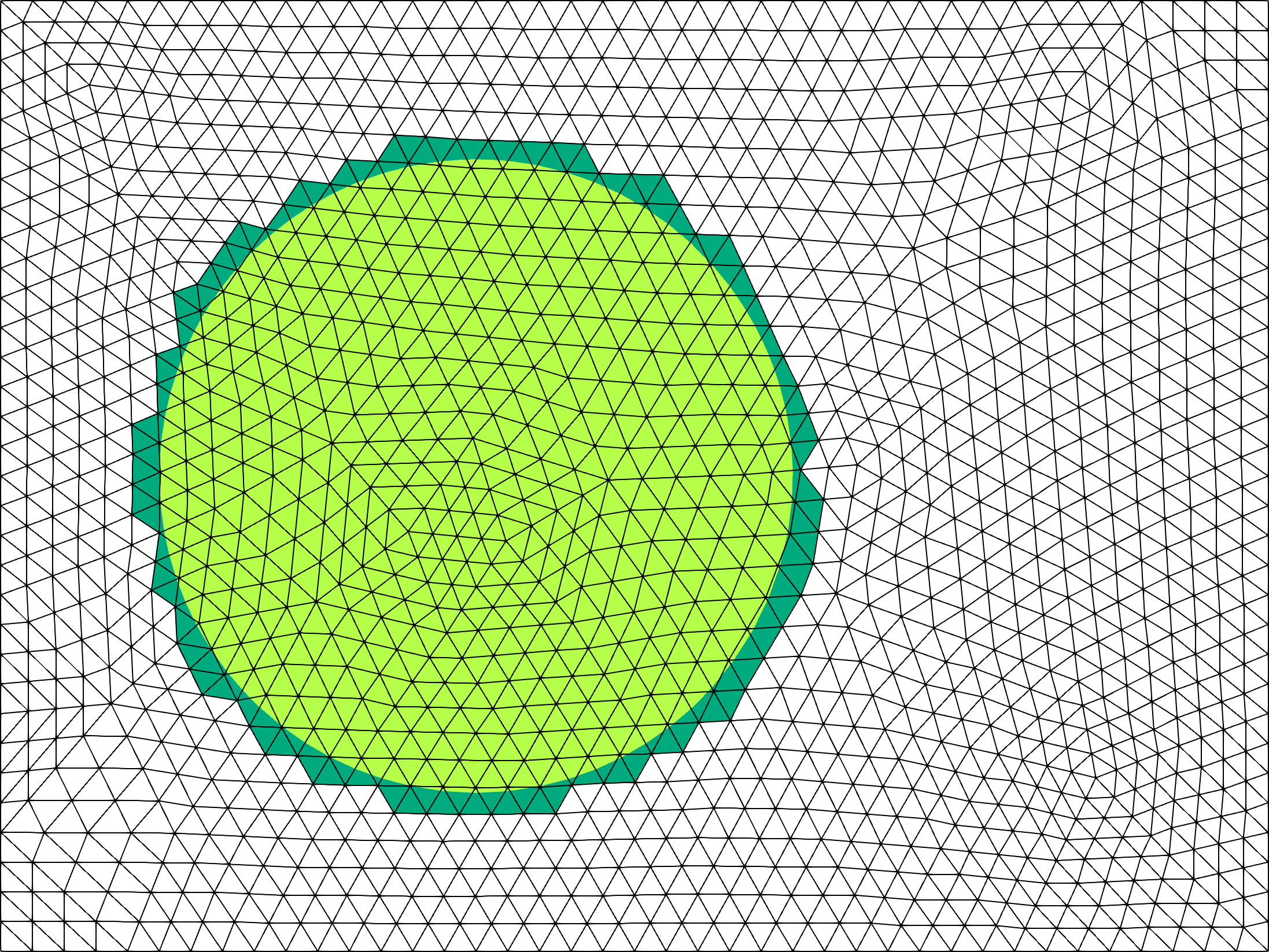
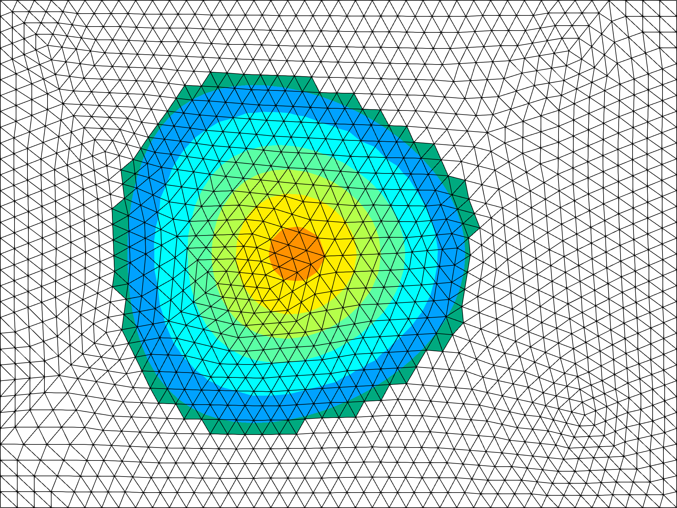
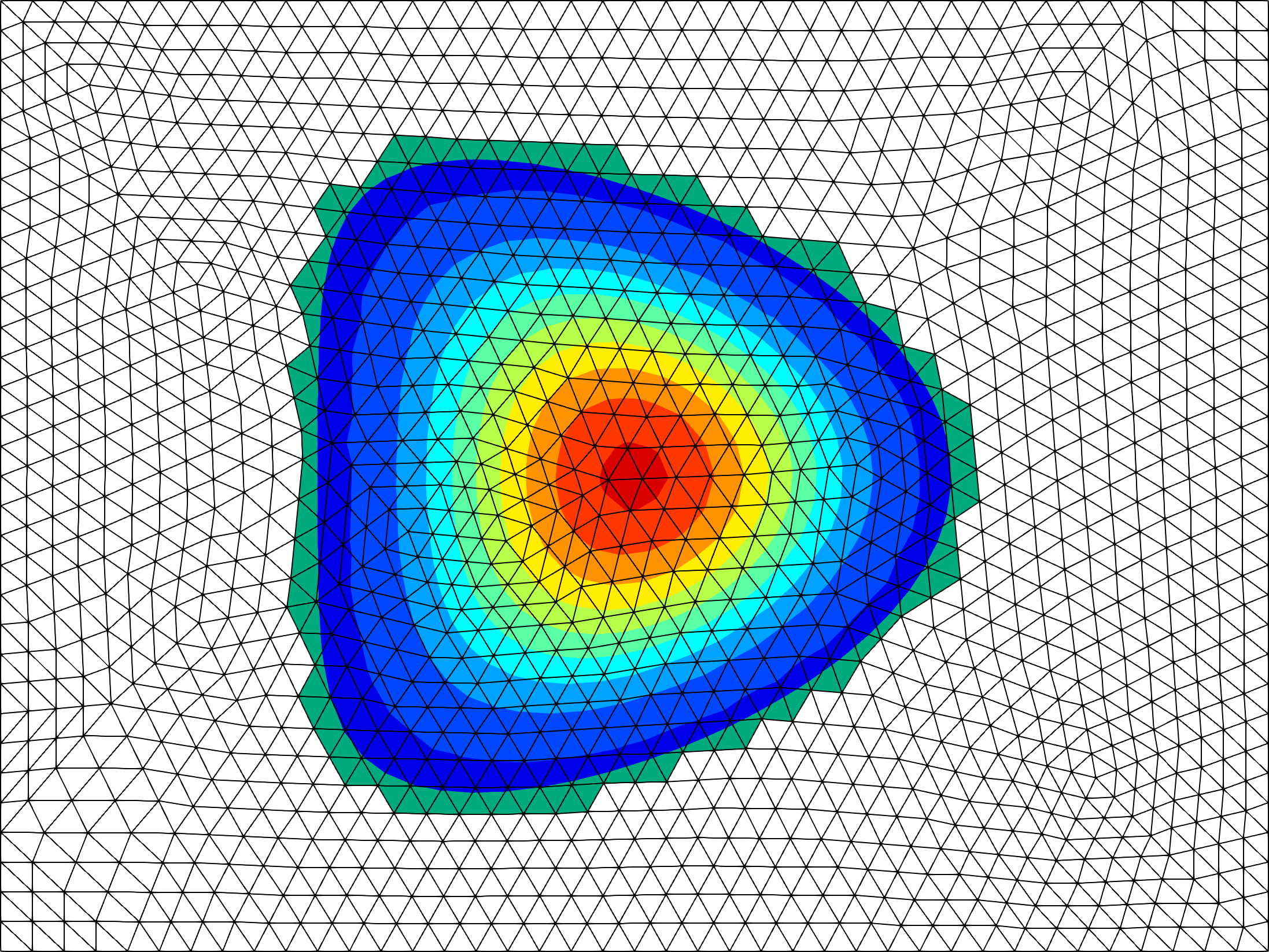
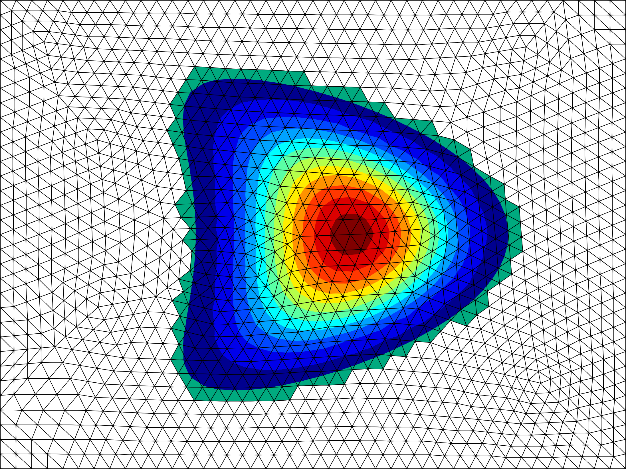
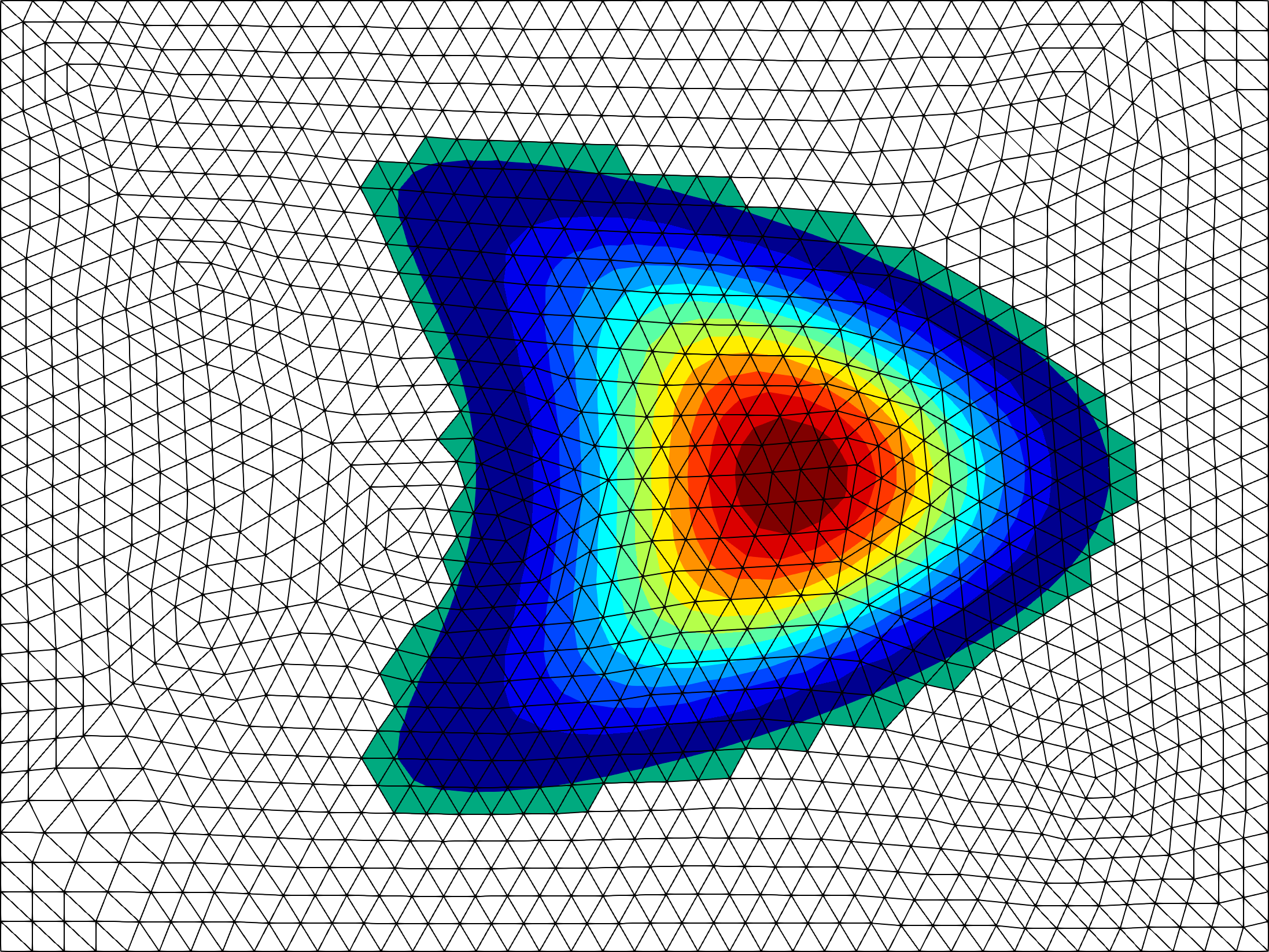
Figure 2. Discrete solution for the kite geometry at times $0.25T$ intervals with $h=0.4\cdot 2^{-2}$ and $\Delta t=0.5\cdot 2^{-6}$. Extension elements in $\pazocal{T}_{\pazocal{S}^{\pm}_{\delta}}^{n}$ are marked in green.

Set-up

We take the background domain as $\widetilde{\Omega}=(-1.5,2.5)\times(-1.5,1.5)$ and $T=1$. The level set function and transport field are given by

$$\rho(\bm{x},t)=\big{(}(1-\bm{x}_{2})^{2}t,0\big{)}^{T},\quad\phi(\bm{x},t)=\|\bm{x}-\rho(\bm{x},t)\|_{2}-R,\quad\bm{w}(\bm{x},t)=\partial_{t}\rho(\bm{x},t),$$

with $R=1$. The right-hand side forcing term is taken such that the exact solution is

$$u_{ex}(\bm{x},t)=\cos(\pi\|\bm{x}-\rho(\bm{x},t)\|_{2}/R)\sin(t\pi/2).$$

The viscosity is chosen to be $\nu=0.2$. The initial mesh size and time step are $h=0.4$ and $\Delta t=0.5$, respectively.

Convergence Study

We again consider a series of uniform refinements in space and time. The results for the BDF1 scheme can be found in Table 5, Table 6 for the $L^{2}(L^{2})$- and $L^{2}(H^{2})$-norms, respectively. The results for the BDF2 scheme are presented in Table 7, and Table 8.

For the results of the BDF1 scheme in the $L^{2}(L^{2})$-norm, we again observe optimal linear convergence in time on the finest mesh and linear convergence for combined mesh and time step refinement, indicating that the temporal error is dominating in this case. In the $L^{2}(H^{1})$-norm, the convergence with respect to the time-step is less than optimal, with both $\text{eoc}_{t}=\text{eoc}_{xt}\approx 0.7$.

For the BDF2 scheme, we see that for the $L^{2}(L^{2})$-norm error, the order of convergence in time ($\text{eoc}_{t}$) starts sub-optimal but increases to $1.84$. This is also reflected in $\text{eoc}_{xt}$, which is only around $2$ after the first level of refinement. This suggests that the time step really needs to be taken sufficiently small. Regarding the error $L^{2}(H^{1})$-norm, we again have suboptimal convergence in time on the fines mesh with $\text{eoc}_{t}\approx 1$. However, we see that $\text{eoc}_{xxt}$ approaches the optimal value of 2 under refinement. This again suggests that the time-step is not sufficiently small on the coarser time levels and that optimal convergence in time can only be realised in combination with mesh refinement.

Table 5. Convergence results for the BDF1 scheme in the $L^{2}(L^{2})$ norm for the kite geometry test case in Section 4.2

$L_{t}$\$L_{x}$	0	1	2	3	4	5	$\text{eoc}_{t}$
0	$6.08\text{\times}{10}^{-01}$	$4.60\text{\times}{10}^{-01}$	$4.25\text{\times}{10}^{-01}$	$4.17\text{\times}{10}^{-01}$	$4.15\text{\times}{10}^{-01}$	$4.14\text{\times}{10}^{-01}$	–
1	$3.45\text{\times}{10}^{-01}$	$2.55\text{\times}{10}^{-01}$	$2.27\text{\times}{10}^{-01}$	$2.20\text{\times}{10}^{-01}$	$2.18\text{\times}{10}^{-01}$	$2.18\text{\times}{10}^{-01}$	0.93
2	$2.50\text{\times}{10}^{-01}$	$1.45\text{\times}{10}^{-01}$	$1.23\text{\times}{10}^{-01}$	$1.17\text{\times}{10}^{-01}$	$1.16\text{\times}{10}^{-01}$	$1.16\text{\times}{10}^{-01}$	0.90
3	$2.05\text{\times}{10}^{-01}$	$9.43\text{\times}{10}^{-02}$	$6.70\text{\times}{10}^{-02}$	$6.23\text{\times}{10}^{-02}$	$6.14\text{\times}{10}^{-02}$	$6.14\text{\times}{10}^{-02}$	0.92
4	$1.82\text{\times}{10}^{-01}$	$6.99\text{\times}{10}^{-02}$	$3.83\text{\times}{10}^{-02}$	$3.28\text{\times}{10}^{-02}$	$3.19\text{\times}{10}^{-02}$	$3.18\text{\times}{10}^{-02}$	0.95
5	$1.71\text{\times}{10}^{-01}$	$5.82\text{\times}{10}^{-02}$	$2.40\text{\times}{10}^{-02}$	$1.74\text{\times}{10}^{-02}$	$1.64\text{\times}{10}^{-02}$	$1.62\text{\times}{10}^{-02}$	0.97
6	$1.66\text{\times}{10}^{-01}$	$5.34\text{\times}{10}^{-02}$	$1.74\text{\times}{10}^{-02}$	$9.56\text{\times}{10}^{-03}$	$8.43\text{\times}{10}^{-03}$	$8.24\text{\times}{10}^{-03}$	0.98
$\text{eoc}_{x}$	–	1.63	1.62	0.87	0.18	0.03
$\text{eoc}_{xt}$	–	1.25	1.12	1.03	1.00	0.99

Table 6. Convergence results for the BDF1 scheme in the $L^{2}(H^{1})$ norm for the kite geometry test case in Section 4.2

$L_{t}$\$L_{x}$	0	1	2	3	4	5	$\text{eoc}_{t}$
0	$2.40\text{\times}{10}^{00}$	$1.93\text{\times}{10}^{00}$	$1.88\text{\times}{10}^{00}$	$1.91\text{\times}{10}^{00}$	$1.94\text{\times}{10}^{00}$	$1.98\text{\times}{10}^{00}$	–
1	$1.71\text{\times}{10}^{00}$	$1.40\text{\times}{10}^{00}$	$1.33\text{\times}{10}^{00}$	$1.34\text{\times}{10}^{00}$	$1.37\text{\times}{10}^{00}$	$1.42\text{\times}{10}^{00}$	0.48
2	$1.45\text{\times}{10}^{00}$	$1.04\text{\times}{10}^{00}$	$8.99\text{\times}{10}^{-01}$	$8.65\text{\times}{10}^{-01}$	$9.01\text{\times}{10}^{-01}$	$9.54\text{\times}{10}^{-01}$	0.57
3	$1.32\text{\times}{10}^{00}$	$8.58\text{\times}{10}^{-01}$	$6.21\text{\times}{10}^{-01}$	$5.46\text{\times}{10}^{-01}$	$5.65\text{\times}{10}^{-01}$	$6.20\text{\times}{10}^{-01}$	0.62
4	$1.26\text{\times}{10}^{00}$	$7.76\text{\times}{10}^{-01}$	$4.77\text{\times}{10}^{-01}$	$3.59\text{\times}{10}^{-01}$	$3.45\text{\times}{10}^{-01}$	$3.81\text{\times}{10}^{-01}$	0.70
5	$1.23\text{\times}{10}^{00}$	$7.41\text{\times}{10}^{-01}$	$4.16\text{\times}{10}^{-01}$	$2.53\text{\times}{10}^{-01}$	$2.18\text{\times}{10}^{-01}$	$2.27\text{\times}{10}^{-01}$	0.75
6	$1.22\text{\times}{10}^{00}$	$7.28\text{\times}{10}^{-01}$	$3.93\text{\times}{10}^{-01}$	$2.10\text{\times}{10}^{-01}$	$1.41\text{\times}{10}^{-01}$	$1.40\text{\times}{10}^{-01}$	0.70
$\text{eoc}_{x}$	–	0.74	0.89	0.90	0.58	0.00
$\text{eoc}_{xt}$	–	0.72	0.75	0.79	0.72	0.64

Table 7. Convergence results for the BDF2 scheme in the $L^{2}(L^{2})$ norm for the kite geometry test case in Section 4.2

$L_{t}$\$L_{x}$	0	1	2	3	4	5	$\text{eoc}_{t}$
0	$6.20\text{\times}{10}^{-01}$	$4.95\text{\times}{10}^{-01}$	$4.27\text{\times}{10}^{-01}$	$3.85\text{\times}{10}^{-01}$	$3.62\text{\times}{10}^{-01}$	$3.51\text{\times}{10}^{-01}$	–
1	$4.16\text{\times}{10}^{-01}$	$2.56\text{\times}{10}^{-01}$	$1.90\text{\times}{10}^{-01}$	$1.64\text{\times}{10}^{-01}$	$1.52\text{\times}{10}^{-01}$	$1.46\text{\times}{10}^{-01}$	1.27
2	$2.45\text{\times}{10}^{-01}$	$1.33\text{\times}{10}^{-01}$	$7.80\text{\times}{10}^{-02}$	$6.02\text{\times}{10}^{-02}$	$5.45\text{\times}{10}^{-02}$	$5.22\text{\times}{10}^{-02}$	1.48
3	$2.01\text{\times}{10}^{-01}$	$7.15\text{\times}{10}^{-02}$	$3.49\text{\times}{10}^{-02}$	$2.06\text{\times}{10}^{-02}$	$1.68\text{\times}{10}^{-02}$	$1.59\text{\times}{10}^{-02}$	1.71
4	$1.81\text{\times}{10}^{-01}$	$5.88\text{\times}{10}^{-02}$	$1.89\text{\times}{10}^{-02}$	$8.23\text{\times}{10}^{-03}$	$5.07\text{\times}{10}^{-03}$	$4.46\text{\times}{10}^{-03}$	1.84
5	$1.71\text{\times}{10}^{-01}$	$5.41\text{\times}{10}^{-02}$	$1.55\text{\times}{10}^{-02}$	$4.41\text{\times}{10}^{-03}$	$1.85\text{\times}{10}^{-03}$	$1.25\text{\times}{10}^{-03}$	1.84
6	$1.65\text{\times}{10}^{-01}$	$5.13\text{\times}{10}^{-02}$	$1.41\text{\times}{10}^{-02}$	$3.57\text{\times}{10}^{-03}$	$9.80\text{\times}{10}^{-04}$	$4.20\text{\times}{10}^{-04}$	1.57
$\text{eoc}_{x}$	–	1.69	1.87	1.98	1.86	1.22
$\text{eoc}_{xt}$	–	1.65	1.92	2.09	2.15	2.14

Table 8. Convergence results for the BDF2 scheme in the $L^{2}(H^{1})$ norm for the kite geometry test case in Section 4.2

$L_{t}$\$L_{x}$	0	1	2	3	4	5	$\text{eoc}_{t}$
0	$2.62\text{\times}{10}^{00}$	$2.20\text{\times}{10}^{00}$	$2.03\text{\times}{10}^{00}$	$1.96\text{\times}{10}^{00}$	$1.97\text{\times}{10}^{00}$	$2.02\text{\times}{10}^{00}$	–
1	$2.02\text{\times}{10}^{00}$	$1.45\text{\times}{10}^{00}$	$1.23\text{\times}{10}^{00}$	$1.17\text{\times}{10}^{00}$	$1.17\text{\times}{10}^{00}$	$1.22\text{\times}{10}^{00}$	0.73
2	$1.46\text{\times}{10}^{00}$	$1.02\text{\times}{10}^{00}$	$7.66\text{\times}{10}^{-01}$	$6.42\text{\times}{10}^{-01}$	$6.06\text{\times}{10}^{-01}$	$6.17\text{\times}{10}^{-01}$	0.98
3	$1.33\text{\times}{10}^{00}$	$8.04\text{\times}{10}^{-01}$	$5.46\text{\times}{10}^{-01}$	$3.69\text{\times}{10}^{-01}$	$2.98\text{\times}{10}^{-01}$	$2.92\text{\times}{10}^{-01}$	1.08
4	$1.27\text{\times}{10}^{00}$	$7.59\text{\times}{10}^{-01}$	$4.28\text{\times}{10}^{-01}$	$2.56\text{\times}{10}^{-01}$	$1.64\text{\times}{10}^{-01}$	$1.43\text{\times}{10}^{-01}$	1.03
5	$1.24\text{\times}{10}^{00}$	$7.38\text{\times}{10}^{-01}$	$4.03\text{\times}{10}^{-01}$	$2.06\text{\times}{10}^{-01}$	$1.16\text{\times}{10}^{-01}$	$7.68\text{\times}{10}^{-02}$	0.90
6	$1.22\text{\times}{10}^{00}$	$7.26\text{\times}{10}^{-01}$	$3.90\text{\times}{10}^{-01}$	$1.95\text{\times}{10}^{-01}$	$9.74\text{\times}{10}^{-02}$	$5.37\text{\times}{10}^{-02}$	0.52
$\text{eoc}_{x}$	–	0.75	0.90	1.00	1.00	0.86
$\text{eoc}_{xxt}$	–	–	1.42	1.65	1.89	1.94

4.3. Example 3: Colliding circles

This more advanced example consists of two circles that collide and separate again [26]. Consequently, this includes a topology change in the geometry and a discontinuous transport field. Here we do not have an analytical solution, However, we can track the conservation of our scalar quantity.

The geometry is described by the level set function

$$\phi(\bm{x},t)=\min\{\|\bm{x}-s_{1}(t)\|_{2},\|\bm{x}-s_{1}(t)\|_{2}\}-R,\text{ with }s_{1}(t)=(0,t-3/4)^{T},\;s_{1}(t)=(0,3/4-t)^{T}.$$

The radius is chosen as $R=0.5$ and $T=1.5$, such that $\phi(\bm{x},0)=\phi(\bm{x},T)$. The transport field is given by

$$\bm{w}=\begin{cases}(0,-1)^{T}&\text{if ($\bm{x}_{2}>0$ and $t\leq T/2$) or ($\bm{x}_{2}\leq 0$ and $t>T/2$)}\\ (0,1)^{T}&\text{if ($\bm{x}_{2}\leq 0$ and $t\leq T/2$) or ($\bm{x}_{2}>0$ and $t<T/2$)}.\end{cases}$$

The background domain considered is $\widetilde{\Omega}=(-0.6,0.6)\times(-1.35,1.35)$ and diffusion coefficient is chosen to be $0.1$. Finally, the initial condition is given as $u_{0}=\operatorname{sign}(\bm{x}_{2})$.

We take $h=0.07$, $\Delta t=T/80$ and use the BDF2 scheme. The results at intervals of $0.1T$ can be seen in Figure 3. Visually, these results match those presented in [26]; however, here we conserve the total of our scalar quantity up to machine precision in every time step. As in [26], mass is exchanged between the two domains, as soon as the ghost-penalty extension domains overlap, rather than when the domains overlap.

-1 1-
          

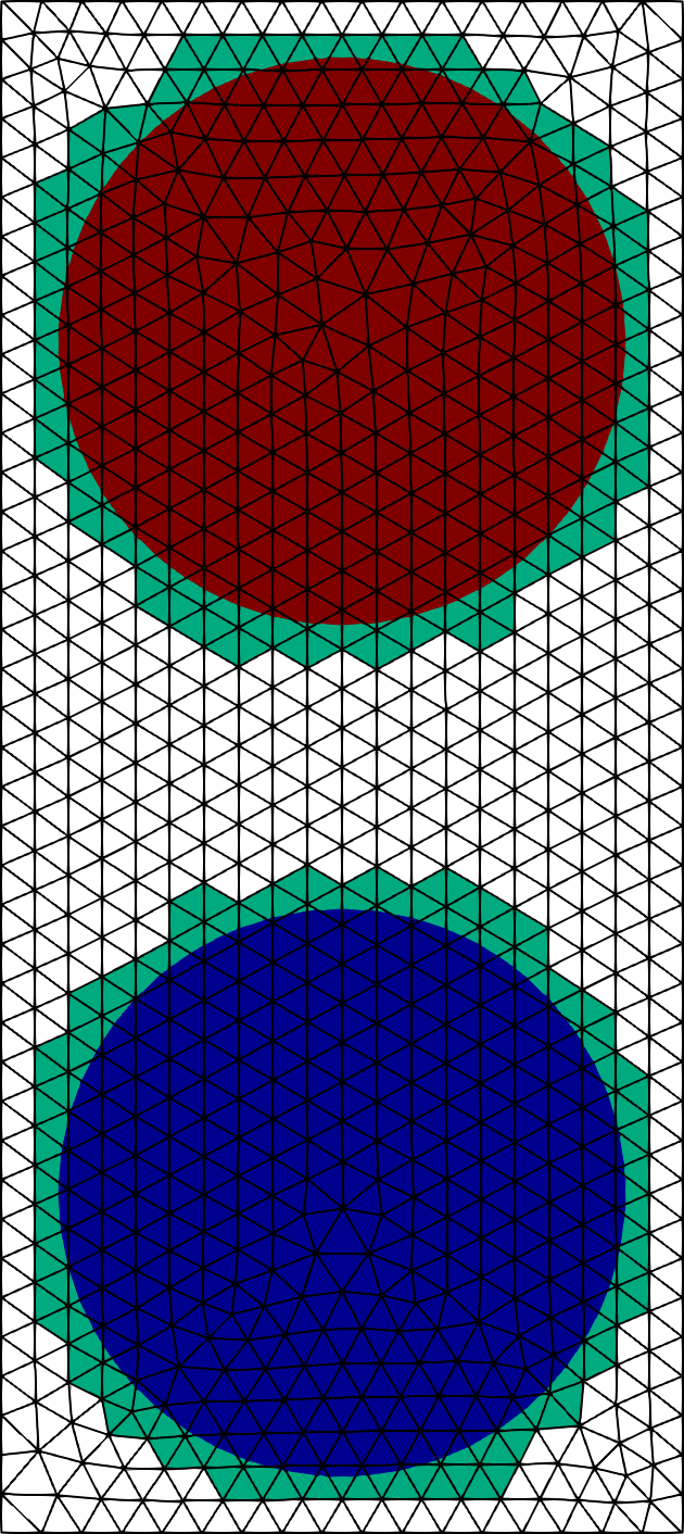
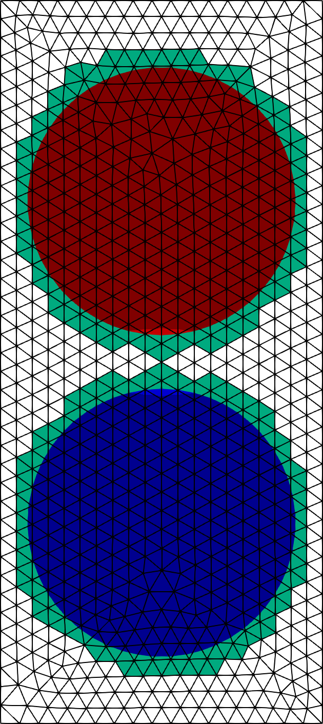
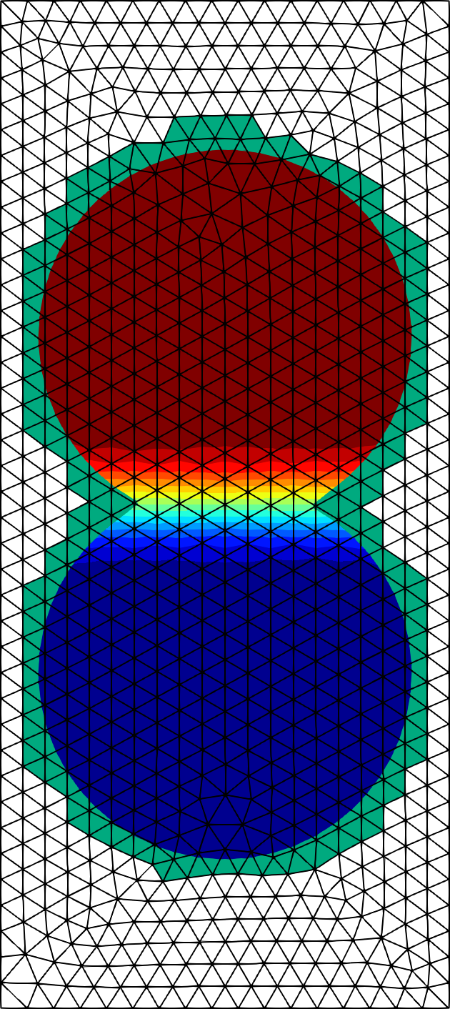
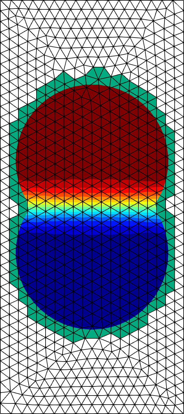
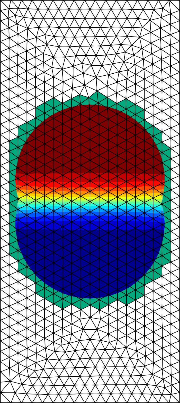
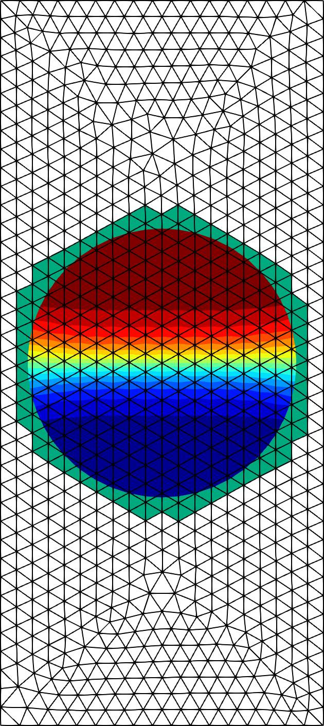
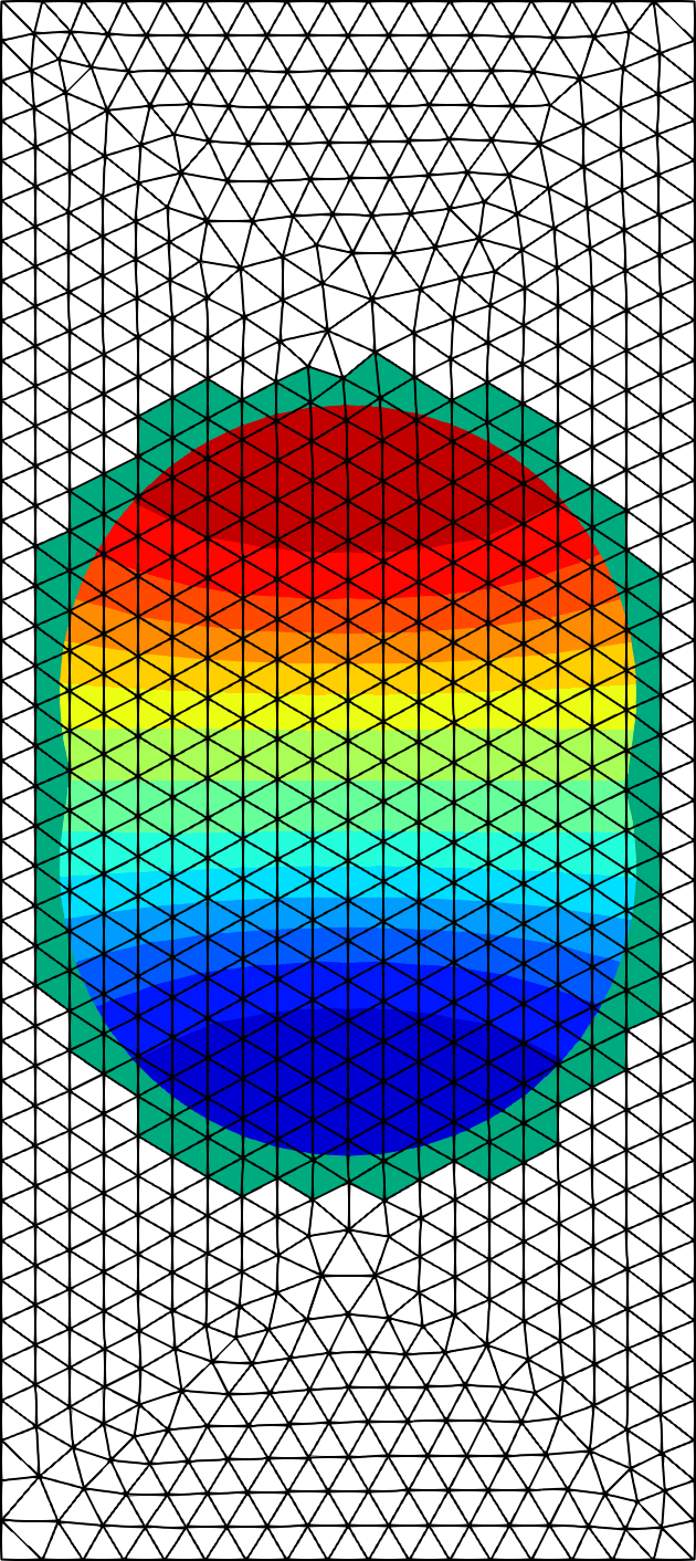
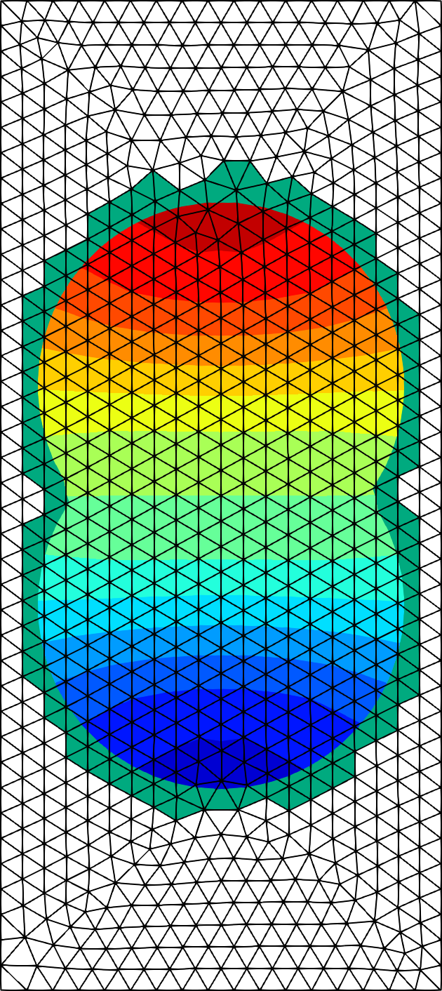
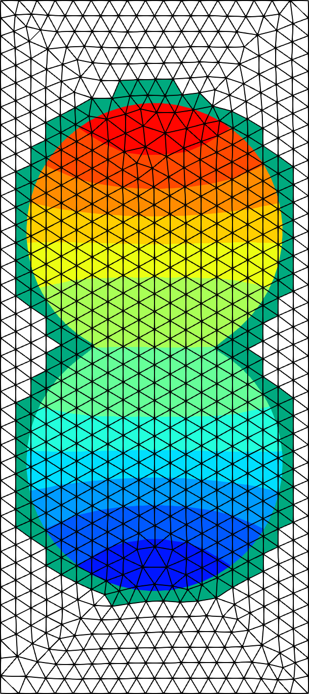
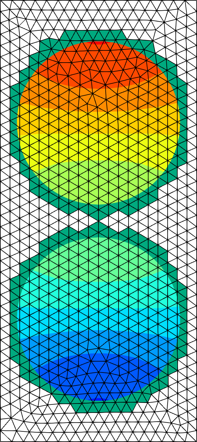
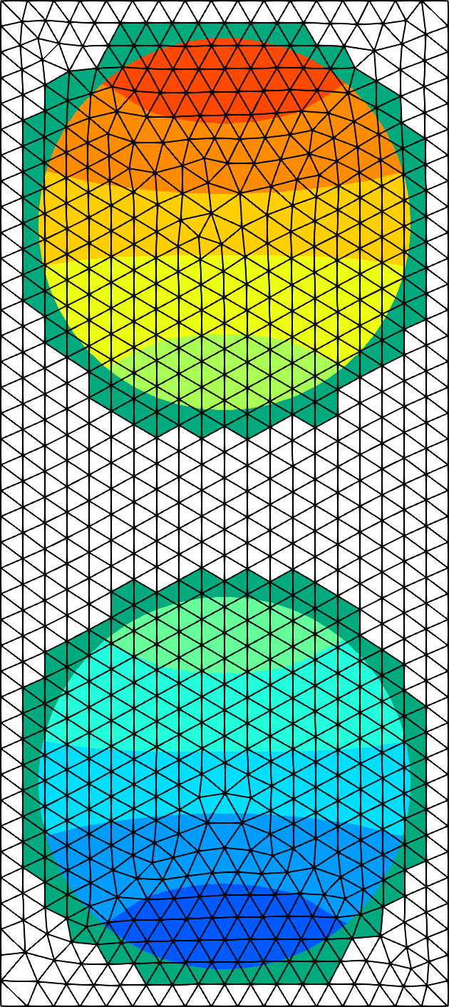
Figure 3. Discrete solution for the colliding circles test case in Section 4.3 at intervals of $0.1T$. Extension elements in $\pazocal{T}_{\pazocal{S}^{\pm}_{\delta}}^{n}$ are marked in green.

4.4. Example 4: Colliding spheres

Finally, we extend the previous example to three spatial dimensions. The geometry is now described by the level set function

$$\phi(\bm{x},t)=\min\{\|\bm{x}-s_{1}(t)\|_{2},\|\bm{x}-s_{1}(t)\|_{2}\}-R,\text{ with }s_{1}(t)=(0,0,t-3/4)^{T},\;s_{1}(t)=(0,0,3/4-t)^{T}.$$

The radius is chosen as $R=0.5$, the end time as $T=1.5$, and the transport field as

$$\bm{w}=\begin{cases}(0,0,-1)^{T}&\text{if ($\bm{x}_{3}>0$ and $t\leq T/2$) or ($\bm{x}_{3}\leq 0$ and $t>T/2$)}\\ (0,0,1)^{T}&\text{if ($\bm{x}_{3}\leq 0$ and $t\leq T/2$) or ($\bm{x}_{3}>0$ and $t<T/2$)}.\end{cases}$$

The background domain is $\widetilde{\Omega}=(-0.6,0.6)\times(-0.6,0.6)\times(-1.35,1.35)$, $\nu=0.1$ and $u_{0}=\operatorname{sign}(\bm{x}_{3})$.

We again take $h=0.07$, $\Delta t=T/80$ and use the BDF2 version of our time-stepping scheme. The results at intervals of $0.2T$ can be seen in Figure 4. We again observe the same behaviour as in the previous two-dimensional behaviour, and the total of the scalar quantity is preserved up to machine precision in every time step.

-1 1-
     

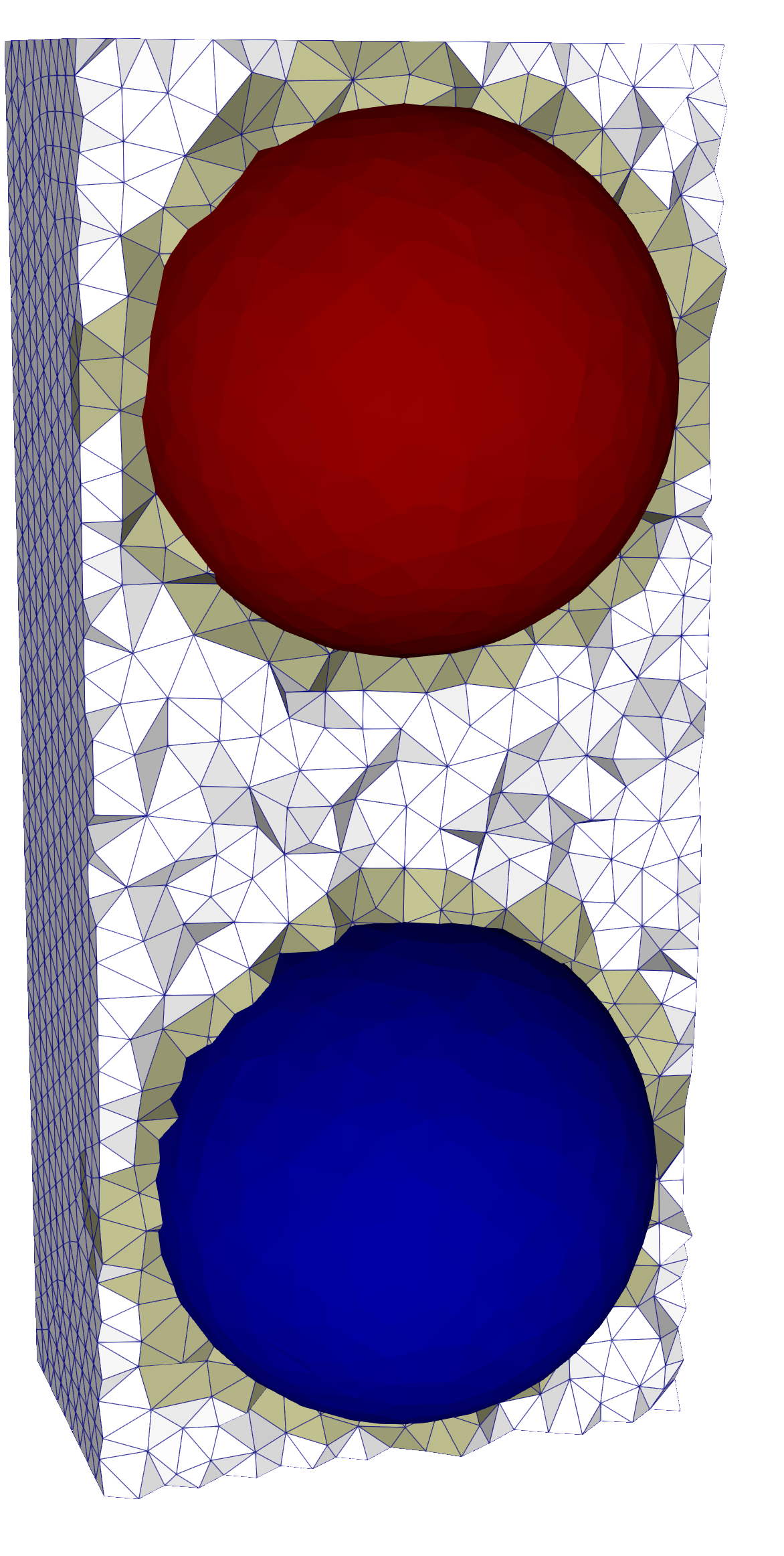
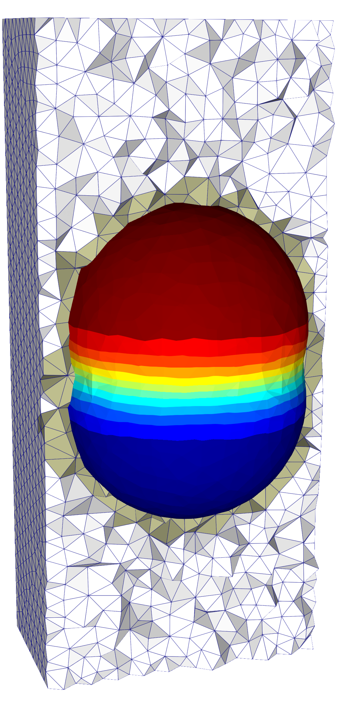
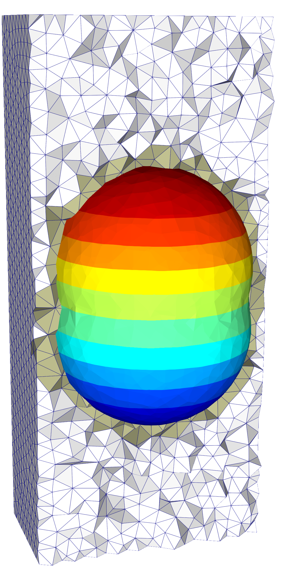
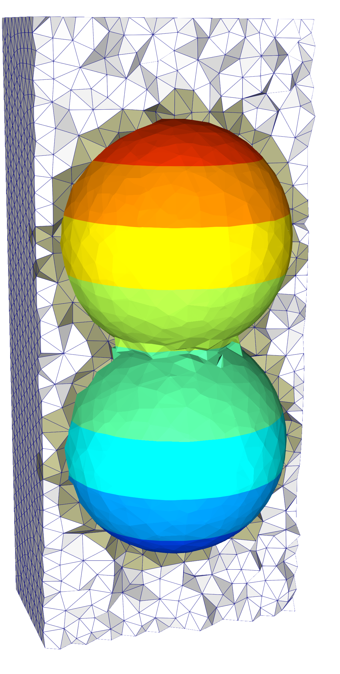
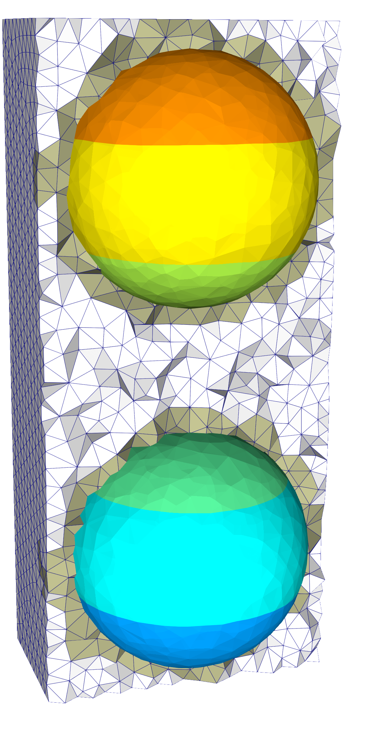
Figure 4. Discrete solution for the colliding sphere test case in Section 4.4 at intervals of $0.2T$. Extension elements in $\pazocal{T}_{\pazocal{S}^{\pm}_{\delta}}^{n}$ are marked in green.

Data Availability Statement

The code used to realise the numerical examples is freely available on github https://github.com/hvonwah/conserv-eulerian-moving-domian-repro and archived on zenodo https://doi.org/10.5281/zenodo.10951768.

References

• [1] Amal Alphonse, Charles M. Elliott and Björn Stinner “An abstract framework for parabolic PDEs on evolving spaces” In Portugal. Math. 72.1, 2015, pp. 1–46 DOI: 10.4171/PM/1955
• [2] M. Anselmann and M. Bause “Cut finite element methods and ghost stabilization techniques for space-time discretizations of the Navier–Stokes equations” In Internat. J. Numer. Methods Fluids Wiley, 2022 DOI: 10.1002/fld.5074
• [3] S. Badia, E. Neiva and F. Verdugo “Linking ghost penalty and aggregated unfitted methods” In Comput. Methods Appl. Mech. Engrg. 388 Elsevier BV, 2022, pp. 114232 DOI: 10.1016/j.cma.2021.114232
• [4] E. Burman “Ghost penalty” In C.R. Math. 348.21-22 Elsevier BV, 2010, pp. 1217–1220 DOI: 10.1016/j.crma.2010.10.006
• [5] E. Burman, S. Frei and A. Massing “Eulerian time-stepping schemes for the non-stationary Stokes equations on time-dependent domains” In Numer. Math. Springer ScienceBusiness Media LLC, 2022 DOI: 10.1007/s00211-021-01264-x
• [6] E. Burman and P. Hansbo “Fictitious domain finite element methods using cut elements: II. A stabilized Nitsche method” In Appl. Numer. Math. 62.4 Elsevier BV, 2012, pp. 328–341 DOI: 10.1016/j.apnum.2011.01.008
• [7] E. Burman et al. “CutFEM: Discretizing geometry and partial differential equations” In Internat. J. Numer. Methods Engrg. 104.7 Wiley, 2014, pp. 472–501 DOI: 10.1002/nme.4823
• [8] S. Claus and P. Kerfriden “A CutFEM method for two-phase flow problems” In Comput. Methods Appl. Mech. Engrg. 348 Elsevier BV, 2019, pp. 185–206 DOI: 10.1016/j.cma.2019.01.009
• [9] Ramon Codina, Guillaume Houzeaux, Herbert Coppola-Owen and Joan Baiges “The fixed-mesh ALE approach for the numerical approximation of flows in moving domains” In J. Comput. Phys. 228.5 Elsevier BV, 2009, pp. 1591–1611 DOI: 10.1016/j.jcp.2008.11.004
• [10] G. Dziuk and C.. Elliott $L^{2}$-estimates for the evolving surface finite element method” In Math. Comp. 82.281 American Mathematical Society (AMS), 2012, pp. 1–24 DOI: 10.1090/s0025-5718-2012-02601-9
• [11] T. Frachon, E. Nilsson and S. Zahedi “Divergence-free cut finite element methods for Stokes flow”, 2023 arXiv:2304.14230 [math.NA]
• [12] S. Frei and T. Richter “A second order time-stepping scheme for parabolic interface problems with moving interfaces” In ESAIM Math. Model. Numer. Anal. 51.4 EDP Sciences, 2017, pp. 1539–1560 DOI: 10.1051/m2an/2016072
• [13] S. Frei and M.. Singh “Analysis of an implicitly extended Crank-Nicolson scheme for the heat equation on a time-dependent domain”, 2022 arXiv:2203.06581 [math.NA]
• [14] T.-P. Fries and T. Belytschko “The extended/generalized finite element method: An overview of the method and its applications” In Internat. J. Numer. Methods Engrg. 84.3 Wiley, 2010, pp. 253–304 DOI: 10.1002/nme.2914
• [15] T.-P. Fries and S. Omerović “Higher-order accurate integration of implicit geometries” In Internat. J. Numer. Methods Engrg. 106.5 Wiley, 2015, pp. 323–371 DOI: 10.1002/nme.5121
• [16] Harald Garcke, Kei Fong Lam, Robert Nürnberg and Emanuel Sitka “A multiphase Cahn–Hilliard–Darcy model for tumour growth with necrosis” In Math. Models Methods Appl. Sci. 28.03 World Scientific Pub Co Pte Ltd, 2018, pp. 525–577 DOI: 10.1142/s0218202518500148
• [17] P. Hansbo, M.. Larson and S. Zahedi “A cut finite element method for coupled bulk-surface problems on time-dependent domains” In Comput. Methods Appl. Mech. Engrg. 307 Elsevier BV, 2016, pp. 96–116 DOI: 10.1016/j.cma.2016.04.012
• [18] Frédéric Hecht and Olivier Pironneau “An energy stable monolithic Eulerian fluid-structure finite element method” In Internat. J. Numer. Methods Fluids 85.7 Wiley, 2017, pp. 430–446 DOI: 10.1002/fld.4388
• [19] F. Heimann, C. Lehrenfeld and J. Preuß “Geometrically Higher Order Unfitted Space-Time Methods for PDEs on Moving Domains” In SIAM J. Sci. Comput. 45.2 Society for Industrial & Applied Mathematics (SIAM), 2023, pp. B139–B165 DOI: 10.1137/22m1476034
• [20] F. Heimann, C. Lehrenfeld, P. Stocker and H. Wahl “Unfitted Trefftz discontinuous Galerkin methods for elliptic boundary value problems” In ESAIM Math. Model. Numer. Anal. 57.5 EDP Sciences, 2023, pp. 2803–2833 DOI: 10.1051/m2an/2023064
• [21] J.. Heywood and R. Rannacher “Finite-element approximation of the nonstationary Navier-Stokes problem. Part IV: Error analysis for second-order time discretization” In SIAM J. Numer. Anal. 27.2 Society for Industrial & Applied Mathematics (SIAM), 1990, pp. 353–384 DOI: 10.1137/0727022
• [22] Cyrill W. Hirt, Anthony A. Amsden and J.. Cook “An arbitrary Lagrangian-Eulerian computing method for all flow speeds” In J. Comput. Phys. 14.3 Elsevier, 1974, pp. 227–253 DOI: 10.1016/0021-9991(74)90051-5
• [23] Gozel Judakova and Markus Bause “Numerical Investigation of Multiphase Flow inPipelines” In Internat. Journal. Mech. Mechatron. Engrg. 11.9, 2017 DOI: 10.5281/zenodo.1132012
• [24] C. Lehrenfeld “High order unfitted finite element methods on level set domains using isoparametric mappings” In Comput. Methods Appl. Mech. Engrg. 300 Elsevier BV, 2016, pp. 716–733 DOI: 10.1016/j.cma.2015.12.005
• [25] C. Lehrenfeld, F. Heimann, J. Preuß and H. Wahl “ngsxfem: Add-on to NGSolve for geometrically unfitted finite element discretizations” In J. Open Source Softw. 6.64 The Open Journal, 2021, pp. 3237 DOI: 10.21105/joss.03237
• [26] C. Lehrenfeld and M.. Olshanskii “An Eulerian finite element method for PDEs in time-dependent domains” In ESAIM Math. Model. Numer. Anal. 53.2 EDP Sciences, 2019, pp. 585–614 DOI: 10.1051/m2an/2018068
• [27] C. Lehrenfeld and A. Reusken “Analysis of a Nitsche XFEM-DG Discretization for a Class of Two-Phase Mass Transport Problems” In SIAM J. Numer. Anal. 51.2 Society for Industrial & Applied Mathematics (SIAM), 2013, pp. 958–983 DOI: 10.1137/120875260
• [28] Y. Lou and C. Lehrenfeld “Isoparametric Unfitted BDF–Finite Element Method for PDEs on Evolving Domains” In SIAM J. Numer. Anal. 60.4 Society for Industrial & Applied Mathematics (SIAM), 2021, pp. 2069–2098 DOI: 10.1137/21m142126x
• [29] A. Massing, M.. Larson, A. Logg and M.. Rognes “A stabilized Nitsche fictitious domain method for the Stokes problem” In J. Sci. Comput. 61.3 Springer Nature, 2014, pp. 604–628 DOI: 10.1007/s10915-014-9838-9
• [30] Arif Masud and Thomas J.. Hughes “A space-time Galerkin/least-squares finite element formulation of the Navier-Stokes equations for moving domain problems” In Comput. Methods Appl. Mech. Engrg. 146.1-2 Elsevier, 1997, pp. 91–126 DOI: 10.1016/S0045-7825(96)01222-4
• [31] B. Müller, F. Kummer and M. Oberlack “Highly accurate surface and volume integration on implicit domains by means of moment-fitting” In Internat. J. Numer. Methods Engrg. 96.8 Wiley, 2013, pp. 512–528 DOI: 10.1002/nme.4569
• [32] M. Neilan and M. Olshanskii “An Eulerian finite element method for the linearized Navier–Stokes problem in an evolving domain” In IMA J. Numer. Anal. Oxford University Press (OUP), 2024 DOI: 10.1093/imanum/drad105
• [33] M.. Olshanskii, A. Reusken and J. Grande “A Finite Element Method for Elliptic Equations on Surfaces” In SIAM J. Numer. Anal. 47.5 Society for Industrial & Applied Mathematics (SIAM), 2009, pp. 3339–3358 DOI: 10.1137/080717602
• [34] M.. Olshanskii, A. Reusken and X. Xu “An Eulerian Space-Time Finite Element Method for Diffusion Problems on Evolving Surfaces” In SIAM J. Numer. Anal. 52.3 Society for Industrial & Applied Mathematics (SIAM), 2014, pp. 1354–1377 DOI: 10.1137/130918149
• [35] M.. Olshanskii and D. Safin “Numerical integration over implicitly defined domains for higher order unfitted finite element methods” In Lobachevskii J. Math. 37.5 Pleiades Publishing Ltd, 2016, pp. 582–596 DOI: 10.1134/s1995080216050103
• [36] Jamshid Parvizian, Alexander Düster and Ernst Rank “Finite cell method: h-and p-extension for embedded domain problems in solid mechanics” In Comput. Mech. 41.1 Springer, 2007, pp. 121–133 DOI: 10.1007/s00466-007-0173-y
• [37] Fernando Porté-Agel, Majid Bastankhah and Sina Shamsoddin “Wind-Turbine and Wind-Farm Flows: A Review” In Bound.-Layer Meteorol. 174.1 Springer ScienceBusiness Media LLC, 2019, pp. 1–59 DOI: 10.1007/s10546-019-00473-0
• [38] J. Preuß “Higher order unfitted isoparametric space-time FEM on moving domains”, 2018 DOI: 10.25625/UACWXS
• [39] R.. Saye “High-Order Quadrature Methods for Implicitly Defined Surfaces and Volumes in Hyperrectangles” In SIAM J. Sci. Comput. 37.2 Society for Industrial & Applied Mathematics (SIAM), 2015, pp. A993–A1019 DOI: 10.1137/140966290
• [40] J. Schöberl “NETGEN an advancing front 2D/3D-mesh generator based on abstract rules” In Comput. Vis. Sci. 1.1 Springer Nature, 1997, pp. 41–52 DOI: 10.1007/s007910050004
• [41] J. Schöberl “C++11 implementation of finite elements in NGSolve”, 2014 URL: http://www.asc.tuwien.ac.at/~schoeberl/wiki/publications/ngs-cpp11.pdf
• [42] B. Schott “Stabilized cut finite element methods for complex interface coupled flow problems”, 2017 URL: http://mediatum.ub.tum.de?id=1304754
• [43] E.. Stein “Singular Integrals and Differentiability Properties of Functions” 30, Princeton Mathematical Series Princeton, NJ: Princeton University Press, 1970 URL: https://www.jstor.org/stable/j.ctt1bpmb07
• [44] Sankaran Sundaresan “Instabilities in Fluidized Beds” In Annu. Rev. Fluid Mech. 35.1 Annual Reviews, 2003, pp. 63–88 DOI: 10.1146/annurev.fluid.35.101101.161151
• [45] Tayfun E. Tezduyar, Mittal Behr, S. Mittal and J11530600745 Liou “A new strategy for finite element computations involving moving boundaries and interfaces—the deforming-spatial-domain/space-time procedure: II. Computation of free-surface flows, two-liquid flows, and flows with drifting cylinders” In Comput. Methods Appl. Mech. Engrg. 94.3 Elsevier, 1992, pp. 353–371 DOI: 10.1016/0045-7825(92)90060-W
• [46] Yuri Vassilevski et al. “Personalized Computational Hemodynamics: Models, Methods, and Applications for Vascular Surgery and Antitumor Therapy” Academic Press, 2020 DOI: 10.1016/c2017-0-02421-7
• [47] H. Wahl and T. Richter “An Eulerian time-stepping scheme for a coupled parabolic moving domain problem using equal order unfitted finite elements” In Proc. Appl. Math. Mech., 2023 DOI: 10.1002/pamm.202200003
• [48] H. Wahl and T. Richter “Error Analysis for a Parabolic PDE Model Problem on a Coupled Moving Domain in a Fully Eulerian Framework” In SIAM J. Numer. Anal. 61.1 Society for Industrial & Applied Mathematics (SIAM), 2023, pp. 286–314 DOI: 10.1137/21m1458417
• [49] H. Wahl, T. Richter and C. Lehrenfeld “An unfitted Eulerian finite element method for the time-dependent Stokes problem on moving domains” In IMA J. Numer. Anal. 42.3 Oxford University Press (OUP), 2021, pp. 2505–2544 DOI: 10.1093/imanum/drab044