Homogeneous spacetime with shear viscosity

Abstract

We study the homogeneous and anisotropic evolution of spacetime driven by perfect fluid with shear viscosity. We obtain exact solutions by considering the simplest form of the equation of state wherein the pressure and the shear stress are proportional to the energy density individually. The solutions represent Bianchi type-I cosmology of which the special case becomes Bianchi type-VII. We find that the initial singularity can be removed only for the Bianchi type-VII.

I Introduction

In relativistic cosmology, people introduce perfect fluid to model a homogeneous and isotropic universe (MTW, ). It is, however, plausible to consider that the Universe in the beginning might have had anisotropy which had died out in the course of evolution resulting in the present Universe. More realistic models, therefore, include dissipative processes which are caused by bulk and shear viscosities. Misner has argued that the neutrino viscosity may reduce the shear anisotropy present in the early universe (Misner:1967uu, ). Later, However, Stewart (Stewart1968, ; Stewart1969, ) and Doroshkevich et. al. (Doro1968, ) pointed out that Misner’s findings were based on the assumption that the anisotropy in the early universe is small. Stewart argued that, for large anisotropy, the viscous effects of neutrinos are inefficient in reducing the shear completely (Stewart1968, ).

Shear viscosity usually manifests as anisotropy. In this work, we shall consider both diagonal and off-diagonal components of the energy-momentum tensor modelled by shear viscosity. It is quite natural to consider the shear viscosity in the realistic astrophysical situations involving fluid plasma. It is also natural to consider it in cosmology; however, as the current universe exhibits very small anisotropy, people often ignore it simply for convenience. In cosmological perturbation theories, an anisotropic tensor field which represents the shear viscosity inevitably arises in theories higher than linear order (Noh:2004bc, ; Hwang:2007ni, ; Hwang:2017oxa, ).

In Eckart’s theory the energy-momentum tensor of fluid is given by (Eckart:1940te, ; MTW, ; Pimentel, )

$$T^{\mu\nu}=\rho u^{\mu}u^{\nu}+(p-\xi\Theta)h^{\mu\nu}+q^{\mu}u^{\nu}+q^{\nu}u^{\mu}-2\eta\sigma^{\mu\nu}.$$ (1)

Here, $\xi$ and $\eta$ are the bulk and the shear viscosity coefficients, $q^{\mu}$ is the heat-flux four-vector, $u^{\mu}$ is the four-velocity of fluid, $h_{\mu\nu}=g_{\mu\nu}+u_{\mu}u_{\nu}$ is the projection tensor, $\Theta=u^{\mu}_{;\mu}$ is the expansion, and $\sigma_{\mu\nu}=(u_{\mu;\delta}h^{\delta}_{\nu}+u_{\nu;\delta}h^{\delta}_{\mu})/2-\Theta h_{\mu\nu}/3$ is the symmetric traceless shear tensor. The above energy-momentum consists of three components; the perfect fluid component, $T^{\mu\nu}_{\rm pf}=\rho u^{\mu}u^{\nu}+ph^{\mu\nu}$ makes , the heat-flux component, $T^{\mu\nu}_{\rm heat}=q^{\mu}u^{\nu}+q^{\nu}u^{\mu}$, and the viscosity component, $T^{\mu\nu}_{\rm visc}=-\xi\Theta h^{\mu\nu}-2\eta\sigma^{\mu\nu}$. It is to be noted that the shear tensor contributes to both the spatial diagonal and off-diagonal components of the energy-momentum tensor in general while the bulk viscosity contributes to the diagonal components only.

Anisotropic cosmological models with both bulk and shear viscosity has been studied in the literature in Refs. (VC1, ; VC1-1, ; VC3, ; VC2, ; VC4, ; VC5, ; VC6, ), although exact solutions are not much known. Most of the available exact solutions are those with non-zero bulk viscosity; exact solutions with non-zero shear viscosity are very few. Besides the equation of state between the pressure and the energy density, most of these works assume a ‘second equation of state’ associated with the viscosity coefficient $\eta$. Belinski and Khalatnikov (VC1-1, ) studied Bianchi type-I cosmology with both bulk and shear viscosities. In the asymptotic limits of both small and large $\rho$, they considered $\eta\propto\rho^{A}$. They showed that the viscosities were not capable of removing the cosmological singularity. They found that the curvature invariants diverge at the singularity while the energy density vanishes. Similar results were obtained for some cases in Ref. VC3 in which the authors studied Bianchi type-I cosmology with stiff matter ($p=\rho$) with $\eta\propto\rho^{A}$. Anisotropic cosmology with $\eta\propto\rho$ was studied in Ref. VC2 , although a complete exact solution was not obtained. Banerjee et. al. (VC5, ) considered the shear to be proportional to the expansion, i.e., $\sigma^{\mu\nu}\sigma_{\mu\nu}\propto\Theta^{2}$, and studied exact cosmological solutions of several Bianchi types. Anisotropic cosmological models with $\eta\propto\rho^{A}$ and $\eta\propto H$, where $H$ is the average Hubble parameter, were studied in Ref. (VC6, ). It is to be noted that $\eta$ does not have any specific form of equation of state. Most of the works in the literature utilize certain simplifying assumptions for the equation of state to get the exact solutions. In this work, we shall impose the equation of state for viscosity directly to the off-diagonal stress term $\eta\sigma^{\mu\nu}$. In particular, we consider that this off-diagonal term is proportional to the energy density.

In Ref. Cho:2022rgs , we studied anisotropic cosmology and obtained exact solutions by considering an energy-momentum tensor with all the spatial off-diagonal terms to be the same. We considered two equations of states $p=\alpha\rho$ and $\sigma=T^{i}_{j\;\rm shear\;visc}(i\neq j)=\beta\rho$. We found that the spacetime expands less rapidly at late times than the usual Friedmann universe as the energy density drops faster due to the transfer to the shear stress. We found also that the initial big-bang singularity can be removed in the parameter region $1+\alpha+2\beta\leq 0$. In the present work, we study anisotropic cosmology with an energy-momentum tensor containing only one non-zero off-diagonal stress. If we perform the diagonalization of the set-up, the present case corresponds to the Bianchi type-I which has anisotropy along all three spatial directions (the previous work is Bianchi type-VII which is a special case of Bianchi type-I). We obtain exact solution by considering the same equations of state as in the previous work. We find that the initial singularity always exists in the present case.

The paper is organized as follows. In Sec. II, we introduce our model and obtain the exact solutions of the Einstein’s field equation. In Sec. III, we analyze the early-time behaviour of the solutions, the energy density and the Kretschmann scalar, and discuss the effect of the shear stress on the singularity structure of the solution. We also discuss the connection of the singularity structure with various energy conditions. In Sec. IV, we analyze the late-time behaviour of the solutions and compare with that of the Friedmann universe and conclude in Sec. V.

II Model and field equations

In Ref. Cho:2022rgs , we studied anisotropic cosmology and obtained exact solutions by considering an energy-momentum tensor with all the spatial off-diagonal terms to be the same. In this work, we consider a fluid whose energy-momentum tensor has only one spatial off-diagonal component and is given by

$$T^{\mu}_{\nu}=\begin{bmatrix}\;-\rho\;\;\;\;&0\;\;\;\;\;&0\;\;\;\;\;&0\;\;\;\;\\ 0&p_{1}+\sigma_{1}&\sigma&0\\ 0&\sigma&p_{1}+\sigma_{1}&0\\ 0&0&0&p_{2}-2\sigma_{1}\end{bmatrix},$$ (2)

where the energy density $\rho$, the pressures $p_{1}$ and $p_{2}$, and the stresses $\sigma$ and $\sigma_{1}$ depend only on time $t$. Later, we set $p_{1}=p_{2}$. The above energy-momentum tensor can solves the Einstein equations consistently if we consider a metric of following ansatz:

$$ds^{2} =-dt^{2}+a^{2}(t)\left(dx^{2}+dy^{2}\right)+2b(t)dxdy+e^{2}(t)dz^{2}$$ (3)

$$=-dt^{2}+\frac{1}{2}\left[c^{2}(t)+d^{2}(t)\right]\left(dx^{2}+dy^{2}\right)+\left[d^{2}(t)-c^{2}(t)\right]dxdy+e^{2}(t)dz^{2},$$ (4)

where we rewrote the metric in the last step by defining $a^{2}=(c^{2}+d^{2})/2$ and $b=(d^{2}-c^{2})/2$ as it is easier to solve the field equations using the metric in Eq. (4). The three-volume density is given by ${\cal V}_{3}=(a^{4}-b^{2})^{1/2}e=cde$. For the co-moving fluid four-velocity $u^{\mu}=(u^{t},u^{x},u^{y},u^{z})=(1,0,0,0)$, the expansion and the nonzero components of the shear tensor become $\Theta=\left(\dot{c}/c+\dot{d}/d+\dot{e}/e\right)$, $\sigma^{x}_{y}=\sigma^{y}_{x}=-(\dot{c}/c-\dot{d}/d)/2$ and $\sigma^{x}_{x}=\sigma^{y}_{y}=-\sigma^{z}_{z}/2=(\dot{c}/c+\dot{d}/d-2\dot{e}/e)/6$. It is to be noted that, the energy-momentum tensor (2) takes the form (1) if we set $\eta\neq 0$, $\xi=0$, $q^{\mu}=0$, $\sigma=\eta(\dot{c}/c-\dot{d}/d)$, $\sigma_{1}=-\eta(\dot{c}/c+\dot{d}/d-2\dot{e}/e)/3$ and $p_{1}=p_{2}=p$.

We now consider the isotropic pressure $p_{1}=p_{2}=p$. The Einstein field equations require $e^{2}=c^{1+3n}d^{1-3n}$, where $n$ is a constant. This gives $\sigma_{1}=n\sigma$.

One can transform both the metric and the energy-momentum tensor to diagonal form by suitable coordinate transformations. The coordinate transformations,

$$X=\frac{1}{\sqrt{2}}(x+y),\quad Y=\frac{1}{\sqrt{2}}(x-y),\quad Z=z,$$ (5)

transforms the metric (4) to the Bianchi type I metric,

$$ds^{2}=-dt^{2}+d^{2}(t)dX^{2}+c^{2}(t)dY^{2}+c^{1+3n}(t)d^{1-3n}(t)dZ^{2}.$$ (6)

Similarly, the energy-momentum tensor (2) is transformed to

$$T^{\mu}_{\nu}=\begin{bmatrix}\;-\rho\;\;\;\;&0\;\;\;\;\;&0\;\;\;\;\;&0\;\;\;\;\\ 0&p+(n+1)\sigma&0&0\\ 0&0&p+(n-1)\sigma&0\\ 0&0&0&p-2n\sigma\end{bmatrix}.$$ (7)

The Einstein’s equations in the diagonal form are equivalent to the ones in the off-diagonal form. It is to be noted that, for $n=\pm 1/3$, both the diagonal metric and the diagonal energy-momentum tensor reduce to the ones discussed in our earlier work in Ref. Cho:2022rgs . Thus, for $n=\pm 1/3$, the solution obtained in the present work also reduces to the one obtained in Ref. Cho:2022rgs .

The components of the Einstein’s equation $G^{\mu}_{\nu}=T^{\mu}_{\nu}$ ($8\pi G=1$) yield

$$(1+3n)\frac{\dot{c}^{2}}{c^{2}}+4\frac{\dot{c}}{c}\frac{\dot{d}}{d}+(1-3n)\frac{\dot{d}^{2}}{d^{2}} =2\rho,$$ (8)

$$2(1+n)\frac{\ddot{c}}{c}+2(1-n)\frac{\ddot{d}}{d}+n(1+3n)\frac{\dot{c}^{2}}{c^{2}}+2(1-3n^{2})\frac{\dot{c}}{c}\frac{\dot{d}}{d}-n(1-3n)\frac{\dot{d}^{2}}{d^{2}} =-2p,$$ (9)

$$2\frac{\ddot{c}}{c}-2\frac{\ddot{d}}{d}+(1+3n)\frac{\dot{c}^{2}}{c^{2}}-6n\frac{\dot{c}}{c}\frac{\dot{d}}{d}-(1-3n)\frac{\dot{d}^{2}}{d^{2}} =-4\sigma.$$ (10)

We, therefore, have three equations for the five unknowns $c$, $d$, $\rho$, $p$ and $\sigma$. We need two more equations to consistently solve the field equations. For that, we consider following two equations of state in the same way as in Ref. Cho:2022rgs ,

$$p=\alpha\rho,\qquad\sigma=\beta\rho.$$ (11)

With this, we manipulate the field equations and integrate them (see Appendix A). After integrating once, the field equations with new variables $u=c^{\bar{n}_{1}}d^{\bar{n}_{2}}$ and $v=c^{n_{1}}d^{n_{2}}$ reduce to [see Eqs. (56), (57) and (58)]

$$\frac{\dot{u}}{u}=\frac{A_{1}}{u^{\sqrt{3}/4}v^{\sqrt{3}/4-s_{2}}},$$ (12)

$$\frac{\dot{v}}{v}=\frac{A_{2}}{u^{\sqrt{3}/4-s_{1}}v^{\sqrt{3}/4}},$$ (13)

$$\rho=\frac{A_{1}A_{2}/4}{u^{\sqrt{3}/2-s_{1}}v^{\sqrt{3}/2-s_{2}}},$$ (14)

where $A_{1}$ and $A_{2}$ are integration constants and

$$s_{1}=\frac{1}{4}\left[\sqrt{3}(1-\alpha)-2\sqrt{1+3n^{2}}\beta\right],\quad s_{2}=\frac{1}{4}\left[\sqrt{3}(1-\alpha)+2\sqrt{1+3n^{2}}\beta\right],$$ (15)

$$n_{1}=\sqrt{3}(1+n)+\sqrt{1+3n^{2}},\quad n_{2}=\sqrt{3}(1-n)-\sqrt{1+3n^{2}},$$ (16)

$$\bar{n}_{1}=\sqrt{3}(1+n)-\sqrt{1+3n^{2}},\quad\bar{n}_{2}=\sqrt{3}(1-n)+\sqrt{1+3n^{2}}.$$ (17)

From Eqs. (12) and (13), we obtain for later use,

$$u^{s_{1}-1}\dot{u}=\frac{A_{1}}{A_{2}}v^{s_{2}-1}\dot{v}.$$ (18)

The solution to this equation are classified by $s_{1}$ and $s_{2}$.

Class G: General Class

For $s_{1}\neq 0$ and $s_{2}\neq 0$, the solution to Eq. (18) is given by

$$u=\left(\frac{A_{1}s_{1}}{A_{2}s_{2}}v^{s_{2}}+A_{3}\right)^{1/{s_{1}}},$$ (19)

where $A_{3}$ is an integration constant. Then the solution to Eq. (13) is given by an integral form,

$$t=\frac{1}{A2}\int_{v_{0}}^{v}v^{\sqrt{3}/4-1}\left(\frac{A_{1}s_{1}}{A_{2}s_{2}}v^{s_{2}}+A_{3}\right)^{\frac{\sqrt{3}}{4s_{1}}-1}dv,$$ (20)

where $v_{0}=v(t=0)$. Note that these solutions are not valid for $s_{1}=0$, or $s_{2}=0$.

Class A: $\sqrt{3}(1-\alpha)+2\sqrt{1+3n^{2}}\beta=0$ ($\alpha\neq 1$ and $\beta\neq 0$)

For this case, $s_{1}=\sqrt{3}(1-\alpha)/2$ and $s_{2}=0$. Integrating Eq. (18), we obtain

$$u=\left[\frac{\sqrt{3}(1-\alpha)A_{1}}{2A_{2}}\log v+A_{3B}\right]^{\frac{2}{\sqrt{3}(1-\alpha)}},$$ (21)

where $A_{3B}$ is an integration constant. From Eq. (13), we obtain

$$t=\frac{1}{A2}\int_{v_{0}}^{v}v^{\sqrt{3}/4-1}\left[\frac{\sqrt{3}(1-\alpha)A_{1}}{2A_{2}}\log v+A_{3B}\right]^{\frac{2\alpha-1}{2(1-\alpha)}}dv.$$ (22)

Class B: $\sqrt{3}(1-\alpha)-2\sqrt{1+3n^{2}}\beta=0$ ($\alpha\neq 1$ and $\beta\neq 0$)

For this case, $s_{1}=0$ and $s_{2}=\sqrt{3}(1-\alpha)/2$. Integrating Eq. (18), we obtain

$$u=A_{3B}\exp\left[\frac{2A_{1}}{\sqrt{3}(1-\alpha)A_{2}}v^{\sqrt{3}(1-\alpha)/2}\right],$$ (23)

where $A_{3B}$ is an integration constant. From Eq. (13), we obtain

$$t=\frac{1}{A2}\int_{v_{0}}^{v}v^{\sqrt{3}/4-1}\left\{A_{3B}\exp\left[\frac{2A_{1}}{\sqrt{3}(1-\alpha)A_{2}}v^{\sqrt{3}(1-\alpha)/2}\right]\right\}^{\frac{\sqrt{3}}{4}}dv.$$ (24)

Class C: $\beta=0$

The off-diagonal stress terms vanish, i.e., $T^{i}_{j}(i\neq j)=0$ in this case. The usual Friedmann universe belongs to this class. Integrating Eq. (18), we obtain

$$u=\left\{\begin{array}[]{lr}A_{3C}v^{A_{1}/A_{2}}&(\alpha=1)\\ \left[\frac{A_{1}}{A_{2}}v^{\sqrt{3}(1-\alpha)/4}+A_{3C}\right]^{\frac{4}{\sqrt{3}(1-\alpha)}}&(\alpha\neq 1)\end{array}\right.,$$ (25)

where $A_{3C}$ is an integration constant. From (13), we get

$$A_{2}t+A_{4}=\left\{\begin{array}[]{lr}\frac{4A_{2}(A_{3C})^{\sqrt{3}/4}}{\sqrt{3}(A_{1}+A_{2})}v^{\sqrt{3}(A_{1}+A_{2})/(4A_{2})}&(\alpha=1)\\ \int v^{\sqrt{3}/4-1}\left[\frac{A_{1}}{A_{2}}v^{\sqrt{3}(1-\alpha)/4}+A_{3C}\right]^{\frac{\alpha}{1-\alpha}}dv&(\alpha\neq 1)\end{array}\right.,$$ (26)

where $A_{4}$ is an integration constant. In terms of $u$ and $v$, $c$ and $d$ are given by $c=u^{-n_{2}/(n_{1}\bar{n}_{2}-\bar{n}_{1}n_{2})}v^{\bar{n}_{2}/(n_{1}\bar{n}_{2}-\bar{n}_{1}n_{2})}$ and $d=u^{n_{1}/(n_{1}\bar{n}_{2}-\bar{n}_{1}n_{2})}v^{-\bar{n}_{1}/(n_{1}\bar{n}_{2}-\bar{n}_{1}n_{2})}$. Note that $c\neq d$ as $u\neq v$ in general. One can check, $c=d=e$ if $u=v$. Therefore, although the off-diagonal stress $\sigma$ vanishes in this case, the shear tensor $\sigma^{i}_{j}$ does not in general. We, thus, have following two sub-classes.

(i) FRW universe: The usual Friedmann-Robertson-Walker universe represents shear-free cosmology. The shear tensor vanishes identically only when $c=d=e$, i.e., $u=v$ all the time. This can be achieved by setting the conditions $c=d$ and $\dot{c}=\dot{d}$, i.e., $u=v$ and $\dot{u}=\dot{v}$ at a certain time, say at $t=0$. We apply these conditions on Eq. (25) and find that $A_{2}=A_{1}$, and $A_{3C}=1$ for $\alpha=1$ and $A_{3C}=0$ for $\alpha\neq 1$. Therefore, from Eq. (26), we obtain

$$u=v=\left\{\begin{array}[]{lr}e^{\left(A_{2}t+A_{4}\right)}&(\alpha=-1)\\ \left[\frac{\sqrt{3}(1+\alpha)}{4}\left(A_{2}t+A_{4}\right)\right]^{\frac{4}{\sqrt{3}(1+\alpha)}}&(\alpha\neq-1)\end{array}\right..$$ (27)

Using above equation, we have

$$c=d=\left\{\begin{array}[]{lr}e^{\left(A_{2}t+A_{4}\right)/(2\sqrt{3})}&(\alpha=-1)\\ \left[\frac{\sqrt{3}(1+\alpha)}{4}\left(A_{2}t+A_{4}\right)\right]^{\frac{2}{3(1+\alpha)}}&(\alpha\neq-1)\end{array}\right..$$ (28)

If we further impose $v(0)=v_{0}=1$, i.e., $c(0)=c_{0}=1$ without loss of generality, we get $A_{4}=0$ for $\alpha=-1$ and $A_{4}=4/[\sqrt{3}(1+\alpha)]$ for $\alpha\neq-1$.

(ii) Non-FRW universe: However, if we do not impose the conditions $c=d$ and $\dot{c}=\dot{d}$, i.e., $u=v$ and $\dot{u}=\dot{v}$ at $t=0$, the shear tensor is nonzero ($\sigma^{i}_{j}\neq 0$), although the off-diagonal stress terms vanish ($T^{i}_{j}(i\neq j)=0$). The solution in this sub-class is given by Eqs. (25) and (26). We shall not pay much attention to this case in what follows.

Kasner type

There exists a vacuum solution of Kasner type. If we set either $A_{1}=0$ or $A_{2}=0$, then $\rho=0$ (and hence $p=\sigma=0$), but the Ktetshmann scalar is non-vanishing. Setting $A_{1}=0$, we get from Eqs. (12) and (13) $u=B_{1}$ and $v=(B_{2}t+B_{3})^{4/\sqrt{3}}$, where $B_{i}$’s are constants. Therefore, the three scale factors vary as $a_{1}\equiv c\sim t^{p_{1}}$, $a_{2}\equiv d\sim t^{p_{2}}$ and $a_{3}\equiv e\sim t^{p_{3}}$, where we have set $B_{3}=0$ and

$$p_{1}=\frac{\sqrt{3}(1-n)+\sqrt{1+3n^{2}}}{3\sqrt{1+3n^{2}}},\quad p_{2}=-\frac{\sqrt{3}(1+n)-\sqrt{1+3n^{2}}}{3\sqrt{1+3n^{2}}},\quad p_{3}=\frac{2\sqrt{3}n+\sqrt{1+3n^{2}}}{3\sqrt{1+3n^{2}}}.$$

It is to be noted that the sum of the Kasner exponents $p_{i}$ as well as the sum of their squares are equal to 1. We get a similar results when we set $A_{2}=0$ and $A_{1}\neq 0$.

III Solutions and Effect of stress

In this section, we study the behaviour of the solutions and discuss the effect of the stress $\sigma$. We integrate the $v$-solutions in different class and obtain $u$ from Eq. (19) [Eqs. (21), (23), and (25) for special cases], and $\rho$ from Eq. (14).

We determine the four integrations constants $v_{0}$ and three $A_{i}$’s by imposing initial conditions. We keep the same initial conditions across all the classes. Since we want the solutions to reduce to the Friedmann universe ($c=d=e$, i.e., $u=v$) for $\beta=0$, we impose the same initial conditions as imposed for the FRW case in Sec. II, i.e., we impose $v(0)=u(0)=1$ and $\dot{v}(0)=\dot{u}(0)$. This implies $v_{0}=1$. This gives $A_{2}=A_{1}$ from Eq. (18), and $A_{3i}$ is obtained from Eq. (19) [Eqs. (21), (23), and (25) for the special cases]. The remaining constant $A_{1}$ can be determined from Eq. (14) by imposing the values of $\rho(0)$.

We integrate the $v$-solution in both directions in $t$ from $t=0$. The time-evolution of the metric functions $c$, $d$ and $e$, the three-volume density ${\cal V}_{3}$, the energy density $\rho$, and the Kretschmann scalar ${\cal K}$ for $n=0,\pm 1$ and $\alpha,\beta=0,\pm 1/3,\pm 1$ is shown in Figs. 1, 2 and 3. The green plots represent the usual Friedmann case.

III.1 Metric functions $c$, $d$ and $e$, and three-volume density ${\cal V}_{3}$

For the Friedmann universe the metric functions become $c=d=e=a$. For $\alpha>-1$, the scale factor $a(t)$ evolves as

$$a(t)=a_{0}(t-t_{s})^{2/[3(1+\alpha)]},$$ (29)

where $t_{s}$ is the moment of big bang (the moment when ${\cal V}_{3}$ vanishes in our numerical calculations). For $\alpha=-1$, $a(t)$ becomes that of de Sitter space with $t_{s}\to-\infty$.

The time-evolution of the metric functions $c$, $d$ and $e$ for $n=0,\pm 1$ are shown in Figs. 1-3. If $\beta\neq 0$, they evolve in a different way, which exhibits an anisotropy. Depending on the signatures of $\alpha$, $\beta$ and $n$, they may diverge, or go to zero as $t\to t_{s}$. This means that they can exhibit initially either an expansion, or a contraction. For $n=0$, $c$ goes to zero and $d$ diverges as $t\to t_{s}$ if $\beta>0$, whereas they are opposite if $\beta<0$. On the other hand, irrespective of $\beta$, $e$ always goes to zero as $t\to t_{s}$. For $n=1$, the behaviour of $d$ as $t\to t_{s}$ remains the same as that for $n=0$, whereas those of $c$ and $e$ get interchanged. For $n=-1$, the behaviour of $c$ as $t\to t_{s}$ remains the same as that for $n=0$, whereas those of $d$ and $e$ get interchanged. Although, the metric functions may either diverge, or vanish at $t\to t_{s}$, the three-volume density ${\cal V}_{3}$ always vanishes there [except for the de Sitter $(\alpha,\beta)=(-1,0)$ case], which exhibits the big bang at the initial moment. ${\cal V}_{3}$ increases afterwards in time monotonically.

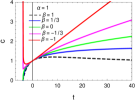
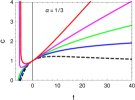
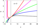
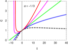
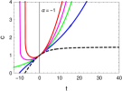
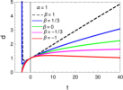
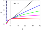
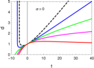
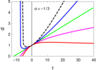
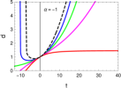
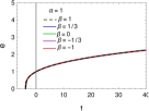
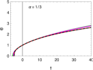
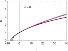
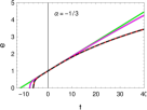
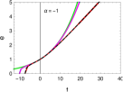
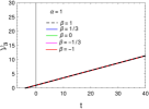
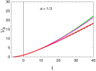
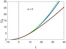
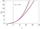
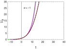
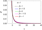
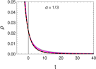
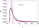
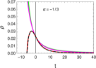
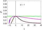
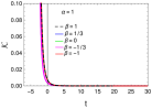
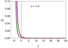
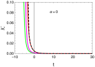
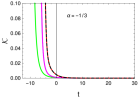
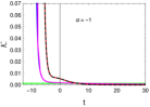
Figure 1: Plots of $c$, $d$, $e$, ${\cal V}_{3}$, $\rho$ and $\mathcal{K}$ for $\alpha,\beta=0,\pm 1/3,\pm 1$ and $n=0$. Each column is for the same value of $\alpha$. Values of $\beta$ are distinguished by color.

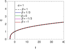
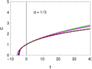
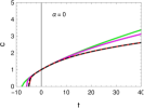
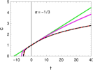
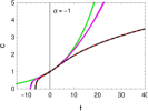
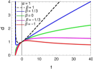
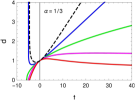
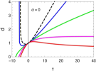
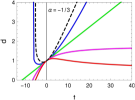
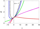
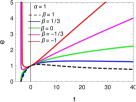
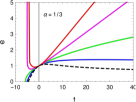
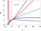
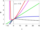
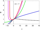
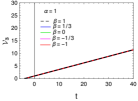
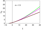
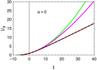
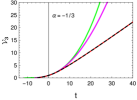
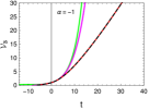
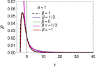
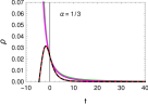
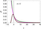
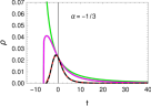
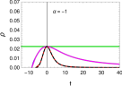
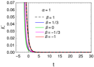
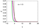
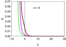
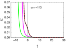
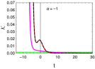
Figure 2: Plots of $c$, $d$, $e$, ${\cal V}_{3}$, $\rho$ and $\mathcal{K}$ for $\alpha,\beta=0,\pm 1/3,\pm 1$ and $n=1$. Each column is for the same value of $\alpha$. Values of $\beta$ are distinguished by color.

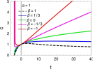
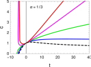
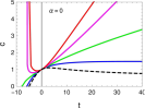
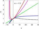
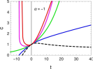
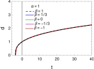
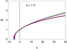
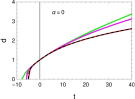
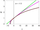
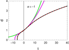
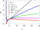
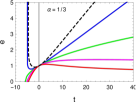
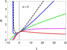
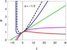
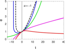
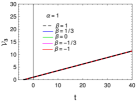
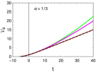
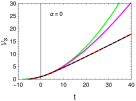
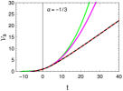
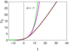
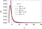
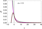
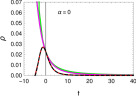
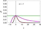
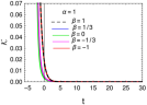
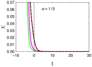
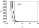
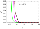
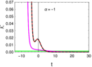
Figure 3: Plots of $c$, $d$, $e$, ${\cal V}_{3}$, $\rho$ and $\mathcal{K}$ for $\alpha,\beta=0,\pm 1/3,\pm 1$ and $n=-1$. Each column is for the same value of $\alpha$. Values of $\beta$ are distinguished by color.

III.2 Energy density $\rho$

The energy density $\rho$ in the Friedmann universe always diverges at the moment of big bang ($t\to t_{s}$) and decreases afterwards monotonically for $\alpha>-1$. It remains constant in time for the de Sitter case $\alpha=-1$.

For $\beta\neq 0$, however, we observe some cases where, unlike in the Friedmann universe, $\rho$ does not diverge as $t\to t_{s}$; $\rho$ increases from zero at the early stage, reaches a maximum value and then starts to decrease in time (see Figs. 1-3).

III.3 Kretschmann scalar $\mathcal{K}$

In the previous subsections, we found that the energy density $\rho$ does not necessarily diverge even though the three-volume density ${\cal V}_{3}$ vanishes at $t=t_{s}$. It is therefore useful to evaluate the curvature invariants to lookup the nature of the spacetime at $t=t_{s}$. The Kretschmann scalar is given by

$$\mathcal{K}=R^{\mu\nu\rho\sigma}R_{\mu\nu\rho\sigma}=\frac{(1/9216)}{(1+3n^{2})^{2}u^{\sqrt{3}}v^{\sqrt{3}}}\left(Y_{1}u^{4s_{1}}+Y_{2}u^{3s_{1}}v^{s_{2}}+Y_{3}u^{2s_{1}}v^{2s_{2}}+Y_{4}u^{s_{1}}v^{3s_{2}}+Y_{5}v^{4s_{2}}\right),$$ (30)

where

$$Y_{1} = A_{2}^{4}\left[\bar{n}_{2}^{4}X_{1}-\bar{n}_{1}\bar{n}_{2}^{3}X_{2}+\bar{n}_{1}^{2}\bar{n}_{2}^{2}X_{3}-\bar{n}_{1}^{3}\bar{n}_{2}X_{4}+\bar{n}_{1}^{4}X_{5}\right]$$

$$Y_{2} = -A_{1}A_{2}^{3}\left[4n_{2}\bar{n}_{2}^{3}X_{1}-(n_{1}\bar{n}_{2}+3\bar{n}_{1}n_{2})\bar{n}_{2}^{2}X_{2}+2(n_{1}\bar{n}_{2}+\bar{n}_{1}n_{2})\bar{n}_{1}\bar{n}_{2}X_{3}-(3n_{1}\bar{n}_{2}+\bar{n}_{1}n_{2})\bar{n}_{1}^{2}X_{4}+4n_{1}\bar{n}_{1}^{3}X_{5}\right]$$

$$Y_{3} = A_{1}^{2}A_{2}^{2}\left[6n_{2}^{2}\bar{n}_{2}^{2}X_{1}-3(n_{1}\bar{n}_{2}+\bar{n}_{1}n_{2})n_{2}\bar{n}_{2}X_{2}+(n_{1}^{2}\bar{n}_{2}^{2}+4n_{1}\bar{n}_{1}n_{2}\bar{n}_{2}+n_{2}^{2}\bar{n}_{1}^{2})X_{3}-3(n_{1}\bar{n}_{2}+\bar{n}_{1}n_{2})n_{1}\bar{n}_{1}X_{4}\right.$$

$$\left.+6n_{1}^{2}\bar{n}_{1}^{2}X_{5}\right]$$

$$Y_{4} = -A_{1}^{2}A_{2}\left[4n_{2}^{3}\bar{n}_{2}X_{1}-(3n_{1}\bar{n}_{2}+\bar{n}_{1}n_{2})n_{2}^{2}X_{2}+2(n_{1}\bar{n}_{2}+\bar{n}_{1}n_{2})n_{1}n_{2}X_{3}-(n_{1}\bar{n}_{2}+3\bar{n}_{1}n_{2})n_{1}^{2}X_{4}+4n_{1}^{3}\bar{n}_{1}X_{5}\right]$$

$$Y_{5} = A_{1}^{4}\left[n_{2}^{4}X_{1}-n_{1}n_{2}^{3}X_{2}+n_{1}^{2}n_{2}^{2}X_{3}-n_{1}^{3}n_{2}X_{4}+n_{1}^{4}X_{5}\right]$$

and

$$X_{1} = (1+3n)^{2}\left[7+2\alpha+3\alpha^{2}+8(1+n)\beta+8(1+3n^{2})\beta^{2}\right]$$

$$X_{2} = 8(1+3n)\left[1-6n+2\alpha+3\alpha^{2}+4(1-n)\beta+8(1+3n^{2})\beta^{2}\right]$$

$$X_{3} = 6\left[5+27n^{2}+6(1-n^{2})\alpha+9(1-n^{2})\alpha^{2}-8n(5+3n^{2})\beta+24(1-n^{2})(1+3n^{2})\beta^{2}\right]$$

$$X_{4} = 8(1-3n)\left[1+6n+2\alpha+3\alpha^{2}-4(1+n)\beta+8(1+3n^{2})\beta^{2}\right]$$

$$X_{5} = (1-3n)^{2}\left[7+2\alpha+3\alpha^{2}-8(1-n)\beta+8(1+3n^{2})\beta^{2}\right]$$

In the limit $t\to t_{s}$, one of the terms in Eq. (30) dominates. The nature of $\mathcal{K}$ in this limit depends on this dominating term. Note that, for $n=-1/3$, $Y_{1}=0$ and $Y_{2}=0$ as $X_{1}=0$, $X_{2}=0$ and $\bar{n}_{1}=0$. Therefore, the dominating term in this case is one of $Y_{3}$, $Y_{4}$ and $Y_{5}$. On the other hand , for $n=1/3$, $Y_{4}=0$ and $Y_{5}=0$ as $X_{4}=0$, $X_{5}=0$ and $n_{2}=0$. Therefore, the dominating term in this is one of $Y_{1}$, $Y_{2}$ and $Y_{3}$. As discussed in the previous section, for $n=\pm 1/3$, two of the effective pressures in the diagonal energy-momentum tensor become equal and the solution becomes equivalent to the one obtained in Ref. Cho:2022rgs . As shown in Ref. Cho:2022rgs , $\mathcal{K}$ in these cases does not always diverge, but is finite as $t\to t_{s}$ for some values of $\alpha$ and $\beta$.

On the other hand, for $n\neq\pm 1/3$, all the effective pressures are different, and none of the coefficients $Y_{1}$, $Y_{2}$, $Y_{4}$ and $Y_{5}$ is zero. Therefore, the dominating term and hence the nature of $\mathcal{K}$ as $t\to t_{s}$ is different from the ones for $n=\pm 1/3$. For $n=0,\pm 1$, we have plotted ${\cal K}$ in Figs. 1-3. Note that, unlike the results presented in Ref. Cho:2022rgs for $n=\pm 1/3$, $\mathcal{K}$ for $n=0,\pm 1$ always diverges and hence the solution is always singular. We will see this also later when we present the nature of $\mathcal{K}$ as $t\to t_{s}$ for arbitrary values of $n$, $\alpha$ and $\beta$.

III.4 $\rho(t_{s})$ & $\mathcal{K}(t_{s})$

In order to examine the nature of the spacetime at $t\to t_{s}$ for arbitrary $n$, $\alpha$ and $\beta$, we investigate the the behaviour of $\rho$ and $\mathcal{K}$ in the limit $t\to t_{s}$. Considering the signatures of the terms in the integrand, the $v$-solution for Class G in Eq. (20) is classified into four cases,
(i) G1: $\beta<0\;\&\;s_{2}=\sqrt{3}(1-\alpha)+2\sqrt{1+3n^{2}}\beta>0$,
(ii) G2: $\beta<0\;\&\;s_{2}=\sqrt{3}(1-\alpha)+2\sqrt{1+3n^{2}}\beta<0$,
(iii) G3: $\beta>0\;\&\;s_{1}=\sqrt{3}(1-\alpha)-2\sqrt{1+3n^{2}}\beta>0$,
(iv) G4: $\beta>0\;\&\;s_{1}=\sqrt{3}(1-\alpha)-2\sqrt{1+3n^{2}}\beta<0$.
The behaviour of ${\cal V}_{3}$ as well as $\rho$ and $\mathcal{K}$ in the limit $t\to t_{s}$ is obtained in Appendix B. In this limit, $\rho$ and $\mathcal{K}$ behave as [see Eqs. (68) and (69)]

$$\rho\sim\left\{\begin{array}[]{ll}\frac{1}{(t-t_{s})^{[\sqrt{3}(1+\alpha)+2\sqrt{1+3n^{2}}\beta]/\sqrt{3}}}&(\mbox{G1 and G2})\\ \frac{1}{(t-t_{s})^{[\sqrt{3}(1+\alpha)-2\sqrt{1+3n^{2}}\beta]/\sqrt{3}}}&(\mbox{G3 and G4})\end{array}\right.,$$ (31)

$$\mathcal{K}\sim\left\{\begin{array}[]{lllll}\frac{1}{(t-t_{s})^{4}}&\mbox{for $n\neq\pm 1/3$}\quad(\mbox{G1-G4})\\ \frac{1}{(t-t_{s})^{4}}&\mbox{for $n=-1/3$}\quad(\mbox{G1 and G2})\\ \frac{1}{(t-t_{s})^{2(1+\alpha-4\beta/3)}}&\mbox{for $n=-1/3$}\quad(\mbox{G3 and G4})\\ \frac{1}{(t-t_{s})^{2(1+\alpha+4\beta/3)}}&\mbox{for $n=1/3$}\quad(\mbox{G1 and G2})\\ \frac{1}{(t-t_{s})^{4}}&\mbox{for $n=1/3$}\quad(\mbox{G3 and G4})\end{array}\right..$$ (32)

The behaviour of $\rho(t_{s})$ and ${\cal K}(t_{s})$ can be characterized by the regions in the $\alpha$-$\beta$ plane in Fig. 4. The regions are split by two lines S1 ($\sqrt{3}(1+\alpha)+2\sqrt{1+3n^{2}}\beta=0$) and S2 ($\sqrt{3}(1+\alpha)-2\sqrt{1+3n^{2}}\beta=0$).

1) In the region below S1: (i) $\rho(t_{s})={\cal K}(t_{s})=0$ for $n=1/3$, (ii) $\rho(t_{s})=0$ but ${\cal K}(t_{s})$ diverges for all other values of $n$.

2) On S1: (i) $\rho(t_{s})$ and ${\cal K}(t_{s})$ are finite for $n=1/3$, (ii) $\rho(t_{s})$ is finite but ${\cal K}(t_{s})$ diverges for all other values of $n$.

3) In the region between S1 and S2: both $\rho(t_{s})$ and ${\cal K}(t_{s})$ diverge for all values of $n$.

4) On S2: (i) $\rho(t_{s})$ and ${\cal K}(t_{s})$ are finite for $n=-1/3$, (ii) $\rho(t_{s})$ is finite but ${\cal K}(t_{s})$ diverges for all other values of $n$.

5) In the region above S2: (i) $\rho(t_{s})={\cal K}(t_{s})=0$ for $n=-1/3$, (ii) $\rho(t_{s})=0$ but ${\cal K}(t_{s})$ diverges for all other values of $n$.

Therefore, in the region $\sqrt{3}(1+\alpha)-2\sqrt{1+3n^{2}}|\beta|\leq 0$, the energy density is finite for all the values of $n$, whereas the Kretschmann scalar is finite only for $n=\pm 1/3$. Therefore, for $n\neq\pm 1/3$, the solution is always singular. The initial singularity can only be removed on S1 and in the region below for $n=1/3$, and on S2 and in the region above for $n=-1/3$.

Let us discuss the energy conditions. The standard energy conditions (poisson, ) for the diagonal energy-momentum tensor in Eq. (7) turn out to be
(a) Weak Energy Condition (WEC):

$$\rho\geq 0,\;\;\rho+p+(n+1)\sigma>0,\;\;\rho+p+(n-1)\sigma>0,\;\;\rho+p-2n\sigma>0$$

$$\Rightarrow \rho\geq 0,\;\;1+\alpha+(n+1)\beta>0,\;\;1+\alpha+(n-1)\beta>0\;\;1+\alpha-2n\beta>0.$$

(b) Null Energy Condition (NEC):

$$\rho+p+(n+1)\sigma\geq 0,\;\;\rho+p+(n-1)\sigma\geq 0,\;\;\rho+p-2n\sigma\geq 0$$

$$\Rightarrow 1+\alpha+(n+1)\beta\geq 0,\;\;1+\alpha+(n-1)\beta\geq 0\;\;1+\alpha-2n\beta\geq 0.$$

(c) Strong Energy Condition (SEC):

$$\rho+p+(n+1)\sigma\geq 0,\;\;\rho+p+(n-1)\sigma\geq 0,\;\;\rho+p-2n\sigma\geq 0,\;\;\rho+3p\geq 0$$

$$\Rightarrow 1+\alpha+(n+1)\beta\geq 0,\;\;1+\alpha+(n-1)\beta\geq 0\;\;1+\alpha-2n\beta\geq 0,\;\;1+3\alpha\geq 0.$$

(d) Dominant Energy Condition (DEC):

$$\rho\geq 0,\;\;\rho\geq|p+(n+1)\sigma|,\;\;\rho\geq|p+(n-1)\sigma|,\;\;\rho\geq|p-2n\sigma|$$

$$\Rightarrow \rho\geq 0,\;\;1-|\alpha+(n+1)\beta|\geq 0,\;\;1-|\alpha+(n-1)\beta|\geq 0\;\;1-|\alpha-2n\beta|\geq 0.$$

Here, we have used the equations of state given in Eq. (11). In the region enclosed by the red dotted lines in Fig. 4 (rhombus for $n=0$ and parallelogram for $n\neq 0$), the WEC, NEC and DEC are satisfied. The SEC is satisfied also in this region if $\alpha\geq-1/3$. Outside of this enclosed region, at least one energy condition is violated. It is to be noted that this energy condition violating region consists of four triangles. Inside the two left triangles, all the energy conditions are violated, whereas only the DEC is violated inside the two right triangles. It is to be noted also that, for $n=\pm 1/3$, the region where the singularity can be removed belongs to the region where all the energy conditions are violated ($n=-1/3$: upper triangle, $n=+1/3$: lower triangle).

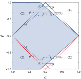
(a) $n=0$

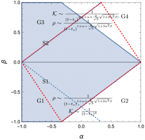
(b) $n=-1/3$

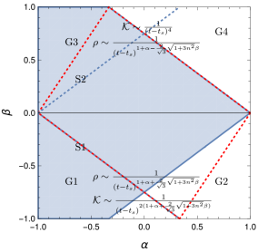
(c) $n=1/3$

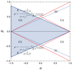
(d) $n=\pm 1$

Figure 4: Diagram for $\rho$ and $\mathcal{K}$ at $t\to t_{s}$ in $\alpha$-$\beta$ plane. Class G is split into four regions by G1-G4. The shaded region ($\sqrt{3}(1-\alpha)-2\sqrt{1+3n^{2}}|\beta|>0$) consists of G1 and G3 divided by $\beta=0$, and the unshaded region ($\sqrt{3}(1-\alpha)-2\sqrt{1+3n^{2}}|\beta|<0$) consists of G2 and G4. The blue dotted lines S1 and S2 represent $\sqrt{3}(1+\alpha)+2\sqrt{1+3n^{2}}\beta=0$ and $\sqrt{3}(1+\alpha)-2\sqrt{1+3n^{2}}\beta=0$, respectively.

IV Late time behaviour

We now analyse the late-time (large $t$) behaviour of the solutions for different classes separately. The results are summarized in Fig. 5.

Class G: General Class

The late-time behaviour of the solution in this class is obtained in Appendix C. As $t\to\infty$, the three-volume and the energy density behave as (see Eqs. (74) and (75))

$${\cal V}_{3}\sim\left\{\begin{array}[]{ll}t^{\frac{6(1-\alpha)}{3(1-\alpha^{2})+4(1+3n^{2})\beta^{2}}}&(\mbox{G1 and G3})\\ t&(\mbox{G2 and G4})\end{array}\right.,$$ (33)

and

$$\rho\sim\left\{\begin{array}[]{ll}\frac{1}{t^{2}}&(\mbox{G1 and G3})\\ \frac{1}{t^{[\sqrt{3}(1+\alpha)+2\sqrt{1+3n^{2}}|\beta|]/\sqrt{3}}}&(\mbox{G2 and G4})\end{array}\right..$$ (34)

It is to be noted that ${\cal V}_{3}$ diverges and $\rho$ vanishes as $t\to\infty$.

Class A ($[\sqrt{3}(1-\alpha)+2\sqrt{1+3n^{2}}\beta]=0$) and Class B ($[\sqrt{3}(1-\alpha)-2\sqrt{1+3n^{2}}\beta]=0$)

For these classes, it is difficult to obtain the late-time behaviour of the solution directly from Eqs. (22) and (24). However, since Class A is the border of G1 and G2, and Class B is the same of G3 and G4 (see Fig. 5), we can find out the late-time behaviour of ${\cal V}_{3}$ and $\rho$ by putting $\left[\sqrt{3}(1-\alpha)-2\sqrt{1+3n^{2}}|\beta|\right]=0$ in Eqs. (33) and (34). This gives

$${\cal V}_{3}\sim t,\qquad\rho\sim\frac{1}{t^{2}}.$$ (35)

Class C: $\beta=0$

(i) FRW universe: For this class, at large $t$, we have, from Eq. (28),

$$c=d\sim\left\{\begin{array}[]{lr}e^{\frac{A_{2}}{2\sqrt{3}}t}&(\alpha=-1)\\ t^{\frac{2}{3(1+\alpha)}}&(\alpha\neq-1)\end{array}\right..$$ (36)

Therefore, ${\cal V}_{3}$ and $\rho$ at large $t$ are given by

$${\cal V}_{3}\sim\left\{\begin{array}[]{lr}e^{\frac{\sqrt{3}A_{2}}{2}t}&(\alpha=-1)\\ t^{\frac{2}{(1+\alpha)}}&(\alpha\neq-1)\end{array}\right.,\qquad\rho\sim\left\{\begin{array}[]{lr}{\rm const.}&(\alpha=-1)\\ \frac{1}{t^{2}}&(\alpha\neq-1)\end{array}\right..$$ (37)

Class C corresponds to the horizontal axis in Fig. 5.

(ii) Non-FRW universe: The solution for this class is given by Eqs. (25) and (26). However, we find that the late-time behaviours of ${\cal V}_{3}$ and $\rho$ in this class remains the same as that in Class C-(i).

The late-time behaviours of ${\cal V}_{3}$ and $\rho$ are summarized in Fig. 5 for $n=0,\pm 1$. In comparison to those in FRW, $\rho$ evolves in the same manner and ${\cal V}_{3}$ exhibits slower expansion in the shaded region (regions G1 and G3), whereas, in the unshaded region (regions G2 and G4), $\rho$ decreases faster and ${\cal V}_{3}$ again exhibits slower expansion. Therefore, with off-diagonal stress, the expansion of ${\cal V}_{3}$ is slower, and $\rho$ decreases more rapidly (at most equally) compared with the FRW universe.

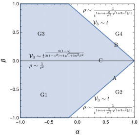
(a) $n=0$

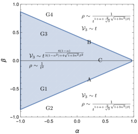
(b) $n=\pm 1$

Figure 5: Diagram for ${\cal V}_{3}$ and $\rho$ at large $t$ in $\alpha$-$\beta$ plane. The lower border between the shaded and the unshaded regions corresponds to Class A, and the upper border to Class B. The solid horizontal line between G1 and G3 to Class C ($\beta=0$: FRW). Considering the power in $t$, $\rho$ evolves in the same manner with that of FRW in the shaded region, and decreases faster than that of FRW in the unshaded region. ${\cal V}_{3}$ increases slower than that of FRW in all regions.

V Conclusions

We have investigated in detail the effect of the off-diagonal stress tensor (shear viscosity) on the evolution of spacetime. We have solved the Eintein’s equation and have obtained exact solutions. The shear viscosity part has diagonal as well as off-diagonal components. Under a certain condition ($p_{1}=p_{2}=p_{3}$), we find that the diagonal component $\sigma_{1}$ is proportional to the off-diagonal component $\sigma$, i.e., $\sigma_{1}=n\sigma$, $n$ being a constant. For $n=\pm 1/3$, the solution reduces to our earlier results obtained in Ref. Cho:2022rgs . (The energy-momentum tensor as well as the metric can be put into diagonal forms through a suitable coordinate transformation).

We considered two equation of states, $p=\alpha\rho$ and $\sigma=\beta\rho$, and solved the Einstein’s equation for the range $-1\leq\alpha,\beta\leq 1$. Depending on the values of the parameters $\alpha$ and $\beta$, the solution was classified into several classes. We analysed the early-time and the late-time behaviour of the solution.

The three-volume density ${\cal V}_{3}$ vanishes at the initial moment $t_{s}$ for all the classes except for the pure de Sitter ($\alpha=-1,\beta=0$). ${\cal V}_{3}$ increases monotonically afterwards. At late times, ${\cal V}_{3}$ increases slower than that of FRW. The evolution pattern of $\rho$, on the other hand, depends on the parameters. In the parameter region $\sqrt{3}(1+\alpha)-2\sqrt{1+3n^{2}}|\beta|\leq 0$, $\rho$ is finite at $t_{s}$. Outside of this region, $\rho$ diverges at $t_{s}$ and drops afterwards as the usual FRW universe ($\beta=0$). At late times, $\rho$ drops faster than, or at most equal to that in the Friedmann universe considering the power of $t$-dependence.

For $n\neq\pm 1/3$, the solution is always singular as the Kretshmann scalar (${\cal K}$) always diverges at the initial moment $t_{s}$ in these cases. For $n=\pm 1/3$, however, the initial big-bang singularity can be removed for some parameter ranges (see Ref. Cho:2022rgs for more details of these cases). For this case, the evolution along two spatial directions are equal which is Bianchi type-VII. For $n\neq\pm 1/3$, the evolution along all three directions are different which is Bianchi type-I. Therefore, the latter is more anisotropic (less symmetry) than the former, and the effect of this is reflected in the early-time behaviour of the solution; the solution is always singular for $n\neq\pm 1/3$, whereas it can be either singular or non-singular for $n=\pm 1/3$.

Appendix A Integrating the field equations

With Eqs. (11) and (8), Eqs. (9) and (10) can be written as

$$2(1+n)\frac{\ddot{c}}{c}+(1+3n)(\alpha+n)\frac{\dot{c}^{2}}{c^{2}}+2(1+2\alpha-3n^{2})\frac{\dot{c}}{c}\frac{\dot{d}}{d}+(1-3n)(\alpha-n)\frac{\dot{d}^{2}}{d^{2}}+2(1-n)\frac{\ddot{d}}{d}=0,$$ (38)

$$2\frac{\ddot{c}}{c}+(1+3n)(1+2\beta)\frac{\dot{c}^{2}}{c^{2}}-(6n-8\beta)\frac{\dot{c}}{c}\frac{\dot{d}}{d}-(1-3n)(1-2\beta)\frac{\dot{d}^{2}}{d^{2}}-2\frac{\ddot{d}}{d}=0.$$ (39)

Now multiplying Eq. (39) by $\sqrt{1+3n^{2}}/\sqrt{3}$ and then adding with Eq. (38), we obtain

$$\frac{d}{dt}\left[c^{q_{1}}d^{q_{2}}\left(n_{1}d\dot{c}+n_{2}c\dot{d}\right)\right]=0,$$ (40)

where

$$q_{1}=\frac{1+3n}{2n_{1}}\left[\sqrt{3}(\alpha+n)+\sqrt{1+3n^{2}}(1+2\beta)\right],$$ (41)

$$q_{2}=\frac{1-3n}{2n_{2}}\left[\sqrt{3}(\alpha-n)-\sqrt{1+3n^{2}}(1-2\beta)\right],$$ (42)

$$n_{1}=\sqrt{3}(1+n)+\sqrt{1+3n^{2}},\quad n_{2}=\sqrt{3}(1-n)-\sqrt{1+3n^{2}}.$$ (43)

Integrating this equation, we get

$$n_{1}d\dot{c}+n_{2}c\dot{d}=\frac{A_{2}}{c^{q_{1}}d^{q_{2}}},$$ (44)

where $A_{2}$ is an integration constant. The conservation equation turns out to be

$$\dot{\rho}+\frac{3}{2}\left[(1+n)\frac{\dot{c}}{c}+(1-n)\frac{\dot{d}}{d}\right](\rho+p)-(1+3n^{2})\left(\frac{\dot{c}}{c}-\frac{\dot{d}}{d}\right)\sigma=0,$$ (45)

which, after using Eq. (11), can be integrated to obtain

$$\rho=\frac{A_{0}}{c^{\frac{3}{2}(1+n)(1+\alpha)-(1+3n^{2})\beta}d^{\frac{3}{2}(1-n)(1+\alpha)+(1+3n^{2})\beta}},$$ (46)

where $A_{0}$ is an integration constant. Equation (8), then, can be written as

$$\frac{1}{4c^{2}d^{2}}\left(n_{1}d\dot{c}+n_{2}c\dot{d}\right)\left(\bar{n}_{1}d\dot{c}+\bar{n}_{2}c\dot{d}\right)=\frac{A_{0}}{c^{\frac{3}{2}(1+n)(1+\alpha)-(1+3n^{2})\beta}d^{\frac{3}{2}(1-n)(1+\alpha)+(1+3n^{2})\beta}},$$ (47)

where

$$\bar{n}_{1}=\sqrt{3}(1+n)-\sqrt{1+3n^{2}},\quad\bar{n}_{2}=\sqrt{3}(1-n)+\sqrt{1+3n^{2}}.$$ (48)

Using Eq. (44), Eq. (47) can be rewritten as

$$\bar{n}_{1}d\dot{c}+\bar{n}_{2}c\dot{d}=\frac{A_{1}}{c^{\bar{q}_{1}}d^{\bar{q}_{2}}},$$ (49)

where $A_{0}=A_{1}A_{2}/4$ and

$$\bar{q}_{1}=\frac{3}{2}(1+n)(1+\alpha)-(1+3n^{2})\beta-2-q_{1},$$ (50)

$$\bar{q}_{2}=\frac{3}{2}(1-n)(1+\alpha)+(1+3n^{2})\beta-2-q_{2}.$$ (51)

Introducing new variables, $u=c^{\bar{n}_{1}}d^{\bar{n}_{2}}$ and $v=c^{n_{1}}d^{n_{2}}$, Eqs. (49) and (44) can be rewritten as

$$\frac{\dot{u}}{u}=\frac{A_{1}}{u^{-\frac{n_{2}(\bar{q}_{1}+1)}{n_{1}\bar{n}_{2}-\bar{n}_{1}n_{2}}+\frac{n_{1}(\bar{q}_{2}+1)}{n_{1}\bar{n}_{2}-\bar{n}_{1}n_{2}}}v^{\frac{\bar{n}_{2}(\bar{q}_{1}+1)}{n_{1}\bar{n}_{2}-\bar{n}_{1}n_{2}}-\frac{\bar{n}_{1}(\bar{q}_{2}+1)}{n_{1}\bar{n}_{2}-\bar{n}_{1}n_{2}}}},$$ (52)

$$\frac{\dot{v}}{v}=\frac{A_{2}}{u^{-\frac{n_{2}(q_{1}+1)}{n_{1}\bar{n}_{2}-\bar{n}_{1}n_{2}}+\frac{n_{1}(q_{2}+1)}{n_{1}\bar{n}_{2}-\bar{n}_{1}n_{2}}}v^{\frac{\bar{n}_{2}(q_{1}+1)}{n_{1}\bar{n}_{2}-\bar{n}_{1}n_{2}}-\frac{\bar{n}_{1}(q_{2}+1)}{n_{1}\bar{n}_{2}-\bar{n}_{1}n_{2}}}}.$$ (53)

Introducing

$$s_{1}=-\frac{n_{2}(\bar{q}_{1}-q_{1})}{n_{1}\bar{n}_{2}-\bar{n}_{1}n_{2}}+\frac{n_{1}(\bar{q}_{2}-q_{2})}{n_{1}\bar{n}_{2}-\bar{n}_{1}n_{2}}=\frac{1}{4}\left[\sqrt{3}(1-\alpha)-2\sqrt{1+3n^{2}}\beta\right],$$ (54)

$$s_{2}=-\frac{\bar{n}_{2}(\bar{q}_{1}-q_{1})}{n_{1}\bar{n}_{2}-\bar{n}_{1}n_{2}}+\frac{\bar{n}_{1}(\bar{q}_{2}-q_{2})}{n_{1}\bar{n}_{2}-\bar{n}_{1}n_{2}}=\frac{1}{4}\left[\sqrt{3}(1-\alpha)+2\sqrt{1+3n^{2}}\beta\right],$$ (55)

Eqs. (52) and (53) can be written as

$$\frac{\dot{u}}{u}=\frac{A_{1}}{u^{\sqrt{3}/4}v^{\sqrt{3}/4-s_{2}}},$$ (56)

$$\frac{\dot{v}}{v}=\frac{A_{2}}{u^{\sqrt{3}/4-s_{1}}v^{\sqrt{3}/4}}.$$ (57)

In terms of $u$ and $v$, $\rho$ can be written as

$$\rho=\frac{(A_{1}A_{2}/4)}{u^{\sqrt{3}/2-s_{1}}v^{\sqrt{3}/2-s_{2}}}.$$ (58)

So, all the field equations reduces to Eqs. (56), (57) and (58).

Appendix B Early-time behaviour

Here, we investigate the behaviour of the solutions in the limit of $t\to t_{s}$. At $t=0$, we imposed the initial conditions, $c(0)=d(0)=1$ and $\dot{c}(0)=\dot{d}(0)$, which are equivalent to $u(0)=v(0)=1$ and $\dot{u}(0)=\dot{v}(0)$. Using these conditions, we obtain $A_{2}=A_{1}$ from Eq. (18) and $A_{3}=(1-{s_{1}}/{s_{2}})=\sqrt{1+3n^{2}}\beta/{s_{2}}$ from Eq. (19). Now depending on the signatures of the terms in the integrand, the $v$-solution for Class G in Eq. (20) can be classified into four cases,

$$t=\left\{\begin{array}[]{lr}\frac{1}{A_{2}}\int_{1}^{v}v^{\sqrt{3}/4-1}\left[\frac{s_{1}}{s_{2}}\left(v^{s_{2}}-v_{*}^{s_{2}}\right)\right]^{\frac{\sqrt{3}}{4s_{1}}-1}dv&[\mbox{G1: }\beta<0\;\&\;s_{2}=\sqrt{3}(1-\alpha)+2\sqrt{1+3n^{2}}\beta>0]\\ \frac{1}{A_{2}}\int_{1}^{v}v^{\sqrt{3}/4-1}\left[\frac{s_{1}}{|s_{2}|}\left(-v^{s_{2}}+v_{*}^{s_{2}}\right)\right]^{\frac{\sqrt{3}}{4s_{1}}-1}dv&[\mbox{G2: }\beta<0\;\&\;s_{2}=\sqrt{3}(1-\alpha)+2\sqrt{1+3n^{2}}\beta<0]\\ \frac{1}{A_{2}}\int_{1}^{v}v^{\sqrt{3}/4-1}\left[\frac{s_{1}}{s_{2}}\left(v^{s_{2}}+v_{*}^{s_{2}}\right)\right]^{\frac{\sqrt{3}}{4s_{1}}-1}dv&[\mbox{G3: }\beta>0\;\&\;s_{1}=\sqrt{3}(1-\alpha)-2\sqrt{1+3n^{2}}\beta>0]\\ \frac{1}{A_{2}}\int_{1}^{v}v^{\sqrt{3}/4-1}\left[\frac{|s_{1}|}{s_{2}}\left(-v^{s_{2}}+v_{*}^{s_{2}}\right)\right]^{\frac{\sqrt{3}}{4s_{1}}-1}dv&[\mbox{G4: }\beta>0\;\&\;s_{1}=\sqrt{3}(1-\alpha)-2\sqrt{1+3n^{2}}\beta<0]\end{array}\right.,$$ (59)

where $v_{*}=\left(\sqrt{1+3n^{2}}|\beta|/|s_{1}|\right)^{1/s_{2}}$. Note that, for $-1\leq\alpha\leq 1$, we have $\sqrt{3}(1-\alpha)-2\sqrt{1+3n^{2}}\beta>0$ ($s_{1}>0$) if $\beta<0$, and $\sqrt{3}(1-\alpha)+2\sqrt{1+3n^{2}}\beta>0$ ($s_{2}>0$) if $\beta>0$. As $t\to t_{s}$, $v$ approaches to its minimum value; $v\to v_{*}$ for G1 and G2, and $v\to 0$ for G3 and G4. We split the integration range into two parts as

$$\int_{1}^{v}[\cdots]dv=\left(\int_{1}^{v_{s}}+\int_{v_{s}}^{v}\right)[\cdots]dv,\quad\mbox{where }\int_{1}^{v_{s}}[\cdots]dv\equiv t_{s}\mbox{ and }v_{s}=\left\{\begin{array}[]{l}\mbox{$v_{*}$ (for G1 and G2)}\\ \mbox{$0$ (for G3 and G4)}\end{array}\right..$$ (60)

Therefore, Eq. (59) can be rewritten as

$$t-t_{s}=\left\{\begin{array}[]{lr}\frac{1}{A_{2}}\int_{0}^{v}v^{\sqrt{3}/4-1}\left[\frac{s_{1}}{s_{2}}\left(v^{s_{2}}-v_{*}^{s_{2}}\right)\right]^{\frac{\sqrt{3}}{4s_{1}}-1}dv&(\mbox{G1})\\ \frac{1}{A_{2}}\int_{0}^{v}v^{\sqrt{3}/4-1}\left[\frac{s_{1}}{|s_{2}|}\left(-v^{s_{2}}+v_{*}^{s_{2}}\right)\right]^{\frac{\sqrt{3}}{4s_{1}}-1}dv&(\mbox{G2})\\ \frac{1}{A_{2}}\int_{v_{*}}^{v}v^{\sqrt{3}/4-1}\left[\frac{s_{1}}{s_{2}}\left(v^{s_{2}}+v_{*}^{s_{2}}\right)\right]^{\frac{\sqrt{3}}{4s_{1}}-1}dv&(\mbox{G3})\\ \frac{1}{A_{2}}\int_{v_{*}}^{v}v^{\sqrt{3}/4-1}\left[\frac{|s_{1}|}{s_{2}}\left(-v^{s_{2}}+v_{*}^{s_{2}}\right)\right]^{\frac{\sqrt{3}}{4s_{1}}-1}dv&(\mbox{G4})\end{array}\right..$$ (61)

We now perform the Taylor expansion about $v=v_{*}$ and keep the leading order of the term in the parentheses of the integrand for G1 and G2. For G3 and G4, we set $v=0$ in the parentheses of the integrand and get the leading order. After doing so, the integration gives, in the limit of $t\to t_{s}$,

$$v\sim\left\{\begin{array}[]{ll}v_{*}+{\rm const.}\times(t-t_{s})^{4s_{1}/\sqrt{3}}&(\mbox{G1 and G2})\\ (t-t_{s})^{4/\sqrt{3}}&(\mbox{G3 and G4})\end{array}\right..$$ (62)

Using $v$, we obtain $u$ from Eq. (19),

$$u\sim\left\{\begin{array}[]{ll}(t-t_{s})^{4/\sqrt{3}}&(\mbox{G1 and G2})\\ u_{*}+{\rm const.}\times(t-t_{s})^{4s_{2}/\sqrt{3}}&(\mbox{G3 and G4})\end{array}\right.,$$ (63)

where $u_{*}=\left(|s_{1}|v_{*}^{s_{2}}/|s_{2}|\right)^{1/{s_{1}}}$. Note that the dependence of $c$ and $d$ on $(t-t_{s})$ can be obtained from the expressions

$$c=u^{-\frac{n_{2}}{n_{1}\bar{n}_{2}-\bar{n}_{1}n_{2}}}v^{\frac{\bar{n}_{2}}{n_{1}\bar{n}_{2}-\bar{n}_{1}n_{2}}},\quad d=u^{\frac{n_{1}}{n_{1}\bar{n}_{2}-\bar{n}_{1}n_{2}}}v^{-\frac{\bar{n}_{1}}{n_{1}\bar{n}_{2}-\bar{n}_{1}n_{2}}}.$$ (64)

We obtain, in the limit of $t\to t_{s}$,

$$c\sim\left\{\begin{array}[]{ll}(t-t_{s})^{-\frac{\sqrt{3}(1-n)-\sqrt{1+3n^{2}}}{3\sqrt{1+3n^{2}}}}&(\mbox{G1 and G2})\\ (t-t_{s})^{\frac{\sqrt{3}(1-n)+\sqrt{1+3n^{2}}}{3\sqrt{1+3n^{2}}}}&(\mbox{G3 and G4})\end{array}\right.,$$ (65)

$$d\sim\left\{\begin{array}[]{ll}(t-t_{s})^{\frac{\sqrt{3}(1+n)+\sqrt{1+3n^{2}}}{3\sqrt{1+3n^{2}}}}&(\mbox{G1 and G2})\\ (t-t_{s})^{-\frac{\sqrt{3}(1+n)-\sqrt{1+3n^{2}}}{3\sqrt{1+3n^{2}}}}&(\mbox{G3 and G4})\end{array}\right..$$ (66)

Therefore, the three-volume density behaves as

$${\cal V}_{3}\sim t-t_{s}\quad\mbox{(G1-G4)},$$ (67)

the energy density becomes

$$\rho\sim\left\{\begin{array}[]{ll}\frac{1}{(t-t_{s})^{[\sqrt{3}(1+\alpha)+2\sqrt{1+3n^{2}}\beta]/\sqrt{3}}}&(\mbox{G1 and G2})\\ \frac{1}{(t-t_{s})^{[\sqrt{3}(1+\alpha)-2\sqrt{1+3n^{2}}\beta]/\sqrt{3}}}&(\mbox{G3 and G4})\end{array}\right.,$$ (68)

and the Kretschmann scalar becomes

$$\mathcal{K}\sim\left\{\begin{array}[]{lllll}\frac{1}{(t-t_{s})^{4}}&\mbox{for $n\neq\pm 1/3$}\quad(\mbox{G1-G4})\\ \frac{1}{(t-t_{s})^{4}}&\mbox{for $n=-1/3$}\quad(\mbox{G1 and G2})\\ \frac{1}{(t-t_{s})^{2(1+\alpha-4\beta/3)}}&\mbox{for $n=-1/3$}\quad(\mbox{G3 and G4})\\ \frac{1}{(t-t_{s})^{2(1+\alpha+4\beta/3)}}&\mbox{for $n=1/3$}\quad(\mbox{G1 and G2})\\ \frac{1}{(t-t_{s})^{4}}&\mbox{for $n=1/3$}\quad(\mbox{G3 and G4})\end{array}\right..$$ (69)

Appendix C Late time behaviour

Here we obtain the late time behaviour of the Class G solution. We expect the integration in Eq. (59) to diverge as $t\to\infty$. For Class G1, G2 and G3, we have observed from our calculations that the integration diverges as $v\to\infty$. For the class G4, however, the integration diverges as $v\to v_{*}$.

At large $t$, the integrations in $v$ yield

$$v\sim\left\{\begin{array}[]{ll}t^{\frac{4[\sqrt{3}(1-\alpha)-2\sqrt{1+3n^{2}}\beta]}{3(1-\alpha^{2})+4(1+3n^{2})\beta^{2}}}&(\mbox{G1 and G3})\\ t^{4/\sqrt{3}}&(\mbox{G2})\\ v_{*}-{\rm const.}\times t^{-|\sqrt{3}(1-\alpha)-2\sqrt{1+3n^{2}}\beta|/\sqrt{3}}&(\mbox{G4})\end{array}\right..$$ (70)

Using $v$, we obtain $u$ from Eq. (19) at large $t$,

$$u\sim\left\{\begin{array}[]{ll}t^{\frac{4[\sqrt{3}(1-\alpha)+2\sqrt{1+3n^{2}}\beta]}{3(1-\alpha^{2})+4(1+3n^{2})\beta^{2}}}&(\mbox{G1 and G3})\\ u_{*}-{\rm const.}\times t^{-|\sqrt{3}(1-\alpha)+2\sqrt{1+3n^{2}}\beta|/\sqrt{3}}&(\mbox{G2})\\ t^{4/\sqrt{3}}&(\mbox{G4})\end{array}\right..$$ (71)

The late-time behaviour of $c$ and $d$, therefore, become

$$c\sim\left\{\begin{array}[]{ll}t^{\frac{2[1-\alpha-2(1-n)\beta]}{3(1-\alpha^{2})+4(1+3n^{2})\beta^{2}}}&(\mbox{G1 and G3})\\ t^{\frac{\sqrt{3}(1-n)+\sqrt{1+3n^{2}}}{3\sqrt{1+3n^{2}}}}&(\mbox{G2})\\ t^{-\frac{\sqrt{3}(1-n)-\sqrt{1+3n^{2}}}{3\sqrt{1+3n^{2}}}}&(\mbox{G4})\end{array}\right.,$$ (72)

$$d\sim\left\{\begin{array}[]{ll}t^{\frac{2[1-\alpha+2(1+n)\beta]}{3(1-\alpha^{2})+4(1+3n^{2})\beta^{2}}}&(\mbox{G1 and G3})\\ t^{-\frac{\sqrt{3}(1+n)-\sqrt{1+3n^{2}}}{3\sqrt{1+3n^{2}}}}&(\mbox{G2})\\ t^{\frac{\sqrt{3}(1+n)+\sqrt{1+3n^{2}}}{3\sqrt{1+3n^{2}}}}&(\mbox{G4})\end{array}\right.,$$ (73)

The three-volume density becomes

$${\cal V}_{3}\sim\left\{\begin{array}[]{ll}t^{\frac{6(1-\alpha)}{3(1-\alpha^{2})+4(1+3n^{2})\beta^{2}}}&(\mbox{G1 and G3})\\ t&(\mbox{G2 and G4})\end{array}\right..$$ (74)

The energy density becomes

$$\rho\sim\left\{\begin{array}[]{ll}\frac{1}{t^{2}}&(\mbox{G1 and G3})\\ \frac{1}{t^{[\sqrt{3}(1+\alpha)+2\sqrt{1+3n^{2}}|\beta|]/\sqrt{3}}}&(\mbox{G2 and G4})\end{array}\right..$$ (75)

Note that ${\cal V}_{3}$ diverges and $\rho$ vanishes as $t\to\infty$.

References

- (1) W. Misner, K. S. Thorne, and J. A. Wheeler, “Gravitation,” (Princeton University Press, USA, 2017).
- (2) C. W. Misner, “The Isotropy of the universe,” Astrophys. J. 151, 431-457 (1968) doi:10.1086/149448
- (3) J. M. Stewart, “Neutrino Viscosity in Cosmological Models,” Astrophysical Letters 2, 133-135 (1968).
- (4) J. M. Stewart, “Non-Equilibrium Processes in the Early Universe,” Monthly Notices of the Royal Astronomical Society 145, 347-356 (1969).
- (5) A. G. Doroshkevich, Ya. B. Zel’dovich, and I. D. Novikov, “Weakly Interacting Particles in the Anisotropic Cosmological Model ,” Soviet Phys. JETP 26, 408 (1968).
- (6) H. Noh and J. C. Hwang, “Second-order perturbations of the Friedmann world model,” Phys. Rev. D 69, 104011 (2004).
- (7) J. C. Hwang and H. Noh, “Second-order perturbations of cosmological fluids: Relativistic effects of pressure, multi-component, curvature, and rotation,” Phys. Rev. D 76, 103527 (2007).
- (8) J. C. Hwang, D. Jeong and H. Noh, “Gauge dependence of gravitational waves generated from scalar perturbations,” Astrophys. J. 842, no.1, 46 (2017).
- (9) C. Eckart, Phys. Rev. 58, 919-924 (1940) doi:10.1103/PhysRev.58.919
- (10) O. M. Pimentel, G. A. González and F. D. Lora-Clavijo, “The Energy-Momentum Tensor for a Dissipative Fluid in General Relativity,” Gen. Rel. Grav. 48, no.10, 124 (2016) [arXiv:1604.01318 [gr-qc]].
- (11) S. Bravo Medina, M. Nowakowski and D. Batic, “Viscous Cosmologies,” Class. Quant. Grav. 36, no.21, 215002 (2019) [arXiv:1901.09787 [gr-qc]].
- (12) V. A. Belinski and I. M. Khalatnikov, “Influence of viscosity on the character of cosmological evolution,” JETP 69, 401 (1975).
- (13) A. Banerjee, S. B. Duttachoudhury and A. K. Sanyal, “Bianchi type I cosmological model with a viscous fluid,” J. Math. Phys. 26, 3010-3015 (1985) [arXiv:2103.07342 [gr-qc]].
- (14) A. K. Banerjee and N. O. Santos, “Spatially Homogeneous Cosmological Models,” Gen. Rel. Grav. 16, no.03, 217-224 (1984)
- (15) O. Gron, “Viscous Inflationary Universe Models,” Astrophys. Space Sci 173, 191-225 (1990)
- (16) A. Banerjee, A. K. Sanyal and S. Chakrabarty, “Bianchi II, VIII and IX viscous fluid cosmology,” Astrophys. Space Sci. 166, 259-268 (1990) [arXiv:2105.10696 [gr-qc]].
- (17) T. Singh and R. Chaubey, “Bianchi type-V universe with a viscous fluid and -term,” Pramana 68, 721-734 (2007)
- (18) I. Cho and R. Shaikh, “Perfect fluid with shear viscosity and spacetime evolution,” Chin. J. Phys. 87, 452-464 (2024).
- (19) E. Poisson, “A Relativist’s Toolkit,” Cambridge University Press, 2007.