Steady-State Micro-Bunching based on Transverse-Longitudinal Coupling

Abstract

In this paper, three specific scenarios of a novel accelerator light source mechanism called steady-state micro-bunching (SSMB) have been studied, i.e., longitudinal weak focusing, longitudinal strong focusing and generalized longitudinal strong focusing (GLSF). Presently, GLSF is the most promising among them in realizing high-power short-wavelength coherent radiation with a mild requirement on the modulation laser power. Its essence is to exploit the ultrasmall natural vertical emittance in a planar electron storage ring for efficient microbunching formation, like a partial transverse-longitudinal emittance exchange at the optical laser wavelength range. By invoking such a scheme, the laser modulator of an SSMB storage ring can work in a continuous wave or high duty cycle mode, thus allowing a high filling factor of microbunched electron beam in the storage ring and high average output radiation power. The backbone of it is the precision transverse-longitudinal phase space coupling dynamics, which is analyzed in depth in this paper. Based on the investigation, an example parameters set of a GLSF SSMB storage ring which can deliver 1 kW-average-power EUV light is presented. The presented work here, like the analysis on theoretical minimum emittances, transverse-longitudinal coupling dynamics, derivation of bunching factor and modulation strengths, is expected to be useful not only for the development of SSMB, but also future accelerator light sources in general which demand more and more precise electron beam phase space manipulations.

1 Introduction

Accelerator as light source is arguably the most active driving force for accelerator development at the moment. There are presently two types of workhorses for these sources, namely synchrotron radiation sources and free-electron lasers. What we are trying to develop is a new storage ring-based light source mechanism called steady-state micro-bunching (SSMB) [1, 2, 3, 4, 5, 6, 7, 8, 9, 10], which hopefully can combine the advantages of such two kind of sources and promise both high-repetition and high-power radiation. Once realized, such an SSMB ring can produce coherent EUV radiation with greatly enhanced power and flux, allowing sub-meV energy resolution in angle-resolved photoemission spectroscopy (ARPES) and providing new opportunities for fundamental physics research, like revealing key electronic structures in topological materials. A kW-level EUV source based on such a scheme is also promising to EUV lithography for high-volume chip manufacturing. The reward of such an SSMB ring is therefore tremendous. But one can imagine there are problems to be investigated and solved on the road of every new concept into a reality. To generate coherent EUV radiation in a storage ring, the electron bunch length should reach nm level, which is not at all a trivial task if one keeps in mind the typical bunch length in present electron storage rings is mm level. This paper is about our efforts in accomplishing this challenging goal.

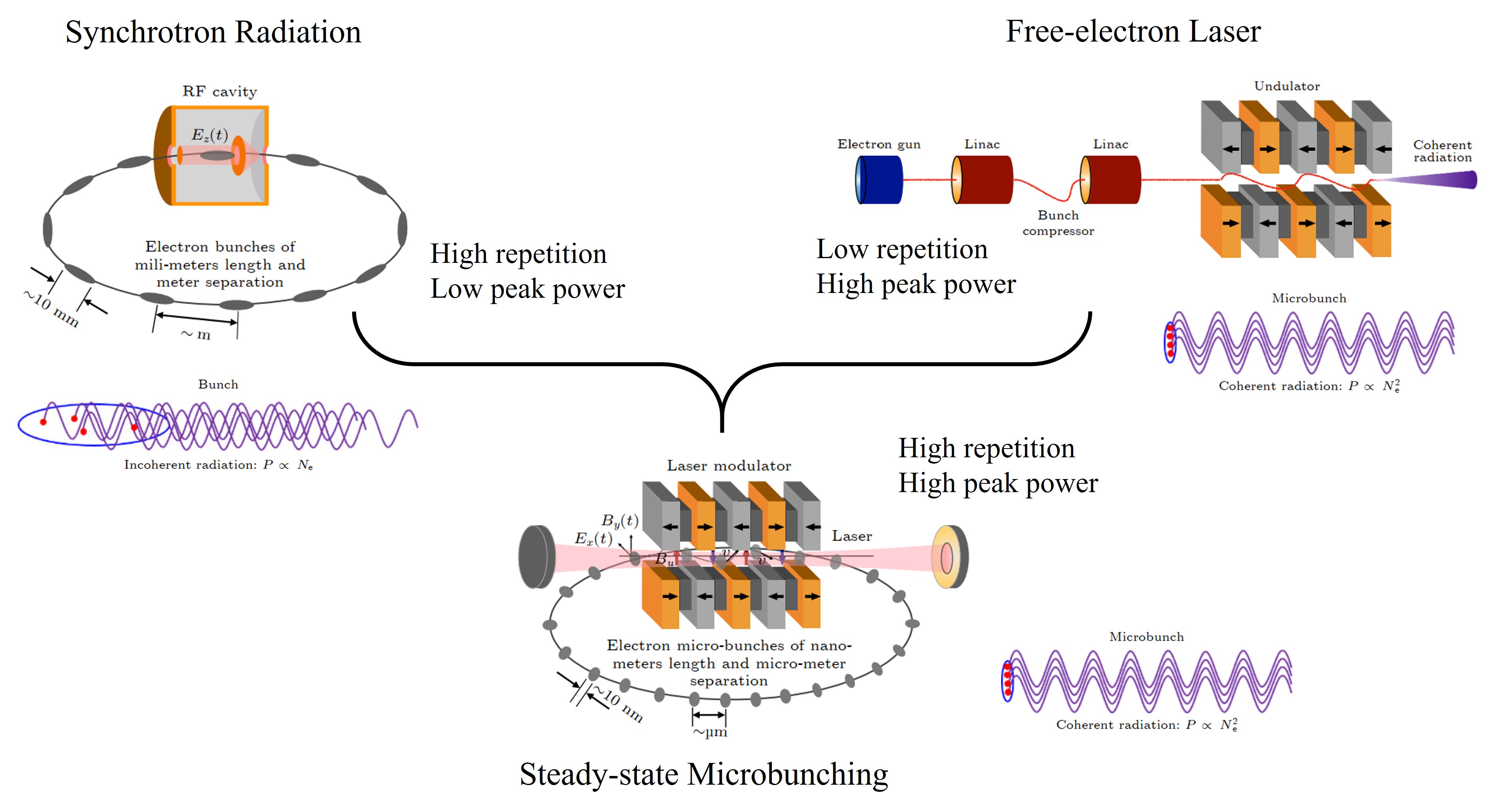
Figure 1: A schematic layout of an SSMB ring, and comparison to synchrotron radiation source and free-electron laser. (Figure adapted from Ref. [4])

The work in this paper is organized as follows. In Sec. 2, we first derive the theoretical minimum longitudinal emittance in an electron storage ring to provide basis for later investigation since SSMB is about realizing short bunch length and small longitudinal emittance. Following this, in Sec. 3, we conduct some key analysis of three specific SSMB scenarios along the thinking of realizing nm bunch length and high-average-power EUV radiation, i.e., longitudinal weak focusing (LWF), longitudinal strong focusing (LSF) and generalized longitudinal strong focusing (GLSF). A short summary of these three schemes is: a LWF SSMB ring can be used to generate bunches with a bunch length of a couple of 10 nm, thus can be used to generate coherent visible and infrared radiation. If we want to push the bunch length to a shorter range, the required phase slippage factor of the LWF ring will be too small from an engineering viewpoint. A LSF SSMB ring can create bunches with a bunch length of nm level, thus to generate coherent EUV radiation. However, the required modulation laser power is in GW level, and makes the laser modulator, which typically consists of an optical enhancement cavity with incident laser and an undulator and is used to imprint energy modulation on or to longitudinally focus the electron beam at the laser wavelength scale, can only work at a low duty cycle pulsed mode, thus limiting the average output EUV radiation power. At present, a GLSF SSMB ring is the most promising among these three to obtain nm bunch length with a mild modulation laser power, thus allowing high-average-power radiation output. The basic idea of GLSF is to exploit the ultrasmall vertical emittance in a planar ring and apply partial transverse-longitudinal emittance for bunch compression with a shallow energy modulation strength, thus small modulation laser power. The backbone of such an GLSF ring is the transverse-longitudinal coupling (TLC) dynamics, which is the focus of this paper. Following this analysis, before going into the concrete examples, we have proven three theorems in Sec. 4 about TLC-based bunch compression or harmonic generation schemes that can be used in our later analysis. After that, we then go into the details of various TLC schemes, with Sec. 5 devoted to energy modulation-based schemes and Sec. 6 dedicated to angular modulation-based schemes. The conclusion from the analysis and comparison is that energy modulation-based coupling is favored for our application in GLSF SSMB. Based on the investigations and other various physical considerations, an engineering practical example parameters set of a 1 kW-average-power EUV light source is finally presented in Sec. 7. A short summary is given in Sec. 8.

2 Theoretical Minimum Emittances

SSMB is about lowering the equilibrium bunch length and longitudinal emittance in an electron storage ring. Before going into the specific SSMB scenarios, it might helpful to derive the theoretical minimum longitudinal emittance in an electron storage ring first. For completeness, here in this section we also present the analysis of theoretical minimum transverse emittance.

Particle state vector ${\bf X}=\left(\begin{matrix}x&x^{\prime}&y&y^{\prime}&z&\delta\end{matrix}\right)^{T}$ is used throughout this paper, with its components meaning horizontal location, angle, vertical location, angle, longitudinal location, and relative energy deviation with respect to the reference particle, respectively. ^T means transpose of a vector or matrix. From Chao’s solution by linear matrix (SLIM) formalism [11], the equilibrium horizontal and longitudinal emittances in a planar uncoupled electron storage ring given by the balance of quantum excitation and radiation damping are

$$\epsilon_{x} \equiv\langle J_{x}\rangle=\frac{55}{96\sqrt{3}}\frac{\alpha_{F}{\lambdabar}_{e}^{2}\gamma^{5}}{\alpha_{H}}\oint\frac{\mathcal{H}_{x}(s)}{|\rho(s)|^{3}}ds,$$ (1)

$$\epsilon_{z} \equiv\langle J_{z}\rangle=\frac{55}{96\sqrt{3}}\frac{\alpha_{F}{\lambdabar}_{e}^{2}\gamma^{5}}{\alpha_{L}}\oint\frac{\beta_{z}(s)}{|\rho(s)|^{3}}ds,$$

in which

$$J_{x} =\frac{\left(x-D_{x}\delta\right)^{2}+\left[\alpha_{x}(x-D_{x}\delta)+\beta_{x}(x^{\prime}-D_{x}^{\prime}\delta)\right]^{2}}{2\beta_{x}},$$ (2)

$$J_{z} =\frac{\left(z+D_{x}^{\prime}x-D_{x}x^{\prime}\right)^{2}+\left[\alpha_{z}(z+D_{x}^{\prime}x-D_{x}x^{\prime})+\beta_{z}\delta\right]^{2}}{2\beta_{z}},$$

are the horizontal and longitudinal action of a particle, and $\langle\rangle$ here means particle ensemble average, $\alpha_{x,z},\beta_{x,z}$ are the Courant-Snyder functions [12] in the horizontal and longitudinal planes, $D_{x}$ and $D_{x}^{\prime}$ are the horizontal dispersion and dispersion angle, and $\mathcal{H}_{x}=\frac{D_{x}^{2}+\left(\alpha_{x}D_{x}+\beta_{x}D_{x}^{\prime}\right)^{2}}{\beta_{x}}$ is the horizontal chromatic function, $\alpha_{F}=\frac{1}{137}$ is the fine-structure constant, $\lambdabar_{e}={\lambda_{e}}/{2\pi}=386\ \text{fm}$ is the reduced Compton wavelength of electron, $\alpha_{H}$ and $\alpha_{L}$ are the horizontal and longitudinal damping constants and in a planar uncoupled ring are given by [13]

$$\alpha_{H}=\frac{U_{0}}{2E_{0}}(1-\mathcal{D}),\ \alpha_{L}=\frac{U_{0}}{2E_{0}}(2+\mathcal{D}),$$ (3)

where $E_{0}$ is the electron energy, $U_{0}$ is the radiation energy loss per particle per turn, $\mathcal{D}=\frac{\oint\frac{(1-2n)D_{x}}{\rho^{3}}ds}{\oint\frac{1}{\rho^{2}}ds}$, with $n=-\frac{\rho}{B_{y}}\frac{\partial B_{y}}{\partial x}$ the field gradient index. Nominally, $|\mathcal{D}|\ll 1$.

2.1 Theoretical Minimum Transverse Emittance

From Eq. (1) we can see that $\mathcal{H}_{x}$ and $\beta_{z}$ at the bending magnets are of vital importance in determining the horizontal and longitudinal emittance. Therefore, we need to know how they evolve inside a bending magnet. The transfer matrix of a sector bending magnet is

$${\bf S}(\alpha)=\left(\begin{array}[]{cccccc}\cos\alpha&\rho\sin\alpha&0&0&0&\rho(1-\cos\alpha)\\ -\frac{\sin\alpha}{\rho}&\cos\alpha&0&0&0&\sin\alpha\\ 0&0&1&\rho\alpha&0&0\\ 0&0&0&1&0&0\\ -\sin\alpha&-\rho(1-\cos\alpha)&0&0&1&\rho\left(\frac{\alpha}{\gamma^{2}}-\alpha+\sin\alpha\right)\\ 0&0&0&0&0&1\\ \end{array}\right),$$ (4)

with $\rho$ and $\alpha$ the bending radius and angle of the bending magnet. In a planar uncoupled ring, the normalized eigenvector corresponding to the horizontal and vertical eigenmode at the dipole middle point is

$${\bf E}_{I}(0)=\frac{1}{\sqrt{2}}\left(\begin{matrix}\sqrt{\beta_{x0}}\\ \frac{i-\alpha_{x0}}{\sqrt{\beta_{x0}}}\\ 0\\ 0\\ -\sqrt{\beta_{x0}}D_{x0}^{\prime}+\frac{i-\alpha_{x0}}{\sqrt{\beta_{x0}}}D_{x0}\\ 0\end{matrix}\right)e^{i\Phi_{I0}},\ {\bf E}_{III}(0)=\frac{1}{\sqrt{2}}\left(\begin{matrix}\frac{i-\alpha_{z0}}{\sqrt{\beta_{z0}}}D_{x0}\\ \frac{i-\alpha_{z0}}{\sqrt{\beta_{z0}}}D_{x0}^{\prime}\\ 0\\ 0\\ \sqrt{\beta_{z0}}\\ \frac{i-\alpha_{z0}}{\sqrt{\beta_{z0}}}\end{matrix}\right)e^{i\Phi_{III0}},$$ (5)

where $\alpha_{x0},\beta_{x0},\alpha_{z0},\beta_{z0},D_{x0},D_{x0}^{\prime}$ are the optical functions at the dipole middle point. From Eqs. (4) and (5) we have the evolution of $\mathcal{H}_{x}$ evolution in the dipole

$$\mathcal{H}_{x}(\alpha) \equiv\beta_{55}^{I}(\alpha)=2|{\bf E}_{I5}(\alpha)|^{2}=2|\left({\bf S}(\alpha){\bf E}_{I}(0)\right)_{5}|^{2}$$ (6)

$$=\left(\sqrt{\beta_{x0}}\left(\sin\alpha+D_{x0}^{\prime}\right)+\frac{\alpha_{x0}}{\sqrt{\beta_{x0}}}\left[D_{x0}-\rho(1-\cos\alpha)\right]\right)^{2}+\left(\frac{D_{x0}-\rho(1-\cos\alpha)}{\sqrt{\beta_{x0}}}\right)^{2}.$$

Similarly, the evolution of $\beta_{z}$ in the dipole is given by

$$\beta_{z}(\alpha) \equiv\beta_{55}^{III}(\alpha)=2|{\bf E}_{III5}(\alpha)|^{2}=2|\left({\bf S}(\alpha){\bf E}_{III}(0)\right)_{5}|^{2}$$ (7)

$$=\left(\sin\alpha\frac{\alpha_{z0}}{\sqrt{\beta_{z0}}}D_{x0}+\rho(1-\cos\alpha)\frac{\alpha_{z0}}{\sqrt{\beta_{z0}}}D_{x0}^{\prime}+\sqrt{\beta_{z0}}-\rho\left(-\alpha+\sin\alpha\right)\frac{\alpha_{z0}}{\sqrt{\beta_{z0}}}\right)^{2}$$

$$\ \ \ \ +\left(-\sin\alpha\frac{1}{\sqrt{\beta_{z0}}}D_{x0}-\rho(1-\cos\alpha)\frac{1}{\sqrt{\beta_{z0}}}D_{x0}^{\prime}+\rho\left(-\alpha+\sin\alpha\right)\frac{1}{\sqrt{\beta_{z0}}}\right)^{2}.$$

Note that $\beta_{55}^{I}$ and $\beta_{55}^{III}$ here are the generalized beta functions defined in Ref. [14]. We have neglected the contribution of $\frac{\rho\alpha}{\gamma^{2}}$ to $R_{56}$ of dipole in the above calculation of $\beta_{z}$, since we are interested in the relativistic cases. But we remind the readers that in a quasi-isochronous ring, the contribution of $\frac{C_{0}}{\gamma^{2}}$ with $C_{0}$ the ring circumference to the ring $R_{56}$ or phase slippage may not be negligible.

With the evolution of $\mathcal{H}_{x}$ and $\beta_{z}$ known, now we derive the theoretical minimum emittances. For simplicity, we assume the ring consists of iso-bending-magnets, and the optical functions are identical in each bending magnets. Further, here we assume the damping partition $\mathcal{D}$ is close to zero. With these assumptions and simplification, putting $\alpha_{H}\approx\frac{U_{0}}{2E_{0}}=\frac{1}{2}C_{\gamma}\frac{E_{0}^{3}}{\rho}$ in Eq. (1), we have

$$\epsilon_{x} =\frac{55\pi}{24\sqrt{3}}\frac{\alpha_{F}\lambdabar_{e}^{2}\gamma^{5}}{C_{\gamma}E_{0}^{3}}\frac{1}{\rho}f_{x}(\alpha_{x0},\beta_{x0},D_{x0},D_{x0}^{\prime}),$$ (8)

with

$$f_{x}(\alpha_{x0},\beta_{x0},D_{x0},D_{x0}^{\prime})=\frac{1}{\theta}\int_{-\frac{\theta}{2}}^{\frac{\theta}{2}}\mathcal{H}_{x}(\alpha)d\alpha,$$ (9)

which can be interpreted as the average $\mathcal{H}_{x}$ in the dipole. The lengthy expression of $f_{x}(\alpha_{x0},\beta_{x0},D_{x0},D_{x0}^{\prime})$ is omitted here. It can be obtained straightforwardly for example using Mathematica, by inserting Eq. (6) in Eq. (9). The mathematical problem we are trying to solve is then to minimize $f_{x}$, by adjusting $\alpha_{x0}$, $\beta_{x0}$, $D_{x0}$, $D_{x0}^{\prime}$. From Eq. (9) we have

$$\frac{\partial f_{x}}{\partial\alpha_{x0}} =\alpha_{x0}\frac{2D_{x0}\left(D_{x0}-2\rho+2\rho\frac{\sin\frac{\theta}{2}}{\frac{\theta}{2}}\right)+\rho^{2}\left(3-4\frac{\sin\frac{\theta}{2}}{\frac{\theta}{2}}+\frac{\sin\theta}{\theta}\right)}{\beta_{x0}}+D_{x0}^{\prime}2\left(D_{x0}-\rho+\rho\frac{\sin\frac{\theta}{2}}{\frac{\theta}{2}}\right),$$ (10)

$$\frac{\partial f_{x}}{\partial D_{x0}^{\prime}} =\alpha_{x0}2\left(D_{x0}-\rho+\rho\frac{\sin\frac{\theta}{2}}{\frac{\theta}{2}}\right)+D_{x0}^{\prime}2\beta_{x0}.$$

We notice that the requirement of $\frac{\partial f_{x}}{\partial\alpha_{x0}}=0$ and $\frac{\partial f_{x}}{\partial D_{x0}^{\prime}}=0$ leads to $\alpha_{x0}=0$ and $D_{x0}^{\prime}=0$. Under the above conditions, then

$$\frac{\partial f_{x}}{\partial D_{x0}} =\frac{2\left(D_{x0}-\rho+\rho\frac{\sin\frac{\theta}{2}}{\frac{\theta}{2}}\right)}{\beta_{x0}}.$$ (11)

The requirement of $\frac{\partial f_{x}}{\partial D_{x0}}=0$ leads to

$$D_{x0} =\rho\left(1-\frac{\sin\frac{\theta}{2}}{\frac{\theta}{2}}\right)\approx\frac{\rho\theta^{2}}{24}.$$ (12)

Under the above conditions, then

$$\frac{\partial f_{x}}{\partial\beta_{x0}} =\frac{\theta(\theta-\sin\theta)-\frac{\rho^{2}\left(\theta^{2}+\theta\sin\theta+4\cos\theta-4\right)}{\beta_{x0}^{2}}}{2\theta^{2}}.$$ (13)

The requirement of $\frac{\partial f_{x}}{\partial\beta_{x0}}=0$ leads to

$$\beta_{x0} =\rho\sqrt{\frac{\left(\theta^{2}+\theta\sin\theta+4\cos\theta-4\right)}{\theta(\theta-\sin\theta)}}\approx\frac{\rho\theta}{2\sqrt{15}}.$$ (14)

Summarizing, the extreme value of $f_{x}$ and thus the horizontal emittance $\epsilon_{x}$ is realized when

$$\alpha_{x0} =0,\ \beta_{x0}\approx\frac{\rho\theta}{2\sqrt{15}},\ D_{x0}\approx\frac{\rho\theta^{2}}{24},\ D_{x0}^{\prime}=0,\$$ (15)

which means

$$\mathcal{H}_{x0}=\frac{D_{x0}^{2}}{\beta_{x0}}=\rho\frac{\left(1-\frac{\sin\frac{\theta}{2}}{\frac{\theta}{2}}\right)^{2}}{\sqrt{\frac{\left(\theta^{2}+\theta\sin\theta+4\cos\theta-4\right)}{\theta(\theta-\sin\theta)}}}\approx\frac{5\rho\theta^{3}}{96\sqrt{15}},$$ (16)

and

$$f_{x,\text{min}} =\rho\left(1-\frac{\sin\theta}{\theta}\right)\sqrt{\frac{\left(\theta^{2}+\theta\sin\theta+4\cos\theta-4\right)}{\theta(\theta-\sin\theta)}}\approx\frac{\rho\theta^{3}}{12\sqrt{15}}.$$ (17)

The above results are consistent with the classical results of Teng [15]. Note that $f_{x,\text{min}}=\frac{8}{5}\mathcal{H}_{x0}$. One can check that this extreme emittance is the minimum emittance. For practical use, let us put in the numbers, we then have the theoretical minimum horizontal emittance scaling

$$\epsilon_{x,\text{min}}[\text{nm}]=31.5E^{2}_{0}[\text{GeV}]\theta^{3}[\text{rad}].$$ (18)

For example, if $E_{0}=6$ GeV and $\theta=\frac{2\pi}{300}$ rad, we have $\epsilon_{x,\text{min}}=10.4$ pm.

2.2 Theoretical Minimum Longitudinal Emittance

Now we analyze the theoretical minimum longitudinal emittance. Putting $\alpha_{L}\approx\frac{U_{0}}{E_{0}}=C_{\gamma}\frac{E_{0}^{3}}{\rho}$ in Eq. (1), we have

$$\epsilon_{z} =\frac{55\pi}{48\sqrt{3}}\frac{\alpha_{F}\lambdabar_{e}^{2}\gamma^{5}}{C_{\gamma}E_{0}^{3}}\frac{1}{\rho}f_{z}(\alpha_{z0},\beta_{z0},D_{x0},D_{x0}^{\prime}),$$ (19)

with

$$f_{z}(\alpha_{z0},\beta_{x0},D_{x0},D_{x0}^{\prime})=\frac{1}{\theta}\int_{-\frac{\theta}{2}}^{\frac{\theta}{2}}\beta_{z}(\alpha)d\alpha,$$ (20)

which can be interpreted as the average $\beta_{z}$ in the dipole. Then

$$\frac{\partial f_{z}}{\partial\alpha_{z0}} =\alpha_{{z0}}t(\rho,\theta,D_{x0},D_{x0}^{\prime},\beta_{z0})+D_{x0}^{\prime}2\rho\left(1-\frac{\sin\frac{\theta}{2}}{\frac{\theta}{2}}\right),$$ (21)

$$\frac{\partial f_{z}}{\partial D_{x0}^{\prime}} =\alpha_{{z0}}2\rho\left(1-\frac{\sin\frac{\theta}{2}}{\frac{\theta}{2}}\right)+D_{x0}^{\prime}\frac{\left(1+\alpha_{{z0}}^{2}\right)\rho^{2}\left(3-4\frac{\sin\frac{\theta}{2}}{\frac{\theta}{2}}+\frac{\sin\theta}{\theta}\right)}{\beta_{z0}},$$

where the lengthy expression of $t(\rho,\theta,D_{x0},D_{x0}^{\prime},\beta_{z0})$ is omitted here. Similar to the analysis of transverse minimum emittance, we notice again that the requirement of $\frac{\partial f_{z}}{\partial\alpha_{z0}}=0$ and $\frac{\partial f_{z}}{\partial D_{x0}^{\prime}}=0$ leads to $\alpha_{z0}=0$ and $D_{x0}^{\prime}=0$. Under the above conditions, then

$$\frac{\partial f_{z}}{\partial D_{x0}} =\frac{D_{x0}\left(1-\frac{\sin\theta}{\theta}\right)-\rho\left(1-\frac{\sin\theta}{\theta}-2\frac{\sin\frac{\theta}{2}}{\frac{\theta}{2}}+2\cos\frac{\theta}{2}\right)}{\beta_{z0}}.$$ (22)

The requirement of $\frac{\partial f_{z}}{\partial D_{x0}}=0$ leads to

$$D_{x0} =\frac{\rho\left(1-\frac{\sin\theta}{\theta}-2\frac{\sin\frac{\theta}{2}}{\frac{\theta}{2}}+2\cos\frac{\theta}{2}\right)}{1-\frac{\sin\theta}{\theta}}\approx-\frac{\rho\theta^{2}}{40}.$$ (23)

Under the above conditions, then

$$\frac{\partial f_{z}}{\partial\beta_{z0}} =1-\frac{\rho^{2}\left(\theta^{4}-12\theta^{2}-\left(\theta^{2}-48\right)\theta\sin\theta-12\left(\theta^{2}-4\right)\cos\theta-48\right)}{12\theta(\theta-\sin\theta)\beta_{z0}^{2}}.$$ (24)

The requirement of $\frac{\partial f_{z}}{\partial\beta_{z0}}=0$ leads to

$$\beta_{z0} =\rho\sqrt{\frac{\left(\theta^{4}-12\theta^{2}-\left(\theta^{2}-48\right)\theta\sin\theta-12\left(\theta^{2}-4\right)\cos\theta-48\right)}{12\theta(\theta-\sin\theta)}}\approx\frac{\rho\theta^{3}}{120\sqrt{7}},$$ (25)

Summarizing, the extreme value of $f_{z}$ and the longitudinal emittance is realized when

$$\alpha_{z0} =0,\ \beta_{z0}\approx\frac{\rho\theta^{3}}{120\sqrt{7}},\ D_{x0}\approx-\frac{\rho\theta^{2}}{40},\ D_{x0}^{\prime}=0,$$ (26)

and

$$f_{z,\text{min}} =\rho\sqrt{\frac{\left(\theta^{4}-12\theta^{2}-\left(\theta^{2}-48\right)\theta\sin\theta-12\left(\theta^{2}-4\right)\cos\theta-48\right)}{3\theta(\theta-\sin\theta)}}\approx\frac{\rho\theta^{3}}{60\sqrt{7}}.$$ (27)

The above result has also been given in Ref. [16]. Note that $f_{z,\text{min}}=2\beta_{z0}$. One can check that this extreme emittance is the minimum emittance. For practical use, let us put in the numbers, we then have the theoretical minimum longitudinal emittance scaling

$$\epsilon_{z,\text{min}}[\text{nm}]=4.61E^{2}_{0}[\text{GeV}]\theta^{3}[\text{rad}].$$ (28)

For example, if $E_{0}=0.6$ GeV and $\theta=\frac{2\pi}{50}$ rad, we have $\epsilon_{z,\text{min}}=3.3$ pm.

Here we remind the readers that in reality it may not easy to reach the optimal conditions Eq. (26) for all the dipoles in a ring, since it may not easy to apply too many RFs or laser modulators in a ring to manipulate the longitudinal optics, while in transverse dimension it is straightforward to implement many quadrupoles to manipulate the transverse optics. Instead, we may choose a more practical strategy to realize small longitudinal emittance, which is letting each half of the bending magnet isochronous, and the longitudinal optics for each dipole can then be identical. Under such condition, the minimum longitudinal emittance is [8]

$$\epsilon_{z,\text{min},\text{ISO}}[\text{nm}]=8.44E^{2}_{0}[\text{GeV}]\theta^{3}[\text{rad}],$$ (29)

and is realized when

$$\alpha_{z0} =0,\ \beta_{z0}\approx\frac{\sqrt{210}}{2520}\rho\theta^{3},\ D_{x0}\approx-\frac{\rho\theta^{2}}{24},\ D_{x0}^{\prime}=0.$$ (30)

In this case, we still have $f_{z}=2\beta_{z0}$. The emittance given in Eq. (29) is larger than the theoretical minimum Eq. (28). Based on this emittance and $\beta_{z0}$, we can know the bunch length in the dipole center contributed from longitudinal emittance. We remind the readers that the bunch length can in principle be even smaller than this value, by pushing $\beta_{z0}$ to an even smaller value, although the longitudinal emittance will actually grow then. However, if the ring works in a longitudinal weak focusing regime to be introduced in next section, there is a lower limit of bunch length in this process, which is a factor of $\sqrt{2}$ smaller than the bunch length given by conditions of Eqs. (29) and (30). Putting in the numbers, we have this lower limit of bunch length in a longitudinal weak focusing ring

$$\sigma_{z,\text{min},\text{ISO}}[\mu\text{m}]=4.93\rho^{\frac{1}{2}}[\text{m}]E_{0}[\text{GeV}]\theta^{3}[\text{rad}].$$ (31)

For example, if $E_{0}=0.6$ GeV, $\rho=1.5$ m ($B_{0}=1.33$ T) and $\theta=\frac{2\pi}{50}$ rad, then $\sigma_{z,\text{min},\text{ISO}}=7.2$ nm. The energy spread will diverge when we push the bunch length to this limit [17].

2.3 Application of Transverse Gradient Bend

The previous analysis assumes that the transverse gradient of bending field is zero. Now we consider the application of transverse gradient bending (TGB) magnets to lower horizontal and longitudinal emittances. For simplicity, we will consider the case of a constant gradient. The transfer matrix of a sector bending magnet with a constant transverse gradient $n=-\frac{\rho}{B_{y}}\frac{\partial B_{y}}{\partial x}$ is

$$\begin{split}{\bf S}_{\text{TGB}}(\alpha)=&\left(\begin{array}[]{cccccc}\cos\left(\sqrt{1-n}\alpha\right)&\frac{\rho}{\sqrt{1-n}}\sin\left(\sqrt{1-n}\alpha\right)&0\\ -\frac{\sqrt{1-n}}{\rho}\sin\left(\sqrt{1-n}\alpha\right)&\cos\left(\sqrt{1-n}\alpha\right)&0\\ 0&0&\cos\left(\sqrt{n}\alpha\right)\\ 0&0&-\frac{\sqrt{n}}{\rho}\sin\left(\sqrt{n}\alpha\right)\\ -\frac{1}{\sqrt{1-n}}\sin\left(\sqrt{1-n}\alpha\right)&-\frac{\rho}{1-n}\left(1-\cos\left(\sqrt{1-n}\alpha\right)\right)&0\\ 0&0&0\\ \end{array}\right.\\ &\ \ \ \ \ \ \ \ \ \left.\begin{array}[]{cccccc}0&0&\frac{\rho}{1-n}\left(1-\cos\left(\sqrt{1-n}\alpha\right)\right)\\ 0&0&\frac{1}{\sqrt{1-n}}\sin\left(\sqrt{1-n}\alpha\right)\\ \frac{\rho}{\sqrt{n}}\sin\left(\sqrt{n}\alpha\right)&0&0\\ \cos\left(\sqrt{n}\alpha\right)&0&0\\ 0&1&\frac{\rho\alpha}{\gamma^{2}}+\frac{\rho}{\left(1-n\right)^{\frac{3}{2}}}\left(-\sqrt{1-n}\alpha+\sin\left(\sqrt{1-n}\alpha\right)\right)\\ 0&0&1\\ \end{array}\right).\end{split}$$ (32)

2.3.1 Horizontal Emittance

Similar to steps presented in the previous analysis, we find the minimum value of $f_{x}$ in Eq. (9) is now realized when

$$\alpha_{x0} =0,\ \beta_{x0}\approx\frac{\rho\theta}{2\sqrt{15}}\left[1+\frac{(1-n)\theta^{2}}{140}\right]+\mathcal{O}(\theta^{6}),$$ (33)

$$D_{x0} \approx\frac{\rho\theta^{2}}{24}\left[1-\frac{(1-n)\theta^{2}}{48}\right]+\mathcal{O}(\theta^{6}),\ D_{x0}^{\prime}=0,\$$

which means

$$\mathcal{H}_{x0}=\frac{D_{x0}^{2}}{\beta_{x0}}\approx\frac{5\rho\theta^{3}}{96\sqrt{15}}\left[1-\frac{9(1-n)\theta^{2}}{280}\right]+\mathcal{O}(\theta^{7}),$$ (34)

and

$$f_{x,\text{min}} \approx\frac{\rho\theta^{3}}{12\sqrt{15}}\left[1-\frac{3(1-n)\theta^{2}}{70}\right]+\mathcal{O}(\theta^{7}).$$ (35)

So we have

$$\epsilon_{x,\text{min}}[\text{nm}]=31.5E^{2}_{0}[\text{GeV}]\theta^{3}[\text{rad}]\left[1-\frac{3(1-n)\theta^{2}}{70}\right].$$ (36)

Therefore, the impact of transverse gradient on the theoretical minimum emittance is on the higher order of the bending angle. However, we should note that $n$ can be a quite large value in practice. So its impact may actually not small. In addition, a transverse gradient bend can also affect the damping partition, whose details we do not go into here.

2.3.2 Longitudinal Emittance

Similarly, using TGB, the minimum value of $f_{z}$ in Eq. (20) is realized when

$$\alpha_{z0} =0,\ \beta_{z0}\approx\frac{\rho\theta^{3}}{120\sqrt{7}}\left[1+\frac{(1-n)\theta^{2}}{90}\right]+\mathcal{O}(\theta^{7}),$$ (37)

$$D_{x0} \approx-\frac{\rho\theta^{2}}{40}\left[1+\frac{19(1-n)\theta^{2}}{1680}\right]+\mathcal{O}(\theta^{6}),\ D_{x0}^{\prime}=0,\$$

and

$$f_{z,\text{min}} \approx\frac{\rho\theta^{3}}{60\sqrt{7}}\left[1+\frac{(1-n)\theta^{2}}{90}\right]+\mathcal{O}(\theta^{7}).$$ (38)

Note that $f_{z,\text{min}}=2\beta_{z0}$ still holds here. So we have

$$\epsilon_{z,\text{min}}[\text{nm}]=4.61E^{2}_{0}[\text{GeV}]\theta^{3}[\text{rad}]\left[1+\frac{(1-n)\theta^{2}}{90}\right].$$ (39)

2.4 Application of Longitudinal Gradient Bend

We can also apply longitudinal gradient bend (LGB) to lower the transverse and longitudinal emittance. For simplicity, we will study the case of a LGB consisting of several sub-dipoles with each a constant bending radius. Further, we will assume each sub-dipole is a sector dipole. The analysis for the case of rectangular dipoles is similar, as long as the impact of edge angles on transfer matrix and damping partition have been properly handled. Now we investigate the case of sector sub-dipoles. For example, we may choose to let the LGB has a symmetric structure

$$(\rho_{2},\theta_{2}),(\rho_{1},\theta_{1}),(\rho_{0},2\theta_{0}),(\rho_{1},\theta_{1}),(\rho_{2},\theta_{2})$$ (40)

The total bending angle of such a LGB is $\theta_{T}=2(\theta_{0}+\theta_{1}+\theta_{2})$, and the total length is $2(\rho_{0}\theta_{0}+\rho_{1}\theta_{1}+\rho_{2}\theta_{2})$. Note that $\rho_{i}\theta_{i}\geq 0$. We use this structure as an example for the analysis. The presented method however applies to more general setup.

2.4.1 Horizontal Emittance

Now we calculate the theoretical minimum horizontal emittance by invoking LGBs with each the structure given in Eq. (40). The damping constant of the horizontal mode is

$$\alpha_{H}\approx\frac{U_{0}}{2E_{0}}=\frac{1}{2}C_{\gamma}E_{0}^{3}\left[\frac{\theta_{0}}{\rho_{0}(\theta_{0}+\theta_{1}+\theta_{2})}+\frac{\theta_{1}}{\rho_{1}(\theta_{0}+\theta_{1}+\theta_{2})}+\frac{\theta_{2}}{\rho_{2}(\theta_{0}+\theta_{1}+\theta_{2})}\right].$$ (41)

Still we assume all the LGBs and optical functions in them are identical, then

$$\epsilon_{x} =\frac{55}{96\sqrt{3}}\frac{\alpha_{F}\lambdabar_{e}^{2}\gamma^{5}}{\alpha_{H}}\oint\frac{\mathcal{H}_{x}}{|\rho|^{3}}ds$$ (42)

$$=\frac{55\pi}{24\sqrt{3}}\frac{\alpha_{F}\lambdabar_{e}^{2}\gamma^{5}}{C_{\gamma}E_{0}^{3}}F_{x}(\alpha_{x0},\beta_{x0},D_{x0},D_{x0}^{\prime}),$$

with

$$F_{x}(\alpha_{x0},\beta_{x0},D_{x0},D_{x0}^{\prime})=\frac{1}{2\left(\frac{\theta_{0}}{\rho_{0}}+\frac{\theta_{1}}{\rho_{1}}+\frac{\theta_{2}}{\rho_{2}}\right)}\int_{-(\rho_{0}\theta_{0}+\rho_{1}\theta_{1}+\rho_{2}\theta_{2})}^{(\rho_{0}\theta_{0}+\rho_{1}\theta_{1}+\rho_{2}\theta_{2})}\frac{\mathcal{H}_{x}(s)}{|\rho(s)|^{3}}ds.$$ (43)

Note that the dimension of $F_{x}$ here is equivalent to $\frac{f_{x}}{\rho}$ given in previous sections. The mathematical problem is then to minimize $F_{x}(\alpha_{x0},\beta_{x0},D_{x0},D_{x0}^{\prime})$, by adjusting $\alpha_{x0}$, $\beta_{x0}$, $D_{x0}$, $D_{x0}^{\prime}$. The calculation method of $\mathcal{H}_{x}$ evolution in LGB is the same as that given in Eq. (6), but note that here for different part (sub-dipole) of the LGBs, we should apply the transfer matrix from the middle point of LGB to the corresponding location. Following similar procedures, we find that to get the minimum emittance, we need $\alpha_{x0}=0$ and $D_{x0}^{\prime}=0$. Then we have $\mathcal{H}_{x}(-s)=\mathcal{H}_{x}(s)$, which means

$$F_{x}=\frac{1}{\left(\frac{\theta_{0}}{\rho_{0}}+\frac{\theta_{1}}{\rho_{1}}+\frac{\theta_{2}}{\rho_{2}}\right)}\left(\int_{0}^{\rho_{0}\theta_{0}}\frac{\mathcal{H}_{x}(s)}{|\rho_{0}|^{3}}ds+\int_{\rho_{0}\theta_{0}}^{\rho_{0}\theta_{0}+\rho_{1}\theta_{1}}\frac{\mathcal{H}_{x}(s)}{|\rho_{1}|^{3}}ds+\int_{\rho_{0}\theta_{0}+\rho_{1}\theta_{1}}^{\rho_{0}\theta_{0}+\rho_{1}\theta_{1}+\rho_{2}\theta_{2}}\frac{\mathcal{H}_{x}(s)}{|\rho_{2}|^{3}}ds\right).$$ (44)

We find a general analytical discussion of the combination of $\rho_{i}$ and $\theta_{i}$ complicated. Here for simplicity and to get a concrete feeling, we first consider one specific case: $\rho_{i}=\rho_{0}2^{i}$. The physical consideration behind this choice is that $\mathcal{H}_{x}$ will be smaller in the central part of the bending magnet, and larger at the entrance and exit. So we make the bending field in the center stronger and smaller at the entrance and exit. For example, we may choose

$$\left(4\rho,\frac{\theta}{8}\right),\left(2\rho,\frac{\theta}{8}\right),\left(\rho,\frac{\theta}{4}\right),\left(\rho,\frac{\theta}{4}\right),\left(2\rho,\frac{\theta}{8}\right),\left(4\rho,\frac{\theta}{8}\right).$$ (45)

The total length of sush a LGB is $2\rho\theta$. The minimum value of $F_{x}$ and horizontal emittance $\epsilon_{x}$ in this case is realized when

$$\alpha_{x0} =0,\ \beta_{x0}\approx\frac{\sqrt{\frac{35977}{133755}}\rho\theta}{4},\ D_{x0}\approx\frac{127\rho\theta^{2}}{7104},\ D_{x0}^{\prime}=0,\$$ (46)

which means

$$\mathcal{H}_{x0}=\frac{D_{x0}^{2}}{\beta_{x0}}\approx 0.183\times\frac{5}{96\sqrt{15}}\rho\theta^{3},$$ (47)

and

$$F_{x,\text{min}} \approx 0.344\times\frac{f_{x,\text{min}}}{\rho},$$ (48)

which means the theoretical minimum horizontal emittance can now become about a factor of three smaller than the case of no longitudinal gradient. So application of LGB is quite effective in lowering the transverse emittance.

The next question is: what is the optimal combination ratio of $\theta_{0,1,2}$ and $\rho_{0,1,2}$? This questions is not straightforward to answer by analytical method. Here we refer to numerical method to do the optimization directly. $\alpha_{x0}$ and $D_{x0}^{\prime}$ are set to be zero in the optimization. The variables in the numerical optimization are $(\theta_{0},\theta_{1},\theta_{2},\rho_{0},\rho_{1},\rho_{2},\beta_{x0},D_{x0})$. Two optimization goals are $\frac{\epsilon_{x,\text{LGB}}}{\epsilon_{x,\text{UB}}}$ and $L_{\text{LGB}}$, where $\epsilon_{x,\text{UB}}$ is the theoretical minimum emittance of applying bending magnet without longitudinal gradient. We require $\rho_{i}\theta_{i}>0$. In the optimization, we keep the total bending angle a constant value. So the mathematical problem is to minimize $\frac{\epsilon_{x,\text{LGB}}}{\epsilon_{x,\text{UB}}}=\frac{F_{x}}{\frac{f_{x,\text{min}}}{\rho}}=\frac{3\sqrt{15}F_{x}}{2\left(\theta_{0}+\theta_{1}+\theta_{2}\right)^{3}}$ with each given $L_{\text{LGB}}$. The optimization result of one specific case where $\theta_{T}=2(\theta_{0}+\theta_{1}+\theta_{2})=\frac{\pi}{10}$ is presented in Fig. 2, from which we can see that in this case by applying LGBs, in principle we can lower the horizontal emittance by a factor of five with a reasonable total length of the LGB. Note that in this optimization and the one in the following section, we have assumed that $\rho_{i}>0$, so the case of applying anti-bend is not considered.

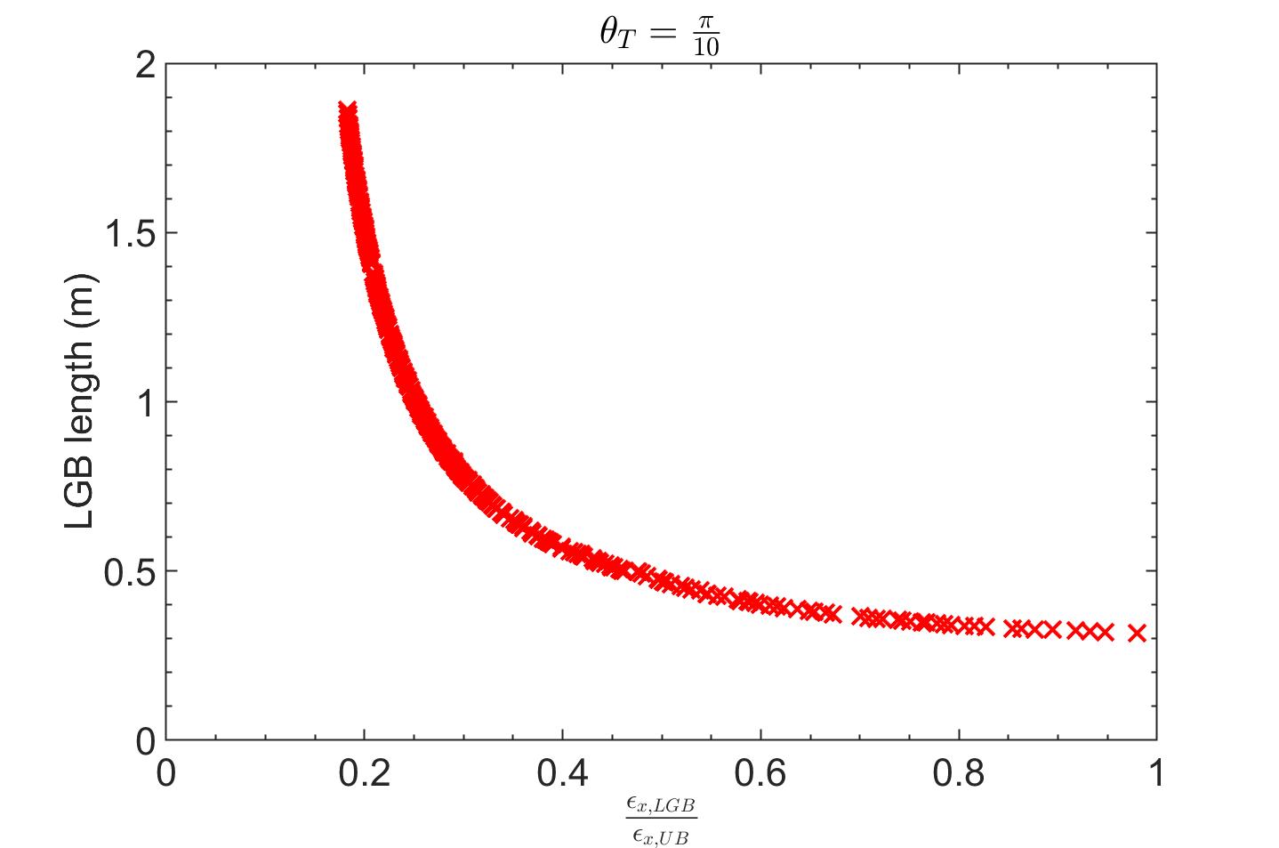
Figure 2: Application of LGB to minimize horizontal emittance. The subscripts ”LGB” and ”UB” represent longitudinal gradient bend and uniform bend, respectively.

2.4.2 Longitudinal Emittance

Similarly, for longitudinal emittance we have

$$\epsilon_{z} =\frac{55\pi}{48\sqrt{3}}\frac{\alpha_{F}\lambdabar_{e}^{2}\gamma^{5}}{C_{\gamma}E_{0}^{3}}F_{z}(\alpha_{z0},\beta_{z0},D_{x0},D_{x0}^{\prime})$$ (49)

with

$$F_{z}(\alpha_{z0},\beta_{z0},D_{x0},D_{x0}^{\prime})=\frac{1}{2\left(\frac{\theta_{0}}{\rho_{0}}+\frac{\theta_{1}}{\rho_{1}}+\frac{\theta_{2}}{\rho_{2}}\right)}\oint_{-(\rho_{0}\theta_{0}+\rho_{1}\theta_{1}+\rho_{2}\theta_{2})}^{(\rho_{0}\theta_{0}+\rho_{1}\theta_{1}+\rho_{2}\theta_{2})}\frac{\beta_{z}(s)}{|\rho(s)|^{3}}ds.$$ (50)

For example, if we choose

$$\left(4\rho,\frac{\theta}{8}\right),\left(2\rho,\frac{\theta}{8}\right),\left(\rho,\frac{\theta}{4}\right),\left(\rho,\frac{\theta}{4}\right),\left(2\rho,\frac{\theta}{8}\right),\left(4\rho,\frac{\theta}{8}\right).$$ (51)

The total length of sush a LGB is $2\rho\theta$. The minimum value of $F_{z}$ and longitudinal emittance in this case is realized when

$$\alpha_{z0} =0,\ \beta_{z0}\approx\frac{\sqrt{\frac{36233641}{62419}}\rho\theta^{3}}{7680},\ D_{x0}\approx-\frac{169\rho\theta^{2}}{9640},\ D_{x0}^{\prime}=0,\$$ (52)

and

$$F_{z,\text{min}} \approx 0.838\times\frac{f_{z,\text{min}}}{\rho},$$ (53)

which means the theoretical minimum longitudinal emittance now can become a bit smaller than the case of applying a constant bending field.

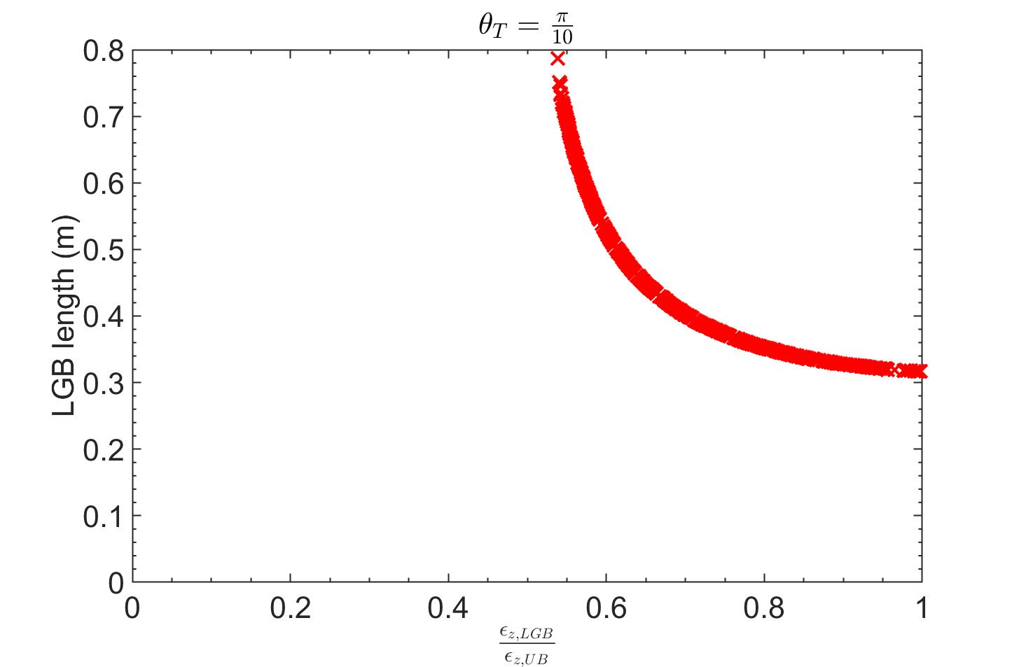
Figure 3: Application of LGB to minimize longitudinal emittance. The subscripts ”LGB” and ”UB” represent longitudinal gradient bend and uniform bend, respectively.

Similar to what presented just now about lowering transverse emittance, we also apply the numerical optimization to choose a better combination of $\rho_{i}$ and $\theta_{i}$ in lowering longitudinal emittance. Presented in Fig. 3 is the result of one specific case where $\theta_{T}=2(\theta_{0}+\theta_{1}+\theta_{2})=\frac{\pi}{10}$, from which we can see that in this case by applying LGBs, in principle we can lower the longitudinal emittance by a factor of two with a reasonable total length of the LGB. So generally, LGB is more effective in lowering the horizontal emittance, compared to lowering the longitudinal emittance.

3 Steady-State Micro-Bunching Storage Rings

In this section, based on the theoretical minimum emittance derived in last section, we conduct some key analysis of three specific SSMB scenarios along the thinking of realizing nm bunch length and high-average-power EUV radiation, i.e., longitudinal weak focusing (LWF), longitudinal strong focusing (LSF) and generalized longitudinal strong focusing (GLSF). Hopefully we can convince the readers why GLSF SSMB is our present choice in realizing high-average-power EUV radiation. Before going into the details, here first we use a table (Tab. 1) and a figure (Fig. 4) to briefly summarize the characteristics of these three scenarios. Note that in Fig. 4, the beam distribution in longitudinal phase space are all of the microbunch, whose length is at the laser wavelength range.

Table 1: Main characteristics of LWF, LSF and GLSF SSMB storage rings.

LWF	$\nu_{s}\ll 1$	$\frac{\beta_{z,\text{max}}}{\beta_{z,\text{min}}}\approx 1$	2D phase space dynamics
LSF	$\nu_{s}\sim 1$	$\frac{\beta_{z,\text{max}}}{\beta_{z,\text{min}}}\gg 1$	2D phase space dynamics
GLSF	-	$\frac{\sigma_{z,\text{max}}}{\sigma_{z,\text{min}}}\gg 1$	4D or 6D phase space dynamics

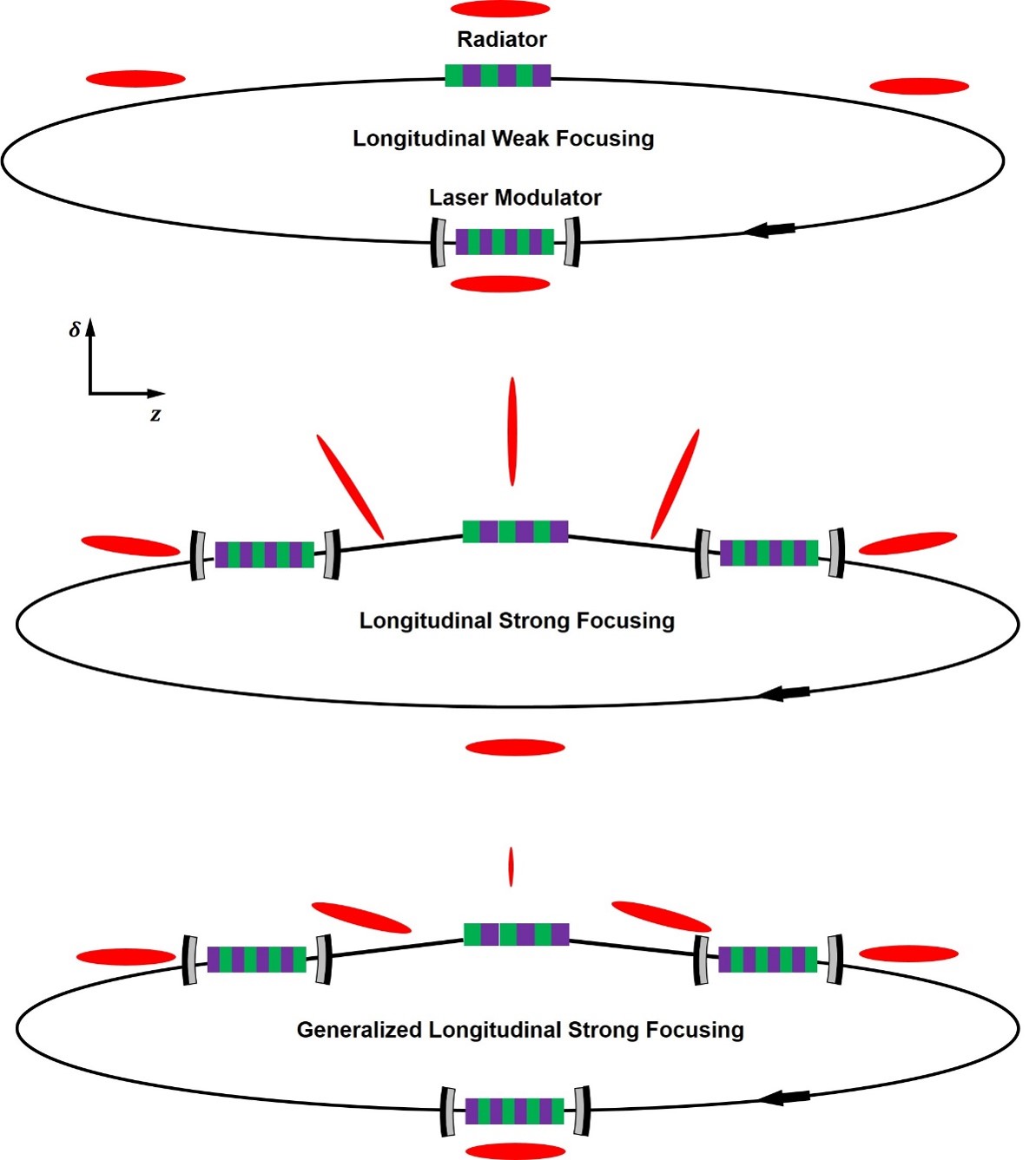
Figure 4: Schematic layout of longitudinal weak focusing, longitudinal strong focusing, generalized longitudinal strong focusing SSMB storage rings. The red ellipses illustrate the beam distribution in longitudinal phase space.

3.1 Longitudinal Weak Focusing

Now we start the quantitative analysis. In all the example calculations to be shown in the following part of this paper, we set the electron energy to be $E_{0}=600$ MeV, and modulation laser wavelength to be $\lambda_{L}=1064$ nm. The choice of this beam energy is because it is an appropriate energy for EUV generation using an undulator as radiator. On one hand, it is not too high, otherwise the laser modulation will become harder. On the other hand, it is not too low otherwise intra-beam scattering (IBS) could become an important issue. The reason for choosing this laser wavelength is due to the fact that it is the common wavelength range choice for high-power optical enhancement cavity, which is used together with an undulator to form the laser modulator of SSMB.

In a longitudinal weak focusing (LWF) ring with a single radiofrequency (RF) cavity or laser modulator as shown in Fig. 4, the single-particle longitudinal dynamics is modeled as

$$\delta =\delta+\frac{h}{k_{L}}\sin(k_{L}z),$$ (54)

$$z =z-\eta C_{0}\delta,$$

where $h$ is the energy chirp strength around the zero-crossing phase, $\eta=\frac{\Delta T/T_{0}}{\Delta E/E_{0}}$ is the phase slippage of the ring, and $C_{0}$ the ring circumference. Note that in the above model, we have assumed that the radiation energy loss in SSMB will be compensated by other system instead of the laser modulators, so the microbunching will be formed around the laser zero-crossing phase. Linear stability requires that $0<h\eta C_{0}<4$. To avoid strong chaotic dynamics which may destroy the regular phase space structure, an empirical criterion is

$$0<h\eta C_{0}\lesssim 0.1.$$ (55)

In a LWF ring, when $|\nu_{s}|\approx\frac{\sqrt{h\eta C_{0}}}{2\pi}\ll 1$, the longitudinal beta function at the middle of RF or laser modulator is [8]

$$\beta_{z\text{M}}\approx\sqrt{\frac{\eta C_{0}}{h}}.$$ (56)

Note that in this paper, we will use subscript ’M’ to represent modulator, and ’R’ to represent radiator. From Eq. (55) we then require

$$\beta_{z\text{M}}\gtrsim\frac{1}{\sqrt{0.1}}|\eta C_{0}|.$$ (57)

Now we can use Eq. (31) and the above result to do some evaluation for a LWF ring. If $E_{0}=600$ MeV, $\rho_{\text{ring}}=1.5$ m ($B_{\text{ring}}=1.33$ T), and if our desired bunch length is $\sigma_{z}=50$ nm ($\sigma_{z}\lesssim\frac{\lambda_{L}}{20}$ to be safely stored in optical microbucket for $\lambda_{L}=1064\$nm), then we may need $\sigma_{z,\text{min},\text{ISO}}\leq\frac{50}{\sqrt{2}}$ nm to avoid significant energy widening when we reach the desired bunch length. From Eq. (31) we then need $\theta\leq 0.2137\ \text{rad}\approx\frac{2\pi}{30}$ rad. Therefore, we need at least 30 bending magnets in the ring. Assuming the length of each isochronous cell containing a bending magnet is 3 m, then the arc section of such a ring has a length of about 90 m. Considering the straight section for beam injection/extraction, radiation energy loss compensation, and insertion device for radiation generation, the circumference of such a ring is 100 m to 120 m.

To reach the desired bunch length, we need $\beta_{z\text{M}}=\beta_{z0}=\frac{\sqrt{210}}{2520}\rho\theta^{3}$. In our present example case, if $\rho=1.5$ m, $\theta=\frac{2\pi}{30}$, then this value we need is $\beta_{z\text{M}}=79.2\ \mu$m. Then from Eq. (57) we have

$$|\eta C_{0}|\lesssim 25\ \mu\text{m}.$$ (58)

If $C_{0}=100$ m, then it means we need a phase slippage factor $|\eta|\lesssim 2.5\times 10^{-7}$, which is a quite small value. More details on the lattice design of an LWF SSMB ring which can store microbunches with a couple of 10 nm bunch length can be found in Ref. [7]. If we want a bunch length even smaller than 50 nm at a beam energy of 600 MeV, then the required phase slippage will be too demanding to be realized using present technology.

3.2 Longitudinal Strong Focusing

The above analysis considers the case with only a single RF or laser modulator (LM). When there are multiple RFs or LMs, for the longitudinal dynamics, it is similar to implementing multiple quadrupoles in the transverse dimension, and the beam dynamics can have more possibilities. Longitudinal strong focusing scheme for example can be invoked, not unlike its transverse counterpart which is the foundation of modern high-energy accelerators. Here we use a setup with two LMs for SSMB as an example to show the scheme of manipulating $\beta_{z}$ around the ring. The schematic layout of the ring is shown in Fig. 5. The treatment of cases with more LMs is similar.

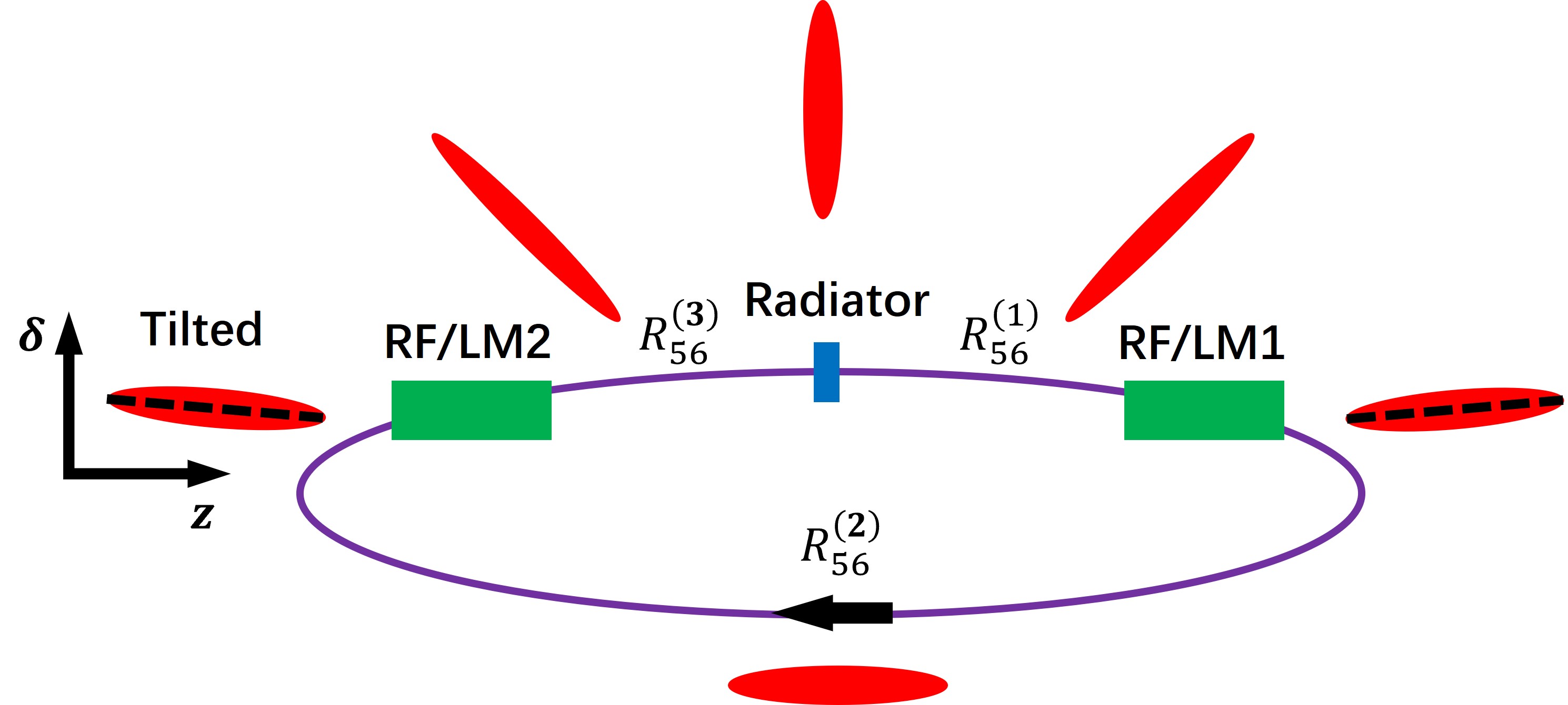
Figure 5: A schematic layout of a storage ring using two RF systems for longitudinal strong focusing and an example beam distribution evolution in longitudinal phase space.

We divide the ring into five sections from the transfer matrix viewpoint, i.e., three longitudinal drifts ($R_{56}$) and two longitudinal quadrupole kicks ($h$), with the linear transfer matrices given by

$${\bf T}_{\text{D1}}=\left(\begin{matrix}1&R_{56}^{(1)}\\ 0&1\end{matrix}\right),\ {\bf T}_{\text{RF1}}=\left(\begin{matrix}1&0\\ h_{1}&1\end{matrix}\right),\ {\bf T}_{\text{D2}}=\left(\begin{matrix}1&R_{56}^{(2)}\\ 0&1\end{matrix}\right),$$ (59)

$${\bf T}_{\text{RF2}}=\left(\begin{matrix}1&0\\ h_{2}&1\end{matrix}\right),\ {\bf T}_{\text{D3}}=\left(\begin{matrix}1&R_{56}^{(3)}\\ 0&1\end{matrix}\right).$$

Then the one-turn map at the radiator center is

$${\bf M}_{\text{R}} ={\bf T}_{\text{D3}}{\bf T}_{\text{RF2}}{\bf T}_{\text{D2}}{\bf T}_{\text{RF1}}{\bf T}_{\text{D1}}.$$ (60)

For the generation of coherent radiation, we usually want the bunch length to reach its minimum at the radiator, then we need $\alpha_{z}=0$ at the radiator.

With the primary goal of presenting the principle, instead of a detailed design, here for simplicity we focus on one special case: $R_{56}^{(1)}=R_{56}^{(3)}$, $h_{1}=h_{2}=h$. The treatment of more general cases with different signs and magnitudes of $R_{56}^{(1)}$ and $R_{56}^{(3)}$ and $h_{1}$ and $h_{2}$ is similar, but the same-signed $R_{56}^{(1)}$ and $R_{56}^{(3)}$ might be easier for a real lattice to fulfill. For example if $R_{56}^{(1)},R_{56}^{(3)}>0$, a possible realization of them are chicanes.

For the special case of $R_{56}^{(1)}=R_{56}^{(3)}$, $h_{1}=h_{2}=h$, denote $\zeta_{1}\equiv 1+R_{56}^{(1)}h,\ \zeta_{2}\equiv 1+\frac{R_{56}^{(2)}}{2}h,$ we then have

$${\bf M}_{\text{R}}=\left(\begin{matrix}2\zeta_{1}\zeta_{2}-1&2\frac{\zeta_{1}^{2}\zeta_{2}-\zeta_{1}}{h}\\ 2h\zeta_{2}&2\zeta_{1}\zeta_{2}-1\end{matrix}\right).$$ (61)

The linear stability requires $|2\zeta_{1}\zeta_{2}-1|<1$ which means $0<\zeta_{1}\zeta_{2}<1$.

We remind the readers that the analysis above about LSF has been presented before in Ref. [8]. Now we try to go further to gain more insight. The longitudinal beta function at the radiator is

$$\beta_{z\text{R}}=\frac{2\frac{\zeta_{1}^{2}\zeta_{2}-\zeta_{1}}{h}}{\sin\Phi_{z}}=\bigg{|}\frac{2\frac{\zeta_{1}^{2}\zeta_{2}-\zeta_{1}}{h}}{2\sqrt{\zeta_{1}\zeta_{2}\left(1-\zeta_{1}\zeta_{2}\right)}}\bigg{|}=\frac{1}{|h|}\sqrt{\frac{\zeta_{1}\left(1-\zeta_{1}\zeta_{2}\right)}{\zeta_{2}}},$$ (62)

where $\Phi_{z}=2\pi\nu_{s}$ is the synchrotron phase advance per turn. The longitudinal beta function at the opposite of the radiator, from where to LM2 has an $R_{56}=\frac{R_{56}^{(2)}}{2}$, is

$$\beta_{z\text{RO}}=\frac{1}{|h|}\sqrt{\frac{\zeta_{2}\left(1-\zeta_{1}\zeta_{2}\right)}{\zeta_{1}}},$$ (63)

which can be obtained by switching $\zeta_{1}$ and $\zeta_{2}$ in the expression of $\beta_{z\text{R}}$ in Eq. (62). So we have

$$\frac{\beta_{z\text{RO}}}{\beta_{z\text{R}}}=\frac{\zeta_{2}}{\zeta_{1}}.$$ (64)

The longitudinal beta function at the LM1 and LM2 (here we name them as modulators) is

$$\beta_{z\text{M}}=\beta_{z\text{R}}+\frac{{R_{56}^{(1)}}^{2}}{\beta_{z\text{R}}}.$$ (65)

Assuming that $|\zeta_{1}|\ll 1$ for efficient bunch compression from the place of modulator to the place of radiator. Then the bunch compression ratio from that at the modulator to that at the radiator is

$$\frac{\sigma_{z\text{M}}}{\sigma_{z\text{R}}}=\sqrt{\frac{\beta_{z\text{M}}}{\beta_{z\text{R}}}}=\sqrt{1+\frac{{R_{56}^{(1)}}^{2}}{\beta_{z\text{R}}^{2}}}=\sqrt{\frac{\zeta_{1}-2\zeta_{1}\zeta_{2}+\zeta_{2}}{\zeta_{1}\left(1-\zeta_{1}\zeta_{2}\right)}}\approx\sqrt{\frac{\zeta_{2}}{\zeta_{1}\left(1-\zeta_{1}\zeta_{2}\right)}}=\frac{1}{|h|\beta_{z\text{R}}}.$$ (66)

Then the energy chirp strength required is

$$|h|\approx\frac{1}{\sqrt{\beta_{z\text{R}}\beta_{z\text{M}}}}=\frac{\sqrt{\epsilon_{z}/\beta_{z\text{M}}}}{\sqrt{\epsilon_{z}\beta_{z\text{R}}}}=\frac{\sqrt{\epsilon_{z}/\beta_{z\text{M}}}}{\sigma_{z\text{R}}}.$$ (67)

The above relation is similar to the theorems to be presented in Sec. 4 about transverse-longitudinal coupling-based bunch compression schemes which is the backbone of the GLSF scheme. We assume that in a LSF ring, the longitudinal emittance is dominantly from the ring dipoles. This assumption will be checked later to see if it is really the case. Further, we assume that average longitudinal beta function at the dipoles equals that at the modulator, i.e., $\langle\beta_{z}\rangle=\beta_{z\text{M}}$. Then the equilibrium longitudinal emittance from the balance of quantum excitation and radiation damping in a ring consists of iso-bending-magnets has the scaling

$$\epsilon_{z}=\frac{55}{96\sqrt{3}}\frac{\alpha_{F}{\lambdabar}_{e}^{2}\gamma^{5}}{\alpha_{L}}\frac{\langle\beta_{z}\rangle}{\rho_{\text{ring}}^{3}}2\pi\rho_{\text{ring}}\propto\gamma^{2}\frac{\beta_{z\text{M}}}{\rho_{\text{ring}}},$$ (68)

with $\alpha_{L}\approx\frac{U_{0}}{E_{0}}\approx C_{\gamma}\frac{E_{0}^{3}}{\rho_{\text{ring}}}$ used in the last step. Then, from the above result and Eq. (67) we have the required energy chirp strength in a LSF ring scaling

$$|h|\propto\frac{\gamma}{\sigma_{z\text{R}}\sqrt{\rho_{\text{ring}}}}.$$ (69)

$\sigma_{z\text{R}}$ is determined by our desired radiation wavelength. Therefore, given the beam energy and desired bunch length, to lower the required energy chirp strength in LSF, we should use as large $\rho_{\text{ring}}$ as possible which means as weak as bending magnet as possible. But of course we should also consider the total length of the bending magnets, which should be within a reasonable range. Also note that when the bending magnets in the ring are very weak, the assumption that the longitudinal emittance in a LSF ring is dominantly from them will fail.

For a Gaussian bunch, the bunching factor at frequency $\omega$ is given by $b(\omega)=\text{exp}\left[-\frac{\left(\frac{\omega}{c}\sigma_{z}\right)^{2}}{2}\right]$. For significant 13.5 nm-wavelength coherent EUV radiation generation, we may need $\sigma_{z\text{R}}\lesssim 4$ nm ($b_{\text{13.5 nm}}\gtrsim 0.18$). To increase the radiation power, we may need the radiator, which is assumed to be an undulator, has a large period number $N_{u}$ (for example $N_{u}=300$). To avoid significant bunch lengthening from the energy spread and the undulator $R_{56}=2N_{u}\lambda_{R}$, we then need $N_{u}\lambda_{R}\sigma_{\delta}\lesssim\sigma_{z\text{R}}$, which then requires the energy spread at the radiator $\sigma_{\delta\text{R}}\lesssim 1\times 10^{-3}$. So we need $\epsilon_{z}=\sigma_{z\text{R}}\sigma_{\delta\text{R}}\lesssim 4$ pm. Since in a LSF ring, we cannot make the optimal conditions Eq. (26) be satisfied in all the bending magnets, then a reasonable argument is that the real longitudinal emittance should be at least a factor of two larger than the theoretical minimum (similar to that given in Eq. (29)), which then requires

$$\epsilon_{z,\text{min}}\lesssim 2\ \text{pm}.$$ (70)

Then according to Eq. (28), if $E_{0}=600$ MeV, we need $\theta\lesssim\frac{2\pi}{59}$, which means 59 bending magnets are needed. Assuming the length of each isochronous cell containing a bending magnet is 3 m, then the arc section of such a ring has a length of about 177 m. Considering the straight section for beam injection/extraction, radiation energy loss compensation, and longitudinal strong focusing section, the circumference of such a ring is about 200 m.

For $\epsilon_{z}=4$ pm, to get $\sigma_{z\text{R}}\lesssim 4$ nm, we need

$$\beta_{z\text{R}}\lesssim 4\ \mu\text{m}.$$ (71)

From Eq. (67), to decrease energy chirp strength $h$, we should apply as large $\beta_{z\text{M}}$ as possible since $\beta_{z0}\propto\rho$ with $\theta$ given. Therefore, we will choose a large (but acceptable) bending radius for the dipoles in the ring. If $\rho=10$ m ($B_{0}=0.2$ T and bending magnet total length 62.8 m), then the longitudinal beta function at the dipole center required to reach the practical theoretical minimum longitudinal emittance (see Eqs. (29) and (30)) is $\beta_{z0}=\frac{\sqrt{210}}{2520}\rho\theta^{3}=69.5\ \mu$m. Then we may let

$$\beta_{z\text{M}}\approx 2\beta_{z0}\approx 139\ \mu\text{m}.$$ (72)

Then the energy chirp strength required is

$$|h|\approx\frac{1}{\sqrt{\beta_{z\text{R}}\beta_{z\text{M}}}}\gtrsim 4.24\times 10^{4}\ \text{m}^{-1}.$$ (73)

According to Eq. (167) to be presented later about the laser modulator induced energy strength, if $E_{0}=600$ MeV, and for a modulator undulator with $\lambda_{u\text{M}}=8$ cm ($B_{0\text{M}}=1.13$ T), $L_{u\text{M}}=1.6$ m ($N_{u\text{M}}=20$), and for a laser with $\lambda_{L}=1064$ nm, to induced the required energy chirp strength, we need $P_{L}\approx 1$ GW. This is a large value and makes the optical enhancement cavity can only work in a low duty cycle pulsed mode, thus limiting the filling factor of microbunched electron beam in the ring, and thus limiting the average output EUV power.

We remind the readers that there is a subtle point in a LSF SSMB ring if we take the nonlinear sinusoidal modulation waveform into account, since the dynamic system is then strongly chaotic and requires careful parameters choice to ensure a large enough stable region for particle motion in the longitudinal phase space. More details in this respect can be found in Ref. [9].

Now for completeness of discussion, let us evaluate the contribution of modulator undulators to longitudinal emittance in this case, since there are also quantum excitation at the modulators. The quantum excitation contribution of two modulators to $\epsilon_{z}$ in a LSF ring is

$$\Delta\epsilon_{z\text{M}} =2\times\frac{55}{96\sqrt{3}}\frac{\alpha_{F}{\lambdabar}_{e}^{2}\gamma^{5}}{\alpha_{L}}\int_{0}^{L_{u\text{M}}}\frac{\beta_{z\text{M}}}{|\rho(s)|^{3}}ds$$ (74)

$$=2\times\frac{55}{96\sqrt{3}}\frac{\alpha_{F}{\lambdabar}_{e}^{2}\gamma^{5}}{\alpha_{L}}\frac{\beta_{z\text{M}}}{\rho_{M0}^{3}}\int_{0}^{L_{u\text{M}}}|\sin(k_{u}s)|^{3}ds$$

$$=2\times\frac{55}{96\sqrt{3}}\frac{\alpha_{F}{\lambdabar}_{e}^{2}\gamma^{5}}{\alpha_{L}}\frac{\beta_{z\text{M}}}{\rho_{M0}^{3}}\frac{4}{3\pi}L_{u\text{M}},$$

with

$$\alpha_{L}\approx\frac{U_{0}}{E_{0}}=C_{\gamma}\frac{E_{0}^{3}}{\rho_{\text{ring}}}=C_{\gamma}\times 0.2998B_{\text{ring}}[\text{T}]E_{0}^{2}[\text{GeV}]$$ (75)

with $C_{\gamma}=8.85\times 10^{-5}\frac{\text{m}}{\text{GeV}^{3}}$. Put in the numbers, we have

$$\Delta\epsilon_{z\text{M}}[\text{nm}] =8.9B_{\text{ring}}^{-1}[\text{T}]B_{0\text{M}}^{3}[\text{T}]\beta_{z\text{M}}[\text{m}]L_{u\text{M}}[\text{m}].$$ (76)

In our example case, $B_{\text{ring}}=0.2$ T, $B_{0\text{M}}=1.13$ T, $\beta_{z\text{M}}=139\ \mu$m, $L_{u\text{M}}=1.6$ m, we have

$$\Delta\epsilon_{z\text{M}}=14.3\ \text{pm},$$ (77)

which is even larger than the desired 4 pm longitudinal emittance, and therefore is unacceptable.

The above evaluation of longitudinal emittance contribution means we need to use a weaker or shorter modulator. We need to control the contribution of modulator to be $\Delta\epsilon_{z\text{M}}\lesssim 1$ pm since the ring dipoles will also contribute longitudinal emittance with a theoretical minimum about 2 pm. For example, we may choose to weaken the modulator field by more than a factor of two. If $\lambda_{u\text{M}}=0.15$ m and $B_{0\text{M}}=0.435$ T, $L_{u\text{M}}=1.5$ m ($N_{u\text{M}}=10$), then the contribution of two modulators to longitudinal emittance is

$$\Delta\epsilon_{z\text{M}}=0.76\ \text{pm},$$ (78)

which should be acceptable for a target total longitudinal emittance of 4 pm. But then to induce the desired energy chirp strength, we now need $P_{L}\approx 2$ GW.

Note that in this updated parameters choice, there is still one issue we need take care. In the evaluation of quantum excitation contribution of modulator to longitudinal emittance, we have implicitly assumed that the longitudinal beta function does not change inside it. This is not true strictly speaking. The undulator itself also has an $R_{56}=2N_{u}\lambda_{L}$. And the criterion whether the thin-lens approximation applies is to evaluate whether or not $|hR_{56}|\ll 1$, where $R_{56}$ is that of the undulator [8]. Here in this updated example, we have

$$hR_{56}=h2N_{u}\lambda_{L}=0.9$$ (79)

for the modulator, which means that the thin-lens kick approximation actually does not apply here. So more correctly we should use the thick-lens map of the modulator [8] to calculate the evolution of longitudinal beta function in the modulator, and then evaluate the contribution to longitudinal emittance.

LSF as analyzed above in principle can realize the desired nm bunch length and thus generate coherent EUV radiation. The main issue of such an EUV source is the required modulation laser power (GW level) is too high and makes the optical enhancement cavity can only work in a low duty cycle pulsed mode, thus limiting the average EUV output power. We remind the readers that the state-of-art stored laser power in an optical enhancement cavity is about 1 MW.

3.3 Generalized Longitudinal Strong Focusing

The above analysis on LWF and LSF then leads or forces us to the generalized longitudinal strong focusing (GLSF) scheme [10]. The basic idea of GLSF is to take advantage of the ultrasmall natural vertical emittance in a planar electron storage ring. More specifically, we will apply a partial transverse-longitudinal emittance exchange at the optical laser wavelength range for efficient microbunching generation. As shown in Fig. 4, the schematic setup of an GLSF ring is very similar to that of a LSF ring. But a sharp reader may notice that the laser modulator induced energy chirp strength in GLSF is much smaller than tat in the LSF, which means the required modulation laser power is smaller. Also one may wonder at first glance, the longitudinal phase space area is not conserved in the bunch compression or harmonic generation section of a GLSF ring. The fundamental physical law like Louisville’s theorem of course cannot be violated in a symplectic system. The reason for this apparent “contradiction” is that GLSF invokes 4D or 6D phase space dynamics as summarized in Tab. 1, and what are conserved is the eigen emittances, instead of the projected emittances. One may also note that in the GLSF scheme, the phase space rotation direction is reversed after radiator compared to that before the radiator, while in the LSF scheme this is not the case. In other words, in GLSF, we choose to make the upstream and downstream modulation cancel each other. In this sense, this setup is a special case of the reversible seeding scheme of SSMB [18]. The reason of doing this is that we want to make the system is transverse-longitudinal coupled only in a limited local place, so called GLSF section, such that we can maintain $\mathcal{H}_{y}=0$ at the majority place of the ring to keep the small vertical emittance of a planar uncoupled ring. Further, this cancellation of the nonlinear sinusoidal modulation waveforms will make the nonlinear dynamics of the ring easier to handle. To make the modulations perfectly cancel, we need the lattice between the upstream and down stream modulator to be an isochronous achromat. This reversible seeding makes the following decoupling of the system straightforward. All we need to do is to make the GLSF section an achromat, as the section from upstream modulator to downstream modulator is transparent to longitudinal dynamics. Another advantage of this reversible seeding setup is that it makes the bunch length at the modulator more flexible. It can be a short microbunned beam, or an a conventional RF-bunched beam, or even a coasting beam. Having explained the reason why we choose this reversible seeding setup for GLSF, we remind the readers that this however is not the only possible way to realize the GLSF scheme [10].

Now we want to appreciate in a more physical way why GLSF could be favored compared to LSF, in lowering the required modulation laser power? The key is that LSF has contribution of $\epsilon_{z}$ from both LSF section and the ring dipoles, while GLSF has only contribution of $\epsilon_{y}$ from the GLSF section, since $\mathcal{H}_{y}$ outside the GLSF section is zero. This is the key physical argument that why GLSF may require a smaller energy modulation compared to LSF, to realize the same desired bunch length at the radiator. Actually if the longitudinal emittance in LSF is only from the quantum excitation of LSF modulators, and the vertical emittance in GLSF is only from the quantum excitation of GLSF modulators, then GLSF and LSF are actually equivalent (only a different damping rate) in the requirement of energy modulation strength from single-particle dynamics perspective.

Now we explain the above argument more clearly with the help of formulas. As we will show in the following section, more specifically Eq. (93), in GLSF at best case we have

$$|h|=\frac{1}{\sqrt{\mathcal{H}_{y\text{R}}\mathcal{H}_{y\text{M}}}}=\frac{\sqrt{\epsilon_{y}/\mathcal{H}_{y\text{M}}}}{\sqrt{\epsilon_{y}\mathcal{H}_{y\text{R}}}}=\frac{\sqrt{\epsilon_{y}/\mathcal{H}_{y\text{M}}}}{\sigma_{z\text{R}}},$$ (80)

where $\mathcal{H}_{y}=\beta_{55}^{II}$ is defined in Ref. [14] and quantifies the contribution of vertical emittance to bunch length. One can appreciate the similarity of the above formula with Eq. (67) for the case of LSF. Therefore, GLSF will be advantageous to LSF in lowering the required energy modulation strength if

$$\frac{\epsilon_{y,\text{GLSF}}}{\mathcal{H}_{y\text{M},\text{GLSF}}}<\frac{\epsilon_{z,\text{LSF}}}{\beta_{z\text{M},\text{LSF}}}.$$ (81)

Now we compare the two schemes in a more quantitative way. We assume that the two schemes work at the same beam energy. As we will show in Sec. 7.1.1, in a GLSF SSMB ring and if we consider only single-particle dynamics, the dominant contribution of vertical emittance is from the quantum excitation of two modulators in the GLSF section, and we have

$$\epsilon_{y,\text{GLSF}} \approx 2\times\frac{55}{96\sqrt{3}}\frac{\alpha_{F}{\lambdabar}_{e}^{2}\gamma^{5}}{\alpha_{V,\text{GLSF}}}\frac{\mathcal{H}_{y\text{M},\text{GLSF}}}{\rho_{0\text{M}}^{3}}\frac{4}{3\pi}L_{u\text{M},\text{GLSF}},$$ (82)

with

$$\alpha_{V,\text{GLSF}}\approx\frac{U_{0}}{2E_{0}}\approx\frac{1}{2}C_{\gamma}\frac{E_{0}^{3}}{\rho_{\text{ring},\text{GLSF}}}.$$ (83)

We have assumed that the radiation loss in a GLSF ring is mainly from the bending magnets in the ring. While in LSF, we assume that the longitudinal emittance is mainly from the ring dipoles, and the average longitudinal beta function around the ring dipoles $\langle\beta_{z}\rangle=\beta_{z\text{M}}$. Then

$$\epsilon_{z,\text{LSF}}=\frac{55}{96\sqrt{3}}\frac{\alpha_{F}{\lambdabar}_{e}^{2}\gamma^{5}}{\alpha_{L,\text{LSF}}}\frac{\langle\beta_{z,\text{LSF}}\rangle}{\rho_{\text{ring},\text{LSF}}^{3}}2\pi\rho_{\text{ring},\text{LSF}},$$ (84)

with

$$\alpha_{L,\text{LSF}}\approx\frac{U_{0}}{E_{0}}\approx C_{\gamma}\frac{E_{0}^{3}}{\rho_{\text{ring},\text{LSF}}}.$$ (85)

Then Eq. (81) corresponds to

$$4\rho_{\text{ring},\text{GLSF}}\frac{1}{\rho_{0\text{M},\text{GLSF}}^{3}}\frac{4}{3\pi}L_{u\text{M},\text{GLSF}}<\rho_{\text{ring},\text{LSF}}\frac{1}{\rho_{\text{ring},\text{LSF}}^{3}}2\pi\rho_{\text{ring},\text{LSF}}.$$ (86)

The above condition should be straightforward to fulfill in practice. For example, if the bending magnet parameters are the same in both schemes, the above relation corresponds to

$$L_{u\text{M},\text{GLSF}}<\frac{3\pi^{2}}{8}\frac{\rho_{0\text{M},\text{GLSF}}^{3}}{\rho_{\text{ring}}^{2}},$$ (87)

which is easy to satisfy. So GLSF can be favored compared to LSF in lowering the required modulation laser power.

From nonlinear dynamics viewpoint, there is another possible advantage of GLSF compared to LSF. In GLSF scheme, as explained in the beginning of this section most likely we choose to make the two GLSF modulations cancel each other, while in LSF this is not the case. Therefore, considering the nonlinear modulation waveform, GLSF allows a more flexible $\sigma_{z}$ at the modulator, while in the longitudinal strong focusing scheme, the bunch length at the modulator should be much smaller than the modulation laser wavelength otherwise the particles will step into the chaotic region in phase space and their motion is unbounded.

So our tentative conclusion from the analysis in this section is: a LWF SSMB ring can be used to generate bunches with a couple of 10 nm bunch length, thus to generate coherent visible and infrared radiation. If we want to push the bunch length to an even shorter range, the required phase slippage factor of the ring will be too small from an engineering viewpoint. A LSF SSMB ring can create bunches with a bunch length at nm level, thus to generate coherent EUV radiation. However, the required modulation laser power is in GW level, and makes the optical enhancement cavity can only work at a low duty cycle pulsed mode, thus limiting the average output EUV radiation power. At present, a GLSF SSMB ring is the most promising among these three schemes to realize nm bunch length with a smaller modulation laser power compared to LSF SSMB, thus allowing higher average power EUV radiation generation. In the following sections, we will go into more details of the GLSF scheme, more specifically we will investigate the backbone of a GLSF SSMB storage ring, the transverse-longitudinal phase space coupling dynamics, in a systematic way. Finally, based on the investigation, we will present a solution of 1 kW-average-power EUV source based on GLSF SSMB.

4 Transverse-Longitudinal Coupling for Bunch Compression and Harmonic Generation

In this section, we present three theorems or inequalities that dictate the transverse-longitudinal coupling (TLC)-based bunch compression or harmonic generation schemes. These formal mathematical relations will be useful in our later more detailed design or parameters choice for an GLSF SSMB light source. If the initial bunch is longer than the modulation RF or laser wavelength, then compression of bunch or microbunch can just be viewed as a harmonic generation scheme. Therefore, in this paper, we will treat bunch compression and harmonic generation as the same thing in essence. Note that the theorems presented here are the generalization of that presented in Ref. [8] from 4D phase space to 6D phase space. It has been reported before in Ref. [19].

4.1 Problem Definition

Let us first define the problem we are trying to solve. We assume $\epsilon_{y}$ is the small eigenemittance we want to exploit. The case of using $\epsilon_{x}$ is similar. The schematic layout of a TLC-based bunch compression section is shown in Fig. 6. Suppose the beam at the entrance of the bunch compression section is $x$-$y$-$z$ decoupled, with its second moments matrix given by

Figure 6: A schematic layout of applying TLC dynamics for bunch compression.

$$\Sigma_{i}=\left(\begin{matrix}\epsilon_{x}\beta_{xi}&-\epsilon_{x}\alpha_{xi}&0&0&0&0\\ -\epsilon_{x}\alpha_{xi}&\epsilon_{x}{\gamma_{xi}}&0&0&0&0\\ 0&0&\epsilon_{y}\beta_{yi}&-\epsilon_{y}\alpha_{yi}&0&0\\ 0&0&-\epsilon_{y}\alpha_{yi}&\epsilon_{y}{\gamma_{yi}}&0&0\\ 0&0&0&0&\epsilon_{z}\beta_{zi}&-\epsilon_{z}\alpha_{zi}\\ 0&0&0&0&-\epsilon_{z}\alpha_{zi}&\epsilon_{z}{\gamma_{zi}}\\ \end{matrix}\right),$$ (88)

where $\alpha$, $\beta$ and $\gamma$ are the Courant-Snyder functions, the subscript _i means initial, and $\epsilon_{x}$, $\epsilon_{y}$ and $\epsilon_{z}$ are the eigenemittances of the beam corresponding to the horizontal, vertical and longitudinal mode, respectively. Note that eigenemittances are beam invariants with respect to linear symplectic transport. For the application of TLC for bunch compression, it means that the final bunch length at the exit or radiator $\sigma_{z\text{R}}$ depends only on the vertical emittance $\epsilon_{y}$ and not on the horizontal one $\epsilon_{x}$ and longitudinal one $\epsilon_{z}$.

We divide such a bunch compression section into three parts, with their symplectic transfer matrices given by

$${\bf M}_{1}=\left(\begin{matrix}r_{11}&r_{12}&r_{13}&r_{14}&0&r_{16}\\ r_{21}&r_{22}&r_{23}&r_{24}&0&r_{26}\\ r_{31}&r_{32}&r_{33}&r_{34}&0&r_{36}\\ r_{41}&r_{42}&r_{43}&r_{44}&0&r_{46}\\ r_{51}&r_{52}&r_{53}&r_{54}&1&r_{56}\\ 0&0&0&0&0&1\\ \end{matrix}\right),$$ (89)

$${\bf M}_{2}=\text{modulation kick map},$$

$${\bf M}_{3}=\left(\begin{matrix}R_{11}&R_{12}&R_{13}&R_{14}&0&R_{16}\\ R_{21}&R_{22}&R_{23}&R_{24}&0&R_{26}\\ R_{31}&R_{32}&R_{33}&R_{34}&0&R_{36}\\ R_{41}&R_{42}&R_{43}&R_{44}&0&R_{46}\\ R_{51}&R_{52}&R_{53}&R_{54}&1&R_{56}\\ 0&0&0&0&0&1\\ \end{matrix}\right),$$

where ${\bf M}_{1}$ representing “from entrance to modulator”, ${\bf M}_{2}$ representing “modulation kick” and ${\bf M}_{3}$ representing “modulator to radiator”. Note that ${\bf M}_{1}$ and ${\bf M}_{3}$ are in their general thick-lens form, and does not need to be $x$-$y$ decoupled. The transfer matrix from the entrance to the radiator is then

$${\bf T}={\bf M}_{3}{\bf M}_{2}{\bf M}_{1}.$$ (90)

From the problem definition, for $\sigma_{z\text{R}}$ to be independent of $\epsilon_{x}$ and $\epsilon_{z}$, we need

$$T_{51} =0,\ T_{52}=0,\ T_{55}=0,\ T_{56}=0.$$ (91)

4.2 Theorems and Proof

4.2.1 Theorems

Given the above problem definition, and assuming the modulation kick is a thin-lens one, we have three theorems which dictate the relation between the modulator kick strength with the optical functions at the modulator and radiator, respectively.
Theorem one: If

$${\bf M}_{2}=\left(\begin{matrix}1&0&0&0&0&0\\ 0&1&0&0&0&0\\ 0&0&1&0&0&0\\ 0&0&0&1&0&0\\ 0&0&0&0&1&0\\ 0&0&0&0&h&1\\ \end{matrix}\right),$$ (92)

which corresponds to the case of a normal RF or a TEM00 mode laser modulator, then

$$h^{2}\mathcal{H}_{y\text{M}}\mathcal{H}_{y\text{R}}\geq 1,$$ (93)

where the subscript M and R represent the place of modulator and radiator, respectively. Theorem two: If

$${\bf M}_{2}=\left(\begin{matrix}1&0&0&0&0&0\\ 0&1&0&0&0&0\\ 0&0&1&0&0&0\\ 0&0&0&1&t&0\\ 0&0&0&0&1&0\\ 0&0&t&0&0&1\\ \end{matrix}\right),$$ (94)

which corresponds to the case of a transverse deflecting (in $y$-dimension) RF or a TEM01 mode laser modulator or other schemes for angular modulation, then

$$t^{2}\beta_{y\text{M}}\mathcal{H}_{y\text{R}}\geq 1.$$ (95)

Theorem three: If

$${\bf M}_{2}=\left(\begin{matrix}1&0&0&0&0&0\\ 0&1&0&0&0&0\\ 0&0&1&0&k&0\\ 0&0&0&1&0&0\\ 0&0&0&0&1&0\\ 0&0&0&-k&0&1\\ \end{matrix}\right),$$ (96)

whose physical correspondence is not as straightforward as the previous two cases, then

$$k^{2}\gamma_{y\text{M}}\mathcal{H}_{y\text{R}}\geq 1.$$ (97)

4.2.2 Proof

Here we present the details for the proof of Theorem one. The proof of the other two is just similar. From the problem definition, for $\sigma_{z\text{R}}$ to be independent of $\epsilon_{x}$ and $\epsilon_{z}$, we need

$$T_{51} =r_{11}R_{51}+r_{21}R_{52}+r_{31}R_{53}+r_{41}R_{54}+r_{51}\left(hR_{56}+1\right)=0,$$ (98)

$$T_{52} =r_{12}R_{51}+r_{22}R_{52}+r_{32}R_{53}+r_{42}R_{54}+r_{52}\left(hR_{56}+1\right)=0,$$

$$T_{55} =hR_{56}+1=0,$$

$$T_{56} =r_{16}R_{51}+r_{26}R_{52}+r_{36}R_{53}+r_{46}R_{54}+r_{56}\left(hR_{56}+1\right)+R_{56}=0.$$

Under the above conditions, we have

$${\bf T}=\left(\begin{matrix}{\bf A}&{\bf B}&{\bf C}\\ {\bf D}&{\bf E}&{\bf F}\\ {\bf G}&{\bf H}&{\bf I}\end{matrix}\right),$$ (99)

with ${\bf A}\sim{\bf I}$ being $2\times 2$ submatrices of ${\bf T}$, and

$${\bf G}=\left(\begin{matrix}0&0\\ r_{51}h&r_{52}h\\ \end{matrix}\right),$$ (100)

$${\bf H}=\left(\begin{matrix}r_{13}R_{51}+r_{23}R_{52}+r_{33}R_{53}+r_{43}R_{54}&r_{14}R_{51}+r_{24}R_{52}+r_{34}R_{53}+r_{44}R_{54}\\ r_{53}h&r_{54}h\\ \end{matrix}\right),$$

$${\bf I}=\left(\begin{matrix}0&0\\ h&r_{56}h+1\\ \end{matrix}\right).$$

The bunch length squared at the modulator and the radiator are

$$\sigma_{z\text{M}}^{2} =\epsilon_{x}\frac{\left(\beta_{xi}r_{51}-\alpha_{xi}r_{52}\right)^{2}+r_{52}^{2}}{\beta_{xi}}+\epsilon_{y}\frac{\left(\beta_{yi}r_{53}-\alpha_{yi}r_{54}\right)^{2}+r_{54}^{2}}{\beta_{yi}}+\epsilon_{z}\left(\beta_{zi}-2\alpha_{zi}r_{56}+\gamma_{zi}r_{56}^{2}\right)$$ (101)

$$=\epsilon_{x}\mathcal{H}_{x\text{M}}+\epsilon_{y}\mathcal{H}_{y\text{M}}+\epsilon_{z}\beta_{z\text{M}},$$

$$\sigma_{z\text{R}}^{2} =\epsilon_{y}\frac{\left(\beta_{yi}T_{53}-\alpha_{yi}T_{54}\right)^{2}+T_{54}^{2}}{\beta_{yi}}=\epsilon_{y}\mathcal{H}_{y\text{R}}.$$

According to Cauchy-Schwarz inequality, we have

$$h^{2}\mathcal{H}_{y\text{M}}\mathcal{H}_{y\text{R}} =h^{2}\frac{\left[\left(\beta_{yi}r_{53}-\alpha_{yi}r_{54}\right)^{2}+r_{54}^{2}\right]}{\beta_{yi}}\frac{\left[\left(\beta_{yi}T_{53}-\alpha_{yi}T_{54}\right)^{2}+T_{54}^{2}\right]}{\beta_{yi}}$$ (102)

$$\geq\frac{h^{2}}{\beta_{yi}^{2}}\left[-\left(\beta_{yi}r_{53}-\alpha_{yi}r_{54}\right)T_{54}+r_{54}\left(\beta_{yi}T_{53}-\alpha_{yi}T_{54}\right)\right]^{2}$$

$$=\left(T_{53}r_{54}h-T_{54}r_{53}h\right)^{2}=\left(T_{53}T_{64}-T_{54}T_{63}\right)^{2}=|\text{det}({\bf H})|^{2}.$$

The equality holds when $\frac{-\left(\beta_{yi}r_{53}-\alpha_{yi}r_{54}\right)}{T_{54}}=\frac{r_{54}}{\left(\beta_{yi}T_{53}-\alpha_{yi}T_{54}\right)}.$ The symplecticity of ${\bf T}$ requires that ${\bf T}{\bf S}{\bf T}^{T}={\bf S}$, where ${\bf S}=\left(\begin{matrix}{\bf J}&0&0\\ 0&{\bf J}&0\\ 0&0&{\bf J}\end{matrix}\right)$ and ${\bf J}=\left(\begin{matrix}0&1\\ -1&0\end{matrix}\right),$ so we have

$$\left(\begin{matrix}{\bf A}{\bf J}{\bf A}^{T}+{\bf B}{\bf J}{\bf B}^{T}+{\bf C}{\bf J}{\bf C}^{T}&{\bf A}{\bf J}{\bf D}^{T}+{\bf B}{\bf J}{\bf E}^{T}+{\bf C}{\bf J}{\bf F}^{T}&{\bf A}{\bf J}{\bf G}^{T}+{\bf B}{\bf J}{\bf H}^{T}+{\bf C}{\bf J}{\bf I}^{T}\\ {\bf D}{\bf J}{\bf A}^{T}+{\bf E}{\bf J}{\bf B}^{T}+{\bf F}{\bf J}{\bf C}^{T}&{\bf D}{\bf J}{\bf D}^{T}+{\bf E}{\bf J}{\bf E}^{T}+{\bf F}{\bf J}{\bf F}^{T}&{\bf D}{\bf J}{\bf G}^{T}+{\bf E}{\bf J}{\bf H}^{T}+{\bf F}{\bf J}{\bf I}^{T}\\ {\bf G}{\bf J}{\bf A}^{T}+{\bf H}{\bf J}{\bf B}^{T}+{\bf I}{\bf J}{\bf C}^{T}&{\bf G}{\bf J}{\bf D}^{T}+{\bf H}{\bf J}{\bf E}^{T}+{\bf I}{\bf J}{\bf F}^{T}&{\bf G}{\bf J}{\bf G}^{T}+{\bf H}{\bf J}{\bf H}^{T}+{\bf I}{\bf J}{\bf I}^{T}\\ \end{matrix}\right)={\bf S}.$$ (103)

According to Eq. (100), we have ${\bf G}{\bf J}{\bf G}^{T}=\left(\begin{matrix}0&0\\ 0&0\end{matrix}\right)$, ${\bf I}{\bf J}{\bf I}^{T}=\left(\begin{matrix}0&0\\ 0&0\end{matrix}\right)$. Therefore,

$${\bf H}{\bf J}{\bf H}^{T}={\bf J},$$ (104)

which means ${\bf H}$ is also a symplectic matrix. So we have $\text{det}({\bf H})=1.$ The theorem is thus proven.

4.3 Dragt’s Minimum Emittance Theorem

Theorem one in Eq. (93) can also be expressed as

$$|h|\geq\frac{\epsilon_{y}}{\sqrt{\epsilon_{y}\mathcal{H}_{y\text{M}}}\sqrt{\epsilon_{y}\mathcal{H}_{y\text{R}}}}=\frac{\epsilon_{y}}{\sigma_{zy\text{M}}\sigma_{z\text{R}}}.$$ (105)

Note that in the above formula, $\sigma_{zy\text{M}}$ means the bunch length at the modulator contributed from the vertical emittance $\epsilon_{y}$. So given a fixed $\epsilon_{y}$ and desired $\sigma_{z\text{R}}$, a smaller $h$, i.e., a smaller RF acceleration gradient or modulation laser power ($P_{L}\propto|h|^{2}$), means a larger $\mathcal{H}_{y\text{M}}$, thus a longer $\sigma_{zy\text{M}}$, is needed. As $|h|\sigma_{z\text{M}}$ quantifies the energy spread introduced by the modulation kick, we thus also have

$$\sigma_{z\text{R}}\sigma_{\delta\text{R}}\geq\epsilon_{y}.$$ (106)

Similarly for Theorem two and three, we have

$$|t| \geq\frac{\epsilon_{y}}{\sigma_{y\beta\text{M}}\sigma_{z\text{R}}},$$ (107)

and

$$|k| \geq\frac{\epsilon_{y}}{\sigma_{y^{\prime}\beta\text{M}}\sigma_{z\text{R}}},$$ (108)

respectively, and also Eq. (106). Note that in the above formulas, the vertical beam size or divergence at the modulator contains only the vertical betatron part, i.e., that from the vertical emittance $\epsilon_{y}$.

Equation (106) is actually a manifestation of the classical uncertainty principle [20], which states that

$$\Sigma_{11}\Sigma_{22} \geq\epsilon_{\text{min}}^{2},$$ (109)

$$\Sigma_{33}\Sigma_{44} \geq\epsilon_{\text{min}}^{2},$$

$$\Sigma_{55}\Sigma_{66} \geq\epsilon_{\text{min}}^{2},$$

in which $\epsilon_{\text{min}}$ is the minimum one among the three eigen emittances $\epsilon_{I,II,III}$. In our bunch compression case, we assume that $\epsilon_{y}$ is the smaller one compared to $\epsilon_{z}$.

Actually there is a stronger inequality compared to the classical uncertainty principle, i.e., the minimum emittance theorem [20], which states that the projected emittance cannot be smaller than the minimum one among the three eigen emittances,

$$\epsilon_{x,\text{pro}}^{2}=\Sigma_{11}\Sigma_{22}-\Sigma_{12}^{2} \geq\epsilon_{\text{min}}^{2},$$ (110)

$$\epsilon_{y,\text{pro}}^{2}=\Sigma_{33}\Sigma_{44}-\Sigma_{34}^{2} \geq\epsilon_{\text{min}}^{2},$$

$$\epsilon_{z,\text{pro}}^{2}=\Sigma_{55}\Sigma_{66}-\Sigma_{56}^{2} \geq\epsilon_{\text{min}}^{2}.$$

4.4 Theorems Cast in Another Form

As another way to appreciate the result, here we cast the theorems in a form using the generalized beta functions as introduced in Ref. [14]. According to definition, we have

$$\beta_{y}\equiv\beta_{33}^{II},\ \gamma_{y}\equiv\beta_{44}^{II},\ \mathcal{H}_{y}\equiv\beta_{55}^{II}.$$ (111)

Theorem one: If ${\bf M}_{2}$ is as shown in Eq. (92), then

$$M_{65}^{2}(\text{Mod})\beta_{55}^{II}(\text{Mod})\beta_{55}^{II}(\text{Rad})\geq 1,$$ (112)

where $M_{65}$ is the ₆₅ matrix term of ${\bf M}_{2}$, i.e., $h$. In this section, we use brackets to denote the location, with Ent, Mod and Rad meaning entrance, modulator and radiator, respectively.
Theorem two: If ${\bf M}_{2}$ is as shown in Eq. (94), then

$$M_{63}^{2}(\text{Mod})\beta_{33}^{II}(\text{Mod})\beta_{55}^{II}(\text{Rad})\geq 1.$$ (113)

Theorem three: If ${\bf M}_{2}$ is as shown in Eq. (96), then

$$M_{64}^{2}(\text{Mod})\beta_{44}^{II}(\text{Mod})\beta_{55}^{II}(\text{Rad})\geq 1.$$ (114)

At the entrance, the generalized Twiss matrix corresponding to eigen mode $I$ is

$${\bf T}_{I}(\text{Ent})=\left(\begin{matrix}\beta_{xi}&-\alpha_{xi}&0&0&0&0\\ -\alpha_{xi}&\gamma_{xi}&0&0&0&0\\ 0&0&0&0&0&0\\ 0&0&0&0&0&0\\ 0&0&0&0&0&0\\ 0&0&0&0&0&0\\ \end{matrix}\right),$$ (115)

and similar expressions for ${\bf T}_{II,III}(\text{Ent})$, with $x$ replaced by $y,z$ and the location of the $2\times 2$ matrix shifted in the diagonal direction. Then

$$\beta_{33}^{II}(\text{Mod})=\frac{\left(\beta_{yi}r_{33}-\alpha_{yi}r_{34}\right)^{2}+r_{34}^{2}}{\beta_{yi}},$$ (116)

$$\beta_{44}^{II}(\text{Mod})=\frac{\left(\beta_{yi}r_{43}-\alpha_{yi}r_{44}\right)^{2}+r_{44}^{2}}{\beta_{yi}},$$ (117)

$$\beta_{55}^{II}(\text{Mod})=\frac{\left(\beta_{yi}r_{53}-\alpha_{yi}r_{54}\right)^{2}+r_{54}^{2}}{\beta_{yi}},$$ (118)

$$\beta_{55}^{I}(\text{Rad})=\frac{\left(\beta_{xi}T_{51}-\alpha_{xi}T_{52}\right)^{2}+T_{52}^{2}}{\beta_{xi}},$$ (119)

$$\beta_{55}^{II}(\text{Rad})=\frac{\left(\beta_{yi}T_{53}-\alpha_{yi}T_{54}\right)^{2}+T_{54}^{2}}{\beta_{yi}},$$ (120)

$$\beta_{55}^{III}(\text{Rad})=\frac{\left(\beta_{zi}T_{55}-\alpha_{zi}T_{56}\right)^{2}+T_{56}^{2}}{\beta_{zi}}.$$ (121)

For $\sigma_{z\text{R}}$ to be independent of $\epsilon_{x}$ and $\epsilon_{z}$, we need $\beta_{55}^{I}(\text{Rad})=0$ and $\beta_{55}^{III}(\text{Rad})=0$, which then lead to Eq. (91). And the following proof procedures are the same as that shown in the above Sec. 4.2.2.

5 Energy Modulation-Based Coupling Schemes

Now we conduct more in-depth analysis of the TLC-based bunch compression or microbunching generation schemes. We group these schemes into two categories, i.e., energy modulation-based and angular modulation-based schemes. They corresponds to the case of Theorem One and Two presented in last section. In this section, we focus on energy modulation-based coupling schemes, and next section is dedicated to angular modulation-based schemes. The physical realization corresponds to the case of Theorem Three is not that straightforward compared to the cases of Theorem One and Two, and we do not expand its discussion it in this paper.

5.1 Bunching Factor

5.1.1 Formal Analysis

First we derive the bunching factor formula of energy-modulation based TLC microbunching schemes. The mathematical model is formulated as follows.
Particle state vector:

$${\bf X}=\left(\begin{matrix}x&x^{\prime}&y&y^{\prime}&z&\delta\end{matrix}\right)^{T}.$$ (122)

Initial Gaussian beam distribution at the modulator:

$$\rho_{0}({\bf X}) =\frac{1}{(2\pi)^{3}\sqrt{\text{Det}({\bf\Sigma_{0}})}}\text{exp}\left(-\frac{1}{2}{\bf X}^{T}{\bf\Sigma_{0}^{-1}}{\bf X}\right),$$ (123)

with ${\bf\Sigma}=\langle{\bf X}{\bf X}^{T}\rangle$ the second moments of the matrix.
Lumped laser-induced energy modulation:

$$\delta=\delta+A\sin(k_{L}z).$$ (124)

Beam evolution after modulation:

$${\bf X}={\bf R}{\bf X},$$ (125)

where ${\bf R}$ is the transfer matrix of the magnet lattice, which could be a single-pass one like a linear accelerator or a multi-pass one like a storage ring. Note that ${\bf R}$ here can be 6D general coupled.
 
We want to know the final beam distribution in phase space and functions defined based on the distribution. For example, we can define a generalized bunching factor at wavenumber $k$:

$$b(k)=\int\rho({\bf X})e^{-ik{\bf W}{\bf X}}d{\bf X}\\$$ (126)

where ${\bf W}\equiv\left(\begin{matrix}w_{1}&w_{2}&w_{3}&w_{4}&w_{5}&w_{6}\end{matrix}\right)$. For example, if ${\bf W}\equiv\left(\begin{matrix}0&0&0&0&1&0\end{matrix}\right)$, we arrive at the classical definition of bunching factor

$$b(k)=\int_{-\infty}^{\infty}\rho(z)e^{-ikz}dz,$$ (127)

which can be used to quantify the ability of a particle beam with longitudinal charge density distribution $\rho(z)$ to generate coherent radiaton at wavenumber $k$. If ${\bf W}\equiv\left(\begin{matrix}\sin\theta\cos\varphi&0&\sin\theta\sin\varphi&0&1&0\end{matrix}\right)$, we arrive at the angular-spectral bunching factor [8]

$$b(\theta,\varphi,k)=\int_{-\infty}^{\infty}\int_{-\infty}^{\infty}\int_{-\infty}^{\infty}\rho(x,y,z)e^{-ik\left(x\sin\theta\cos\varphi+y\sin\theta\sin\varphi+z\right)}dxdydz,$$ (128)

which can be used to study the impact of particle transverse coordinates on coherent radiation. In this paper, we will mainly discuss the case of classical bunching factor definition, i.e., Eq. (127). But our analysis of generalized bunching factor below is general and can be applied to more involved situation.
 
Denote:

$${\bf W} \equiv\left(\begin{matrix}w_{1}&w_{2}&w_{3}&w_{4}&w_{5}&w_{6}\end{matrix}\right),$$ (129)

$${\bf U}_{\frac{pk_{L}}{k}} \equiv\left(\begin{matrix}0&0&0&0&\frac{pk_{L}}{k}&0\end{matrix}\right),$$

$${\bf M}_{\frac{pk_{L}}{k}} \equiv{\bf W}{\bf R}-{\bf U}_{\frac{pk_{L}}{k}},$$

$${\bf R}_{i6} =\left(\begin{matrix}R_{16}&R_{26}&R_{36}&R_{46}&R_{56}&R_{66}\end{matrix}\right)^{T}.$$

Then the generalized bunching factor at wavenumber $k$ at the final location is

$$b(k) =\int\rho_{f}({\bf X})e^{-ik{\bf W}{\bf X}}d{\bf X}$$ (130)

$$=\int\rho_{m+}({\bf X})e^{-ik{\bf WR}{\bf X}}d{\bf X}$$

$$=\int\rho_{0}({\bf X})e^{-ik\left({\bf WR}{\bf X}+{\bf W}{\bf R}_{i6}A\sin(k_{L}z)\right)}d{\bf X}$$

$$=\sum_{p=-\infty}^{\infty}J_{p}\left(-k{\bf W}{\bf R}_{i6}A\right)\text{exp}\left(-\frac{k^{2}}{2}{\bf M}_{\frac{pk_{L}}{k}}{\bf\Sigma}_{0}{\bf M}_{\frac{pk_{L}}{k}}^{T}\right),$$

where $\rho_{0}({\bf X})$, $\rho_{m+}({\bf X})$, and $\rho_{f}({\bf X})$ mean the beam distribution at the beginning, right after the energy modulation and the final point, respectively. $J_{p}$ is the $p$-th order Bessel function of the first kind. Jacobi-Anger identity $e^{ix\sin(k_{L}z)}=\sum_{n=-\infty}^{\infty}e^{ink_{L}z}J_{n}[x]$ has been used in the above derivation.
 
The above result is the most general bunching factor formula for one-stage laser-induced energy modulation-based microbunching schemes. It applies for arbitrary coupled lattice.
 
Using the real and imaginary generalized beta functions and Twiss matrices introduced in Ref. [14], we can write

$${\bf M}_{\frac{pk_{L}}{k}}{\bf\Sigma}_{0}{\bf M}_{\frac{pk_{L}}{k}}^{T} =\sum_{\kappa=I,II,III}\epsilon_{\kappa}\left({\bf W}{\bf R}{\bf T}_{\kappa}{\bf R}^{T}{\bf W}^{T}-2{\bf W}{\bf R}{\bf T}_{\kappa}{\bf U}_{\frac{pk_{L}}{k}}^{T}+{\bf U}_{\frac{pk_{L}}{k}}{\bf T}_{\kappa}{\bf U}_{\frac{pk_{L}}{k}}^{T}\right),$$ (131)

where ${\bf T}_{\kappa}$ is the generalized real Twiss matrix of the $\kappa$-th eigenmode right before the modulation.

5.1.2 HGHG

In the following discussion, we will let ${\bf W}=\left(\begin{matrix}0&0&0&0&1&0\end{matrix}\right)$, then

$${\bf W}{\bf R_{i6}} =R_{56},$$ (132)

$${\bf M}_{\frac{pk_{L}}{k}} =\left(\begin{matrix}R_{51}&R_{52}&R_{53}&R_{54}&R_{55}-\frac{pk_{L}}{k}&R_{56}\end{matrix}\right).$$

If further $R_{51}=0$, $R_{52}=0$, $R_{53}=0$, $R_{54}=0$ and $R_{55}=1$, and the initial beam is transverse-longitudinal decoupled and has an upright distribution in the longitudinal phase space, then

$$b(k) =\sum_{p=-\infty}^{\infty}J_{p}\left(-kR_{56}A\right)\text{exp}\left(-\frac{k^{2}}{2}\left[\left(1-\frac{pk_{L}}{k}\right)^{2}\sigma_{z0}^{2}+\left(R_{56}\sigma_{\delta 0}\right)^{2}\right]\right).$$ (133)

If the initial bunch length is much longer than the laser wavelength, i.e., $\sigma_{z0}\gg\lambda_{L}$, the above exponential terms will be non-zero only when $1-\frac{pk_{L}}{k}=0$, which means there is only bunching at the laser harmonics. Therefore, we have the bunching factor at the $n$-th ($n$ being integer) laser harmonic

$$b_{n}=b(nk_{L}) =J_{n}(-nk_{L}{R}_{56}A)\text{exp}\left[-\frac{\left(nk_{L}R_{56}\sigma_{\delta 0}\right)^{2}}{2}\right].$$ (134)

This corresponds to the case of high-gain harmonic-generation (HGHG) [21]. When $n\gg 1$, the maximal value of $J_{n}$ is achieved when its argument is equal to $n+0.81n^{1/3}$ and the value is about $0.67/n^{1/3}$. For large $n$, we have $n\gg 0.81n^{1/3}$, so roughly we need $k_{L}{R}_{56}A\sim 1$ to make the Bessel function term in Eq. (134) reaches the maximum. To make the exponential term not too small, which means $nk_{L}R_{56}\sigma_{\delta 0}\lesssim 1$, we then need $A\gtrsim n\sigma_{\delta 0}$. So generally if we want to realize $n$-th laser harmonic bunching in HGHG, we need an energy modulation strength a factor of $n$ larger than the natural energy spread. This limits the harmonic number that can be reached by a single-stage HGHG, since a too large energy spread will degrade the lasing process in a free-electron laser (FEL). In addition, it also means a large modulation laser power is needed, which is not favorable for the application in SSMB.

5.1.3 TLC-based Microbunching

Now let us consider the case of nonzero $R_{51,2,3,4}$. If ${\bf W}\equiv\left(\begin{matrix}0&0&0&0&1&0\end{matrix}\right),$ and for a TLC-based microbunching scheme, we require that in the final bunching factor formula, for a specific $p$ only one transverse emittance contributes to the exponential term in Eq. (130), $\text{exp}\left(-\frac{k^{2}}{2}{\bf M}_{\frac{pk_{L}}{k}}{\bf\Sigma}_{0}{\bf M}_{\frac{pk_{L}}{k}}^{T}\right)$. The motivation of doing this is that if one of the transverse eigenemittance is very small, then we can realize very high harmonic number with a small energy modulation strength. Since in a planar electron storage ring, the vertical beam emittance is naturally quite small, so we can take advantage of $y$-$z$ coupling for efficient bunch compression or harmonic generation. This is the basic idea behind the generalized longitudinal strong focusing scheme [10].

In the below we use $y$-$z$ coupling as an example for the analysis and ignore the $x$-dimension. The analysis for $x$-$z$ coupling is similar. If $R_{51}=0$, $R_{52}=0$, $R_{55}=1$, $R_{66}=1$, then

$${\bf W}{\bf R_{i6}} =R_{56},$$ (135)

$${\bf M}_{\frac{pk_{L}}{k}} =\left(\begin{matrix}0&0&R_{53}&R_{54}&1-\frac{pk_{L}}{k}&R_{56}\end{matrix}\right).$$

Then the bunching factor at the $n$-th laser harmonic is

$$b_{n} =\sum_{p=-\infty}^{\infty}J_{p}\left(-pk_{L}R_{56}A\right)\text{exp}\left[-\frac{(nk_{L})^{2}}{2}\left({\bf M}_{\frac{p}{n}}{\bf T}_{II}{\bf M}_{\frac{p}{n}}^{T}+{\bf M}_{\frac{p}{n}}{\bf T}_{III}{\bf M}_{\frac{p}{n}}^{T}\right)\right].$$ (136)

We then require

$${\bf M}_{\frac{p}{n}}{\bf T}_{III}{\bf M}_{\frac{p}{n}}^{T}\Bigg{|}_{\frac{p}{n}=1} =\left({\bf R}{\bf T}_{III}{\bf R}^{T}-2{\bf R}{\bf T}_{III}+{\bf T}_{III}\right)_{55}=0.$$ (137)

Using the real and imaginary generalized beta functions and Twiss matrices introduced in Ref. [14], the above relation can be casted into

$$R_{53}^{2}\beta_{33}^{III}+R_{54}^{2}\beta_{44}^{III}+R_{56}^{2}\beta_{66}^{III}+2R_{53}R_{54}\beta_{34}^{III}+2R_{53}R_{56}\beta_{36}^{III}+2R_{54}R_{56}\beta_{46}^{III}=0.$$ (138)

If the generalized Twiss matrices of three eigenmodes right before the modulation are given by

$${\bf T}_{I} =\left(\begin{array}[]{cccccc}\beta_{x}&-\alpha_{x}&0&0&-\alpha_{x}D_{x}-\beta_{x}D_{x}^{\prime}&0\\ -\alpha_{x}&\gamma_{x}&0&0&\gamma_{x}D_{x}+\alpha_{x}D_{x}^{\prime}&0\\ 0&0&0&0&0&0\\ 0&0&0&0&0&0\\ -\alpha_{x}D_{x}-\beta_{x}D_{x}^{\prime}&\gamma_{x}D_{x}+\alpha_{x}D_{x}^{\prime}&0&0&\mathcal{H}_{x}&0\\ 0&0&0&0&0&0\\ \end{array}\right),$$ (139)

$${\bf T}_{II} =\left(\begin{array}[]{cccccc}0&0&0&0&0&0\\ 0&0&0&0&0&0\\ 0&0&\beta_{y}&-\alpha_{y}&-\alpha_{y}D_{y}-\beta_{y}D_{y}^{\prime}&0\\ 0&0&-\alpha_{y}&\gamma_{y}&\gamma_{y}D_{y}+\alpha_{y}D_{y}^{\prime}&0\\ 0&0&-\alpha_{y}D_{y}-\beta_{y}D_{y}^{\prime}&\gamma_{y}D_{y}+\alpha_{y}D_{y}^{\prime}&\mathcal{H}_{y}&0\\ 0&0&0&0&0&0\\ \end{array}\right),$$ (140)

$${\bf T}_{III} =\left(\begin{array}[]{cccccc}\gamma_{z}D_{x}^{2}&\gamma_{z}D_{x}D_{x}^{\prime}&\gamma_{z}D_{x}D_{y}&\gamma_{z}D_{x}D_{y}^{\prime}&-\alpha_{z}D_{x}&\gamma_{z}D_{x}\\ \gamma_{z}D_{x}D_{x}^{\prime}&\gamma_{z}D_{x}^{\prime 2}&\gamma_{z}D_{x}^{\prime}D_{y}&\gamma_{z}D_{x}^{\prime}D_{y}^{\prime}&-\alpha_{z}D_{x}^{\prime}&\gamma_{z}D_{x}^{\prime}\\ \gamma_{z}D_{x}D_{y}&\gamma_{z}D_{x}^{\prime}D_{y}&\gamma_{z}D_{y}^{2}&\gamma_{z}D_{y}D_{y}^{\prime}&-\alpha_{z}D_{y}&\gamma_{z}D_{y}\\ \gamma_{z}D_{x}D_{y}^{\prime}&\gamma_{z}D_{x}^{\prime}D_{y}^{\prime}&\gamma_{z}D_{y}D_{y}^{\prime}&\gamma_{z}D_{y}^{\prime 2}&-\alpha_{z}D_{y}^{\prime}&\gamma_{z}D_{y}^{\prime}\\ -\alpha_{z}D_{x}&-\alpha_{z}D_{x}^{\prime}&-\alpha_{z}D_{y}&-\alpha_{z}D_{y}^{\prime}&\beta_{z}&-\alpha_{z}\\ \gamma_{z}D_{x}&\gamma_{z}D_{x}^{\prime}&\gamma_{z}D_{y}&\gamma_{z}D_{y}^{\prime}&-\alpha_{z}&\gamma_{z}\\ \end{array}\right),$$ (141)

and further assuming that at the modulation point we have $D_{x}=0$ and $D_{x}^{\prime}=0$, then Eq. (138) can be casted into

$$\gamma_{z}\left(R_{53}D_{y}+R_{54}D_{y}^{\prime}+R_{56}\right)^{2}=0\Rightarrow R_{53}D_{y}+R_{54}D_{y}^{\prime}+R_{56}=0.$$ (142)

This relation means the final coordinate $z$ does not depend on the initial energy deviation $\delta$. Under the above condition, then

$${\bf M}_{\frac{p}{n}}{\bf T}_{III}{\bf M}_{\frac{p}{n}}^{T} =\left(1-\frac{p}{n}\right)^{2}\beta_{z\text{M}},$$ (143)

and

$${\bf M}_{\frac{p}{n}}{\bf T}_{II}{\bf M}_{\frac{p}{n}}^{T}$$ (144)

$$=\frac{\gamma_{y}\left((n-p)D_{y}+nR_{54}\right){}^{2}+2\alpha_{y}\left((n-p)D_{y}+nR_{54}\right)\left((n-p)D_{y}^{\prime}-nR_{53}\right)+\beta_{y}\left((n-p)D_{y}^{\prime}-nR_{53}\right){}^{2}}{n^{2}}$$

$$=R_{53}^{2}\beta_{y}-2R_{54}R_{53}\alpha_{y}+R_{54}^{2}\gamma_{y}+\left(1-\frac{p}{n}\right)^{2}\left(\gamma_{y}D_{y}^{2}+2\alpha_{y}D_{y}D_{y}^{\prime}+\beta_{y}D_{y}^{\prime 2}\right)$$

$$\ \ \ \ +2\left(1-\frac{p}{n}\right)\left(\gamma_{y}R_{54}D_{y}-\alpha_{y}R_{53}D_{y}+\alpha_{y}R_{54}D_{y}^{\prime}-\beta_{y}R_{53}D_{y}^{\prime}\right)$$

$$=\mathcal{H}_{y\text{R}}+\left(1-\frac{p}{n}\right)^{2}\mathcal{H}_{y\text{M}}+2\left(1-\frac{p}{n}\right)\left(\gamma_{y}R_{54}D_{y}-\alpha_{y}R_{53}D_{y}+\alpha_{y}R_{54}D_{y}^{\prime}-\beta_{y}R_{53}D_{y}^{\prime}\right).$$

Note that $\left(\gamma_{y}R_{54}D_{y}-\alpha_{y}R_{53}D_{y}+\alpha_{y}R_{54}D_{y}^{\prime}-\beta_{y}R_{53}D_{y}^{\prime}\right)$ can also be expressed more elegantly as $\sqrt{\mathcal{H}_{y\text{R}}\mathcal{H}_{y\text{M}}}\cos(\Delta\psi_{\mathcal{H}})$. We will continue this formal analysis and presente it elsewhere. Then the bunching factor at the $n$-th laser harmonic at the final point is

$$b_{n} =\sum_{p=-\infty}^{\infty}J_{p}\left(-pk_{L}R_{56}A\right)\text{exp}\left[-\frac{(nk_{L})^{2}}{2}\epsilon_{y}\mathcal{H}_{y\text{R}}\right]$$ (145)

$$\ \ \ \ \text{exp}\left[-\frac{k_{L}^{2}}{2}\left(n-p\right)^{2}\left(\epsilon_{y}\mathcal{H}_{y\text{M}}+\epsilon_{z}\beta_{z\text{M}}\right)\right]$$

$$\ \ \ \ \text{exp}\left[-\frac{k_{L}^{2}}{2}2n\left(n-p\right)\epsilon_{y}\left(\gamma_{y}R_{54}D_{y}-\alpha_{y}R_{53}D_{y}+\alpha_{y}R_{54}D_{y}^{\prime}-\beta_{y}R_{53}D_{y}^{\prime}\right)\right].$$

We have proven in the last section there is a fundamental inequality dictating the energy chirp strength $h$ and $\mathcal{H}_{y}$ at the modulator and radiator, respectively, i.e., Eq. (105). Basically, given the vertical emittance and desired linear bunch length at radiator, to lower the energy chirp strength, we need to lengthen the bunch at the modulator. If the initial bunch is shorter than the modulation laser wavelength, then according to Eq. (145), a bunch lengthening at the modulator means a bunching factor drop at the radiator as can be seen from the second exponential term. The physical picture of this is given in Fig. 7. For more discussion on this point, refer to Refs. [8] and [25].

When $k_{L}^{2}\left(\epsilon_{y}\mathcal{H}_{y\text{M}}+\epsilon_{z}\beta_{z\text{M}}\right)\gg 1$ which means the bunch length at the modulation point is much longer than the laser wavelength, then there is only one term non-vanishing in the above summation, i.e., the term with $p=n$. Then

$$b_{n} =J_{n}\left(-nk_{L}R_{56}A\right)\text{exp}\left[-\frac{(nk_{L})^{2}}{2}\epsilon_{y}\mathcal{H}_{y\text{R}}\right].$$ (146)

This is the bunching factor formula for TLC-based microbunching schemes like phase-merging enhanced harmonic generation (PEHG) [22, 23] and angular dispersion-induced microbunching (ADM) [24] to be introduced soon. It applies when the initial bunch length is much longer than the modulation laser wavelength.

Here we remind the readers that there is an extra term in Eq. (145) compared to the bunching factor formula for a premicrobunches beam presented in Refs. [8] and [25], i.e.,

$$b_{n} =\sum_{p=-\infty}^{\infty}J_{p}\left(-pk_{L}R_{56}A\right)\text{exp}\left[-\frac{(nk_{L})^{2}}{2}\epsilon_{y}\mathcal{H}_{y\text{R}}\right]$$ (147)

$$\ \ \ \ \text{exp}\left[-\frac{k_{L}^{2}}{2}\left(n-p\right)^{2}\left(\epsilon_{y}\mathcal{H}_{y\text{M}}+\epsilon_{z}\beta_{z\text{M}}\right)\right].$$

We conclude that the Eq. (145) here is rigorously more correct. For more discussion of this bunching factor, refer to Ref. [8].

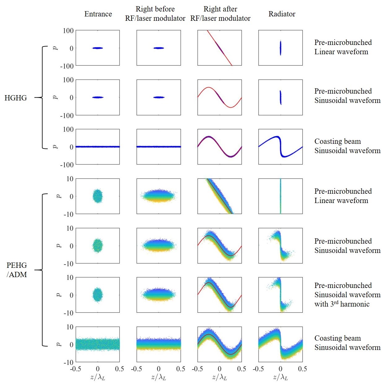
Figure 7: (Figure and caption from Ref. [25]) Application of HGHG and PEHG/ADM for bunch compression and harmonic generation. Parameters used in this example plot: $\lambda_{L}=1064$ nm, $\sigma_{zi}=30$ nm and $\sigma_{zf}=3$ nm for the case of a pre-microbunched beam, $\sigma_{\delta i}=3\times 10^{-4}$, $\sigma_{yi}=2\ \mu$m, $\sigma_{y^{\prime}i}=1\ \mu$rad. The figures show the beam distribution evolution in the longitudinal phase space. The different colors of the particles in the plots of PEHG/ADM correspond to different $y$ for PEHG or $y^{\prime}$ for ADM. The modulation waveforms are shown in the figure as the red curves. Note that the range of vertical axis $p=\delta/\sigma_{\delta i}$ in PEHG/ADM is one order of magnitude smaller than that of HGHG in this figure. In this figure, we have also shown the example of applying third laser harmonic to broaden the linear zone of the modulation waveform to enhance the final bunching factor.

5.2 Realization Examples

After doing the general mathematical analysis, here we introduce several concrete examples of the realization of this energy modulation-based coupling scheme. We remind the readers that the content of this section has been presented before in Ref. [25].

5.2.1 PEHG

The first proposal to apply energy modulation-based TLC as we defined for microbunching generation to our knowledge is phase-merging enhanced harmonic generation (PEHG) [22, 23], which is then followed by angular dispersion-induced microbunching (ADM) [24]. There are also other novel ideas being proposed [25]. Here we give a brief introduction of PEHG and ADM.

PEHG is first proposed for an efficient frequency up-conversion in FEL seeding [22, 23]. A PEHG unit can be divided into four key functional components: (i) a dispersion generation ($R_{36}=d$) device, for example, a dogleg, to correlate $y$ with $\delta$; (ii) a laser modulator to generate an energy chirp ($R_{65}=h$) to correlate $\delta$ with $z$; (iii) a dispersive section ($R_{56}$) for longitudinal phase-space shearing to correlate $z$ with $\delta$ to form microbunching; and (iv) a phase-merging unit ($R_{53}=D^{\prime}$) to correlate $z$ with $y$. The trick for phase merging is to achieve cancellation between the longitudinal displacement contribution from $\delta$ (through $R_{56}$) and that from $y$ introduced in the first step (through $dD^{\prime}$), thus causing the longitudinal phases of different particles to merge together. This process can be understood with the help of Fig 7.

Now we conduct a matrix analysis to present the physical principle of PEHG as explained above. By using matrix, it means that we have linearized the sine waveform around the zero-crossing phase. Therefore, here we actually treat PEHG as a bunch compression scheme as we defined in Sec. 4. The thin-lens transfer matrices of the four functions mentioned above are

$${\bf M}_{\text{1}}=\left(\begin{matrix}1&0&0&d\\ 0&1&0&0\\ 0&d&1&0\\ 0&0&0&1\\ \end{matrix}\right),\ {\bf M}_{\text{2}}=\left(\begin{matrix}1&0&0&0\\ 0&1&0&0\\ 0&0&1&0\\ 0&0&h&1\\ \end{matrix}\right),$$ (148)

$${\bf M}_{\text{3}}=\left(\begin{matrix}1&0&0&0\\ 0&1&0&0\\ 0&0&1&R_{56}\\ 0&0&0&1\\ \end{matrix}\right),\ {\bf M}_{\text{4}}=\left(\begin{matrix}1&0&0&0\\ 0&1&0&-D^{\prime}\\ D^{\prime}&0&1&0\\ 0&0&0&1\\ \end{matrix}\right),$$

where $h=k_{L}A$. Note that here we focus on the key matrix elements of each function, with only fundamental physical principle of symplecticity taken into account. With such simplification, the total transfer matrix of a PEHG unit is

$${\bf T}={\bf M}_{\text{4}}{\bf M}_{\text{3}}{\bf M}_{\text{2}}{\bf M}_{\text{1}}=\left(\begin{matrix}1&0&0&d\\ 0&1-dhD^{\prime}&-hD^{\prime}&-D^{\prime}\\ D^{\prime}&d\left(hR_{56}+1\right)&hR_{56}+1&dD^{\prime}+R_{56}\\ 0&hD^{\prime}&h&1\\ \end{matrix}\right).$$ (149)

To achieve optimal bunch compression, we need $hR_{56}+1=0$ and $dD^{\prime}+R_{56}=0$, then

$$\sigma_{zf}=|D^{\prime}|\sigma_{yi}=\bigg{|}\frac{R_{56}}{d}\bigg{|}\sigma_{yi},$$ (150)

where the subscripts _i and _f represent ‘initial’ and ‘final’, respectively. Note that $\sigma_{z}$ here means the microbunch length, and is different from the usual bunch length in an FEL which is much longer than the modulation laser wavelength. Therefore, the final bunch length in PEHG depends solely on the initial vertical beam size. As a comparison, in HGHG, $\sigma_{zf}=|R_{56}|\sigma_{\delta i}$. In correspondence to that of HGHG, the effective energy spread of PEHG is $\sigma_{\delta,\text{eff}}=\frac{\sigma_{yi}}{|d|}$. So PEHG is favorable for harmonic generation or bunch compression when $\frac{\sigma_{yi}}{|d|}<\sigma_{\delta i}$.

Considering that the modulation waveform is actually a nonlinear sine, and for a coasting beam, the final bunching factor at the $n^{\text{th}}$ laser harmonic in PEHG is [22, 23]

$$b_{n}=J_{n}(-nk_{L}A{R}_{56})\text{exp}\left[-{\left(nk_{L}D^{\prime}\sigma_{yi}\right)^{2}}/{2}\right],$$ (151)

where $A=\frac{h}{k_{L}}$. Note that considering the nonlinear sine modulation waveform, the optimal microbunching condition for a specific harmonic is slightly different from our simplified linear analysis, $1+hR_{56}=0$.

To better illustrate the mechanism, we have divided the PEHG process into four functions. Note that there is some flexibility in their order. Additionally, these functions can be realized one by one, or with two or three of them simultaneously. In the original publication on PEHG [22], a transverse-gradient undulator was applied along with the modulation laser to realize energy chirping and phase merging at the same time. There are PEHG variants proposed where a normal undulator is used and phase merging is realized elsewhere.

5.2.2 ADM

ADM is first proposed for efficient coherent harmonic generation in a storage ring FEL [24], by making use of the fact that the vertical emittance in a planar $x$-$y$ uncoupled ring is rather small. Different from PEHG, which uses the dispersion at the modulator, ADM invokes the dispersion angle, based on which the name angular dispersion-induced microbunching is coined. In the original publication [24], an ADM unit consists of (i) a dipole to generate the dispersion angle ($R_{46}=-d^{\prime}$); (ii) a laser modulator to energy modulate the electron beam ($R_{65}=h$); (iii) a dogleg to generate micorbunching ($R_{56}$ and $R_{54}=D$). Here we also conduct a matrix analysis of ADM like that for PEHG. The thin-lens transfer matrices of the three parts of an ADM unit are

$${\bf M}_{\text{1}}=\left(\begin{array}[]{cccc}1&0&0&0\\ 0&1&0&-d^{\prime}\\ d^{\prime}&0&1&0\\ 0&0&0&1\\ \end{array}\right),\ {\bf M}_{\text{2}}=\left(\begin{matrix}1&0&0&0\\ 0&1&0&0\\ 0&0&1&0\\ 0&0&h&1\\ \end{matrix}\right),\ {\bf M}_{\text{3}}=\left(\begin{array}[]{cccc}1&0&0&D\\ 0&1&0&0\\ 0&D&1&R_{56}\\ 0&0&0&1\\ \end{array}\right).$$ (152)

Then the total transfer matrix is

$${\bf T}={\bf M}_{\text{3}}{\bf M}_{\text{2}}{\bf M}_{\text{1}}=\left(\begin{array}[]{cccc}d^{\prime}hD+1&0&hD&D\\ 0&1&0&-d^{\prime}\\ d^{\prime}\left(hR_{56}+1\right)&D&hR_{56}+1&-d^{\prime}D+R_{56}\\ d^{\prime}h&0&h&1\\ \end{array}\right).$$ (153)

To achieve optimal bunch compression, we need $hR_{56}+1=0,\ -d^{\prime}D+R_{56}=0,$ then

$$\sigma_{zf}=|D|\sigma_{y^{\prime}i}=\bigg{|}\frac{R_{56}}{d^{\prime}}\bigg{|}\sigma_{y^{\prime}i}.$$ (154)

So the final bunch length depends solely on the initial vertical beam divergence. In correspondence to that of HGHG, the effective energy spread of ADM is $\sigma_{\delta,\text{eff}}=\frac{\sigma_{y^{\prime}i}}{|d^{\prime}|}$. Therefore, ADM is favorable compared to HGHG for harmonic generation or bunch compression when $\frac{\sigma_{y^{\prime}i}}{|d^{\prime}|}<\sigma_{\delta i}$. Considering the nonlinear sine modulation waveform, and for a coasting beam, the final bunching factor at the $n^{\text{th}}$ laser harmonic in ADM is [24]

$$b_{n}=J_{n}(-nk_{L}A{R}_{56})\text{exp}\left[-{\left(nk_{L}D\sigma_{y^{\prime}i}\right)^{2}}/{2}\right].$$ (155)

As can be seen from the above analysis, PEHG and ADM are specific examples of our general definition of TLC-based microbunching schemes in Theorem One.

5.3 Modulation Strength

Now we derive the formula of modulation strength, given the laser, electron and undulator parameters. This is a necessary work for quantitative analysis and comparison. The most common method of imprinting energy modulation on electron beam at laser wavelength is using a TEM00 mode laser to resonant with the electron in an undulator. Below we use a planar undulator as the modulator. A helical undulator can also be applied for energy modulation, but since we want to preserve the ultrasmall vertical emittance, we want to avoid $x$-$y$ coupling as much as possible, and thus planar undulator might be preferred.

5.3.1 A Normally Incident Laser

The electromagnetic field of a TEM00 mode Gaussian laser polarized in the horizontal plane is [26]

$$\left(\begin{matrix}E_{x}\\ E_{y}\\ E_{z}\\ cB_{x}\\ cB_{y}\\ cB_{z}\end{matrix}\right)=E_{x0}e^{ik_{L}z-i\omega_{L}t+i\phi_{0}}\left(-iZ_{R}Q\right)\text{exp}\left[i\frac{k_{L}Q}{2}\left(x^{2}+y^{2}\right)\right]\left(\begin{matrix}1\\ 0\\ -Qx\\ -Q^{2}xy\\ Q^{2}x^{2}-\frac{iQ}{k_{L}}+1\\ -Qy\end{matrix}\right),$$ (156)

with $\lambda_{L}$ the laser wavelength, $k_{L}=\frac{2\pi}{\lambda_{L}}$ the wavenumber of laser, $c$ the speed of light in free space and $\omega_{L}=k_{L}c$, $Z_{R}=\frac{\pi w_{0}^{2}}{\lambda_{L}}$ the Rayleigh length, $w_{0}$ the beam waist radius, and $Q=\frac{i}{Z_{R}(1+\frac{z}{Z_{R}})}$. We remind the readers that we have used $t$ to represent the angular chirp strength in previous and some of the later analysis, while here it means time. We hope their difference should be clear from the context. The relation between the peak electric field $E_{x0}$ and the laser peak power $P_{L}$ is given by

$$P_{L}=\frac{E_{x0}^{2}Z_{R}\lambda_{L}}{4Z_{0}},$$ (157)

in which $Z_{0}=376.73\ \Omega$ is the impedance of free space. The prescribed wiggling motion of electron in a planar undulator is

$$x(z)=\frac{K}{\gamma k_{u}}\sin(k_{u}z),$$ (158)

with $\gamma$ the Lorentz factor, $K=\frac{eB_{0}\lambda_{u}}{2\pi m_{e}c}=0.934\cdot B_{0}[\text{T}]\cdot\lambda_{u}[\text{cm}]$ the dimensionless undulator parameter, $B_{0}$ the peak magnetic field, $\lambda_{u}$ the undulator period, and $k_{u}=\frac{2\pi}{\lambda_{u}}$. The resonant condition of laser-electron interaction inside a planar undulator is

$$\lambda_{L}=\frac{1+\frac{K^{2}}{2}}{2\gamma^{2}}\lambda_{u}.$$ (159)

From the prescribed motion we can calculate the electron horizontal and longitudinal velocity

$$v_{x}(z) \approx\frac{\beta cK}{\gamma}\cos(k_{u}z),$$ (160)

$$v_{z}(z) =\sqrt{v^{2}-v_{x}^{2}}=\beta c\sqrt{1-\left[\frac{K}{\gamma}\cos(k_{u}z)\right]^{2}}$$

$$\approx c\left(1-\frac{1}{2\gamma^{2}}\right)\left[1-\frac{K^{2}/2}{2\gamma^{2}}\left(1+\cos(2k_{u}z)\right)\right]$$

$$\approx c\left(1-\frac{1+K^{2}/2}{2\gamma^{2}}\right)-\frac{cK^{2}}{4\gamma^{2}}\cos(2k_{u}z).$$

Therefore, we have

$$\bar{v}_{z} =c\left(1-\frac{1+K^{2}/2}{2\gamma^{2}}\right),$$ (161)

$$z(t) \approx\bar{v}_{z}t-\frac{K^{2}}{8\gamma^{2}k_{u}}\sin(2k_{u}\bar{v}_{z}t).$$

Then

$$k_{L}z-\omega_{L}t\approx\left(\bar{v}_{z}-c\right)k_{L}t-\frac{K^{2}k_{L}}{8\gamma^{2}k_{u}}\sin(2k_{u}\bar{v}_{z}t)\approx-k_{u}z-\chi\sin(2k_{u}z),$$ (162)

where $\chi=\frac{K^{2}k_{L}}{8\gamma^{2}k_{u}}=\frac{K^{2}}{4+2K^{2}}$. Note that since the longitudinal coordinate $z$ of electron will affect the laser phase observed, so we need to calculate its precision to the order of $\frac{1}{\gamma^{2}}$. While for the horizontal coordinate $x$, we only need to calculate it to the order of $\frac{1}{\gamma}$. In the following, we will adopt the approximation $\beta\approx 1$ since we are interested in relativistic cases.

Given the electron prescribed motion and laser electric field, the laser and electron exchange energy according to

$$\frac{dW}{dt}=ev_{x}E_{x}+ev_{z}E_{z}.$$ (163)

Assuming that the laser beam waist is in the middle of the undulator, whose length is $L_{u}$, and when $x,y\ll w(z)$, which is true in most of our interested cases, we drop the $\text{exp}\left[i\frac{k_{L}Q}{2}(x^{2}+y^{2})\right]$ in the laser electric field. Further, when $x\ll Z_{R}$ which is also satisfied in our interested cases, we can also drop the contribution from $E_{z}$ on the energy modulation. The integrated modulation voltage induced by the laser on the electron beam in a planar undulator is then

$$V_{L} \approx\text{Re}\left[\int_{-\frac{L_{u}}{2}}^{\frac{L_{u}}{2}}v_{x}E_{x}\frac{dz}{c}\right]$$ (164)

$$\approx\text{Re}\left[\int_{-\frac{L_{u}}{2}}^{\frac{L_{u}}{2}}E_{x0}e^{ik_{L}z-i\omega_{L}t+i\phi_{0}}\frac{1}{1+i\frac{z}{Z_{R}}}\frac{cK}{\gamma}\cos(k_{u}z)\frac{dz}{c}\right]$$

$$\approx E_{x0}\frac{K}{\gamma}\text{Re}\left[e^{i\phi_{0}}\int_{-\frac{L_{u}}{2}}^{\frac{L_{u}}{2}}e^{-ik_{u}z-i\chi\sin(2k_{u}z)}\frac{1}{1+i\frac{z}{Z_{R}}}\frac{e^{ik_{u}z}+e^{-ik_{u}z}}{2}dz\right]$$

$$=E_{x0}\frac{K}{\gamma}\text{Re}\left[e^{i\phi_{0}}\int_{-\frac{L_{u}}{2}}^{\frac{L_{u}}{2}}\frac{1}{1+i\frac{z}{Z_{R}}}\sum_{n=-\infty}^{\infty}J_{n}(-\chi)e^{in2k_{u}z}\frac{1+e^{-i2k_{u}z}}{2}dz\right],$$

where Re() means taking the real component of the complex number. When $L_{u}\gg\lambda_{u}$, which means the undulator period number $N_{u}\gg 1$, in the above integration, only the term with $n=0$ and $n=1$ will give notable non-vanishing value. Denote $[JJ]\equiv J_{0}(\chi)-J_{1}(\chi)$, we then have

$$V_{L} =E_{x0}\frac{K}{\gamma}\frac{[JJ]}{2}\text{Re}\left[e^{i\phi_{0}}\int_{-\frac{L_{u}}{2}}^{\frac{L_{u}}{2}}\frac{1-i\frac{z}{Z_{R}}}{1+\left(\frac{z}{Z_{R}}\right)^{2}}dz\right]$$ (165)

$$=E_{x0}\frac{K}{\gamma}[JJ]Z_{R}\tan^{-1}\left(\frac{L_{u}}{2Z_{R}}\right)\cos\phi_{0}.$$

We want the energy modulation strength as large as possible, so we choose $\phi_{0}=0$. Put in the expression of peak electric field from Eq. (157), we have

$$V_{L} =\frac{K[JJ]}{\gamma}\sqrt{\frac{4P_{L}Z_{0}Z_{R}}{\lambda_{L}}}\tan^{-1}\left(\frac{L_{u}}{2Z_{R}}\right).$$ (166)

The above result has also been obtained before in Ref. [26]. The linear energy chirp strength around the zero-crossing phase is therefore

$$h=\frac{eV_{L}}{E_{0}}k_{L}=\frac{ek_{L}K[JJ]}{\gamma^{2}m_{e}c^{2}}\sqrt{\frac{2P_{L}Z_{0}}{\lambda_{L}}}\frac{\tan^{-1}\left(\frac{L_{u}}{2Z_{R}}\right)}{\sqrt{\frac{L_{u}}{2Z_{R}}}}\sqrt{L_{u}},$$ (167)

where $E_{0}$ is the electron energy and $m_{e}$ is the mass of electron. Once the modulator length is given, we can optimize the laser Rayleigh length to maximize the energy modulation. Figure 8 below is a plot of $f(x)=\frac{\tan^{-1}(x)}{\sqrt{x}}$ as a function of $x$. The maximum value of $f(x)$ is 0.8034 and is realized when $x=1.392$. So when $Z_{R}=\frac{L_{u}}{2\times 1.392}=0.359L_{u}$, the energy modulation reaches the maximum value. Note that when $Z_{R}$ is within a small range close to the optimal value, the impact of Rayleight length change on energy modulation strength is not very sensitive. Therefore, for easy of remembering, the optimal condition can be expressed as $Z_{R}\approx\frac{L_{u}}{3}$. From Eq. (167), we can see that given $\frac{L_{u}}{2Z_{R}}$, we have $h\propto\sqrt{P_{L}}$ and $h\propto\sqrt{L_{u}}$.

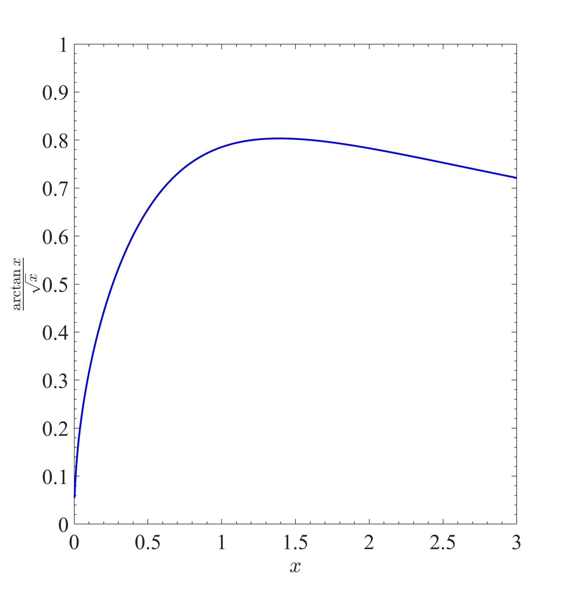
Figure 8: $f(x)=\frac{\tan^{-1}(x)}{\sqrt{x}}$ v.s. $x$.

From Eq. (167) we can do some example calculation to get a more concrete feeling. If $E_{0}=600$ MeV, $\lambda_{L}=1064$ nm, $\lambda_{u}=8$ cm ($B_{0}=1.13$ T), $L_{u}=0.8$ m ($N_{u}=10$), $Z_{R}=0.359L_{u}$, then the induced energy chirp strength with $P_{L}=1$ MW is $h=955\ \text{m}^{-1}$.

5.3.2 Dual-Tilted-Laser for Energy Modulation

Now with a hope to increase the energy modulation strength with a given laser power, we may use a configuration of crossing two lasers for energy modulation. The basic idea is that if two crossing lasers can double the energy modulation strength of that of a single laser, then the effect is like that induced by single laser with a laser power four times larger. Our calculation shows that indeed dual-tilted-laser (DTL) can induce a larger energy modulation compared to that of a single laser, but the issue is that the required crossing angle is too small (1 mrad level) from an engineering viewpoint.

Now we present the analysis. First we consider the case of two lasers crossing in the $y$-$z$ plane. The laser field of an oblique TEM00 laser is given by first replacing the physical coordinate with the rotated coordinates

$$x\rightarrow x,\ y\rightarrow y_{1}=y\cos\theta+z\sin\theta,\ z\rightarrow z_{1}=-y\sin\theta+z\cos\theta,\ t\rightarrow t,$$ (168)

and the result according to Eq. (156) is

$$\left(\begin{matrix}E_{x}\\ E_{y}\\ E_{z}\\ cB_{x}\\ cB_{y}\\ cB_{z}\end{matrix}\right)_{\text{rot}}=E_{x0}e^{ik_{L}z_{1}-i\omega_{L}t}\frac{\text{exp}\left[-\frac{k_{L}(x^{2}+y_{1}^{2})}{2(Z_{R}+iz_{1})}\right]}{1+i\frac{z_{1}}{Z_{R}}}\left(\begin{matrix}1\\ 0\\ -i\frac{x}{Z_{R}+iz_{1}}\\ \frac{xy_{1}}{\left(Z_{R}+iz_{1}\right)^{2}}\\ -\frac{x^{2}}{\left(Z_{R}+iz_{1}\right)^{2}}-\frac{1}{k_{L}\left(Z_{R}+iz_{1}\right)}+1\\ -i\frac{y_{1}}{Z_{R}+iz_{1}}\end{matrix}\right).$$ (169)

But note that in the above expression $x,y,z$ of the electromagnetic fields are the direction defined according to the oblique laser propagating direction. To get the expression back in the original coordinate system, i.e., undulator axis as the $z$ axis, we need to rotate the laser field again,

$$E_{x}\rightarrow E_{x\text{rot}},\ E_{y}\rightarrow E_{y}=E_{y\text{rot}}\cos\theta-E_{z\text{rot}}\sin\theta,\ E_{z}\rightarrow E_{z}=E_{y\text{rot}}\sin\theta+E_{z\text{rot}}\cos\theta,\ t\rightarrow t,$$ (170)

and for the electric field the result is

$$\left(\begin{matrix}E_{x}\\ E_{y}\\ E_{z}\\ \end{matrix}\right)_{\text{unrot}}=E_{x0}e^{ik_{L}z_{1}-i\omega_{L}t}\frac{\text{exp}\left[-\frac{k_{L}(x^{2}+y_{1}^{2})}{2(Z_{R}+iz_{1})}\right]}{1+i\frac{z_{1}}{Z_{R}}}\left(\begin{matrix}1\\ -i\frac{x}{Z_{R}+iz_{1}}\sin\theta\\ -i\frac{x}{Z_{R}+iz_{1}}\cos\theta\\ \end{matrix}\right).$$ (171)

Assuming that the two crossing lasers are in-phase and have the same amplitude. In addition, we assume that $\theta_{2}=-\theta_{1}=-\theta$, and the two lasers have the same Rayleigh lengths. Then the superimposed field is

$$\left(\begin{matrix}E_{x}\\ E_{y}\\ E_{z}\\ \end{matrix}\right)_{\text{unrot}}=$$ (172)

$$E_{x0}e^{ik_{L}\left(-y\sin\theta+z\cos\theta\right)-i\omega_{L}t}\frac{\text{exp}\left[-\frac{k_{L}(x^{2}+\left(y\cos\theta+z\sin\theta\right)^{2})}{2(Z_{R}+i\left(-y\sin\theta+z\cos\theta\right))}\right]}{1+i\frac{\left(-y\sin\theta+z\cos\theta\right)}{Z_{R}}}\left(\begin{matrix}1\\ -i\frac{x}{Z_{R}+i\left(-y\sin\theta+z\cos\theta\right)}\sin\theta\\ -i\frac{x}{Z_{R}+i\left(-y\sin\theta+z\cos\theta\right)}\cos\theta\\ \end{matrix}\right)$$

$$+E_{x0}e^{ik_{L}\left(y\sin\theta+z\cos\theta\right)-i\omega_{L}t}\frac{\text{exp}\left[-\frac{k_{L}(x^{2}+\left(y\cos\theta-z\sin\theta\right)^{2})}{2(Z_{R}+i\left(y\sin\theta+z\cos\theta\right))}\right]}{1+i\frac{\left(y\sin\theta+z\cos\theta\right)}{Z_{R}}}\left(\begin{matrix}1\\ i\frac{x}{Z_{R}+i\left(y\sin\theta+z\cos\theta\right)}\sin\theta\\ -i\frac{x}{Z_{R}+i\left(y\sin\theta+z\cos\theta\right)}\cos\theta\\ \end{matrix}\right).$$

As before here we focus on the impact of $E_{x}$ on laser-electron interaction, and ignore the contribution from $E_{z}$. When $\theta$ is very small, $E_{x}$ can be approximated as

$$E_{x} =2E_{x0}\frac{\exp\left[ik_{L}z\cos\theta-i\omega t-\frac{k_{L}\left(x^{2}+z^{2}\sin^{2}\theta\right)}{2\left(Z_{R}+iz\cos\theta\right)}\right]}{1+\frac{iz\cos\theta}{Z_{R}}}$$ (173)

$$\approx 2E_{x0}e^{ik_{L}z\cos\theta-i\omega_{L}t}\frac{\exp\left[-\frac{k_{L}z^{2}\theta^{2}}{2\left(Z_{R}+iz\right)}\right]}{1+i\frac{z}{Z_{R}}}.$$

Note that in the final approximated expression, we have kept $z\cos\theta$ in the laser phase term. The reason is that the laser phase is of key importance in laser-electron interaction and the accuracy requirement is high. In addition, we have also kept the $z^{2}\theta^{2}$ in the intensity decay term, this is because $L_{u}\theta$ may not be small compared to the laser beam wait size $w_{0}$. The expression of $E_{x}$ for the case of crossing in $x$-$z$ plane is similar. So the difference of crossing in $x$-$z$ plane and $y$-$z$ plane is not much in inducing energy modulation.

For effective laser-electron interaction, the off-axis resonance condition now is

$$c\frac{\lambda_{u}}{\bar{v}_{z}}-\lambda_{u}\cos\theta=\lambda_{L},$$ (174)

or

$$\lambda_{L}=\left(\frac{1}{1-\frac{1+\frac{K^{2}}{2}}{2\gamma^{2}}}-\cos\theta\right)\lambda_{u}\approx\frac{1+\frac{K^{2}}{2}+\gamma^{2}\theta^{2}}{2\gamma^{2}}\lambda_{u}.$$ (175)

Then

$$k_{L}z-\omega_{L}t\approx\left(\bar{v}_{z}-c\right)k_{L}t-\frac{K^{2}k_{L}}{8\gamma^{2}k_{u}}\sin(2k_{u}\bar{v}_{z}t)\approx-k_{u}z-\chi\sin(2k_{u}z).$$ (176)

Note that now $\chi$ depends on $\theta$, more specifically,

$$\chi=\frac{K^{2}k_{L}}{8\gamma^{2}k_{u}}\approx\frac{K^{2}}{4+2K^{2}+4\gamma^{2}\theta^{2}}.$$ (177)

Denote $v\equiv\frac{k_{L}Z_{R}\theta^{2}}{2}=\left(\frac{Z_{R}\theta}{w_{0}}\right)^{2}$. Assume that the laser beam waists are in the middle of undulator, whose length is $L_{u}$, the integrated modulation voltage induced by the DTL in a planar undulator is then

$$V_{L} \approx\text{Re}\left[\int_{-\frac{L_{u}}{2}}^{\frac{L_{u}}{2}}v_{x}E_{x}\frac{dz}{c}\right]$$ (178)

$$\approx\text{Re}\left[\int_{-\frac{L_{u}}{2}}^{\frac{L_{u}}{2}}2E_{x0}e^{ik_{L}z\cos\theta-i\omega_{L}t+i\phi_{0}}\frac{\exp\left[-\frac{k_{L}z^{2}\theta^{2}}{2\left(Z_{R}+iz\right)}\right]}{1+i\frac{z}{Z_{R}}}\frac{cK}{\gamma}\cos(k_{u}z)\frac{dz}{c}\right]$$

$$\approx 2E_{x0}\frac{K}{\gamma}\text{Re}\left[e^{i\phi_{0}}\int_{-\frac{L_{u}}{2}}^{\frac{L_{u}}{2}}e^{-ik_{u}z-i\chi\sin(2k_{u}z)}\frac{\exp\left[-\frac{z^{2}\theta^{2}}{w_{0}^{2}\left(1+i\frac{z}{Z_{R}}\right)}\right]}{1+i\frac{z}{Z_{R}}}\frac{e^{ik_{u}z}+e^{-ik_{u}z}}{2}dz\right]$$

$$\approx E_{x0}\frac{K[JJ]}{\gamma}\text{Re}\left[e^{i\phi_{0}}\int_{-\frac{L_{u}}{2}}^{\frac{L_{u}}{2}}\frac{\exp\left[-\frac{z^{2}\theta^{2}}{w_{0}^{2}\left(1+i\frac{z}{Z_{R}}\right)}\right]}{1+i\frac{z}{Z_{R}}}dz\right]$$

$$\approx E_{x0}\frac{K[JJ]}{\gamma}Z_{R}\text{Re}\left[e^{i\phi_{0}}\int_{-\frac{L_{u}}{2Z_{R}}}^{\frac{L_{u}}{2Z_{R}}}\frac{\exp\left(-\frac{Z_{R}^{2}\theta^{2}{u}^{2}}{w_{0}^{2}\left(1+i{u}\right)}\right)}{1+i{u}}d{u}\right]$$

$$=E_{x0}\frac{K[JJ]}{\gamma}Z_{R}\text{Re}\left[e^{i\phi_{0}}\int_{-\frac{L_{u}}{2Z_{R}}}^{\frac{L_{u}}{2Z_{R}}}\frac{\exp\left(-v\frac{{u}^{2}}{1+{u}^{2}}\right)}{1+{u}^{2}}\left[\cos\left(v\frac{{u}^{3}}{1+{u}^{2}}\right)+{u}\sin\left(v\frac{{u}^{3}}{1+{u}^{2}}\right)\right.\right.$$

$$\left.\left.\ \ \ \ \ \ \ \ +i\left(\sin\left(v\frac{{u}^{3}}{1+{u}^{2}}\right)-{u}\cos\left(v\frac{{u}^{3}}{1+{u}^{2}}\right)\right)\right]d{u}\right]$$

$$=E_{x0}\frac{K[JJ]}{\gamma}Z_{R}\int_{-\frac{L_{u}}{2Z_{R}}}^{\frac{L_{u}}{2Z_{R}}}\frac{\exp\left(-v\frac{{u}^{2}}{1+{u}^{2}}\right)}{1+{u}^{2}}\left[\cos\left(v\frac{{u}^{3}}{1+{u}^{2}}\right)+{u}\sin\left(v\frac{{u}^{3}}{1+{u}^{2}}\right)\right]d{u}\cos\phi_{0}.$$

To maximize the energy modulation, we choose $\phi_{0}=0$. Then

$$V_{L}=E_{x0}\frac{K[JJ]}{\gamma}Z_{R}\int_{-\frac{L_{u}}{2Z_{R}}}^{\frac{L_{u}}{2Z_{R}}}\frac{\exp\left(-v\frac{{u}^{2}}{1+{u}^{2}}\right)}{1+{u}^{2}}\left[\cos\left(v\frac{{u}^{3}}{1+{u}^{2}}\right)+{u}\sin\left(v\frac{{u}^{3}}{1+{u}^{2}}\right)\right]d{u}.$$ (179)

Put in the expression of $E_{x0}$ from Eq. (157), the linear energy chirp strength around the zero-crossing phase is therefore

$$h=\frac{eV_{L}}{E_{0}}k_{L}=\frac{ek_{L}K[JJ]}{\gamma^{2}m_{e}c^{2}}\sqrt{\frac{2P_{L}Z_{0}}{\lambda_{L}}}F_{\text{DTL-E}}\left(\frac{L_{u}}{2Z_{R}},\frac{k_{L}Z_{R}\theta^{2}}{2}\right)\sqrt{L_{u}},$$ (180)

where

$$F_{\text{DTL-E}}(x,v)=\frac{1}{\sqrt{x}}\int_{-x}^{x}\frac{\exp\left(-v\frac{{u}^{2}}{1+{u}^{2}}\right)}{1+{u}^{2}}\left[\cos\left(v\frac{{u}^{3}}{1+{u}^{2}}\right)+{u}\sin\left(v\frac{{u}^{3}}{1+{u}^{2}}\right)\right]d{u}.$$ (181)

A flat contour plot of $F_{\text{DTL-E}}(x,v)$ is given in Fig. 9.

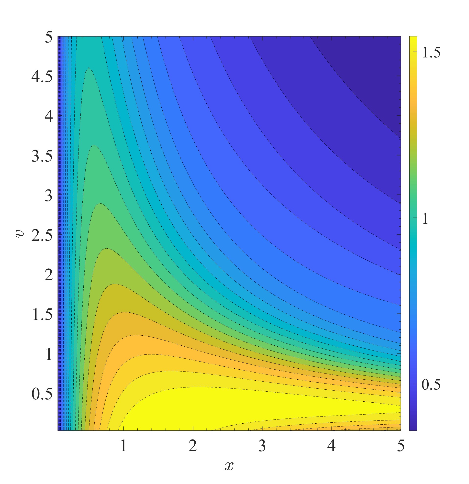
Figure 9: Contour plot of $F_{\text{DTL-E}}(x,v)$ given by Eq. (181).

Now we can use the derived formula to calculate the energy chirp strength induced by DTL. First we consider the case of keeping $\lambda_{u}$ fixed when changing $\theta$. If we keep $\lambda_{u}$ fixed when changing $\theta$, then the off-axis resonant condition can be expressed as

$$K_{\theta}=\sqrt{2}\sqrt{2\gamma^{2}\left(1-\frac{1}{\frac{\lambda_{L}}{\lambda_{u}}+\cos\theta}\right)-1}.$$ (182)

With the increase of $\theta$, $K_{\theta}$ will decrease. Note that $K_{\theta}\propto B_{0\theta}$, so $B_{0\theta}$ also decreases with the increase of $\theta$. An example calculation of $K_{\theta}$ v.s. $\theta$ is given in Fig. 10. And the corresponding contour plot of the energy chirp strength normalized by the largest energy chirp induced by a single normally incident laser, v.s. $\theta$ and $Z_{R}/L_{u}$, is given in Fig. 11.

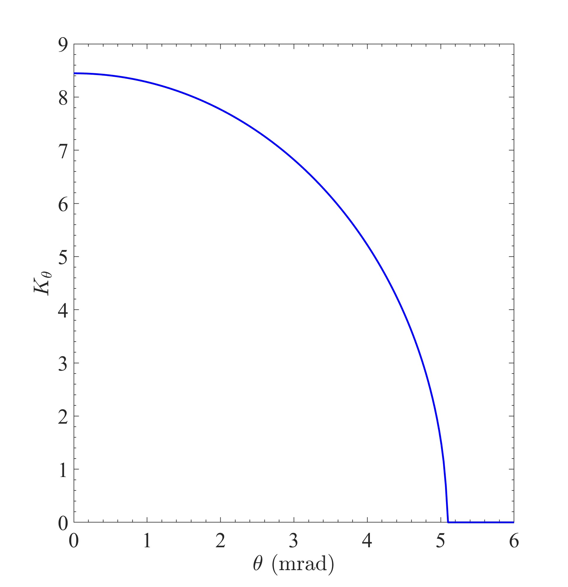
Figure 10: Undulator parameter $K_{\theta}$ v.s. $\theta$ with $\lambda_{u}$ kept fixed. Parameters used: $E_{0}=600$ MeV, $\lambda_{L}=1064$ nm, $\lambda_{u}=8$ cm.

Figure 11: Energy chirp strength $h$ normalized by the largest energy chirp induced by a single normally incident laser, v.s. $\theta$ and $Z_{R}/L_{u}$. Keep $\lambda_{u}$ fixed when changing $\theta$. Parameters used: $E_{0}=600$ MeV, $\lambda_{L}=1064$ nm, $\lambda_{u}=0.08$ m, $N_{u}=10$, $L_{u}=0.8$ m.

The previous calculation assumes $\lambda_{u}$ is kept unchanged when we adjust the incident angle $\theta$. This will result in a limited region of $\theta$ to fulfill resonant condition as shown in Fig. 10. Now we conduct the calculation by assuming the peak magnetic field $B_{0}$ unchanged when we adjust $\theta$. The off-axis resonant condition is

$$\lambda_{L}=\frac{1+\frac{K_{\theta}^{2}}{2}+\gamma^{2}\theta^{2}}{2\gamma^{2}}\lambda_{u},$$ (183)

where $K=\frac{eB_{0}}{2\pi m_{e}c}\lambda_{u}$, then

$$\frac{1}{2}\left(\frac{eB_{0}}{2\pi m_{e}c}\right)^{2}\lambda_{u}^{3}+(1+\gamma^{2}\theta^{2})\lambda_{u}-2\gamma^{2}\lambda_{L}=0,$$ (184)

from which we get

$$\lambda_{u}= \frac{2\pi^{2/3}\sqrt[3]{\sqrt{3}\sqrt{B_{0}^{6}c^{4}e^{6}m_{e}^{4}\left(27B_{0}^{2}\gamma^{4}e^{2}\lambda_{L}^{2}+8\pi^{2}c^{2}\left(\gamma^{2}\theta^{2}+1\right)^{3}m_{e}^{2}\right)}+9B_{0}^{4}c^{2}\gamma^{2}e^{4}m_{e}^{2}\lambda_{L}}}{3^{2/3}B_{0}^{2}e^{2}}$$ (185)

$$-\frac{4\pi^{4/3}c^{2}\left(\gamma^{2}\theta^{2}+1\right)m_{e}^{2}}{\sqrt[3]{3}\sqrt[3]{\sqrt{3}\sqrt{B_{0}^{6}c^{4}e^{6}m_{e}^{4}\left(27B_{0}^{2}\gamma^{4}e^{2}\lambda_{L}^{2}+8\pi^{2}c^{2}\left(\gamma^{2}\theta^{2}+1\right)^{3}m_{e}^{2}\right)}+9B_{0}^{4}c^{2}\gamma^{2}e^{4}m_{e}^{2}\lambda_{L}}}.$$

For example, if $\lambda_{L}=1064$ nm, $B_{0}=1.2$ T, then $\lambda_{u}$ as a function of $\theta$ for the case of $E_{0}=600$ MeV is shown in Fig. 12. Note that in this case $K_{\theta}\propto\lambda_{u\theta}$, so the undulator parameter also decreases with the increase of $\theta$. But the decrease is not that fast compared to that presented in Fig. 10. And the corresponding contour plot of the energy chirp strength induced by DTL normalized by the largest energy chirp induced by a single normally incident laser, v.s. $\theta$ and $Z_{R}/L_{u}$, is given in Fig. 13.

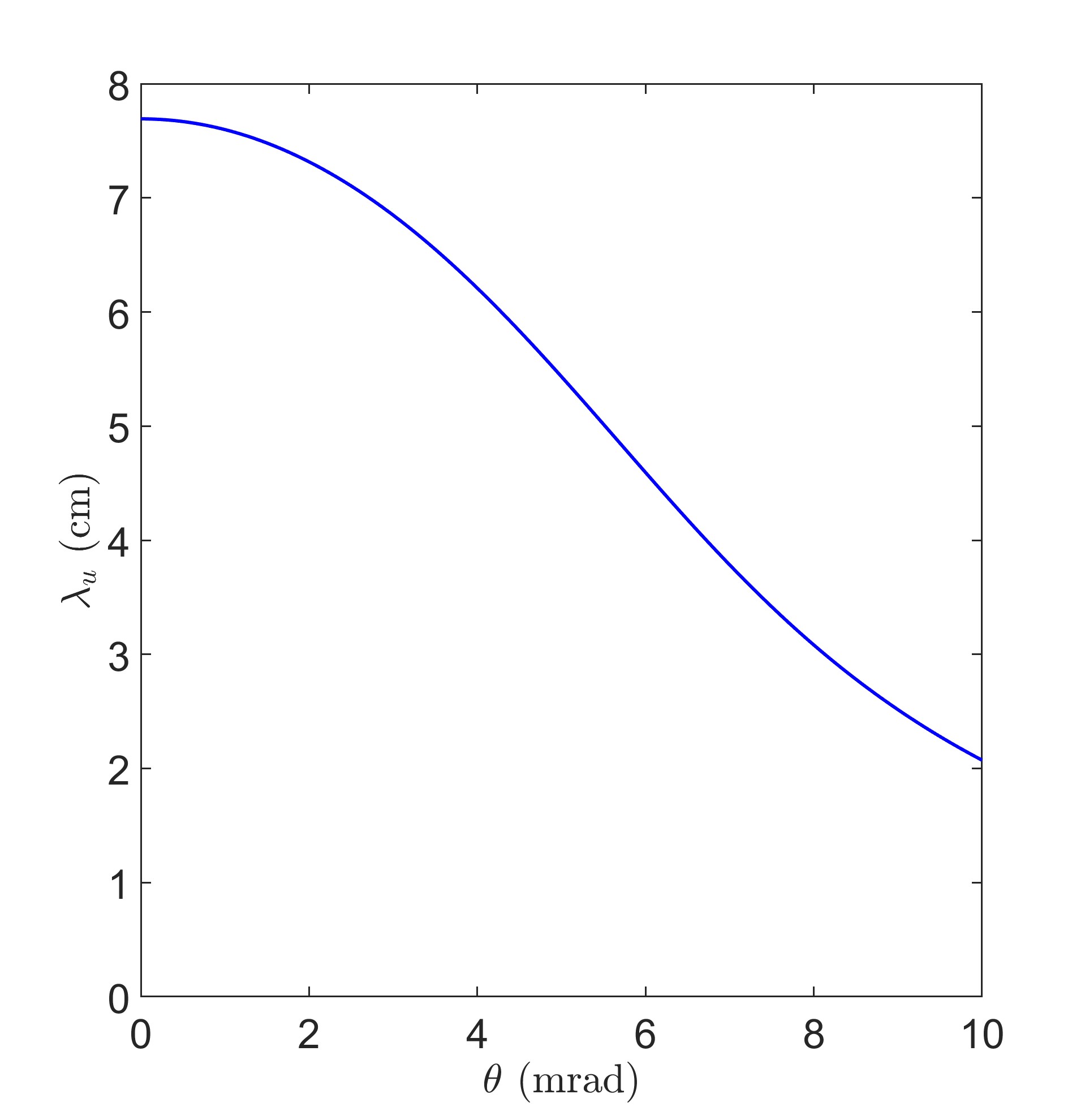
Figure 12: $\lambda_{u}$ v.s. $\theta$, with $B_{0}$ kept fixed. Parameters used: $E_{0}=600$ MeV, $\lambda_{L}=1064$ nm, $B_{0}=1.2$ T.

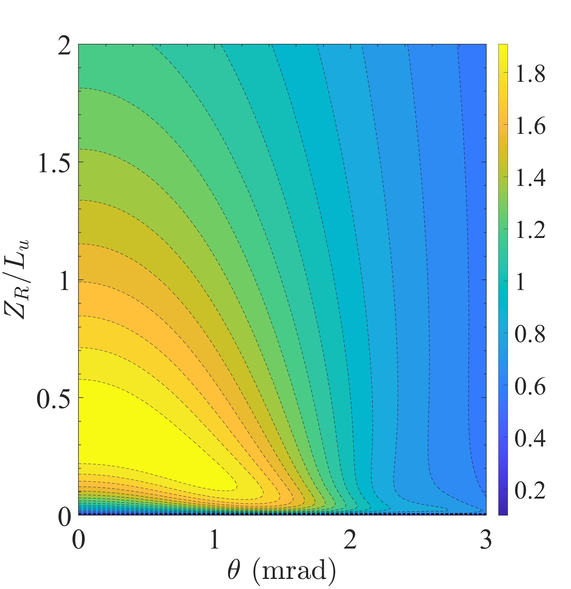
Figure 13: Energy chirp strength $h$ normalized by the largest energy chirp induced by a single normally incident laser, v.s. $\theta$ and $Z_{R}/L_{u}$. Keep $B_{0}$ fixed when changing $\theta$. Parameters used: $E_{0}=600$ MeV, $\lambda_{L}=1064$ nm, $B_{0}=1.2$ T, $L_{u}=0.8$ m.

As can be seen from the calculation results, Figs. 11 and 13, DTL indeed can induce a larger energy modulation compared to a single normally incident laser. But they required crossing angle (2 mrad level) is too small for engineering. So the usual setup of a single normally incident TEM00 mode laser is still the preferred choice in practical application.

6 Angular Modulation-Based Coupling Schemes

6.1 Bunching Factor

After investigating energy modulation-based TLC microbunching schemes, now in this section we discuss angular modulation-based ones. The problem definition is similar to that in the energy modulation-based schemes, only replacing the energy modulation by angular modulation. We use $y^{\prime}$ modulation as an example, since we will take advantage of the ultrasmall vertical emittance in a planar ring as explained before. The lumped laser-induced angular modulation is modeled as:

$$y^{\prime} =y^{\prime}+A\sin(k_{L}z),$$ (186)

$$\delta =\delta+Ak_{L}y\cos(k_{L}z).$$

Note that the above angular modulation is symplectic. Such an angular modulation process also satisfies the Panofsky-Wenzel theorem

$$\frac{\partial\Delta y^{\prime}}{\partial z}=\frac{\partial\Delta\delta}{\partial y}.$$ (187)

Following the bunching factor derivation in the section of energy modulation-based schemes, the generalized bunching factor at wavenumber $k$ in this case is

$$b(k) =\int\rho_{f}({\bf X})e^{-ik{\bf W}{\bf X}}d{\bf X}$$ (188)

$$=\int\rho_{m+}({\bf X})e^{-ik{\bf WR}{\bf X}}d{\bf X}$$

$$=\int\rho_{0}({\bf X})e^{-ik\left({\bf WR}{\bf X}+{\bf W}{\bf R}_{i4}A\sin(k_{L}z)+{\bf W}{\bf R}_{i6}Ak_{L}y\cos(k_{L}z)\right)}d{\bf X}$$

$$=\sum_{p_{1}=-\infty}^{\infty}J_{p_{1}}\left(-k{\bf W}{\bf R}_{i4}A\right)\int\rho_{0}({\bf X})\sum_{p_{2}=-\infty}^{\infty}i^{p_{2}}J_{p_{2}}\left(-k{\bf W}{\bf R}_{i6}Ak_{L}y\right)e^{-ik\left({\bf WR}{\bf X}-\frac{(p_{1}+p_{2})k_{L}}{k}z\right)}d{\bf X}.$$

The integration of the above result is given by generalized hypergeometric function.

To appreciate the physical principle, instead of a general mathematical analysis, we use one specific case as an example. If ${\bf W}=\left(\begin{matrix}0&0&0&0&1&0\end{matrix}\right)$ and $R_{56}=0$, then ${\bf W}{\bf R}_{i6}=0$, and

$$b(k) =\sum_{p=-\infty}^{\infty}J_{p}\left(-kR_{54}A\right)\text{exp}\left(-\frac{k^{2}}{2}{\bf M}_{\frac{pk_{L}}{k}}{\bf\Sigma}_{0}{\bf M}_{\frac{pk_{L}}{k}}^{T}\right).$$ (189)

If further $R_{51}=0$, $R_{52}=0$, and $R_{55}=1$, and the initial beam is transverse-longitudinal decoupled and has an upright distribution in the longitudinal phase space, then

$$b(k) =\sum_{p=-\infty}^{\infty}J_{p}\left(-kR_{54}A\right)\text{exp}\left(-\frac{k^{2}}{2}\left[\epsilon_{y}\left(R_{53}^{2}\beta_{y}-2R_{53}R_{54}\alpha_{y}+R_{54}^{2}{\gamma_{y}}\right)+\left(1-\frac{pk_{L}}{k}\right)^{2}\sigma_{z0}^{2}\right]\right).$$ (190)

If the initial bunch length is much longer than the laser wavelength, the above exponential terms will be non-zero only when $1-\frac{pk_{L}}{k}=0$, which means there is only bunching at the laser harmonics. In this case, we have the bunching factor at the $n$-th laser harmonic to be

$$b_{n}=b(nk_{L}) =J_{n}(-nk_{L}{R}_{54}A)\text{exp}\left[-\frac{\left(nk_{L}\right)^{2}}{2}\epsilon_{y}\mathcal{H}_{y\text{R}}\right],$$ (191)

where $\mathcal{H}_{y\text{R}}=R_{53}^{2}\beta_{y}-2R_{53}R_{54}\alpha_{y}+R_{54}^{2}{\gamma_{y}}$. One can appreciate the similarity of the above result with the bunching factor of energy modulation-based TLC microbunching schemes, i.e., Eq. (146). The $R_{54}$ here plays the role of $R_{56}$ there. If further $R_{53}=0$, then Eq. (191) reduces to

$$b_{n} =J_{n}(-nk_{L}{R}_{54}A)\text{exp}\left[-\frac{\left(nk_{L}R_{54}\sigma_{y^{\prime}}\right)^{2}}{2}\right],$$ (192)

where $\sigma_{y^{\prime}}$ is the initial beam angular divergence. So $R_{54}$ and $\sigma_{y^{\prime}}$ in this scheme play the role of $R_{56}$ and $\sigma_{\delta}$ in HGHG as shown in Eq. (134), respectively. In a planar uncoupled ring, the natural vertical emittance is quite small, thus also $\sigma_{y^{\prime}}$. Therefore, using this scheme we can realize a much higher harmonic bunching, without much impact on FEL lasing, compared to HGHG. This is the idea behind the proposal of Ref. [27].

As can be seen from our analysis, both the energy modulation-based and the angular modulation-based TLC microbunching schemes share the same spirit, i.e., to take advantage of the small transverse emittance, the vertical emittance in our case, to boost bunching. These TLC-based microbunching schemes can be viewed as partial transverse-longitudinal emittance exchange at the optical laser wavelength range. They do not necessarily need to be a complete emittance exchange since for microbunching, the most important coordinate is $z$, and $\delta$ is relatively less important. As we will show soon, although the spirit is the same, given the same level of modulation laser power, the physical realization of energy modulation-based TLC microbunching schemes turn out to be more effective for our SSMB application compared to angular modulation-based schemes.

6.2 Realization Examples and Modulation Strengths

The first proposal of applying the angular modulated beam for harmonic generation to our knowledge is from Ref. [27]. Later an emittance exchange-based harmonic generation scheme is proposed in Ref. [28]. These two schemes apply the TEM01 mode laser to induce angular modulation. Following these development, there is a proposal to realize angular modulation using a tilted incident TEM00 mode laser reported in Ref. [29]. And later a dual-tilted-laser (DTL) modulation scheme is applied in emittance exchange at the optical laser wavelength range[30]. And most recently, the DTL scheme is proposed to compress the bunch length in SSMB and lower the requiremnt on laser power by a factor of four compared to a single-tilted laser scheme[31]. Note that for these angular modulation based harmonic or bunch compression schemes, we have the inequality given in Eq. (95), i.e., our Theorem Two

$$t^{2}\beta_{y\text{M}}\mathcal{H}_{y\text{R}}\geq 1.$$ (193)

It might be helpful to make a short discussion on the relation between our angular modulation-based TLC analysis and the transverse-longitudinal emittance exchange (EEX). From the problem definition, for $\sigma_{z\text{R}}$ to be independent of $\epsilon_{z}$, we need

$$T_{55} =tR_{54}+1=0,$$ (194)

$$T_{56} =dR_{53}+d^{\prime}R_{54}+r_{56}\left(tR_{54}+1\right)+(dt+1)R_{56}=0.$$

From the problem definition in Sec. 4.1, for a complete EEX, we need the transfer matrix in the $y$-$z$ 4D phase space of the form

$${\bf T}=\left(\begin{matrix}{\bf 0}&{\bf F}\\ {\bf H}&{\bf 0}\end{matrix}\right).$$ (195)

Therefore, EEX is a special case in the context of our problem definition of TLC-based bunch compression, i.e., the final beam is then also $y$-$z$ decoupled. All we need is to add another condition to Eq. (194), i.e.,

$$dt+1=0.$$ (196)

After some straightforward algebra, the relations in Eqs. (194) and (196) can be summarized in an elegant form

$$t =-\frac{1}{d},$$ (197)

$$D =R_{34}d^{\prime}+R_{33}d,$$

$$D^{\prime} =R_{44}d^{\prime}+R_{43}d.$$

We remind the readers that energy modulation-based coupling schemes cannot accomplish complete transverse-longitudinal emittance exchange, since the matrix ${\bf I}$ in Eq. (100) cannot be ${\bf 0}$. Note also that to realize complete EEX, the angular modulator should be placed at a dispersive location, i.e., $d\neq 0$. However, for bunch compression purpose alone, the modulator can in principle be placed at a dispersion-free location. For example, to minimize the quantum excitation contribution of modulators to $\epsilon_{y}$, we may choose to place the modulator at a dispersion-free location, which means $d=0$ and $d^{\prime}=0$, then the bunch compression condition is

$$T_{55} =tR_{54}+1=0,$$ (198)

$$T_{56} =R_{56}=0.$$

To apply the TLC-based bunch compression scheme in GLSF SSMB, as explained most likely we need a reverse modulation section after the radiator where microbunching is formed and coherent radiation is generated, as shown in the schematic layout of GLSF SSMB in Fig. 4. Then in the above case, to do the reverse modulation, we need a downstream lattice which also has $R_{56}=0$ and in the meanwhile compensate the upstream $R_{54}$ and also $R_{53}$, such that the whole section between the two modulators (modulation + reverse modulation) is an isochronous achromat, and therefore the two modulations can cancel each other perfectly.

We remind the readers that the above discussion has been presented before in Refs. [8] and [25].

6.2.1 TEM01 Mode Laser-Induced Angular Modulation

The proposal in Ref. [27] is using a TEM01 mode laser to induce angular modulation on electron beam in an undulator. The electric field of a Hermite-Gaussian TEM01 mode laser polarized in the horizontal plane is [26]

$$\left(\begin{matrix}E_{x}\\ E_{y}\\ E_{z}\\ cB_{x}\\ cB_{y}\\ cB_{z}\end{matrix}\right)=E_{x0}e^{ik_{L}z-i\omega_{L}t}\left(-iZ_{R}Q\right)^{2}\text{exp}\left[i\frac{k_{L}Q}{2}\left(x^{2}+y^{2}\right)\right]\left(\frac{2\sqrt{2}}{w_{0}}\right)\left(\begin{matrix}y\\ 0\\ -Qxy\\ i\frac{Qx}{k_{L}}-Q^{2}xy^{2}\\ \left(Q^{2}x^{2}-\frac{iQ}{k_{L}}+1\right)y\\ \frac{i}{k_{L}}-Qy^{2}\end{matrix}\right),$$ (199)

with $Q=\frac{i}{Z_{R}\left(1+i\frac{z}{Z_{R}}\right)}$ and the beam waist $w_{0}=\sqrt{\frac{Z_{R}\lambda_{L}}{\pi}}$. The relation between $E_{x0}$ and the laser peak power for a TEM01 mode laser is given by

$$P_{L}=\frac{E_{x0}^{2}Z_{R}\lambda_{L}}{2Z_{0}}.$$ (200)

Note there is a factor of two difference in the above laser power formula compared to the case of a TEM00 mode laser. The electron wiggles in a horizontal planar undulator according to

$$x(z)=\frac{K}{\gamma k_{u}}\sin(k_{u}z),$$ (201)

and the laser-electron exchanges energy according to

$$\frac{dW}{dt}=ev_{x}E_{x}+ev_{z}E_{z}.$$ (202)

Assuming that the laser beam waist is in the middle of the undulator, and when $x,y\ll w(z)$, which is typically the case in SSMB, we drop $\text{exp}\left[i\frac{k_{L}Q}{2}(x^{2}+y^{2})\right]$ in the laser electric field. Since usually $x\ll Z_{R}$, we can also drop the contribution from $E_{z}$ on energy modulation. Following similar procedures of deriving the TEM00 mode laser induced energy modulation, we can get the integrated modulation voltage induced by a TEM01 mode laser in the undulator

$$V_{L} =\text{Re}\left[E_{x0}\frac{K}{\gamma}e^{i\phi_{0}}\frac{[JJ]}{2}\frac{2\sqrt{2}}{w_{0}}y\int_{-\frac{L_{u}}{2}}^{\frac{L_{u}}{2}}\frac{1}{\left(1+i\frac{z}{Z_{R}}\right)^{2}}dz\right]$$ (203)

$$=E_{x0}\frac{K[JJ]}{\gamma}\frac{2\sqrt{2}}{w_{0}}yZ_{R}\frac{\frac{L_{u}}{2Z_{R}}}{1+\left(\frac{L_{u}}{2Z_{R}}\right)^{2}}\cos\phi_{0}.$$

We will choose $\phi_{0}=0$ to maximize the modulation voltage. Put in the expression of $E_{x0}$ from Eq. (200) and $w_{0}=\sqrt{\frac{Z_{R}\lambda_{L}}{\pi}}$ we have

$$V_{L} =\frac{4K[JJ]}{\gamma}\frac{\sqrt{\pi P_{L}Z_{0}}}{\lambda_{L}}\frac{\frac{L_{u}}{2Z_{R}}}{1+\left(\frac{L_{u}}{2Z_{R}}\right)^{2}}y.$$ (204)

The introduced energy modulation strength with respect to $y$ around the zero-crossing phase is then

$$t=\frac{\partial\left(\frac{eV_{L}}{E_{0}}\right)}{\partial{y}}=\frac{2ek_{L}K[JJ]}{\gamma^{2}m_{e}c^{2}}\sqrt{\frac{P_{L}Z_{0}}{\pi}}\frac{\frac{L_{u}}{2Z_{R}}}{1+\left(\frac{L_{u}}{2Z_{R}}\right)^{2}}.$$ (205)

The symplecticity of the dynamical system will require that this formula also gives the linear angular chirp strength around the zero-crossing phase. It is interesting to note that, given the laser power, the modulation kick strength depends on the ratio between $Z_{R}$ and $L_{u}$, instead their absolute values. The maximal modulation is realized when $Z_{R}=\frac{L_{u}}{2}$ and the value is

$$t_{\text{max}}=\frac{\partial\left(\frac{eV_{L}}{E_{0}}\right)}{\partial{y}}=\frac{ek_{L}K[JJ]}{\gamma^{2}m_{e}c^{2}}\sqrt{\frac{P_{L}Z_{0}}{\pi}}.$$ (206)

For example, if $E_{0}=600$ MeV, $\lambda_{L}=1064$ nm, $\lambda_{u}=8$ cm ($B_{0}=1.13$ T), $L_{u}=0.8$ m ($N_{u}=10$), $Z_{R}=\frac{L_{u}}{2}$, then for $P_{L}=1$ MW the induced angular chirp strength is $t=0.55\ \text{m}^{-1}$. As a comparison, the energy chirp strength induced by such a 1 MW TEM00 laser modulator as evaluated before is $h=955\ \text{m}^{-1}$. So generally, a TEM01 mode laser is not effective in imprinting angular modulation. Actually we will see in the next section, even a dual-tilted-laser setup is still not effective enough for our application.

One may wonder that when $\frac{L_{u}}{2Z_{R}}$ is fixed, the induced angular chirp strength is independent of the modulator length $L_{u}$. While in a TEM00 mode laser modulator, as given in Eq. (167), we have the energy modulation strength proportional to $\sqrt{L_{u}}$. Mathematically this is because in the expression of TEM01 mode laser field, there is a term $\left(-iZ_{R}Q\right)^{2}$, while in TEM00 mode laser, this term is $\left(-iZ_{R}Q\right)$. Physically it means the on-axis power density of a TEM01 mode laser decays faster, compared to that of a TEM00 mode laser, when we go away from the laser waist. This may not be surprising if we keep in mind that the intensity peaks of a TEM01 mode laser are not on-axis.

6.2.2 Dual-Titled-Laser-Induced Angular Modulation

Another way to imprint angular modulation on the electron beam is using a titled incident TEM00 mode laser to modulate the beam in an undulator. To further lower the required laser power, we can apply dual tilted laser with a crossing configuration. Here in this paper, we focus on the angular modulation scheme based on the dual-tilted-laser (DTL) setup.

To induce vertical angular modulation, we let the two lasers cross in $y$-$z$ plane and polarized in the horizontal plane. The laser field of a normal indicent TEM00 laser is given by Eq. (156). Assuming that the two lasers are $\pi$-phase-shifted and have the same amplitude. In addition, we assume that $\theta_{2}=-\theta_{1}=-\theta$, and the two lasers have the same Rayleigh lengths. Then the superimposed field is

$$\left(\begin{matrix}E_{x}\\ E_{y}\\ E_{z}\\ \end{matrix}\right)_{\text{unrot}}=$$ (207)

$$E_{x0}e^{ik_{L}\left(-y\sin\theta+z\cos\theta\right)-i\omega_{L}t}\frac{\text{exp}\left[-\frac{k_{L}(x^{2}+\left(y\cos\theta+z\sin\theta\right)^{2})}{2(Z_{R}+i\left(-y\sin\theta+z\cos\theta\right))}\right]}{1+i\frac{\left(-y\sin\theta+z\cos\theta\right)}{Z_{R}}}\left(\begin{matrix}1\\ -i\frac{x}{Z_{R}+i\left(-y\sin\theta+z\cos\theta\right)}\sin\theta\\ -i\frac{x}{Z_{R}+i\left(-y\sin\theta+z\cos\theta\right)}\cos\theta\\ \end{matrix}\right)$$

$$-E_{x0}e^{ik_{L}\left(y\sin\theta+z\cos\theta\right)-i\omega_{L}t}\frac{\text{exp}\left[-\frac{k_{L}(x^{2}+\left(y\cos\theta-z\sin\theta\right)^{2})}{2(Z_{R}+i\left(y\sin\theta+z\cos\theta\right))}\right]}{1+i\frac{\left(y\sin\theta+z\cos\theta\right)}{Z_{R}}}\left(\begin{matrix}1\\ i\frac{x}{Z_{R}+i\left(y\sin\theta+z\cos\theta\right)}\sin\theta\\ -i\frac{x}{Z_{R}+i\left(y\sin\theta+z\cos\theta\right)}\cos\theta\\ \end{matrix}\right).$$

As before, we will focus on the impact of $E_{x}$ on laser-electron interaction, and ignore the contribution from $E_{z}$. Note that if $y=0$, then $E_{x}=0$. We want to know $\frac{\partial E_{x}}{\partial y}$ when $y$ is close to zero. We can do Taylor expansion of the above electric field expression with respect to $\theta$ when $\theta$ is small,

$$E_{x} =E_{x0}\frac{Z_{R}\left(2izk_{L}Z_{R}+2k_{L}Z_{R}^{2}+x^{2}k_{L}+y^{2}k_{L}-2Z_{R}-2iz\right)\exp\left[-\frac{k_{L}\left(x^{2}+y^{2}\right)}{2\left(Z_{R}+iz\right)}+ik_{L}z-i\omega_{L}t\right]}{\left(z-iZ_{R}\right){}^{3}}\theta y.$$ (208)

When $x,y\ll Z_{R}$, $\lambda_{L}\ll Z_{R}$, we have

$$E_{x} \approx-i2k_{L}E_{x0}\frac{\exp\left[-\frac{\left(x^{2}+y^{2}\right)}{w_{0}^{2}\left(1+i\frac{z}{Z_{R}}\right)}+ik_{L}z-i\omega_{L}t\right]}{\left(1+i\frac{z}{Z_{R}}\right)^{2}}\theta y.$$ (209)

But note that when $L_{u}\theta$ is comparable to $w_{0}$, the term $z\sin\theta$ should be kept in the exponential term. Also for the laser phase, we should use the more accurate $z\cos\theta$. These arguments have been explained before also when we analyze the application of DTL for energy modulation. Note that if we want to use DTL for energy modulation, the two lasers should in phase. While for angular modulation, they should be $\pi$-phase shifted with respect to each other. So the more correct approximate expression of $E_{x}$ is

$$E_{x} \approx-i2k_{L}E_{x0}\frac{\exp\left(-\frac{z^{2}\theta^{2}}{w_{0}^{2}\left(1+i\frac{z}{Z_{R}}\right)}+ik_{L}z\cos\theta-i\omega_{L}t\right)}{\left(1+i\frac{z}{Z_{R}}\right)^{2}}\theta y.$$ (210)

Again denote $v\equiv\frac{k_{L}Z_{R}\theta^{2}}{2}=\left(\frac{Z_{R}\theta}{w_{0}}\right)^{2}$. Then the integrated modulation voltage induced by a DTL (two lasers $\pi$-phase-shifted with respect to each other) in a planar horizontal undulator is

$$V_{L} \approx\text{Re}\left[\int_{-\frac{L_{u}}{2}}^{\frac{L_{u}}{2}}v_{x}E_{x}\frac{dz}{c}\right]$$ (211)

$$\approx\text{Re}\left[\int_{-\frac{L_{u}}{2}}^{\frac{L_{u}}{2}}-i2k_{L}E_{x0}\frac{\exp\left(-\frac{z^{2}\theta^{2}}{w_{0}^{2}\left(1+i\frac{z}{Z_{R}}\right)}+ik_{L}z\cos\theta-i\omega_{L}t+i\phi_{0}\right)}{\left(1+i\frac{z}{Z_{R}}\right)^{2}}\theta y\frac{cK}{\gamma}\cos(k_{u}z)\frac{dz}{c}\right]$$

$$\approx 2k_{L}E_{x0}\frac{K}{\gamma}\theta y\text{Re}\left[e^{i\phi_{0}-i\frac{\pi}{2}}\int_{-\frac{L_{u}}{2}}^{\frac{L_{u}}{2}}\frac{\exp\left(-\frac{z^{2}\theta^{2}}{w_{0}^{2}\left(1+i\frac{z}{Z_{R}}\right)}-ik_{u}z-i\chi\sin(2k_{u}z)\right)}{\left(1+i\frac{z}{Z_{R}}\right)^{2}}\frac{e^{ik_{u}z}+e^{-ik_{u}z}}{2}dz\right]$$

$$\approx k_{L}E_{x0}\frac{K[JJ]}{\gamma}\theta y\text{Re}\left[e^{i\phi_{0}-i\frac{\pi}{2}}\int_{-\frac{L_{u}}{2}}^{\frac{L_{u}}{2}}\frac{\exp\left(-\frac{z^{2}\theta^{2}}{w_{0}^{2}\left(1+i\frac{z}{Z_{R}}\right)}\right)}{\left(1+i\frac{z}{Z_{R}}\right)^{2}}dz\right]$$

$$\approx k_{L}E_{x0}\frac{K[JJ]}{\gamma}\theta yZ_{R}\text{Re}\left[e^{i\phi_{0}-i\frac{\pi}{2}}\int_{-\frac{L_{u}}{2Z_{R}}}^{\frac{L_{u}}{2Z_{R}}}\frac{\exp\left(-v\frac{{u}^{2}}{\left(1+i{u}\right)}\right)}{\left(1+i{u}\right)^{2}}d{u}\right]$$

$$=k_{L}E_{x0}\frac{K[JJ]}{\gamma}\theta yZ_{R}$$

$$\left[\int_{-\frac{L_{u}}{2Z_{R}}}^{\frac{L_{u}}{2Z_{R}}}\frac{\exp\left(-v\frac{{u}^{2}}{\left(1+{u}^{2}\right)}\right)}{(1+{u}^{2})^{2}}\left[\left(1-{u}^{2}\right)\cos\left(v\frac{{u}^{3}}{\left(1+{u}^{2}\right)}\right)+2{u}\sin\left(v\frac{{u}^{3}}{\left(1+{u}^{2}\right)}\right)\right]d{u}\right]\sin\phi_{0}.$$

We choose $\phi_{0}=\frac{\pi}{2}$ to maximize $V_{L}$. Therefore, we get the maximum linear angular chirp strength as

$$t =\frac{\partial{\left(\frac{eV_{L}}{E_{0}}\right)}}{\partial y}=\frac{ek_{L}K[JJ]}{\gamma^{2}m_{e}c^{2}}\sqrt{\frac{2P_{L}Z_{0}}{\lambda_{L}}}F_{\text{DTL-A}}\left(\frac{L_{u}}{2Z_{R}},\frac{k_{L}Z_{R}\theta^{2}}{2}\right)\sqrt{L_{u}}\theta,$$ (212)

where

$$F_{\text{DTL-A}}(x,v) =\frac{1}{\sqrt{x}}\int_{-x}^{x}\frac{\exp\left(-v\frac{{u}^{2}}{\left(1+{u}^{2}\right)}\right)}{(1+{u}^{2})^{2}}\left[\left(1-{u}^{2}\right)\cos\left(v\frac{{u}^{3}}{\left(1+{u}^{2}\right)}\right)+2{u}\sin\left(v\frac{{u}^{3}}{\left(1+{u}^{2}\right)}\right)\right]d{u}.$$ (213)

The above result has also been obtained before in Ref. [32]. A contour plot of $F_{\text{DTL-A}}(x,v)$ is shown in Fig. 14.

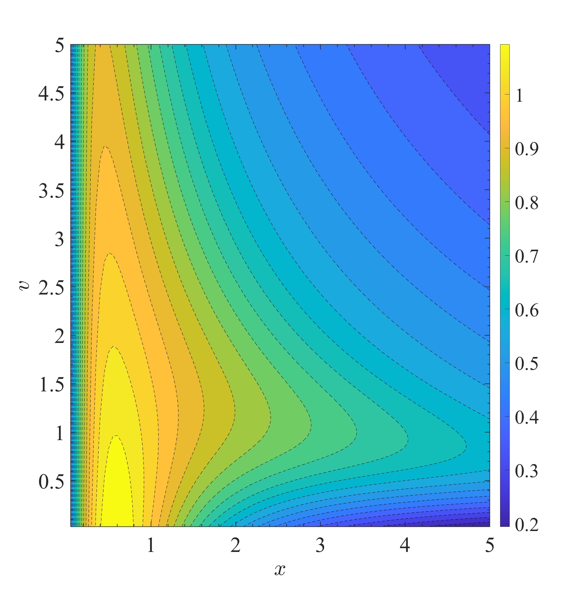
Figure 14: Contour plot of $F_{\text{DTL-A}}(x,v)$ given by Eq. (213).

Then the angular chirp strength introduced by a DTL compared to the energy chirp strength introduced by a single TEM00 laser modulator, i.e., that given in Eq. (167), with the same laser parameters and undulator length can be expressed as

$$\frac{t}{h}=\frac{F_{\text{DTL-A}}\left(\frac{L_{u}}{2Z_{R}},\frac{k_{L}Z_{R}\theta^{2}}{2}\right)}{\frac{\tan^{-1}\left(\frac{L_{u}}{2Z_{R}}\right)}{\sqrt{\frac{L_{u}}{2Z_{R}}}}}\frac{K[JJ]}{K[JJ]|_{\theta=0}}\theta.$$ (214)

Note that $K[JJ]$ in the numerator is a function of $\theta$. Since $\frac{F_{\text{DTL-A}}\left(\frac{L_{u}}{2Z_{R}},\frac{k_{L}Z_{R}\theta^{2}}{2}\right)}{\frac{\tan^{-1}\left(\frac{L_{u}}{2Z_{R}}\right)}{\sqrt{\frac{L_{u}}{2Z_{R}}}}}\frac{K[JJ]}{K[JJ]|_{\theta=0}}\sim 1$, and $\theta$ is usually in mrad level, given the same laser power, the DTL-induced angular chirp strength will be much smaller than the energy modulation strength induced by a TEM00 mode laser. This observation has been supported by more quantitative calculation of the angular chirp strength induced by DTL as shown in Fig. 15. As before, we have considered the case of keeping $\lambda_{u}$ or $B_{0}$ unchanged when we change the crossing angle $\theta$. In both cases, the maximal angular chirp strength induced with $P_{L}=1$ MW is about $t\approx 1.7$ $\text{m}^{-1}$. While from the evaluation below Fig. 8, at the same power level, a TEM00 mode laser modulation can induce an energy chirp strength of $h\sim 955\ \text{m}^{-1}$. This as explained is because $\theta$ is only $1\sim 2$ mrad. So we can see that the DTL-induced angular chirp strength, although a factor of three larger than that induced by a single normally incident TEM01 mode laser with the same laser power, is still generally quite small. There are two reasons why DTL is not very effective in imprinting angular modulation:

• The crossing angle between the laser and the electron propagating directions lead to the fact that they have a rather limited effective interaction region. For example, if the crossing angle is $\theta=5$ mrad, and the undulator length is $L_{u}=0.8$ m. Then the center of electron beam and center of laser beam at the undulator entrance and exit depart from each other with a distance of $\frac{L_{u}}{2}\theta=2$ mm, which is a large value compared to the laser beam waist $w_{0}=\sqrt{\frac{Z_{R}\lambda_{L}}{\pi}}\approx\sqrt{\frac{L_{u}\lambda_{L}}{2\pi}}=368\ \mu$m and results in a very weak laser electric field felt by the electron there.

• The decrease of undulator parameter $K$ with the increase of $\theta$ to meet the off-axis resonance condition, as can be seen in Figs. 10 and 12.

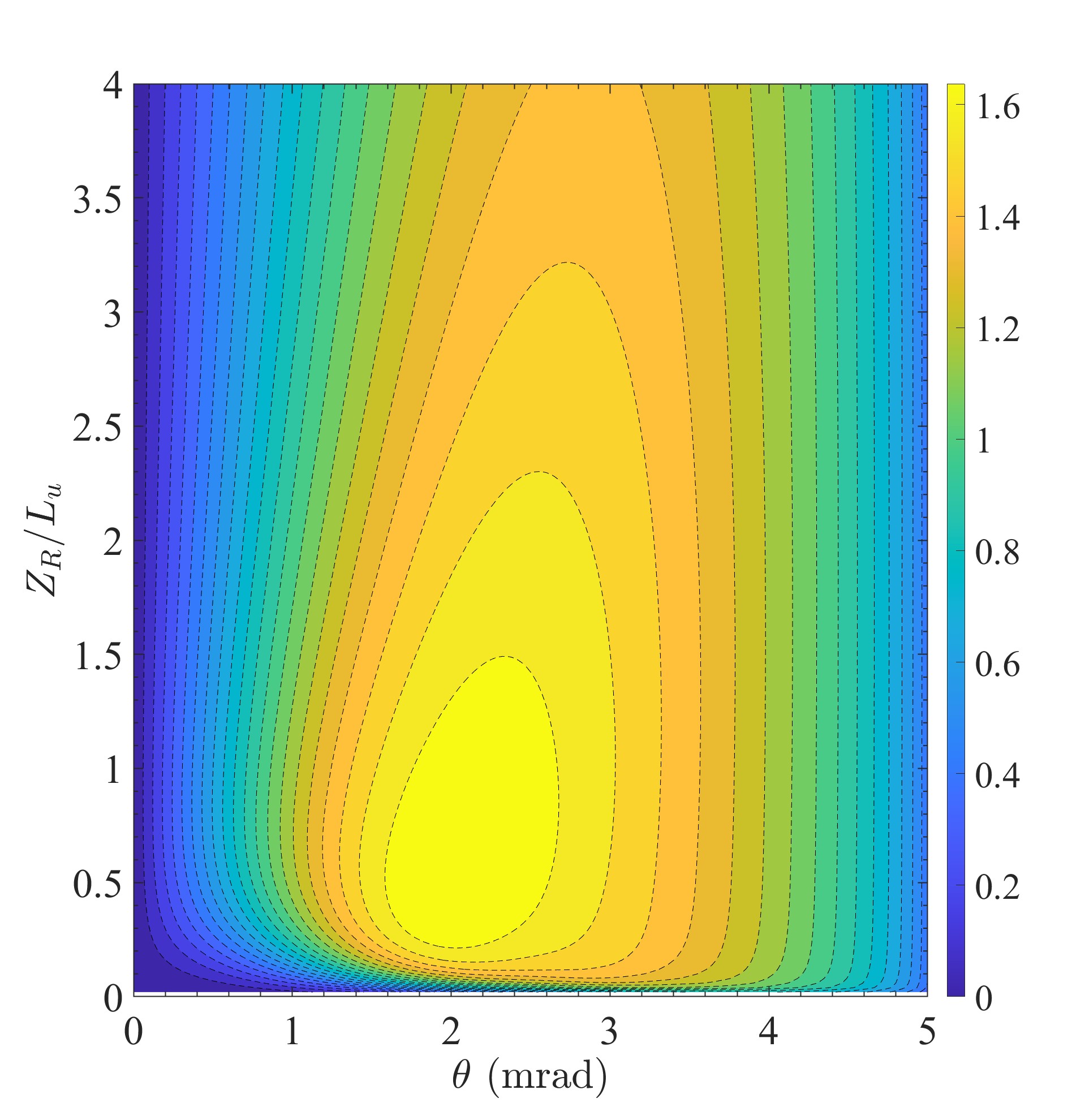
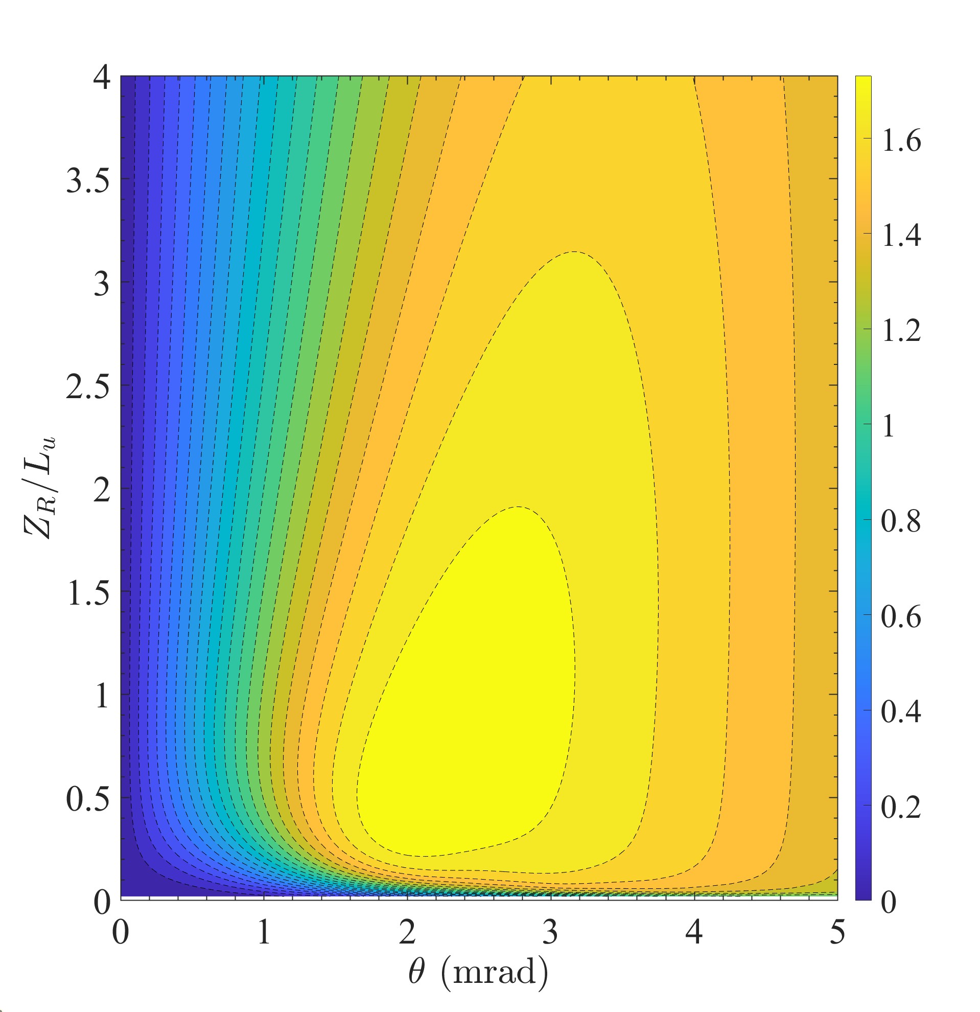
Figure 15: Left: Angular chirp strength $t$ v.s. $\theta$ and $Z_{R}/L_{u}$, keep $\lambda_{u}$ fixed when changing $\theta$. Parameters used: $E_{0}=600$ MeV, $\lambda_{L}=1064$ nm, $P_{L}=1$ MW, $\lambda_{u}=0.08$ m, $N_{u}=10$, $L_{u}=0.8$ m. Right: Angular chirp strength $t$ v.s. $\theta$ and $Z_{R}/L_{u}$, keep $B_{0}$ fixed when changing $\theta$. Parameters used: $E_{0}=600$ MeV, $\lambda_{L}=1064$ nm, $P_{L}=1$ MW, $B_{0}=1.2$ T, $L_{u}=0.8$ m.

Since the angular chirp strength is small, then according to Theorem Two, the required vertical beta function at the modulator $\beta_{y\text{M}}$ will be large. For example, if $\epsilon_{y}=4$ pm, $\sigma_{z\text{R}}=\sqrt{\epsilon_{y}\mathcal{H}_{y\text{R}}}=2$ nm, and $t=2\ \text{m}^{-1}$, then we need $\beta_{y\text{M}}=2.5\times 10^{5}$ m, which is too large to be used in practice. If we want to lower $\beta_{y\text{M}}$, it then means a higher modulation laser power is needed. This is the reason why we tend to use energy modulation-based coupling scheme for bunch compression or microbunching generation in GLSF SSMB.

Generally, when we compare the energy modulation-based and DTL-induced angular modulation-based bunch compression schemes, from the Theorem One and Two, i.e., Eqs. (93) and (95), for the same modulation laser wavelength $\lambda_{L}$ and power $P_{L}$, vertical emittance $\epsilon_{y}$ and target linear bunch length at the radiator $\sigma_{z\text{R}}=\sqrt{\epsilon_{y}\mathcal{H}_{y\text{R}}}$, we have

$$\beta_{y\text{M}}({\text{Angular modulation}})\sim\frac{\mathcal{H}_{y\text{M}}({\text{Energy modulation}})}{\theta^{2}}.$$ (215)

7 Applications in SSMB

Our goal in this paper is to find a solution for 1 kW EUV source based on SSMB, using parameters within the reach of present technology. According to our analysis, generalized longitudinal strong focusing (GLSF) turns out to be the most promising scenario, compared to longitudinal weak focusing and longitudinal strong focusing, in accomplishing this goal. The key of a GLSF SSMB ring is the precision transverse-longitudinal coupling dynamics to utilize the ultrasmall natural vertical emittance in a planar electron storage ring for efficient microbunching formation. For our purpose we find energy modulation-based coupling schemes are preferred than angular modulation-based coupling ones, in lowering the required modulation laser power. So the conclusion is that we will use energy modulation-based coupling scheme in a GLSF SSMB storage ring. In this section, we first present other various important physical considerations for a GLSF SSMB storage ring. Along with the previous analysis, an example parameters set of a 1 kW-average-power EUV source is then presented, as a summary of our investigation in this paper. As mentioned before, we will use a beam energy of $E_{0}=600$ MeV and laser wavelength of $\lambda_{L}=1064$ nm.

7.1 Various Physical Considerations

In GLSF scheme, a small vertical emittance is crucial. We assume that the vertical emittance used to accomplish our goal stated above is $\epsilon_{y}=40$ pm. One may notice that the vertical emittance we use is actually not extremely small. This conservative choice actually is a refection of consideration for intra-beam scattering (IBS) to be introduced soon. To realize significant coherent EUV generation, we may need to compress the linear bunch length $\sigma_{z\text{R}}=\sqrt{\epsilon_{y}\mathcal{H}_{y\text{R}}}$ to be as short as 2 nm, considering that we may generate microbunching based on a coasting beam or RF bunched beam in the ring. Then according to Eq. (146), the bunching factor at 13.5 nm is 0.0675. With $\epsilon_{y}=40$ pm, to get the desired linear bunch length at the radiator, we need $\mathcal{H}_{y\text{R}}=0.1\ \mu\text{m}.$ Such a precise control of $\mathcal{H}_{y\text{R}}$ is challenging but realizable using present technology.

7.1.1 Quantum Excitation Contribution to Vertical Emittance

Now we consider the quantum excitation contribution of GLSF sections to vertical emittance. According to our Theorem One, i.e., Eq. (93), the modulator should be placed at a dispersive location if we use energy modulation-based coupling for bunch compression or harmonic generation. Therefore, the quantum excitation of all bend-like elements, like dipoles, modulators and radiator in the GLSF section, will contribute to the vertical emittance.

The contribution of a radiator to $\epsilon_{y}$ is

$$\Delta\epsilon_{y\text{R}} =\frac{55}{96\sqrt{3}}\frac{\alpha_{F}{\lambdabar}_{e}^{2}\gamma^{5}}{\alpha_{V}}\int_{0}^{L_{u}}\frac{\mathcal{H}_{y\text{R}}}{|\rho(s)|^{3}}ds$$ (216)

$$=\frac{55}{96\sqrt{3}}\frac{\alpha_{F}{\lambdabar}_{e}^{2}\gamma^{5}}{\alpha_{V}}\frac{\mathcal{H}_{y\text{R}}}{\rho_{0\text{R}}^{3}}\int_{0}^{L_{u\text{R}}}|\sin(k_{u}s)|^{3}ds$$

$$=\frac{55}{96\sqrt{3}}\frac{\alpha_{F}{\lambdabar}_{e}^{2}\gamma^{5}}{\alpha_{V}}\frac{\mathcal{H}_{y\text{R}}}{\rho_{0\text{R}}^{3}}\frac{4}{3\pi}L_{u\text{R}},$$

with

$$\alpha_{V}\approx\frac{U_{0}}{2E_{0}}=\frac{1}{2}C_{\gamma}\frac{E_{0}^{3}}{\rho_{\text{ring}}}=\frac{1}{2}C_{\gamma}\times 0.2998B_{\text{ring}}[\text{T}]E_{0}^{2}[\text{GeV}]$$ (217)

with $C_{\gamma}=8.85\times 10^{-5}\frac{\text{m}}{\text{GeV}^{3}}$. Note that here we have assumed that the radiation energy loss in the GLSF section is much less than that induced by the bending magnets in the ring, thus that the damping rate is determined by the ring dipoles. In a more easy to use form we have

$$\Delta\epsilon_{y\text{R}}[\text{nm}] =8.9B_{\text{ring}}^{-1}[\text{T}]B_{0\text{R}}^{3}[\text{T}]\mathcal{H}_{y\text{R}}[\text{m}]L_{u\text{R}}[\text{m}],$$ (218)

where $B_{0\text{R}}$ and $L_{u\text{R}}$ are the peak magnetic field and length of the radiator undulator. For example, if $B_{\text{ring}}=1.33$ T, $\lambda_{u\text{R}}=1.8$ cm ($B_{0\text{R}}=0.867$ T), $\mathcal{H}_{y\text{R}}=0.1\ \mu$m, $L_{u\text{R}}=5.69$ m ($N_{u}=4\times 79$) , then $\Delta\epsilon_{y\text{R}}=2.5$ fm, which is much less than $\epsilon_{y}$. Generally, since $\mathcal{H}_{y}$ at the radiator is quite small, the contribution of radiator to vertical emittance is not the dominant one, compared to that from modulators and dipoles to be introduced.

Similar to the analysis for radiator, the contribution of two GLSF modulators to $\epsilon_{y}$ is:

$$\Delta\epsilon_{y\text{M}}[\text{nm}] =17.8B_{\text{ring}}^{-1}[\text{T}]B_{0\text{M}}^{3}[\text{T}]\mathcal{H}_{y\text{M}}[\text{m}]L_{u\text{M}}[\text{m}],$$ (219)

where $B_{0\text{R}}$ and $L_{u\text{R}}$ are the peak magnetic field and length of the modulator undulators. For example, if the parameters of the modulators are that given in Tab. 2, where $B_{\text{ring}}=1.33$ T, $B_{0\text{M}}=0.806$ T, $\mathcal{H}_{y\text{M}}=0.056$ m, $L_{u\text{M}}=1.6$ m, then $\Delta\epsilon_{y\text{M}}=631$ pm, which is a quite large value compared to that contributed from radiator. This is mainly due to the fact that $\mathcal{H}_{y\text{M}}\gg\mathcal{H}_{y\text{R}}$. As we will introduce soon, we can apply the damping wiggler to control this contribution by increasing the radiation damping rate.

There are also vertical dipoles in the GLSF section for optics manipulation to fulfill the bunch compression or harmonic generation condition. But in principle we can use weak dipole field to minimize their contribution to vertical emittance, and satisfy the symplectic optics requirement at the same time. Of course, the total length of these dipoles should not be too long.

In our present evaluation, we will assume that the contribution from modulators are the dominant one if we consider single-particle dynamics alone. We need $\Delta\epsilon_{y\text{M}}<\epsilon_{y}$. It would be better if $\Delta\epsilon_{y\text{M}}$ is only a small portion of $\epsilon_{y}$, since then it leaves more room for other contribution of vertical emittance, like IBS and that from $x$-$y$ coupling. In principle, we can also use a weaker modulator field to weaken quantum excitation, but this also means the laser-electron interaction will be less efficient, and a larger laser power is needed if we want to imprint the same energy modulation strength.

7.1.2 Application of Damping Wiggler

To speed up damping, which is helpful in controling the vertical emittance growth from quantum excitation and IBS, we may invoke damping wiggler. We can put a horizontal damping wiggler or several wigglers at dispersion-free locations. In such a way, the damping wiggler will contribute only damping and no excitation to the vertical emittance. Assuming that

$$\Delta U_{0\text{W}}=R_{\text{W}}U_{0\text{dipoles}},$$ (220)

with $U_{0\text{dipoles}}=C_{\gamma}\frac{E_{0}^{4}}{\rho_{\text{ring}}}$ the radiation energy loss per particle from the bending magnets in the ring, $\Delta U_{0\text{W}}$ radiation loss from the damping wiggler, and

$$R_{\text{W}}=\frac{\Delta U_{0\text{W}}}{U_{0\text{dipoles}}}=\frac{1}{2}\left(\frac{B_{0\text{W}}}{B_{\text{ring}}}\right)^{2}\frac{L_{u\text{W}}}{2\pi\rho_{\text{ring}}},$$ (221)

where $B_{0\text{W}}$ and $L_{u\text{W}}$ are the peak magnetic field and length of the damping wiggler, respectively. Since the damping rate is proportional to the radiation energy loss per turn, then the damping constant will be a factor of $R_{\text{W}}$ larger by applying the damping wiggler

$$\alpha_{V}=(1+R_{\text{W}})\alpha_{V0},$$ (222)

with $\alpha_{V0}$ the natural vertical damping rate without damping wiggler. Then the above evaluated emittance growth from radiaotr, modulators and dipoles will become $\frac{1}{1+R_{\text{W}}}$ of the original value. For example for the modulators, we have

$$\Delta\epsilon_{y\text{M}}[\text{nm}] =\frac{1}{1+R_{\text{W}}}17.8B_{\text{ring}}^{-1}[\text{T}]B_{0\text{M}}^{3}[\text{T}]\mathcal{H}_{y\text{M}}[\text{m}]L_{u\text{M}}[\text{m}].$$ (223)

Put the above relation in another way

$$L_{u\text{M}}[\text{m}]\approx 56.2\left(1+R_{\text{W}}\right)\frac{B_{\text{ring}}[\text{T}]\Delta\epsilon_{y\text{M}}[\text{pm}]}{\mathcal{H}_{y\text{M}}[\mu\text{m}]B_{0\text{M}}^{3}[\text{T}]}.$$ (224)

We will use a rather strong and rather long superconducting damping wiggler to speed up damping to fight against the IBS diffusion and quantum excitation to maintain a small vertical emittance. For example, if $B_{0\text{W}}=6$ T and $L_{u\text{W}}=60$ m, then $U_{0\text{W}}=492$ keV and $R_{\text{W}}=64.4$. By applying such a strong damping wiggler, we now have $\Delta\epsilon_{y\text{M}}=9.65$ pm, which is a factor of four smaller than the desired 40 pm vertical emittance and should be acceptable. Assuming the circumference of the ring is 200 m, he longitudinal and vertical radiation damping time are correspondingly

$$\tau_{\delta\text{RD}}=0.81\ \text{ms},\ \tau_{y\text{RD}}=1.63\ \text{ms}.$$ (225)

We will compare this radiation damping speed with the IBS diffusion later.

For completeness of discussion, we remind the readers that the damping wiggler also has quantum excitation, in particular to energy spread. Considering both the ring dipoles and damping wiggler, the new equilibrium energy spread is

$$\sigma_{\delta,\text{new}}=\sigma_{\delta 0}\sqrt{\frac{1+\frac{4}{3\pi}\left(\frac{B_{0\text{W}}}{B_{\text{ring}}}\right)^{3}\frac{L_{u}}{2\pi\rho_{\text{ring}}}}{1+\frac{1}{2}\left(\frac{B_{0\text{W}}}{B_{\text{ring}}}\right)^{2}\frac{L_{u}}{2\pi\rho_{\text{ring}}}}},$$ (226)

where

$$\sigma_{\delta 0}=\sqrt{\frac{C_{q}}{J_{s}}\frac{\gamma^{2}}{\rho_{\text{ring}}}}$$ (227)

is the natural energy spread if there is no damping wiggler, with $C_{q}=\frac{55\lambdabar_{e}}{32\sqrt{3}}=3.8319\times 10^{-13}$ m, ${\lambdabar}_{e}=\frac{\lambda_{e}}{2\pi}=386$ fm is the reduced Compton wavelength of electron, $J_{s}=2+\mathcal{D}$ is the longitudinal damping partition number, $\gamma$ is the Lorentz factor. Nominally, we have $J_{s}\approx 2$. So

$$\sigma_{\delta 0}\approx 4.69\times 10^{-4}B^{\frac{1}{2}}_{\text{ring}}[\text{T}]E_{0}^{\frac{1}{2}}[\text{GeV}].$$ (228)

For example, if $B_{0\text{W}}=1.33$ T, and $E_{0}=600$ MeV, then $\sigma_{\delta 0}=4.2\times 10^{-4}$. When $\frac{1}{2}\left(\frac{B_{0\text{W}}}{B_{\text{ring}}}\right)^{2}\frac{L_{u}}{2\pi\rho_{\text{ring}}}\gg 1$ and $\frac{4}{3\pi}\left(\frac{B_{0\text{W}}}{B_{\text{ring}}}\right)^{3}\frac{L_{u}}{2\pi\rho_{\text{ring}}}\gg 1$, which means the energy spread is dominant by the damping wiggler, we have

$$\sigma_{\delta,\text{new}}\approx\sigma_{\delta 0}\sqrt{\frac{8}{3\pi}\frac{B_{0\text{W}}}{B_{\text{ring}}}}=\sqrt{\frac{8}{3\pi}\frac{C_{q}}{J_{s}}\frac{\gamma^{2}}{\rho_{0\text{W}}}}\approx 4.32\times 10^{-4}B^{\frac{1}{2}}_{0\text{W}}[\text{T}]E_{0}^{\frac{1}{2}}[\text{GeV}].$$ (229)

So given the beam energy, the new equilibrium energy spread will depends solely on the peak magnetic field of the damping wiggler $B_{0\text{W}}$. For example, if $E_{0}=600$ MeV and $B_{0\text{W}}=6$ T, then the asymptotic energy spread is $\sigma_{\delta,\text{new}}=8.2\times 10^{-4}$.

7.1.3 Intra-beam Scattering

We mentioned that our conservative choice of $\epsilon_{y}=40$ pm is mainly from the consideration of intra-beam scattering (IBS). Now this can be understood with more quantitative calculations. We will see that IBS turns out to the most fundamental obstacle in obtaining the ultrasmall vertical emittance in GLSF SSMB. This is partially because our choice of beam energy is not too high. In addition, to realize high EUV power, we need a high peak current which means a high charge density in phase space.

We use Bane’s high energy approximation [33] to calculate the IBS diffusion rate

$$\frac{1}{T_{\delta}} \approx\frac{r_{e}^{2}cNL_{c}}{16\gamma^{3}\epsilon_{x}^{\frac{3}{4}}\epsilon_{y}^{\frac{3}{4}}\sigma_{z}\sigma_{\delta}^{3}}\left\langle\sigma_{H}g_{\text{Bane}}\left(\frac{a}{b}\right)\left(\beta_{x}\beta_{y}\right)^{-\frac{1}{4}}\right\rangle,$$ (230)

$$\frac{1}{T_{x,y}} =\frac{\sigma_{\delta}^{2}\langle\mathcal{H}_{x,y}\rangle}{\epsilon_{x,y}}\frac{1}{T_{\delta}},$$

$$\frac{1}{\sigma_{H}^{2}} =\frac{1}{\sigma_{\delta}^{2}}+\frac{\mathcal{H}_{x}}{\epsilon_{x}}+\frac{\mathcal{H}_{y}}{\epsilon_{y}},$$

$$g_{\text{Bane}}(\alpha) =\frac{2\sqrt{\alpha}}{\pi}\int_{0}^{\infty}\frac{du}{\sqrt{1+u^{2}}\sqrt{\alpha^{2}+u^{2}}},$$

$$a =\frac{\sigma_{H}}{\gamma}\sqrt{\frac{\beta_{x}}{\epsilon_{x}}},\ b=\frac{\sigma_{H}}{\gamma}\sqrt{\frac{\beta_{y}}{\epsilon_{y}}}.$$

where $r_{e}=2.818\times 10^{-15}$ m is the classical electron radius and $L_{c}$ is the Coulomb Log. $N$ is the number of electrons in the bunch. For a coasting beam, we need to replace $\sigma_{z}\rightarrow L/(2\sqrt{\pi})$ where $L$ is the bunch length. Note that $\frac{eN}{L/c}=I_{P}$ according to our definition, where $I_{P}$ is the peak current.

Now we put in some example numbers to do an estimation for the IBS diffusition rate in a GLSF EUV SSMB ring:

$$E_{0} =600\ \text{MeV},\ I_{P}=40\ \text{A},\ \sigma_{\delta}=8.5\times 10^{-4},\ \epsilon_{x}=2\ \text{nm},\ \epsilon_{y}=40\ \text{pm},$$ (231)

$$\langle\sigma_{H}\rangle =4\times 10^{-5},\ \frac{a}{b}=\frac{1}{10},\ g_{\text{Bane}}\left(\frac{1}{10}\right)=0.744,\ \langle\left(\beta_{x}\beta_{y}\right)^{-\frac{1}{4}}\rangle=0.32,$$

$$\langle\mathcal{H}_{y}\rangle =\frac{2\times 1.6\times 0.056\ \text{m}}{200}=0.9\ \text{mm},\ L_{c}=10.$$

Note that $\mathcal{H}_{y}=0.056$ m at the two modulators, whose length are both 1.6 m. In evaluating $\langle\mathcal{H}_{y}\rangle$ we have only considered the contribution from modulators. This is a simplification, but should give a correct order of magnitude estimation. Putting in the example numbers, we then have

$$\tau_{\delta\text{IBS}} =113\ \text{ms},\ \tau_{y\text{IBS}}=7\ \text{ms}.$$ (232)

Compared with the radiation damping times given in Eq. (225), we can see that even for the vertical dimension, the IBS diffusion is more than four times slower than radiation damping. Therefore, the IBS diffusion can now be controlled by the strong damping induced by the damping wiggler. This calculation also justifies the necessity or gain of applying damping wiggler.

7.1.4 Microwave Instability

Now we want to evaluate if the peak current of 40 A we apply in the above example is doable. One of the main limitation of peak current is the microwave instability induced by coherent synchrotron radiation (CSR). According to Ref. [34], the CSR-induced microwave instability threshold is

$$(S_{\text{CSR}})_{\text{th}}=0.5+0.12\Pi,$$ (233)

with

$$S_{\text{CSR}}=\frac{I\rho^{1/3}}{\sigma_{z0}^{4/3}},\ I=\frac{r_{e}N_{b}}{2\pi\nu_{s0}\gamma\sigma_{\delta 0}},\ \Pi=\frac{\sigma_{z0}\rho^{1/2}}{g^{3/2}},$$ (234)

and $2g$ is the separation between the two plates. So the threshold peak current is

$$I_{\text{th,peak}} =\frac{eN_{b}}{\sqrt{2\pi}\sigma_{z0}/c}$$ (235)

$$=\frac{\sqrt{2\pi}ec\nu_{s0}\gamma\sigma_{\delta 0}\sigma_{z0}^{1/3}}{r_{e}\rho^{1/3}}\left(0.5+0.12\frac{\sigma_{z0}\rho^{1/2}}{g^{3/2}}\right)$$

$$=\frac{1}{2\sqrt{2\pi}}I_{Alf}\gamma\left(1+0.24\frac{\sigma_{z0}\rho^{1/2}}{g^{3/2}}\right)\frac{\sigma_{\delta 0}^{2}|R_{56}|}{(\rho\sigma_{z0}^{2})^{1/3}}$$

$$=\frac{1}{2\sqrt{2\pi}}I_{Alf}\gamma\left(1+0.24\frac{\sigma_{\delta 0}|R_{56}|^{1/2}\rho^{1/2}}{|h|^{1/2}g^{3/2}}\right)\frac{\sigma_{\delta 0}^{\frac{4}{3}}|R_{56}|^{\frac{2}{3}}|h|^{\frac{1}{3}}}{\rho^{1/3}},$$

with $I_{Alf}=\frac{ec}{r_{e}}=17$ kA being the Alfven current. The $R_{56}=-\eta C_{0}$ is that of the whole ring. $h=\frac{eV_{RF}\cos\phi_{s}}{E_{0}}k_{L}$ is the linear energy chirp strength around the synchronous RF phase. Putting in some typical parameters for the EUV SSMB: $E_{0}=600$ MeV, $B_{0}=1.33$ T, $\rho=1.5$ m, $R_{56}=1$ m, $\sigma_{\delta 0}=8.5\times 10^{-4}$, $g=4$ cm, $h=0.01\ \text{m}^{-1}$ (about 600 kV voltage for a 500 MHz RF) then

$$I_{\text{th,peak}}=60.3\times\left(1+0.31\right)\ \text{A}=79\ \text{A}.$$ (236)

So our application of a peak current of 40 A should be safe from microwave instability.

We remind the readers that in this evaluation, we actually assumed that the beam is RF bunched. While in our evaluation of IBS, we have assumed that the beam is a coasting beam. These evaluations here mainly serve as an order of magnitude estimation that support the general feasibility of our parameter choice. A more detailed analysis of collective effects will be necessary in the future development of such a GLSF SSMB light source.

7.1.5 Modulation Laser Power

Now we evaluate the modulation laser power required. Given the laser wavelength, modulator undulator parameters and the required energy chirp strength, we can use Eq. (167) to calculate the required laser power

$$P_{L}=\frac{\lambda_{L}}{4Z_{0}Z_{R}}\left(h\frac{1}{\frac{eK[JJ]}{\gamma^{2}m_{e}c^{2}}\tan^{-1}\left(\frac{L_{u}}{2Z_{R}}\right)k_{L}}\right)^{2}.$$ (237)

Using Theorem one, i.e., Eq. (93), and let the equality in the relation holds, we have

$$P_{L} =\frac{\lambda_{L}}{4Z_{0}Z_{R}}\left(\frac{1}{\sqrt{\mathcal{H}_{y\text{M}}\mathcal{H}_{y\text{R}}}}\frac{1}{\frac{eK[JJ]}{\gamma^{2}m_{e}c^{2}}\tan^{-1}\left(\frac{L_{u}}{2Z_{R}}\right)k_{L}}\right)^{2}$$ (238)

$$=\frac{\lambda_{L}}{4Z_{0}Z_{R}}\frac{\epsilon_{y}}{\mathcal{H}_{y\text{M}}}\left(\frac{1}{\sigma_{z\text{R}}}\frac{1}{\frac{eK[JJ]}{\gamma^{2}mc^{2}}\tan^{-1}\left(\frac{L_{u}}{2Z_{R}}\right)k_{L}}\right)^{2}$$

$$=\frac{\lambda_{L}^{3}}{4\pi^{2}4Z_{0}Z_{R}}\frac{\epsilon_{y}}{\frac{\Delta\epsilon_{y\text{M}}}{2\times\frac{55}{96\sqrt{3}}\frac{\alpha_{F}{\lambdabar}_{e}^{2}\gamma^{5}}{\alpha_{V}}\frac{1}{\rho_{0\text{M}}^{3}}\frac{4}{3\pi}L_{u}}}\left(\frac{1}{\sigma_{z\text{R}}}\frac{1}{\frac{eK[JJ]}{\gamma^{2}mc^{2}}\tan^{-1}\left(\frac{L_{u}}{2Z_{R}}\right)}\right)^{2}$$

$$=\frac{\epsilon_{y}}{\Delta\epsilon_{y\text{M}}}\frac{\lambda_{L}^{3}}{3\pi^{3}Z_{0}}\frac{55}{96\sqrt{3}}\frac{\alpha_{F}{\lambdabar}_{e}^{2}\gamma^{5}}{\alpha_{V}}\frac{1}{\rho_{0\text{M}}^{3}}\frac{L_{u}}{2Z_{R}}\left(\frac{1}{\sigma_{z\text{R}}}\frac{1}{\frac{eK[JJ]}{\gamma^{2}mc^{2}}\tan^{-1}\left(\frac{L_{u}}{2Z_{R}}\right)}\right)^{2}$$

$$=\frac{1}{1+R_{\text{W}}}\frac{\epsilon_{y}}{\Delta\epsilon_{y\text{M}}}\frac{\lambda_{L}^{3}}{3\pi^{3}Z_{0}}\frac{55}{48\sqrt{3}}\frac{\alpha_{F}{\lambdabar}_{e}^{2}\gamma^{7}B^{3}_{0\text{M}}}{C_{\gamma}E_{0}P^{2}_{0}B_{\text{ring}}}\frac{1}{\sigma_{z\text{R}}^{2}}\frac{\frac{L_{u}}{2Z_{R}}}{\left[K[JJ]\tan^{-1}\left(\frac{L_{u}}{2Z_{R}}\right)\right]^{2}}$$

$$\approx\frac{1}{1+R_{\text{W}}}\frac{\epsilon_{y}}{\Delta\epsilon_{y\text{M}}}\frac{\lambda_{L}^{3}}{3\pi^{3}Z_{0}}\frac{55}{48\sqrt{3}}\frac{c^{2}\alpha_{F}{\lambdabar}_{e}^{2}\gamma^{7}B^{3}_{0\text{M}}}{C_{\gamma}E^{3}_{0}B_{\text{ring}}}\frac{1}{\sigma_{z\text{R}}^{2}}\frac{\frac{L_{u}}{2Z_{R}}}{\left[K[JJ]\tan^{-1}\left(\frac{L_{u}}{2Z_{R}}\right)\right]^{2}}$$

$$=\frac{1}{1+R_{\text{W}}}\frac{\epsilon_{y}}{\Delta\epsilon_{y\text{M}}}\frac{1}{\left(K[JJ]\right)^{2}}\frac{\lambda_{L}^{3}}{3\pi^{3}Z_{0}}\frac{55}{48\sqrt{3}}\frac{\alpha_{F}c^{2}{\lambdabar}_{e}^{2}\gamma^{7}B^{3}_{0\text{M}}}{C_{\gamma}E^{3}_{0}B_{\text{ring}}}\frac{1}{\sigma_{z\text{R}}^{2}}\frac{\frac{L_{u}}{2Z_{R}}}{\left[\tan^{-1}\left(\frac{L_{u}}{2Z_{R}}\right)\right]^{2}},$$

where $R_{\text{W}}$ is given by Eq. (221). In the above derivation we have used the electron momentum $P_{0}=\gamma m_{e}c$ and approximation $E_{0}\approx P_{0}c$. Now we try to derive more useful scaling laws to offer guidance in our parameters choice for a GLSF SSMB storage ring. To maximize the energy modulation, we need $\frac{Z_{R}}{L_{u}}=0.359\approx\frac{1}{3}$. When $K>\sqrt{2}$, we approximate the resonance condition as $\lambda_{L}=\frac{1+\frac{K^{2}}{2}}{2\gamma^{2}}\lambda_{u}\approx\frac{K^{2}}{4\gamma^{2}}\lambda_{u},$ and $[JJ]\approx 0.7$. Then we have

$$P_{L} \propto\frac{1}{1+R_{\text{W}}}\frac{\epsilon_{y}}{\Delta\epsilon_{y\text{M}}}\frac{\lambda_{L}^{3}}{K^{2}}\frac{\gamma^{4}B^{3}_{0\text{M}}}{B_{\text{ring}}}\frac{1}{\sigma_{z\text{R}}^{2}}\propto\frac{1}{1+R_{\text{W}}}\frac{\epsilon_{y}}{\Delta\epsilon_{y\text{M}}}\frac{\lambda_{L}^{\frac{7}{3}}\gamma^{\frac{8}{3}}B^{\frac{7}{3}}_{0\text{M}}}{B_{\text{ring}}}\frac{1}{\sigma_{z\text{R}}^{2}}.$$ (239)

Putting in the numbers for the constants, we obtain the quantitative expressions of the above scalings for practical use

$$P_{L}[\text{kW}] \approx 5.7\frac{1}{1+R_{\text{W}}}\frac{\epsilon_{y}}{\Delta\epsilon_{y\text{M}}}\frac{\lambda_{L}^{\frac{7}{3}}[\text{nm}]E_{0}^{\frac{8}{3}}[\text{GeV}]B_{0\text{M}}^{\frac{7}{3}}[\text{T}]}{\sigma_{z\text{R}}^{2}[\text{nm}]B_{\text{ring}}[\text{T}]}.$$ (240)

The above scaling laws are accurate when $K>\sqrt{2}$. Note that the calculated power are the peak power of the laser. For completeness, here we give again the modulator length scaling

$$L_{u\text{M}}[\text{m}]\approx 56.2\left(1+R_{\text{W}}\right)\frac{B_{\text{ring}}[\text{T}]\Delta\epsilon_{y\text{M}}[\text{pm}]}{\mathcal{H}_{y\text{M}}[\mu\text{m}]B_{0\text{M}}^{3}[\text{T}]}.$$ (241)

Therefore, to lower the required modulation laser power, we can apply a large $R_{\text{W}}$, which means a strong damping wiggler. A short laser wavelength and low beam energy are also preferred. But their choices should take more factors into account, for example IBS and engineering experience of optical enhancement cavity. A strong bending magnet field in the ring is also desired. Concerning the modulator field strength, a weaker one is favored to lower the required laser power. But note that the required modulator length may be longer, if we keep $\Delta\epsilon_{y\text{M}}$ unchanged in this process.

7.1.6 Radiation Power

Having formed the microbunching, now comes the radiation generation. We will use a planar undulator as the radiator. Coherent undulator radiation power at the odd-$H$-th harmonic from a transversely-round electron beam is [8]

$$P_{H,\text{peak}}[\text{kW}]=1.183N_{u}H\chi[JJ]_{H}^{2}FF_{\bot}(S)|b_{z,H}|^{2}I_{P}^{2}[\text{A}],$$ (242)

where $N_{u}$ is the number of undulator periods, $[JJ]_{H}^{2}=\left[J_{\frac{H-1}{2}}\left(H\chi\right)-J_{\frac{H+1}{2}}\left(H\chi\right)\right]^{2}$, with $\chi=\frac{K^{2}}{4+2K^{2}}$, and the transverse form factor is

$$FF_{\bot}(S)=\frac{2}{\pi}\left[\tan^{-1}\left(\frac{1}{2S}\right)+S\ln\left(\frac{(2S)^{2}}{(2S)^{2}+1}\right)\right],$$ (243)

with $S=\frac{\sigma^{2}_{\bot}\frac{\omega}{c}}{L_{u}}$ and $\sigma_{\bot}$ the RMS transverse electron beam size, $b_{z,H}$ is the bunching factor at the $H$-th harmonic decided by the longitudinal current distribution, and $I_{P}$ is the peak current.

The above formula is derived by assuming that the longitdudinal and transverse distribution of the electron beam do not change much in the radiator. Actually the energy spread of electron beam can lead to current distribution change inside the undulator, considering that the undulator has an $R_{56}=2N_{u}\lambda_{0}$, where $\lambda_{0}$ is the fundamental on-axis resonant wavelength of the undulator. If we consider the impact of energy spread on coherent radiation, and assuming that the microbunching length reach its minimum at the radiator center, there will be a correction or reduction factor to the radiation power given by Eq. (242)

$$\mathcal{R}=\frac{\sqrt{\pi}}{2}\frac{\text{erf}\left(\frac{\omega}{c}\sigma_{\delta}N_{u}\lambda_{0}\right)}{\frac{\omega}{c}\sigma_{\delta}N_{u}\lambda_{0}}.$$ (244)

Here we remind the readers that in our case of GLSF SSMB, the beam is actually not transversely round in the radiator. Therefore, we have used an effective round beam size in evaluating the radiation power using the above formula. This effective transverse beam size $\sigma_{\bot}$ is in between $\sigma_{x}$ and $\sigma_{y}$.

7.1.7 Wiggling of $\mathcal{H}_{y}$ Inside an Undulator

In the previous sections, we have evaluated the quantum excitation contribution of GLSF modulators and radiator. However, we have assumed $\mathcal{H}_{y}$ is a constant value all through the undulator. This is actually not true strictly speaking. In this section, we study the wiggling of $\mathcal{H}_{y}$ due to the intrinsic dispersion inside a planar vertical undulator. We set the undulator center to be $s=0$. The linear transfer matrix of a vertical planar undulator from $s=0$ to $s\in[-\frac{L_{u}}{2},\frac{L_{u}}{2}]$ is [35]

$${\bf U}(s,0)=\left(\begin{matrix}\cos(k_{y}s)&\frac{\sin(k_{y}s)}{k_{y}}&0&0&0&0\\ -k_{y}\sin(k_{y}s)&\cos(k_{y}s)&0&0&0&0\\ 0&0&1&s&0&-\frac{K}{\gamma k_{u}}[1-\cos(k_{u}s)]\\ 0&0&0&1&0&-\frac{K}{\gamma}\sin(k_{u}s)\\ 0&0&U_{53}&U_{54}&1&U_{56}\\ 0&0&0&0&9&1\end{matrix}\right)$$ (245)

where $U_{53}=-U_{46}$, $U_{54}=-sU_{46}+U_{36}$ and $U_{56}=\frac{2\lambda_{0}}{\lambda_{u}}s+\frac{K^{2}}{\gamma^{2}}\left[\frac{\sin(2k_{u}s)-4\sin(k_{u}s)}{4k_{u}}\right],$ with $\lambda_{0}=\frac{1+K^{2}/2}{2\gamma^{2}}\lambda_{u}$ being the fundamental on-axis resonant wavelength. Eigenvector of one-turn map corresponding to the vertical mode at the undulator entrance is

$${\bf E}_{II}(0)=\frac{1}{\sqrt{2}}\left(\begin{matrix}0\\ 0\\ \sqrt{\beta_{y0}}\\ \frac{i-\alpha_{y0}}{\sqrt{\beta_{y0}}}\\ -\sqrt{\beta_{y0}}D_{y0}^{\prime}+\frac{i-\alpha_{y0}}{\sqrt{\beta_{y0}}}D_{y0}\\ 0\end{matrix}\right)e^{i\Phi_{II0}}.$$ (246)

For the GLSF modulator, $\mathcal{H}_{y0}$ at the undulator center is

$$\mathcal{H}_{y0}\equiv 2|E_{II5}(0)|^{2}=\frac{D_{y0}^{2}+\left(\alpha_{y0}D_{y0}+\beta_{y0}D_{y0}^{\prime}\right)^{2}}{\beta_{y0}}$$ (247)

The evolution of $\mathcal{H}_{y}$ from $s=0$ to $s$ is

$$\mathcal{H}_{y}(s) \equiv 2|E_{II5}(s)|^{2}=2|\left({\bf U}(s,0){\bf E}_{II}(0)\right)_{5}|^{2}$$ (248)

$$=\frac{(D_{y0}+U_{36}-U_{46}s)^{2}+\left[\alpha_{y0}(D_{y0}+U_{36}-U_{46}s)+\beta_{y0}(D_{y0}^{\prime}+U_{46})\right]^{2}}{\beta_{y0}}.$$

Since $|hR_{56}|\ll 1$ for the modulator, where $h$ and $R_{56}$ are the energy chirp strength induced by and $R_{56}$ of the modulator, we can approximately use the transfer matrix of the undulator alone to describe the evolution of $\mathcal{H}_{y}$ inside the GLSF modulator. The left part of Fig. 16 is an example plot of $\mathcal{H}_{y}$ inside the modulator, if vertical undulator is used. As can be seen, since $\mathcal{H}_{y}$ at the modulator is generally quite large, the relative wiggling of $\mathcal{H}_{y}$ in the modulator is small.

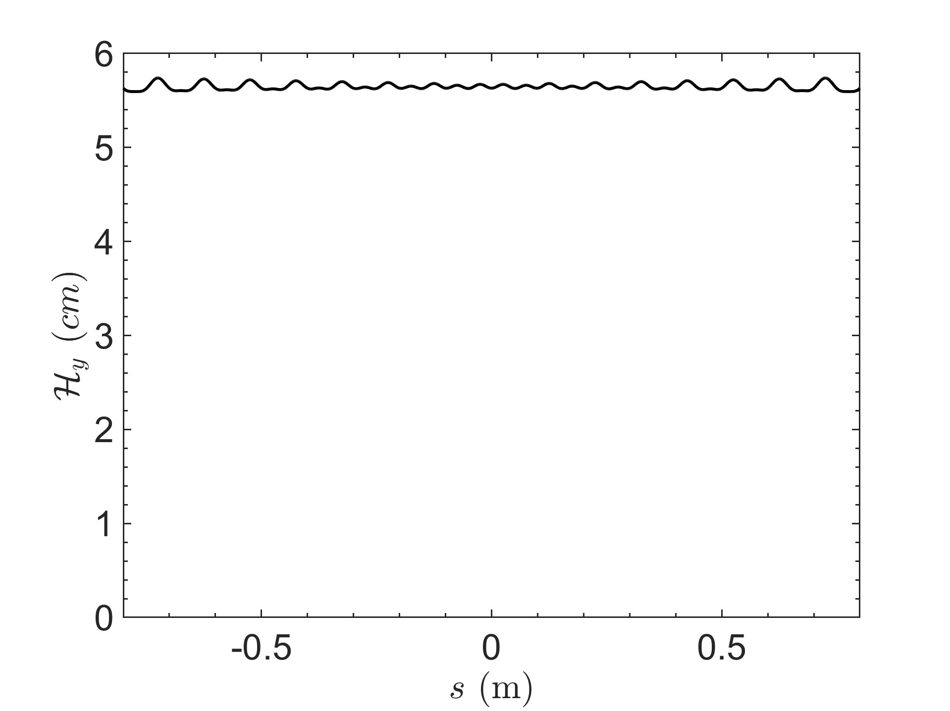
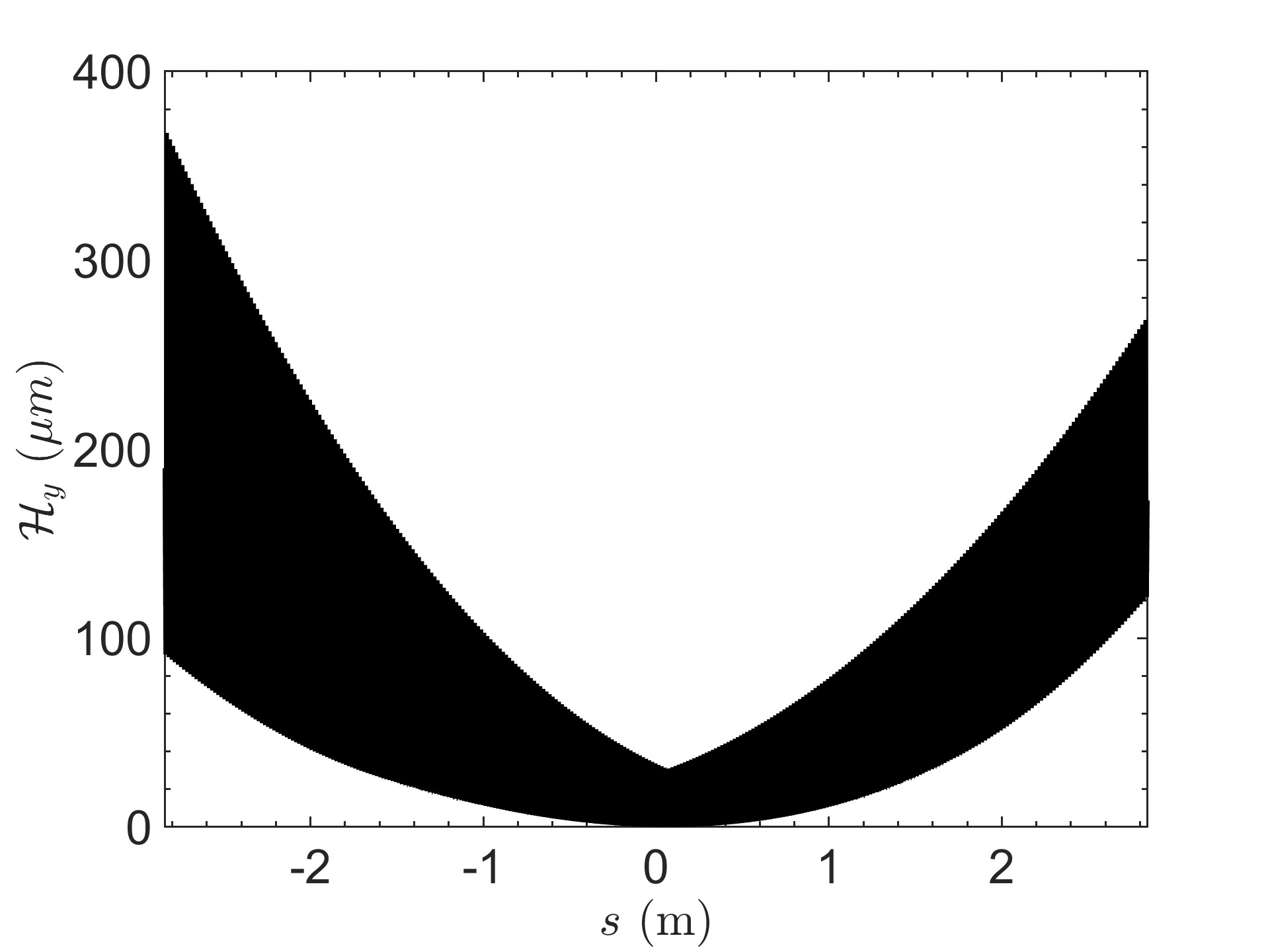
Figure 16: Left: an example evolution of $\mathcal{H}_{x}$ inside the GLSF modulator if vertical undulator is used. Right: an example evolution of $\mathcal{H}_{x}$ inside the GLSF radiator if vertical undulator is used. Undulator parameters as given in Tab. 2. Twiss parameters at the modulator center used for calculation: $D_{y0}=0.75$ m, $D_{y}^{\prime}=0$, $\alpha_{y0}=0$, $\beta_{y0}=10$ m.

The calculation of generalized $\mathcal{H}_{y}$ in the GLSF radiator is more involved since the eigenvector of one-turn map there cannot expressed in the form like Eq. (246) using classical Courant-Snyder functions. Divide the bunch compression unit into three steps as that shown in Eq. (89). The eigenvector at the radiator center is then

$${\bf E}_{II}(\text{Rad})={\bf M}_{3}{\bf M}_{2}{\bf E}_{II}(\text{Mod}).$$ (249)

For simplicity, we have assumed that ${\bf M}_{1}$ and ${\bf M}_{3}$ are $x$-$y$ decoupled and the bending is in the vertical direction. Then the eigenvector at the radiator center is

$${\bf E}_{II}(\text{Rad}0)=\frac{1}{\sqrt{2}}\left(\begin{array}[]{c}0\\ 0\\ hD_{y}\left(-\sqrt{\beta_{y}}d_{y}^{\prime}+\frac{d_{y}\left(-\alpha_{y}+i\right)}{\sqrt{\beta_{y}}}\right)+\frac{R_{34}\left(-\alpha_{y}+i\right)}{\sqrt{\beta_{y}}}+R_{33}\sqrt{\beta_{y}}\\ hD_{y}^{\prime}\left(-\sqrt{\beta_{y}}d_{y}^{\prime}+\frac{d_{y}\left(-\alpha_{y}+i\right)}{\sqrt{\beta_{y}}}\right)+\frac{R_{44}\left(-\alpha_{y}+i\right)}{\sqrt{\beta_{y}}}+R_{43}\sqrt{\beta_{y}}\\ R_{53}\sqrt{\beta_{y}}+\frac{R_{54}\left(-\alpha_{y}+i\right)}{\sqrt{\beta_{y}}}\\ h\left(-\sqrt{\beta_{y}}d_{y}^{\prime}+\frac{d_{y}\left(-\alpha_{y}+i\right)}{\sqrt{\beta_{y}}}\right)\\ \end{array}\right).$$ (250)

Note that the above $\alpha_{y},\beta_{y},d_{y},d_{y}^{\prime}$ are that at the modulator undulator center. Then the generalized $\mathcal{H}_{y}$ inside the radiator undulator is

$$\mathcal{H}_{y}(s) \equiv 2|E_{II5}(s)|^{2}=2|\left({\bf U}(s,0){\bf E}_{II}(\text{Rad}0)\right)_{5}|^{2}$$ (251)

$$=2\bigg{|}U_{53}(s)E_{II3}(\text{Rad}0)+U_{54}(s)E_{II4}(\text{Rad}0)+U_{55}(s)E_{II5}(\text{Rad}0)+U_{56}(s)E_{II6}(\text{Rad}0)\bigg{|}^{2}.$$

Here for simplicity, we let $R_{33}=R_{44}=1$, $R_{34}=0$, $R_{43}=0$, then $R_{53}=-D_{y}^{\prime}$, $R_{54}=D_{y}$. Further, for simplicity, we let $R_{54}\alpha_{y}=R_{53}\beta_{y}$. Note that these simplifications means we do not satisfy the equality in Cauchy-Schwarz inequality of $h^{2}\mathcal{H}_{y\text{M}}\mathcal{H}_{y\text{R}}\geq 1$, which is not good for minimizing $h$. But here our main purpose is to get an example plot of $\mathcal{H}_{y}$ evolution inside the GLSF radiator. So let us put that issue aside for the moment.

The right part of Fig. 16 is an example plot of $\mathcal{H}_{y}$ inside the radiator, if vertical undulator is used. As can be seen, the wiggling of $\mathcal{H}_{y}$ is significant. This example calculation gives an average $\langle\mathcal{H}_{y}\rangle=76.1\ \mu$m in the radiator, which is much larger than the desired $\mathcal{H}_{y\text{R}}=0.1\ \mu$m. According to Eq. (218), the contribution of such an GLSF radiator to the vertical emittance is then $\Delta\epsilon_{y\text{R}}=1.9\ \text{pm}$ without damping wiggler, and $\Delta\epsilon_{y\text{R}}=29\ \text{fm}$ with damping wiggler. So the contribution of GLSF radiator to $\epsilon_{y}$ is still small even considering the wiggling of $\mathcal{H}_{y}$ in the undulator, especially when we apply the damping wiggler.

The wiggling of $\mathcal{H}_{y}$ in an undulator is mainly from the wiggling dispersion and dispersion angle. To appreciate this from another way, this is actually mainly from the wiggling of reference orbit direction when the electron goes through the undulator. If we keep observing the beam from the axis of the undulator, then there should be no such apparent wiggling of projected bunch lengthening from vertical emittance. So this wiggling in principle should not affect the coherent radiation much. But a sharp reader may notice that in the right part of Fig. 16, the minimum value of $\mathcal{H}_{y}$ during wiggling in the radiator becomes larger when it is away from the radiator center. What’s the reason and what is physical implication of this $\mathcal{H}_{y}$ evolution in the radiator? Mathematically it is from the $R_{56}$ of the radiator. More specifically, this is because after the laser modulation, the $y$-$z$ dimensions are coupled. So the coordinate $\delta$ is not purely from the initial particle longitudinal action $J_{z}$. It also has contribution from the initial particle vertical action $J_{y}$. Now when there is $R_{56}$ in the radiator, it will affect the $z$ coordinate by $\Delta z=R_{56}\delta$ and bunch length, thus the weight of $\epsilon_{y}$ on $\sigma_{z}$, i.e., $\mathcal{H}_{y}$ will also change in this process. The above reasoning means that the ultrashort microbunch only appears close to the radiator center. If this is true, then it will result in significant coherent radiation power drop. But we should remind the readers that the above reasoning is based on pure linear analysis. If the modulation waveform is linear, according to Theoreom One, the beam energy spread at the radiator, even if the initial energy spread is zero, will be $\sigma_{\delta\text{R}}\geq\frac{\epsilon_{y}}{\sigma_{z\text{R}}}$. Then $R_{56}$ of the radiator times this energy spread will result in the change of bunch lengthening contribution from initial $\epsilon_{y}$, and this is actually the reason why $\mathcal{H}_{y}$ grows when we go away from the radiator center. But if we take into account the fact that the modulation waveform is actually sinusoidal, instead of linear, the energy spread induced by the modulator will be much less. So the bunch lengthening from $\sigma_{\delta}R_{56}$ in the radiator is actually not that severe. So the lengthening of microbunch from transverse emittance in the radiator will actually not change that much as shown in the part figure of Fig. 16.

7.2 An Example SSMB-EUV Source Parameters Set

Based on the analysis in previous and this section, here we present an example parameters set of an 1 kW-average-power SSMB-EUV light source as shown in Tab. 2. It can be viewed as a summary of the investigation in this paper. All the parameters list should be doable from an engineering viewpoint.

Table 2: An example parameters set of a GLSF SSMB ring for EUV radiation generation.

	Parameter	Value	Description
	$E_{0}$	$600$ MeV	Beam energy
	$C_{0}$	$\sim 200$ m	Circumference
	$I_{P}$	$40$ A	Peak current
	$f_{e}$	0.5%	Electron beam filling factor
	$I_{A}$	200 mA	Average current
	$B_{\text{ring}}$	1.33 T	Bending magnet field in the ring
	$\rho_{\text{ring}}$	1.5 m	Bending radius in the ring
	$U_{0\text{dipoles}}$	7.7 keV	Radiation loss per particle per turn from ring dipoles
	$B_{0\text{W}}$	6 T	Bending field of damping wiggler
	$L_{u\text{W}}$	60 m	Total length of damping wiggler (can be splitted)
	$U_{0\text{W}}$	492 keV	Radiation loss per particle per turn from damping wiggler
	$P_{R\text{beam}}$	100 kW	Total radiation loss power of the electron beam
	$\sigma_{\delta 0}$	$4.2\times 10^{-4}$	Natural energy spread (without damping wiggler)
	$\sigma_{\delta{\text{W}}}$	$8.2\times 10^{-4}$	Natural energy spread (with damping wiggler)
	$\sigma_{\delta{\text{IBS}}}$	$8.5\times 10^{-4}$	Energy spread with IBS (with damping wiggler)
	$\epsilon_{x}$	2 nm	Horizontal emittance
	$\epsilon_{y}$	40 pm	Vertical emittance
	$\sigma_{\bot\text{R}}$	20 $\mu$m	Effective transverse electron beam size at the radiator
	$\tau_{y\text{RD}}$	1.63 ms	Vertical damping time (with damping wiggler)
	$\tau_{y\text{IBS}}$	7 ms	Vertical IBS diffusion time
	$\lambda_{L}$	1064 nm	Modulation laser wavelength
	$\sigma_{z\text{R}}$	2 nm	Linear bunch length at the radiator
	$\mathcal{H}_{y\text{R}}$	0.1 $\mu$m	$\mathcal{H}_{y}$ at the radiator
	$\mathcal{H}_{y\text{M}}$	0.056 m	$\mathcal{H}_{y}$ at the modulator
	$h$	$1.33\times 10^{4}\ \text{m}^{-1}$	Modulator induced energy chirp strength
	$\lambda_{u\text{M}}$	0.1 m	Modulator undulator period
	$B_{0\text{M}}$	0.806 T	Modulator peak magnetic flux density
	$K_{u\text{M}}$	7.53	$K$ of modulator undulator
	$N_{u\text{M}}$	16	$N_{u}$ of modulator undulator
	$L_{u\text{M}}$	1.6 m	Modulator length
	$\Delta\epsilon_{y\text{M}}$	9.65 pm	Modulators’ quantum excitation to vertical emittance
	$Z_{R}$	$\sim\frac{L_{u\text{M}}}{3}$	Laser Rayleigh length
	$P_{LP}$	122 MW	Peak modulation laser power
	$f_{L}$	0.5%	Laser beam filling factor
	$P_{LA}$	610 kW	Average modulation laser power
	$\lambda_{R}=\frac{\lambda_{L}}{79}$	$13.5$ nm	Radiation wavelength
	$b_{39}$	0.0675	Bunching factor
	$\lambda_{u\text{R}}$	1.8 cm	Radiator undulator period
	$B_{0\text{R}}$	0.867 T	Radiator peak magnetic flux density
	$N_{u\text{R}}$	$79\times 4$	Number of undulator periods
	$L_{u\text{R}}$	5.69 m	Radiator length
	$P_{RP}$	224 kW	Peak radiation power
	$P_{RA}$	1.12 kW	Average radiation power

8 Summary

This paper is about our efforts in obtaining a solution for 1 kW EUV light source based on SSMB. Here we give a short summary of this endeavor. We start by theoretical minimum emittance analysis, from which we know that to get small longitudinal emittance, we need to decrease the bending angle of each bending magnet which means increasing the number of bending magnets in the ring. In principle we can get as small longitudinal emittance and as short bunch length as we want along this line. But there is actually practical limitation. To get short bunch length, we not only need to increase bending magnet number, but also to lower the phase slippage factor of the ring. Using present realizable phase slippage, a bunch length a couple of 10 nm is the lower limit if we apply the longitudinal weak focusing regime. To compress the bunch length further, longitudinal strong focusing regime can be invoked, not unlike its transverse counterpart in the final focus of a collider, to compress the longitudinal beta function thus the bunch length at the radiator significantly. This scheme can realize a bunch length of nm level, thus allowing coherent EUV radiation generation. However, since the compression of longitudinal beta function requires a strong energy chirp of the electron beam, which is similar to a strong quadrupole focusing strength in the transverse dimension, the modulation laser power required is in GW level, making the optical enhancement cavity of SSMB can only work in a low duty cycle pulsed mode, and thus limit the filling factor of microbunched beam in the ring, and thus limit the average output EUV power. This then leads us to the generalized longitudinal strong focusing (GLSF) regime, which is the focus of this paper. The basic idea of GLSF is to exploit the ultrasmall natural vertical emittance in a planar electron storage ring and apply partial transverse-longitudinal emittance exchange to compress the bunch length or generate high-harmonic bunching with a shallow energy modulation strength, thus lowering the requirement on modulation laser power. The backbone of such a scheme is the transverse-longitudinal phase space coupling. To find a solution based on the GLSF scheme, we first conduct some formal mathematical analysis of transverse-longitudinal coupling (TLC)-based bunch compression and harmonic generation schemes, and prove three related theorems which are useful in later choice of parameters and evaluation of laser power. We then go into the details of different specific coupling schemes, grouping them into two main categories, i.e., energy modulation-based coupling schemes and angular modulation-based coupling schemes. We derive the formulas of bunching factor and modulation strength in each case, and use them for quantitative calculations and comparisons. Our conclusion from these analysis is that energy modulation-based schemes are favored for our application in SSMB, as its requirement on modulation laser power is lower than that in angular modulation-based schemes. There are also other various important physical issues to be taken into account in finding a solution, like the quantum excitation contribution of GLSF section to vertical emittance, the intra-beam scattering and microwave instability. The motivation is to let our choice of parameters as self-consist as possible from beam physics perspective. Finally, based on all the analysis and calculations we present an example parameters set of a GLSF SSMB light source which can deliver 1 kW-average-power EUV radiation.

We believe the work presented in this paper, like the analysis on theoretical minimum emittances, transverse-longitudinal coupling dynamics, derivation of bunching factor and modulation strengths, is expected to be useful not only for the development of SSMB, but also future accelerator light sources in general which demand more and more precise electron beam phase space manipulations.

References

- [1] Ratner, Daniel F., and Alexander W. Chao. Steady-state microbunching in a storage ring for generating coherent radiation. Physical review letters 105.15 (2010): 154801.
- [2] Chao, A., et al. High Power Radiation Sources using the Steady-state Microbunching Mechanism. Proceedings of IPAC2016-TUXB01.
- [3] Tang, C., et al. An overview of the progress on SSMB. The 60th ICFA advanced beam dynamics workshop on future light sources, Shanghai. 2018.
- [4] Chuan-Xiang, Tang, and Deng Xiu-Jie. Steady-state micro-bunching accelerator light source. Acta Phys. Sin., 2022, 71(15): 152901.
- [5] Deng, Xiujie, et al. Experimental demonstration of the mechanism of steady-state microbunching. Nature 590.7847 (2021): 576-579.
- [6] Kruschinski, Arnold, et al. Next steps towards steady-state microbunching: confirming the theoretical foundation. to be published.
- [7] Pan, Zhilong. Research on optimization and design of advanced laser-driving storage ring. PhD thesis, Tsinghua University, Beijing, 2020.
- [8] Deng, X. Theoretical and Experimental Studies on Steady-State Microbunching. Springer Nature, 2023.
- [9] Zhang, Yao. Research on longitudinal strong focusing SSMB ring. PhD Thesis, Tsinghua University, Beijing, 2022.
- [10] Li, Zizheng, et al. Generalized longitudinal strong focusing in a steady-state microbunching storage ring. Physical Review Accelerators and Beams 26.11 (2023): 110701.
- [11] Chao, Alexander W. Evaluation of beam distribution parameters in an electron storage ring. Journal of Applied Physics 50.2 (1979): 595-598.
- [12] Courant, Ernest D., and Hartland S. Snyder. Theory of the alternating-gradient synchrotron. Annals of physics 3.1 (1958): 1-48.
- [13] Sands, M. The physics of electron storage rings: an introduction. No. SLAC-121. 1970.
- [14] Deng, X. J. Optical Stochastic Cooling in a General Coupled Lattice. Proc. of FLS2023.
- [15] Teng, L. C. Minimum emittance lattice for synchrotron radiation storage rings. No. LS-17. 1985.
- [16] Zhang, Y., et al. Ultralow longitudinal emittance storage rings. Physical Review Accelerators and Beams 24.9 (2021): 090701.
- [17] Deng, X. J., et al. Breakdown of classical bunch length and energy spread formula in a quasi-isochronous electron storage ring. Physical Review Accelerators and Beams 26.5 (2023): 054001.
- [18] Ratner, Daniel, and Alex Chao. Reversible seeding in storage rings. Proc. of the 33th International Free-electron Laser Conference. 2011.
- [19] Deng, Xiujie. Theorems on Transverse-Longitudinal Coupling-Based Bunch Compression and Harmonic Generation Schemes. arXiv preprint arXiv:2311.11052 (2023).
- [20] Dragt, Alex J. Lie methods for nonlinear dynamics with applications to accelerator physics University of Maryland (2020).
- [21] Yu, Li Hua. Generation of intense uv radiation by subharmonically seeded single-pass free-electron lasers. Physical Review A 44.8 (1991): 5178.
- [22] Deng, Haixiao, and Chao Feng. Using off-resonance laser modulation for beam-energy-spread cooling in generation of short-wavelength radiation. Physical review letters 111.8 (2013): 084801.
- [23] Feng, Chao, et al. Phase-merging enhanced harmonic generation free-electron laser. New Journal of Physics 16.4 (2014): 043021.
- [24] Feng, Chao, and Zhentang Zhao. A storage ring based free-electron laser for generating ultrashort coherent EUV and X-ray radiation. Scientific reports 7.1 (2017): 4724.
- [25] Deng, X. J., et al. Harmonic generation and bunch compression based on transverse-longitudinal coupling. Nuclear Instruments and Methods in Physics Research Section A: Accelerators, Spectrometers, Detectors and Associated Equipment 1019 (2021): 165859.
- [26] Chao, Alex. Focused Laser. Unpublished Note. March 2022.
- [27] Xiang, Dao, and W. Wan. Generating ultrashort coherent soft X-ray radiation in storage rings using angular-modulated electron beams. Physical review letters 104.8 (2010): 084803.
- [28] Jiang, B., et al. Emittance-exchange-based high harmonic generation scheme for a short-wavelength free electron laser. Physical review letters 106.11 (2011): 114801.
- [29] Wang, Xiaofan, et al. Obliquely incident laser and electron beam interaction in an undulator. Physical Review Accelerators and Beams 22.7 (2019): 070701.
- [30] Wang, Xiaofan, et al. Transverse-to-longitudinal emittance-exchange in optical wavelength. New Journal of Physics 22.6 (2020): 063034.
- [31] Lu, Yujie, et al. Methods for enhancing the steady-state microbunching in storage rings. Results in Physics 40 (2022): 105849.
- [32] Chao, Alex. DTL Notes. Unpublished Note. May 2022.
- [33] K. Bane, A simplified model of intrabeam scattering, in Proceedings of the 8th European Particle Accelerator Conference, Paris, France, 2002 (EPS-IGA and CERN, Geneva, 2002), p. 1443.
- [34] Bane, Karl LF, Y. Cai, and G. Stupakov. Threshold studies of the microwave instability in electron storage rings. Physical Review Special Topics-Accelerators and Beams 13.10 (2010): 104402.
- [35] Zhao, Jingyuan. Undulator in SLIM. Unpublished Note. Oct. 2023.