Ordering kinetics with long-range interactions: interpolating between voter and Ising models

Abstract

We study the ordering kinetics of a generalization of the voter model with long-range interactions, the $p$-voter model, in one dimension. It is defined in terms of boolean variables $S_{i}$, agents or spins, located on sites $i$ of a lattice, each of which takes in an elementary move the state of the majority of $p$ other agents at distances $r$ chosen with probability $P(r)\propto r^{-\alpha}$. For $p=2$ the model can be exactly mapped onto the case with $p=1$, which amounts to the voter model with long-range interactions decaying algebraically. For $3\leq p<\infty$, instead, the dynamics falls into the universality class of the one-dimensional Ising model with long-ranged coupling constant $J(r)=P(r)$ quenched to small finite temperatures. In the limit $p\to\infty$, a crossover to the (different) behavior of the long-range Ising model quenched to zero temperature is observed.

I Introduction

Studies on the structure of matter are very often approached by means of effective theories where the complexity of the original problem is somehow reduced. Thermodynamics and hydrodynamics, just to quote a couple of examples, are effective descriptions in terms of few variables (like pressure, volume, viscosity etc…) of a by far more complex microscopic reality where Avogadro numbers of more elementary constituents interact among themselves and, possibly, with the environment. Such effective theories provide prescriptions to compute at a quantitative level the quantities entailed. Reduction of degrees of freedom results in a poorer resolution, because only the regularities of a small set of variables emerging from the collective behavior can be considered. However, this does not mean that predictions, for such entailed quantities, are necessarily less precise, as the previous examples show. On the other hand, effective theories have the great advantage of being sometimes much more manageable than more fitting descriptions, making their use so widespread and almost unescapable. The question of how close effective theories are to the underlying reality, however, is generally open and must be addressed case by case.

Perhaps one of the most studied, simple and paradigmatic systems with many interacting agents are classical spin models, like the Ising one. One of their merits has been to allow a deep comprehension of the basic features of phase-transitions. Despite their simplicity, they provide a correct description of these phenomena, at least for some observable, due to the universality concept. Namely, despite operating a drastic simplification of reality, these models are capable to retain the few relevant ingredients whereby the collective behavior is formed. The many-body character of these system is even more pronounced when the interaction, instead of being among nearest neighbors, as in the simplest modelizations, is all to all by means of a long-range coupling.

In this paper we study a model with long-range interactions, the $p$-voter model (pVM), where spins $S_{i}=\pm 1$, hosted on the sites $i$ of a lattice, align with the direction of the majority of $p$ other spins chosen randomly at distance $r$ from $i$ with probability $P(r)$ with a fat tail, typically decaying as $P(r)\propto r^{-\alpha}$. A similar model, however of a mean-field character (corresponding to $\alpha=0$), was introduced and studied in Jȩdrzejewski et al. (2015); Chmiel et al. (2018). The pVM interpolates between the usual voter model (VM) Rodriguez et al. (2011); Corberi and Castellano (2023); Corberi and Smaldone (2023, 2024) (with similar long-range interactions), corresponding to $p=1$, and the Ising model (IM) with coupling constant $J(r)=P(r)$, for $p\to\infty$. Therefore, one could argue that, for a generic finite value of $p$, the pVM could embody a reliable effective theory for the IM, at least for sufficiently large $p$. Needless to say, having a $p$-body interaction, instead of the all-to-all one of the IM, represents a simplification at least from the point of view of numerical simulations. On the analytical side, neither the IM nor the pVM with $p>2$ are solvable, however let us mention that for the cases with $p=1,2$ analytical solutions of the pVM are at hand. The relations between the IM and the pVM, restricting to $p=3$, were studied, in stationary states, in Aiudi et al. (2023). In this article we focus on the phase-ordering kinetics Bray (1994); Corberi et al. (2010) of the system, starting from a fully disordered state, on a one-dimensional lattice, for generic values of $p$. In particular, since the the two limiting cases, the VM and the IM, are known to behave differently Corberi et al. (2019a, 2017), we answer the questions of how the pVM interpolates between them, how good the effective description provided by the pVM is and how large the value of $p$ must be in order to near the IM within a given tolerance.

Our study is not only a contribution to the understanding of the ordering kinetics of long-range systems Bray (1994); Corberi et al. (2019a); Christiansen et al. (2019a); Corberi et al. (2021, 2019b, 2017); Agrawal et al. (2021); Bray and Rutenberg (1994a); Rutenberg and Bray (1994a); Christiansen et al. (2019b), but has also a broader scope covering the more general issue of effective descriptions in various fields of knowledge. For instance, the matter of this article is also related to the ubiquitous use of the stochastic gradient descent technique ichi Amari (1993) in state-of-the-art machine-learning and deep-learning models. In these problems, the fundamental task is to find the minima of a cost function $F$, in a very highly dimensional space of variables. This can be interpreted in close analogy with thermodynamics, where $F$ is a free energy and there are Avogadro numbers of degrees of freedom involved. Indeed, minimization of the thermodynamic potential is actually the driving-force for the phase ordering process considered here for the IM. In physical problems, one usually describes such process by means of some continuous differential equations or Montecarlo evolution based on a gradient-descent approach, which amounts to say that the thermodynamic force is proportional to the gradient of $F$ (plus some random fluctuations due to thermal effects). However, in the machine-learning community, the so-called stochastic gradient-descent method is mostly used. In this algorithm, the gradient of $F$ is not computed with respect to the whole number of variables, but on a restricted subset $p$ of them, called the minibatch. Returning to the models considered in this article, this is perfectly analogous to the procedure adopted in passing from the IM to the pVM. Stochastic gradient-descent is practical, because the evaluation on the full space is often computationally quite hard, and sometimes even impossible. After this initial motivation, it was later realized that the algorithm with stochastic gradient-descent, besides speeding-up a lot the computation, often provides a better level of optimization and generalization. However, a complete understanding of the reasons for that, and of the differences between the original gradient-descent method and its minibatch version, is far from being attained, despite some recent progresses Mignacco et al. (2020, 2021); Mignacco and Urbani (2022); Angelini et al. (2023). The results presented in this article, although mostly interpreted in a more physical perspective, might trigger a better understanding of the broad problem of simplifying the description considering a smaller subset of variables.

The phase-ordering kinetics considered in this paper amounts to the formation and growth of ordered domains of the equilibrium phases. This is accompanied by the reduction of the interfaces density $\rho(t)$, namely the amount of anti-aligned spins (per lattice site) in the system. The analysis of the pVM conducted in this paper is based on this quantity, which usually behaves as

$$\rho(t)\propto t^{-a},$$ (1)

$a$ being an universal exponent whose value changes among different universality classes . For the IM, $a$ is different for a quench to a finite but small temperature, which we indicate as $T\to 0$, and for $T\equiv 0$. The main results of our study is the existence of a value $p^{*}=3$ of $p$, such that, by looking at the value of $a$, for $p^{*}\leq p<\infty$ the pVM can be classified as being in the same universality class of the IM quenched to a finite temperature $T\to 0$, while for $p=2$ the model can be exactly mapped onto the VM. Letting $p\to\infty$, instead, the pVM crosses over to the universality class of the IM quenched right at $T\equiv 0$. The difference between the the cases with finite $p\geq p^{*}$ and infinite $p$ is due to the randomness in the choice of the $p$ neighbors, which effectively mimics a temperature, which is suppressed as $p\to\infty$.

This paper is organized as follows: In Sec. II we introduce the models considered in this study, prove the equivalence between the pVM with $p=1$ and $p=2$, and discuss the expected convergence of the pVM towards the IM as $p\to\infty$. In Sec. III we review the known properties of the VM and of the IM. The following Sec. IV contains a discussion of our numerical results on the kinetics of the pVM for different values of $p$. Finally, in Sec. V we discuss further some results and some open points for further investigations, and we conclude the Article.

II Models

The voter model (VM) considered in this paper is defined in terms of boolean (or spin) variables $S_{i}=\pm 1$, where $i=1,\dots,N$ runs over the sites of a one-dimensional lattice with periodic boundary conditions. In an elementary move a randomly chosen variable $S_{i}$ takes the state of another, $S_{k}$, selected at distance $r$ with probability

$$P(r)=\frac{1}{2Z}\,r^{-\alpha},$$ (2)

where $Z=\sum_{r=1}^{N/2}r^{-\alpha}$. The limit $\alpha\to\infty$ amounts to interactions limited to nearest neighbors, which is the original version of the model firstly introduced to study genetic correlations Kimura (1953); Kimura and Weiss (1964); Malécot et al. (1970). Later on its basic properties were derived in Refs. Clifford and Sudbury (1973); Holley and Liggett (1975) and widely studied along the years Clifford and Sudbury (1973); Holley and Liggett (1975); Liggett (2004); Cox and Griffeath (1986); Scheucher and Spohn (1988); Krapivsky (1992); Frachebourg and Krapivsky (1996); Ben-Naim et al. (1996); Sood and Redner (2005); Sood et al. (2008); Castellano et al. (2009a), with application to various disciplines Zillio et al. (2005); Antal et al. (2006); Ghaffari and Stollenwerk (2012); Caridi et al. (2013); Gastner et al. (2018); Castellano et al. (2009b); Redner (2019). Since than, several modifications of the original model have been proposed, to make it more suited to different situations Mobilia (2003); Vazquez and Redner (2004); Mobilia and Georgiev (2005); Dall’Asta and Castellano (2007); Mobilia et al. (2007); Stark et al. (2008); Castellano et al. (2009c); Moretti et al. (2013); Caccioli et al. (2013); wien Hsu and wei Huang (2014); Khalil et al. (2018); Gastner et al. (2018); Baron et al. (2022).

With kinetic rule described above, detailed balance is not obeyed, except for nearest neighbors interactions, where the VM can be mapped exactly onto the IM (also with nearest neighbors). Notice that, once $k$ has been chosen, the new state of spin $S_{i}$ is found deterministically. In this sense, the algorithm may naively resemble a zero-temperature process. However, since the choice of $k$ is stochastic, $S_{i}$ can flip in a single update with a certain probability that can be written Corberi and Castellano (2023) as

$$W_{VM}(S_{i})=\frac{1}{2N}\sum_{r=1}^{N/2}P(r)\sum_{k=[[i\pm r]]}(1-S_{i}S_{k}),$$ (3)

where the factor $1/N$ describes the probability to randomly pick up $S_{i}$. The symbol $[[\dots]]$ means that the boundary conditions must be correctly taken into account, namely

$$[[q]]=\left\{\begin{array}[]{lcl}q,&\quad\mbox{if}&\quad 1\leq q\leq N,\\ q-N,&\quad\mbox{if}&\quad q>N\\ q+N,&\quad\mbox{if}&\quad q<1,\end{array}\right.$$ (4)

for $-N+1\leq q\leq 2N$, $q\in\mathbb{N}$. This model is exactly solvable and its dynamics has been studied numerically in Rodriguez et al. (2011) and analytically in Corberi and Castellano (2023), for all values of $p$.

We introduce now the $p$-voter model (pVM), a generalization of the above VM, where detailed balance is still violated, and $S_{i}$ takes the orientation of the partial spin-average

$$H_{i}(\{S_{k_{n}}\}_{1}^{p})=\frac{1}{p}\,{\sum_{n=1}^{p}}^{*}S_{k_{n}}$$ (5)

of $p$ spins $S_{k_{n}}$, each chosen at different distances $r_{n}=|k_{n}-i|$ (here and in the following, all distances are computed with respect to site $i$, so, in order to lighten the notation, we drop the $i$-dependence and write simply $r_{n}$ instead of, say, $r_{i,k_{n}}$) with probability $P(r_{n})$. Clearly, being chosen randomly, a spin can occur more than once in the average, particularly for large $p\gtrsim N$. The asterisk attached to the sum indicates that $S_{i}$ must be excluded, namely $k_{n}\neq i$, $\forall n=1,p$. The argument $\{S_{k_{n}}\}_{1}^{p}$ of this function reminds us that it depends on all the spins $S_{k_{n}}$, with $n=1,p$. From now on, to make the notation more evident, we reserve the letters $i,j,k$ to denote lattice sites; other letters will be used for different purposes. In the mean-field limit $\alpha\to 0$ only, this model, dubbed as $q$-Ising, was originally introduced in Jȩdrzejewski et al. (2015); Chmiel et al. (2018), where the stationary states were studied finding that a phase-transition can only occur for $p>2$, and is of the continuous type for $p=3$ and discontinuous for $p>3$. The transition probability of the pVM is readily obtained upon generalizing expression (3), and reads

$$W_{pVM}(S_{i})=\frac{1}{2N}\prod_{m=1}^{p}\,\sum_{r_{m}=1}^{N/2}P(r_{m})\sum_{k_{m}=[[i\pm r_{m}]]}[1-S_{i}\sigma(H_{i})],$$ (6)

where

$$\sigma(H)=\left\{\begin{array}[]{lcr}\mbox{sign}(H)&,&\mbox{if }H\neq 0,\\ 0&,&\mbox{if }H=0,\end{array}\right.$$ (7)

is the majority rule. Clearly, the original VM is recovered for $p=1$. The 2VM, namely the model with $p=2$ can also be mapped onto the VM. Indeed, in this case, the transition probability amounts to

$$W_{2VM}(S_{i})=\frac{1}{2N}\sum_{r_{1},r_{2}}^{1,N/2}P(r_{1})P(r_{2})\sum_{k_{1}=[[i\pm r_{1}]]}\sum_{k_{2}=[[i\pm r_{2}]]}[1-S_{i}H_{i}(S_{k_{1}},S_{k_{2}})],$$ (8)

because, for $p=2$, $H_{i}$ runs only over the three integers $(-1,0,+1)$ (see definition (5)). Using the expression (5) one has

$$W_{2VM}(S_{i})=\frac{1}{2N}\sum_{r_{1},r_{2}}^{1,N/2}P(r_{1})P(r_{2})\sum_{k_{1}=[[i\pm r_{1}]]}\sum_{k_{2}=[[i\pm r_{2}]]}\left[1-\frac{1}{2}S_{i}(S_{k_{1}}+S_{k_{2}})\right]=$$ (9)

$$= \frac{1}{2N}\left\{\frac{1}{2}\left[\sum_{r_{2}=1}^{N/2}P(r_{2})\sum_{k_{2}=[[i\pm r_{2}]]}1\right]\sum_{r_{1}=1}^{N/2}P(r_{1})\sum_{k_{1}=[[i\pm r_{1}]]}\left(1-S_{i}S_{k_{1}}\right)+(1\leftrightarrow 2)\right\}=$$

$$= \frac{1}{2N}\sum_{r=1}^{N/2}P(r)\sum_{k=[[i\pm r]]}\left(1-S_{i}S_{k}\right),$$

where $(1\leftrightarrow 2)$ means the first term in curly brackets with the exchange of the labels $1$ and $2$, and we have used $\sum_{r=1}^{N/2}P(r)\sum_{k=[[i\pm r]]}1=1$, due to the normalization of $P$ (see Eq. (2)). Comparing this form with the one (3) of the VM, one concludes that the 2VM can be exactly mapped onto the VM. This is confirmed with great precision by running numerical simulations of the two models. However, such equivalence is limited to $p=2$ where $\sigma$ is linear in $H$, which is not the case when $p>2$. Let us remark that the model introduced insofar is different from the one introduced and studied in Castellano et al. (2009d); Liu et al. (2013); Nyczka et al. (2012), there denoted as $q$-voter model.

The third model we consider in this Article is the one-dimensional Ising model (IM) with long-range algebraic interactions, whose Hamiltonian is

$$H(\{S_{i}\})=-{\sum_{i,j}^{1,N}}^{*}P(r_{ij})S_{i}S_{j},$$ (10)

with $r_{ij}=|i-j|$ and $P(r_{ij})$, defined as in Eq. (2), is here a coupling constant (not a probability). The asterisk close to the sum means that $j\neq i$. Notice that we use symbols as to reveal the similarities with the voter models introduced before, therefore we prefer to write $P$ for the interaction constant, even if it may look unusual. $Z$, in this context, is the Kac factor which guarantees an extensive energy also for $\alpha\leq 1$. The Glauber flip probability, in a process at zero temperature, is

$$W_{IM}(S_{i})=\frac{1}{2N}[1-S_{i}\sigma(\hat{H}_{i})],$$ (11)

where

$$\hat{H}_{i}\left(\{S_{k}\}_{1}^{N-1}\right)={\sum_{j=1}^{N}}^{*}P(r_{ij})S_{j}=\sum_{r=1}^{N/2}P(r)\sum_{k=[[i\pm r]]}S_{k}$$ (12)

is the Weiss local field. This quantity differs from $H_{i}$ in Eq. (5) because all the spins (except $S_{i}$) in the system are deterministically summed up in the average, each counted once. Let us notice that the transition probability (11) can be written, more generally, for processes at finite temperature $T$, as

$$W_{IM}(S_{i})=\frac{1}{2N}[1-S_{i}\tanh(\beta\hat{H}_{i})],$$ (13)

with $\beta=1/(k_{B}T)$, $k_{B}$ being the Boltzmann constant, which clearly reduces to (11) for $\beta\to\infty$. The flipping probabilities (11,13) obey detailed balance with respect to the Hamiltonian (10). The kinetic of the Ising model with algebraic interactions cannot be exactly solved. However it has been studied numerically and with approximate analytic approaches in Corberi et al. (2019a, 2021, b, 2017); Bray and Rutenberg (1994a); Rutenberg and Bray (1994a).

In view of the comparison between the IM and the pVM, it is useful to consider the behaviour of the latter for $p\to\infty$, which we denote as the $\infty$VM. Notice that $\infty VM$ means that the limit $\lim_{p\to\infty}$ is taken and not that $p$ is strictly set to infinity, which, by the way, would be impossible to do, at least numerically. This specification will be important in the following.

Writing the average $H_{i}$ as

$$H_{i}(\{S_{k_{n}}\}_{1}^{p})={\sum_{j=1}^{N}}^{*}f_{j}S_{j},$$ (14)

where $j$ runs over the lattice sites and $f_{j}$ is the frequency of extraction of site $j$, i.e. $N_{j}/p$, where $N_{j}$ counts the number of times $S_{j}$ is chosen. In the large-$p$ limit, using the law of large numbers, this can be expressed as

$$\lim_{p\to\infty}H_{i}(\{S_{k_{n}}\}_{1}^{p})={\sum_{j=1}^{N}}^{*}P(r_{ij})S_{j}=\hat{H}_{i}\left(\{S_{k}\}_{1}^{N-1}\right),$$ (15)

hence the average $H_{i}$ of the $\infty$VM equals the local field $\hat{H}_{i}$ of the IM. After plugging the above large-$p$ expression for $H_{i}$ into Eq. (6), recalling that $\sum_{r_{m}=1}^{N/2}P(r_{m})\sum_{k_{m}=[[i\pm r_{m}]]}=1$, because of the chosen normalization of $P$ (Eq. (2)), the transition probability (6) of the $\infty$VM equals the one (11) of the IM at $T=0$. A word of caution, however, must be added. The argument above maps the $\infty$VM into the IM at $T=0$ after neglecting the fluctuations of the multiplicities $N_{k_{m}}$. However, for large but yet finite $p$ some fluctuations will be present, although small. Then the question arises: are the two models really equivalent? The answer to this question depends on the stability of the behavior of the IM at $T=0$ with respect to the introduction of small disturbances, mimicking the tiny fluctuations of the $N_{k_{m}}$, which we can imagine to be akin to a small temperature. Then we can argue that, if the IM is stable with respect to such disturbances, then one can conclude that the $\infty$VM can be mapped onto the IM at $T=0$, otherwise such mapping is not expected necessarily to hold and, possibly, one could find equivalence between the $\infty$VM and a disturbed IM, possibly the IM at finite (but small) $T$. If the process considered is not stationary, such as in ordering kinetics, the kind of equivalence observed may depend on the observation time. As a final remark, let us stress that, in the previous considerations, the limit $p\to\infty$ must be taken with fixed $N$ and, therefore, the thermodynamic limit must implemented later. Indeed, one can argue that the $\lim_{p\to\infty}$ amounts to $p\gg N$.

This whole matter will be investigated and further discussed in Sec. IV.

III Behavior of the VM and IM: Some recalls

In this section we recall the kinetic properties of the VM and of the IM, evolving from an initial disordered state with $\langle S_{i}\rangle=0$ and $\langle S_{i}S_{j}\rangle=\delta_{ij}$. Here and in the rest of this article we will use the density of interfaces $\rho(t)$, i.e. the total number of misaligned spins divided by $N$, as a reference observable to frame the kinetic behavior. The decay of quantity, which is a natural representation of the degree of ordering of the system and occurs usually in the form (1), provides information on the dynamical exponent $a$, which is expected to be universal, i.e. able to discriminate among different universality classes. A further advantage in studying $\rho$ is its relatively easy computation in numerical simulations.

The behavior of the VM and of the IM is different for different ranges of $\alpha$-values $0\leq\alpha_{LR}<\alpha_{SR}$, where $\alpha_{LR}=2$ and $1$ for the VM Corberi and Castellano (2023) and the IM, respectively, and $\alpha_{SR}=3$ and $2$, again for the VM Corberi and Castellano (2023) and IM Corberi et al. (2019a); Bray and Rutenberg (1994b); Rutenberg and Bray (1994b). $\alpha_{SR}$ is a critical value above which asymptotically $a=1/2$, as in the nearest neighbor case. $\alpha_{LR}$, instead, is the value of $\alpha$ below which a mean-field phenomenology, in a broad sense, starts to be observed. We mean by that that a true coarsening behavior, akin to the one observed for short-range interactions, is not displayed. In the voter model the mean-field phenomenology amounts to the presence of partly correlated metastable stationary states, becoming infinitely long-lived and preventing complete ordering in the thermodynamic limit $N\to\infty$. This means that $\rho$ remains constant, as expressed by $a=0$ in the first line and in the rightmost entry of the second line of table 1. Notice that for $1<\alpha\leq\alpha_{LR}$ there is a pre-asymptotic coarsening regime characterized by $a=1$, as indicated in the leftmost part of the second line of the table.

In the Ising model there are no such states and the mean-field phenomenology is manifested by the fact that, for $\alpha\leq\alpha_{LR}=1$, the statistical ensemble is dominated by histories where ordering is achieved by aligning all the spins with the sign of the majority in a time of order one, without formation of domains, as it happens in the fully mean-field case ($\alpha=0$). Intuition that $\alpha_{LR}$ is the value $\alpha=1$ where the interaction becomes no-longer integrable is correct, whereas for the VM, where detailed balance is violated, there is the different value $\alpha_{LR}=2$. Note that $\alpha_{SR}$ and $\alpha_{LR}$ are larger by one unit for the VM with respect to the Ising one, which can be understood because in the latter the interaction is mediated by the Weiss field $\hat{H}$, which is a quantity integrated over an extensive region, while in the VM the interaction is one to one.

Concerning the dynamic exponent, its asymptotic value is reported, in the various $\alpha$-ranges, in table 1. For the IM, the behavior observed after a quench to sufficiently low but finite temperature is reported (the case of a quench to $T=0$ will be discussed further on). In this case some pre-asymptotic regimes characterized by algebraic decay of $\rho$ with $a$-values different from the asymptotic one are observed for $\alpha>\alpha_{LR}$ Corberi et al. (2019a, 2017), which are listed in table 1 in different columns (leftmost corresponds to earlier regimes). Notice the fact that the regime with $a=1/\alpha$ is truly asymptotic for $\alpha_{LR}<\alpha\leq\alpha_{SR}$, where an ordered phase at low temperatures exists Dyson (1969), whereas it is only transient for $\alpha>\alpha_{SR}$. Indeed, for $\alpha>\alpha_{LR}$ there is no phase-transition and, for this reason, a finite-temperature quench necessarily ends, after a coarsening stage with the various exponent reported in the table, into an equilibrium state with constant $\rho$. This explains the zero in the last column. It is very important to notice that all the pre-asymptotic regimes indicated for the IM extend their duration indefinitely as $T\to 0$. Therefore, if $T=0$ is strictly considered, for $\alpha>\alpha_{LR}$ the exponent $a=1$ is observed at any time. Then, recalling the discussion at the end of the previous section, we must arrive to the conclusion that the asymptotic value of the exponent $a$ is not robust against thermal fluctuations (whatever small). Indeed it changes its value from $1$ to $1/\alpha$ or to $1/2$, depending on $\alpha_{LR}<\alpha\leq\alpha_{SR}$ or $\alpha>\alpha_{SR}$, as soon as an infinitesimal temperature is switched on.

A different and more complex situation occurs in the IM for $\alpha\leq\alpha_{LR}$. In this case it was shown Corberi et al. (2021) that, after a quench to $T=0$, the statistical ensemble splits into two kind of evolutions. A fraction $1-P_{\alpha}$ of the trajectories has a mean-field-like behavior, in that in a microscopic time all spins align with the average magnetization seeded by the initial state (such magnetization, due to the central limit theorem, is of order $N^{-1/2}$ (per spin)), so that there is no formation of domains, hence no coarsening, and the system very quickly approaches the magnetized state. However, there exist also a fraction $P_{\alpha}$ of kinetic histories where domains form, and coarsening is observed. Focusing only on this subset of trajectories, in Corberi et al. (2023), it was conjectured that $a=1$. However, a clear-cut indication of this is lacking. This is represented by the question mark present in the line $0\leq\alpha\leq\alpha_{LR}$, for the IM. On the other hand, the behavior of the same model, still for $\alpha\leq\alpha_{LR}$, after a quench to a finite temperature has never been investigated.

Moving again to the VM, we mentioned already a pre-asymptotic coarsening stage with $a=1$, before reaching stationarity, for $1<\alpha\leq\alpha_{LR}$ (left of second line). Coarsening is truly asymptotic with $a=1/(\alpha-1)$ or $a=1/2$ for $\alpha_{LR}<\alpha\leq\alpha_{SR}$ or $\alpha>\alpha_{SR}$, respectively (third and fourth line of table 1).

VM
$0\leq\alpha\leq 1\,$	0
$1<\alpha\leq\alpha_{LR}\,(=2)$	1		0
$\alpha_{LR}<\alpha\leq\alpha_{SR}\,(=3)$	$1/(\alpha-1)$
$\alpha>\alpha_{SR}$	$1/2$
IM           (time $\to$)
$0\leq\alpha\leq\alpha_{LR}\,(=1)$	1?
$\alpha_{LR}<\alpha\leq\alpha_{SR}\,(=2)$	1	$1/\alpha$
$\alpha>\alpha_{SR}$	1	$1/\alpha$	1/2	0

Table 1: Value of the exponent $a$ for the VM (top of the table) and the for the IM quenched to a sufficiently small but finite temperature (bottom), for different ranges of $\alpha$, specified in the left column (values of $\alpha_{LR}$ and $\alpha_{SR}$ are also indicated in parenthesis). In some cases there are different temporal regimes, corresponding to different $a$ values, separated in columns (time is increasing from left to right). The entry $1?$ for $0\leq\alpha\leq\alpha_{LR}$ indicates the putative nature of this value, see text for further discussion.

IV pVM: Numerical simulations

According to the discussion at the end of Sec. II, for sufficiently large values of $p$, the behavior of the pVM is expected to belong to the same universality class of the IM. Referring to table 1, the difference between the VM and the IM universality classes can be easily spotted by looking at asymptotic value of the exponent $a$ (at least for $\alpha<3$). A natural question is, therefore, how the system crosses-over from the behavior of the cases with $p=1,2$, in the voter universality class, to the large-$p$ one of the Ising type. And, related to that, one would like to understand which is the characteristic value $p^{*}>2$ around which the cross-over occurs, and how sharp it is. We have investigated this issues by means of numerical simulations of the pVM. For $p=1,2$ we reproduce with good accuracy the analytical results reported in table 1 (not shown here). In the following we discuss our results for the values $p>2$, for which the model is not analytically solvable. All the data presented are restricted to times when finite-size effects are absent or, in some cases, are only incipient (this will be discussed later in specific cases). Also, the system size is sufficient to avoid any kind of equilibration or stationarization. Each numerical run realizes a non-equilibrium statistical average, namely over different initial conditions and random time-trajectories (up to $5\times 10^{4}$ in some cases). We start with the case $\alpha>1$, where the behavior of the IM, to which we want to compare, is better understood.

IV.1 $\alpha>1$

The behavior of $\rho(t)$ is reported in Fig. 1. Each panel corresponds to a value of $\alpha$ representative of the various sectors present in table 1. Specifically we have chosen $\alpha=4$ ($\alpha>\alpha_{SR}$ in both models), $\alpha=5/2$ ($\alpha_{LR}<\alpha\leq\alpha_{SR}$ for the VM but $\alpha>\alpha_{SR}$ for the IM), and $\alpha=3/2$ ($\alpha\leq\alpha_{LR}$ for the VM and $\alpha_{LR}\leq\alpha\leq\alpha_{SR}$ for the IM). This figure shows that, irrespective of the value of $p$, in most cases the asymptotic value of the exponent $a$ matches those of the IM at finite $T$ (see table 1), namely $a=1/2$ for $\alpha=4$ and $\alpha=5/2$, and $a=1/\alpha=2/3$ for $\alpha=3/2$. These behaviors are represented by dashed lines in Fig. 1). For $\alpha=4$ and $5/2$ the asymptotic exponent $1/2$ is observed very early for small values of $p$, whereas it is delayed for larger $p$-values due to a pre-asymptotic regime with $a\simeq 1$ that will be further discussed later on. The situation is somewhat more complicated for $\alpha=3/2$. In this case finite-size effects start to be observed at late times, resulting in a downward bending of the curves. This is particularly evident for $p=3$ and for $p=1000,2000$. Restricting to times before this effect takes place, the asymptotic exponent $2/3$ can be observed quite clearly, except for the two largest values of $p$, where it is masked by the pre-asymptotic exponent $a=1$ already mentioned. However, it is expected that the exponent $2/3$ would be observed if one could go to times when the pre-asymptotic regime is over without meeting finite-size effects, which of course would require much larger systems.

With these specifications, our findings shows that the pVM is in the Ising universality starting from $p=p^{*}\equiv 3$. Notice that, for $\alpha>2$, the model, resembling the IM, will eventually equilibrate ($a=0$, last column in table 1), but this occurs on huge timescales not accessed in the simulations.

The effect of changing $p$ is particularly visible in the pre-asymptotic stage, where a larger $p$ produces a faster decrease of the curves, particularly for the smaller values of $\alpha$ until, for sufficiently large values of $p$, a regime with $a=1$ starts to be observed which widens upon further increase of $p$, pushing the asymptotic behavior to later and later times. This fact has a profound meaning. Indeed, as discussed at the end of Sec. II, the stochasticity introduced by the finite value of $p$ become smaller and smaller when this parameter grows and tends to disappear when $p\to\infty$. In this case, one would expect the pVM to belong to the universality class of the IM at $T=0$, because only at zero temperature the IM is deterministic. As discussed in Sec. III, this class is characterized by $a=1$. Of course, even if $p$ is large, some stochastic effect remains and therefore we expect the system to behave asymptotically as the IM at $T\neq 0$, which we actually see in Fig. 1. However, increasing $p$ the model narrows the case $p=\infty$ and a signature of this is left by the $a=1$ behavior observed pre-asymptotically. As expected, this imprint widens in time as $p$ grows.

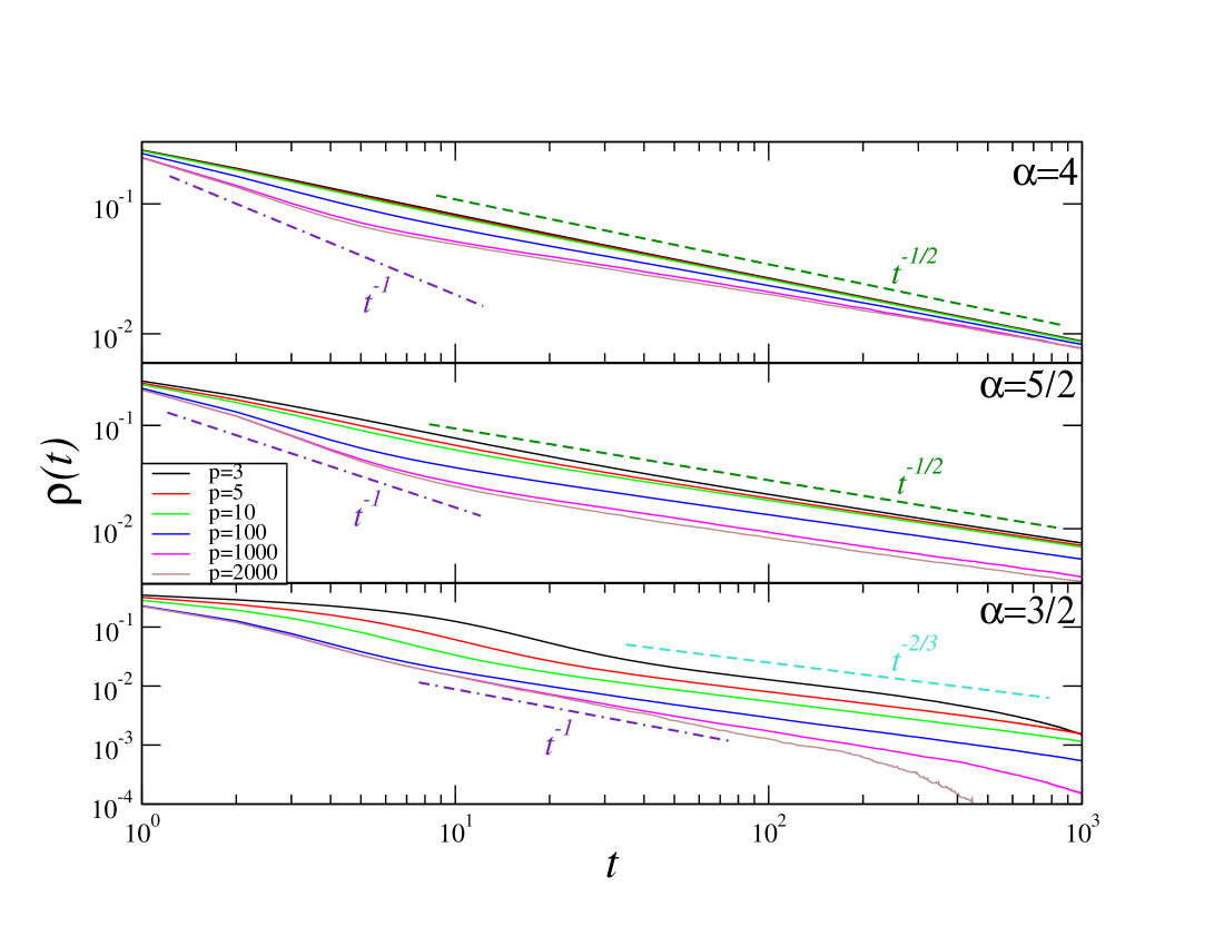
Figure 1: Time evolution of $\rho$, in a log-log plot, for $\alpha=4$ (top panel), $\alpha=5/2$ (central panel), and $\alpha=3/2$ (bottom panel). System size is $N=10^{3}$. In each panel, different curves refer to various values of $p$ (see legend). Dashed lines are the expected slopes ($t^{-1/2}$ and $t^{-2/3}$ for the IM (at $T\neq 0$), as reported in table 1.

Summarizing, the asymptotic behavior of the pVM falls in the universality class of the IM at small temperatures for any value of $p$, the effect of changing this parameter being only the extension of the pre-asymptotic stage where the universality class of the T=0 IM is temporarily observed. In view of the discussion contained in Sec. II, one toggles between the two behaviors crossing over from $p\ll N$ to $p\gtrsim N$. Hence it is natural to expect that physical quantities, specifically $\rho$, should not depend separately on $p$ and $N$, but only on the ratio. Then, reinstating the $N$ and $p$ dependence in the interfacial density $\rho(t;p,N)$, which we omitted before for simplicity, we should have

$$\rho(t;p,N)=R\left(t;\frac{p}{N}\right),$$ (16)

where $R(t;x)$ is a function with the following limiting behaviors

$$R(t;x)=\left\{\begin{array}[]{lr}t^{-a_{0}},&\hskip 28.45274pt\mbox{for }x\ll 1,\\ t^{-a_{T}},&\mbox{for }x\gtrsim 1,\end{array}\right.$$ (17)

where $a_{0}$ and $a_{T}$ indicate the asymptotic value of the $a$ exponent in the IM quenched to $T=0$ or to a small finite temperature $T$, respectively. Eq. (16) is meant for large times but before finite-size effects enter the game; in other words with the order of the limits $\lim_{t\to\infty}\lim_{N\to\infty}$.

We test this conjecture numerically in Fig. 2, for $\alpha=3/2$. In each of the three panel we plot $\rho$ for different values of $p$ and system sizes chosen as to have a fixed (within the same panel) value of $x=p/N$. The three panels correspond to $x=2,1,10^{-1}$, so to span all the crossover pattern described by Eq. (17). Firstly, since at fixed $x$ smaller values of $p$ correspond to smaller system sizes, we see that for smaller $p$ the finite size effects, signalled by the downward late-time bending of the curves, is observed before. This being said, looking at sufficiently large times (but before such finite-size effect) one sees that the curves superimpose (for any $x$), according to Eq. (16), and that the decay exponent $a$ matches $a_{0}=1$ for $x\gtrsim 1$ while it is is consistent with $a_{T}=2/3$ for $x\ll 1$, which is the content of Eq. (17). We found similar results for other values of $\alpha$, with $a$ toggling in any case between the corresponding values of $a_{0}$ and $a_{T}$.

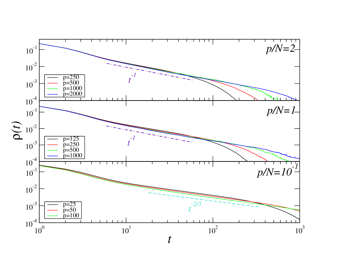
Figure 2: Time evolution of $\rho$, in a log-log plot for $\alpha=3/2$ and different values of $p$ (see legend) and system sizes $N$, chosen as to have a fixed value of $x=p/N$ in any case ($p/N=2,1,10^{-1}$ in the upper, central, and lower panel, respectively). Dashed lines are the expected slope $t^{-1}$ and $t^{-2/3}$ for the IM quenched to $T=0$ or to $T>0$, respectively.

IV.2 $\alpha\leq 1$

We have already discussed the fact that the IM with $\alpha\leq 1$, exhibits formation and coarsening of domains only in a fraction $P_{\alpha}$ of its dynamical realizations. The remaining cases are characterized by more homogeneous configurations where, after a microscopic time, all the spins take the same sign and $\rho$ vanishes. $P_{\alpha}$ decreases upon lowering $\alpha$ until $P_{\alpha}=0$ for $\alpha=0$, corresponding to the full mean-field situation. On the other hand, in the voter model a similar phenomenon is not observed and all the trajectories have, besides the intrinsic randomness, a qualitatively similar behavior as the metastable stationary state is approached, with a finite amount of interfaces present in the system. This is true until finite-size effects become relevant and consensus, namely a fully ordered state, is eventually achieved. The time of this occurrence, however, diverges with $N$ and hence full ordering is impossible in the thermodynamic limit. The first thing we have to address, therefore, is whether the pVM conforms to one of these two contrasting behaviors. Our simulations show that in the pVM interfaces are present at any time (clearly, still limiting to the time domain where the finite-size effects discussed above are absent). We arrived at this conclusion by computing the fraction $P_{\alpha}$ at time $t=1$. In the case $\alpha=0.95$, for instance, we found that domains where always found, i.e. $P_{\alpha}=1$ over the $5\cdot 10^{4}$ realizations considered.

In Corberi et al. (2023), considering the IM with $\alpha\leq 1$ quenched to $T\equiv 0$ and pruning only the configurations exhibiting coarsening, it was conjectured that $a=1$. However such hypothesis relies on poor numerical evidences, due to huge noise and important finite-size effects, and on an uncontrolled analytical approximation. On the contrary, nothing is known about $a$ for quenches to finite temperatures.

Our result for the density of interfaces in the pVM with $\alpha\leq 1$ are reported in Fig. 3. Data become progressively noisier as $\alpha$ is lowered because the longer ranged interactions give rise to a larger correlation among the spins making any kind of self-averaging less effective . The same feature is found in simulations of the IM with $\alpha\leq 1$ Corberi et al. (2021, 2023).

If a picture similar to the cases with $\alpha>1$ still applies now, we should expect to see the putative exponent $a=1$ at least for $p\to\infty$, where the pVM should match the universal behaviour of the IM at $T\equiv 0$, namely an exponent $a=1$. This is actually seen in the figure. Indeed, for $p=1000,2000$ and sufficiently long times ($t\gtrsim 10$) one sees a regime well consistent with $a=1$, before finite size effects bend downwards the curves around $t\simeq 10^{2}$. On the other hand, the behaviour of $\rho$ is very different when smaller values of $p$ are considered, in that a much faster decay is observed. In the interpretative scheme put forward insofar, this should correspond to the behaviour of the IM at $0<T<T_{c}$. However, since nothing is known about the IM at finite temperatures when $\alpha\leq 1$, we cannot comment further the behavior of these curves.

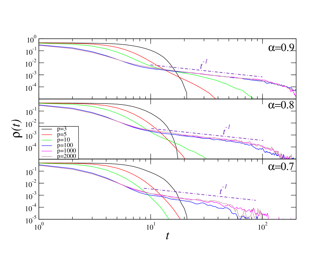
Figure 3: Time evolution of $\rho$, in a log-log plot, for $\alpha=0.9$ (top panel), $\alpha=0.8$ (central panel), and $\alpha=0.7$ (bottom panel). In each panel, different curves refer to various values of $p$ (see legend). Dashed lines are the slope with $a=1$ conjectured for the IM at $T\equiv 0$), as reported in table 1.

All the results presented insofar indicate that, for any value of $\alpha$, the pVM belongs to the IM universality class for any value of $p\geq p^{*}=3$. An heuristic understanding of that could be the following. According to the discussion of Sec. II (around Eq. (15)), the convergence of the pVM to the IM for $p\to\infty$ is due to fading off of fluctuations in the choice of the $p$ spins influencing the flipping candidate $S_{i}$, a sort of internal averaging. Lets stipulate that $\hat{p}(N)$ is a certain value of $p$ such that, for $p\geq\hat{p}$ the pVM can be regarded sufficiently near to the IM, given a reference tolerance, while it is not so for smaller $p$-values. Let us notice that, in order to have an effective averaging by choosing $p$ objects among $N$ it must be $p\sim N$ at least. Now, lets consider a slightly different model where each spin attempts a flip two consecutive times (so it can flip even twice, thus returning to its original state). In such double move, which can be regarded as the elementary move of this deformed dynamics, all the other spins are fixed. One can imagine that this different dynamical rule does not modify to much the long-time behavior. Upon evolving this model at $p=\hat{p}/2$ one could argue that the same level of internal averaging is obtained as the one present in the original model at $p=\hat{p}$, hence its resemblance to the IM would be still satisfactory. Generalizing this idea, we could think to a class of models where each elementary move is, in reality, made of $\kappa$ flip attempts. This way, the deformed kinetics at $p=\hat{p}/\kappa$ could be also sufficiently close to the one of the IM.

How large $\kappa$ can be chosen? Since we are interested in the behavior of the system on large timescales, and times are naturally measured in Montecarlo steps, where $N$ spins flips are attempted, we argue that, in order not to change the large-time behavior, it must be $\kappa/N\lesssim 1$. This mean that the smallest value $p^{*}$ that can be reached, under the condition of staying close enough to the IM, is of ${\cal O}(1)$. This heuristic argument shows that $p^{*}$ does not scale with $N$, however clearly it does not explain the precise value $p^{*}=3$ found in our studies. Let us remark, however that such value is smallest one where the non-linearity of $\sigma$ (see Eq. (7)) plays a role.

V Conclusions

In this paper we have considered the ordering kinetics of the pVM with algebraic long-range interactions. In this system individual spins $S_{i}$ flip according to a local field $H_{i}$ produced by the action of $p$ other agents selected randomly at distance $r$ with a probability decaying algebraically with $r$ (Eq. 2)). This ferromagnetic model reduces to the usual VM with long-range interactions for $p=1$, while it is expected to be equivalent to the IM for large $p$. For generic $p$ it can be considered as a kind of interpolation between the two. Our study shows that for $p=2$ the model can be mapped exactly on the usual VM (namely $p=1$), whereas for any other value of $p$ its properties, inferred by the asymptotic time-decay of the interface density $\rho$, fall into the universality class of the IM after a quench to a finite $T$. Moreover, a behavior in the universality class of the IM quenched to $T=0$ is observed preasymptotically in a time domain which diverges as $p\to\infty$. This is embodied by a scaling form (Eq. (16)) where $p$ and $N$ enter $\rho$ only through their ratio $x=p/N$. This can be rationalized by interpreting the random choice of the $p$ spins as a sort of effective temperature which is bound to vanish in the limit $p\to\infty$ due to the perfect averaging obtained in this way.

Our study can be framed into the more general context of the possible reduction of the degrees of freedom of a theory. In the specific case of the models considered here it offers the possibility to study the IM with long-range interactions by mean of the pVM with $p\geq 3$, offering the great numerical advantage of reducing the computational time from $\sim N^{2}$ to $\sim pN$. Moreover, although for $p\geq 3$ the pVM is not exactly solvable, approximate calculations could possibly be more accessible than in the IM.

As pointed out at the end of Sec. IV, the difference between the cases with $p=1,2$ and those with larger values of $p$ amounts to the fact that the theory cannot be linearized in the latter cases. This might suggest that the results found in this paper could not be confined to the one-dimensional case considered here, but hold in full generality. If this is true, our study might open the way to a more efficient study of the ordering kinetics of the IM with long-range interactions that, at variance with the $1d$ case, are scarcer. Let us mention, for instance, the recent observation Agrawal et al. (2021); Christiansen et al. (2021) of a new growth exponent in the phase-ordering of a two-dimensional system quenched to $T=0$.

References

- Jȩdrzejewski et al. (2015) A. Jȩdrzejewski, A. Chmiel, and K. Sznajd-Weron, Phys. Rev. E 92, 052105 (2015).
- Chmiel et al. (2018) A. Chmiel, T. Gradowski, and A. Krawiecki, International Journal of Modern Physics C 29, 1850041 (2018).
- Rodriguez et al. (2011) D. E. Rodriguez, M. A. Bab, and E. V. Albano, Phys. Rev. E 83, 011110 (2011).
- Corberi and Castellano (2023) F. Corberi and C. Castellano, (2023), arXiv:arXiv:2309.16517 [cond-mat.stat-mech] .
- Corberi and Smaldone (2023) F. Corberi and L. Smaldone, “Ordering kinetics of the two-dimensional voter model with long-range interactions,” (2023), arXiv:2312.00743 [cond-mat.stat-mech] .
- Corberi and Smaldone (2024) F. Corberi and L. Smaldone, “Aging properties of the voter model with long-range interactions,” (2024), arXiv:2402.11079 [cond-mat.stat-mech] .
- Aiudi et al. (2023) R. Aiudi, R. Burioni, and A. Vezzani, Phys. Rev. B 107, 224204 (2023).
- Bray (1994) A. Bray, Advances in Physics 43, 357 (1994), https://doi.org/10.1080/00018739400101505 .
- Corberi et al. (2010) F. Corberi, L. F. Cugliandolo, and H. Yoshino, arXiv: Statistical Mechanics (2010).
- Corberi et al. (2019a) F. Corberi, E. Lippiello, and P. Politi, Journal of Statistical Physics 176, 510 (2019a).
- Corberi et al. (2017) F. Corberi, E. Lippiello, and P. Politi, EPL (Europhysics Letters) 119, 26005 (2017).
- Christiansen et al. (2019a) H. Christiansen, S. Majumder, and W. Janke, Phys. Rev. E 99, R011301 (2019a).
- Corberi et al. (2021) F. Corberi, A. Iannone, M. Kumar, E. Lippiello, and P. Politi, SciPost Phys. 10, 109 (2021).
- Corberi et al. (2019b) F. Corberi, E. Lippiello, and P. Politi, Journal of Statistical Mechanics: Theory and Experiment 2019, 074002 (2019b).
- Agrawal et al. (2021) R. Agrawal, F. Corberi, E. Lippiello, P. Politi, and S. Puri, Phys. Rev. E 103, 012108 (2021).
- Bray and Rutenberg (1994a) A. J. Bray and A. D. Rutenberg, Phys. Rev. E 49, R27 (1994a).
- Rutenberg and Bray (1994a) A. D. Rutenberg and A. J. Bray, Phys. Rev. E 50, 1900 (1994a).
- Christiansen et al. (2019b) H. Christiansen, S. Majumder, and W. Janke, Phys. Rev. E 99, 011301 (2019b).
- ichi Amari (1993) S. ichi Amari, Neurocomputing 5, 185 (1993).
- Mignacco et al. (2020) F. Mignacco, F. Krzakala, P. Urbani, and L. Zdeborová, in Advances in Neural Information Processing Systems, Vol. 33, edited by H. Larochelle, M. Ranzato, R. Hadsell, M. Balcan, and H. Lin (Curran Associates, Inc., 2020) pp. 9540–9550.
- Mignacco et al. (2021) F. Mignacco, P. Urbani, and L. Zdeborová, Machine Learning: Science and Technology 2, 035029 (2021).
- Mignacco and Urbani (2022) F. Mignacco and P. Urbani, Journal of Statistical Mechanics: Theory and Experiment 2022, 083405 (2022).
- Angelini et al. (2023) M. C. Angelini, A. G. Cavaliere, R. Marino, and F. Ricci-Tersenghi, arXiv:2309.05337 (2023), https://doi.org/10.1016/0925-2312(93)90006-O.
- Note (1) In usual equilibrium critical phenomena, a single exponent does not determine alone a universality class. In non-equilibrium states the matter is more elusive. In the following, therefore, improper statements such as “the two models fall in the same universality class” will be used to indicate that they share the same exponent .
- Kimura (1953) M. Kimura, Annual Rep. Nat. Inst. Genetics, Japan 3, 62 (1953).
- Kimura and Weiss (1964) M. Kimura and G. H. Weiss, Genetics 49, 561 (1964).
- Malécot et al. (1970) G. Malécot, D. Yermanos, and K. M. R. Collection, The Mathematics of Heredity (W. H. Freeman, 1970).
- Clifford and Sudbury (1973) P. Clifford and A. Sudbury, Biometrika 60, 581 (1973).
- Holley and Liggett (1975) R. A. Holley and T. M. Liggett, The Annals of Probability 3, 643 (1975).
- Liggett (2004) T. Liggett, Interacting Particle Systems, Classics in Mathematics (Springer Berlin Heidelberg, 2004).
- Cox and Griffeath (1986) J. T. Cox and D. Griffeath, The Annals of Probability 14, 347 (1986).
- Scheucher and Spohn (1988) M. Scheucher and H. Spohn, Journal of Statistical Physics 53, 279 (1988).
- Krapivsky (1992) P. L. Krapivsky, Phys. Rev. A 45, 1067 (1992).
- Frachebourg and Krapivsky (1996) L. Frachebourg and P. L. Krapivsky, Phys. Rev. E 53, R3009 (1996).
- Ben-Naim et al. (1996) E. Ben-Naim, L. Frachebourg, and P. L. Krapivsky, Phys. Rev. E 53, 3078 (1996).
- Sood and Redner (2005) V. Sood and S. Redner, Phys. Rev. Lett. 94, 178701 (2005).
- Sood et al. (2008) V. Sood, T. Antal, and S. Redner, Phys. Rev. E 77, 041121 (2008).
- Castellano et al. (2009a) C. Castellano, S. Fortunato, and V. Loreto, Rev. Mod. Phys. 81, 591 (2009a).
- Zillio et al. (2005) T. Zillio, I. Volkov, J. R. Banavar, S. P. Hubbell, and A. Maritan, Phys. Rev. Lett. 95, 098101 (2005).
- Antal et al. (2006) T. Antal, S. Redner, and V. Sood, Phys. Rev. Lett. 96, 188104 (2006).
- Ghaffari and Stollenwerk (2012) P. Ghaffari and N. Stollenwerk, in Numerical Analysis and Applied Mathematics ICNAAM 2012: International Conference of Numerical Analysis and Applied Mathematics, American Institute of Physics Conference Series, Vol. 1479, edited by T. E. Simos, G. Psihoyios, C. Tsitouras, and Z. Anastassi (2012) pp. 1331–1334.
- Caridi et al. (2013) I. Caridi, F. Nemiña, J. P. Pinasco, and P. Schiaffino, Chaos, Solitons & Fractals 56, 216 (2013).
- Gastner et al. (2018) M. T. Gastner, B. Oborny, and M. Gulyás, Journal of Statistical Mechanics: Theory and Experiment 2018, 063401 (2018).
- Castellano et al. (2009b) C. Castellano, S. Fortunato, and V. Loreto, Rev. Mod. Phys. 81, 591 (2009b).
- Redner (2019) S. Redner, Comptes Rendus Physique 20, 275 (2019).
- Mobilia (2003) M. Mobilia, Phys. Rev. Lett. 91, 028701 (2003).
- Vazquez and Redner (2004) F. Vazquez and S. Redner, Journal of Physics A: Mathematical and General 37, 8479–8494 (2004).
- Mobilia and Georgiev (2005) M. Mobilia and I. T. Georgiev, Phys. Rev. E 71, 046102 (2005).
- Dall’Asta and Castellano (2007) L. Dall’Asta and C. Castellano, Europhysics Letters 77, 60005 (2007).
- Mobilia et al. (2007) M. Mobilia, A. Petersen, and S. Redner, Journal of Statistical Mechanics: Theory and Experiment 2007, P08029 (2007).
- Stark et al. (2008) H.-U. Stark, C. J. Tessone, and F. Schweitzer, Phys. Rev. Lett. 101, 018701 (2008).
- Castellano et al. (2009c) C. Castellano, M. A. Muñoz, and R. Pastor-Satorras, Physical Review E 80 (2009c), 10.1103/physreve.80.041129.
- Moretti et al. (2013) P. Moretti, S. Liu, C. Castellano, and R. Pastor-Satorras, Journal of Statistical Physics 151, 113 (2013).
- Caccioli et al. (2013) F. Caccioli, L. Dall’Asta, T. Galla, and T. Rogers, Physical Review E 87 (2013), 10.1103/physreve.87.052114.
- wien Hsu and wei Huang (2014) J. wien Hsu and D. wei Huang, Physica A: Statistical Mechanics and its Applications 416, 371 (2014).
- Khalil et al. (2018) N. Khalil, M. San Miguel, and R. Toral, Phys. Rev. E 97, 012310 (2018).
- Baron et al. (2022) J. W. Baron, A. F. Peralta, T. Galla, and R. Toral, Entropy 24, 1331 (2022), arXiv:2208.04264 [physics.soc-ph] .
- Castellano et al. (2009d) C. Castellano, M. A. Muñoz, and R. Pastor-Satorras, Phys. Rev. E 80, 041129 (2009d).
- Liu et al. (2013) S. Liu, C. Castellano, and R. Pastor-Satorras, Journal of Statistical Physics 151, 113 (2013).
- Nyczka et al. (2012) P. Nyczka, K. Sznajd-Weron, and J. Cisło, Phys. Rev. E 86, 011105 (2012).
- Bray and Rutenberg (1994b) A. J. Bray and A. D. Rutenberg, Phys. Rev. E 49, R27 (1994b).
- Rutenberg and Bray (1994b) A. D. Rutenberg and A. J. Bray, Phys. Rev. E 50, 1900 (1994b).
- Dyson (1969) F. J. Dyson, Communications in Mathematical Physics 12, 91 (1969).
- Corberi et al. (2023) F. Corberi, M. Kumar, E. Lippiello, and P. Politi, Chaos, Solitons & Fractals 173, 113681 (2023).
- Note (2) The curves with the larger values of are the results of a 6 month cpu time calculation on a standard processor.
- Christiansen et al. (2021) H. Christiansen, S. Majumder, and W. Janke, Phys. Rev. E 103, 052122 (2021).