Sparse Global Matching for Video Frame Interpolation with Large Motion

Abstract

Large motion poses a critical challenge in Video Frame Interpolation (VFI) task. Existing methods are often constrained by limited receptive fields, resulting in sub-optimal performance when handling scenarios with large motion. In this paper, we introduce a new pipeline for VFI, which can effectively integrate global-level information to alleviate issues associated with large motion. Specifically, we first estimate a pair of initial intermediate flows using a high-resolution feature map for extracting local details. Then, we incorporate a sparse global matching branch to compensate for flow estimation, which consists of identifying flaws in initial flows and generating sparse flow compensation with a global receptive field. Finally, we adaptively merge the initial flow estimation with global flow compensation, yielding a more accurate intermediate flow. To evaluate the effectiveness of our method in handling large motion, we carefully curate a more challenging subset from commonly used benchmarks. Our method demonstrates the state-of-the-art performance on these VFI subsets with large motion.

1 Introduction

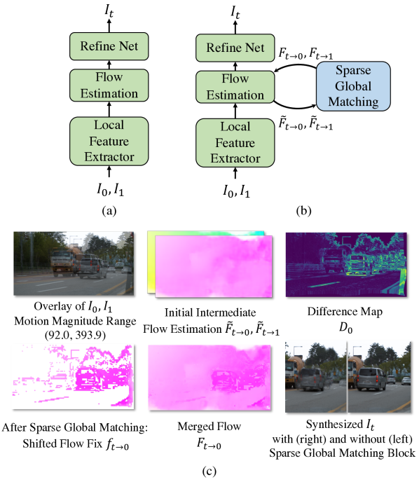
Figure 1: (a) Our framework without sparse global matching, pretrained on small motion dataset, for capturing local details. (b) Our framework with sparse global matching, fine-tuned on large motion dataset, for capturing global large motion. (c) Key components in our algorithm, illustrating the effect of our sparse global matching branch. (Using Ours-1/4-Points, from Table 1.)

Video Frame Interpolation (VFI) seeks to generate the intermediate frame from a given pair of inference frames, which has received increasing attention. It has various real-life applications, such as creating slow motion videos [13, 10, 3], video compression [12, 33] and novel view synthesis [1, 7, 38]. Currently, flow-based algorithms occupy a prominent position [37, 9, 26, 28, 17, 18, 30] in VFI task, where the flow from the target frame to the input frames, namely, intermediate flow, is explicitly estimated for warping input frames to the target frame.

Nevertheless, existing optical flow [32, 34, 11] algorithms cannot be directly applied to estimate intermediate flows due to the absence of the target frame. To address this, many algorithms first estimate the bidirectional flow between two input frames and then generate intermediate optical flows using various flow reversal techniques [35, 19, 13, 29, 24, 39, 15]. Alternatively, recent algorithms directly estimate the intermediate flow with proper supervision [17, 37, 9] and achieve improved performance on datasets where small-to-medium motions are prevalent [27].

However, real-world video frame interpolation encounters various complex challenges, with the problem of handling large motion being particularly prominent. In scenarios characterized by large motion, the correspondence of objects between frames is hard to locate due to the large pixel shifting. Many works have been proposed to alleviate this problem. For example, XVFI [29] addressed this by creating an extreme 4K training dataset and a scalable framework. However, its performance improvement is limited when applied to small motion scenarios [25]. FILM [27] introduced scale-agnostic features and a weight-sharing approach to improve model generalization across different motion scales. In fact, due to its limited receptive field, the model’s depth can become excessively deep when dealing with large motion. This increases computational complexity and falls short in handling fast-moving small objects.

In this paper, we introduce a sparse global matching pipeline to specifically handle the challenges posed by large motion in the VFI task, by effectively integrating global-level information into intermediate flow estimation. Our VFI method establishes sparse global correspondences between input frames using a global receptive field and takes a two-step strategy to compensate for the intermediate flow estimation. Specifically, as shown in Figure 1 (a - b), our method begins with an initial estimation of a pair of intermediate flows using a relatively high-resolution feature map. Following this initial estimation, our approach incorporates a sparse global matching branch to locate potential error in the flow estimation results, and then produce flow residual to provide an effective remedy for capturing large motion.

To be specific, in our sparse global matching branch, we build a difference map to pinpoint the flaws in initial intermediate flow estimations. Concentrating on these defective areas, our approach employs sparse global matching to establish global correspondences between two adjacent input frames, specifically at these sparsely targeted locations. Subsequently, we convert this bidirectional sparse flow correspondence into intermediate flow compensation. Finally, we employ a flow merging block to adaptively merge the initial intermediate flows and flow compensation, thereby effectively combining the local details with the global correlation. As shown in Figure 1 (c), our sparse global matching branch can effectively locate the error regions and rectify the flaws in the initial intermediate flow estimation, yielding a significantly enhanced synthesized intermediate frame.

In order to benchmark the effectiveness of our sparse global matching module on handling large motion, we carefully analyze motion magnitude and sufficiency within existing benchmarks, X-Test [29], Xiph [22] and SNU-FILM [4]. In our analysis, we utilize the motion sufficiency filtering method described in [1], emphasizing the minimum of the top 5% of each pixel’s flow magnitude as the key indicator of large motion sufficiency. In the end, we carefully curate the most challenging subsets for large motion frame interpolation evaluation. In the most challenging testing conditions, our proposed method demonstrates a substantial improvement in terms of PSNR, enhancing it by $0.66$ dB while correcting half of the points in initial flow estimation. Furthermore, even with the correction of just $1/8$ points, we still observe a notable increase of $0.48$ dB. Notably, our approach establishes a new state-of-the-art performance benchmark in these exceptionally challenging scenarios. In summary, our main contributions include:

• We introduce a sparse global matching algorithm tailored to effectively capture large motion.

• We designed an effective two-step framework for capturing large motion. First, by estimating initial intermediate flows to extract the local details, then targets and corrects the detected flaws through sparse global matching at sparsely targeted defective points.

• Our models demonstrate state-of-the-art performance on the most challenging subset of the commonly used large motion benchmark, namely, X-Test-L, Xiph-L, SNU-FILM-L hard and extreme.

2 Related Work

Figure 2: Overview of our proposed structure. First, local features are extracted by a local feature extractor for flow estimation $\widetilde{F}_{t\rightarrow 0},\widetilde{F}_{t\rightarrow 1}$. Then, our sparse global matching branch locates the flaws by constructing difference maps $D_{0},D_{1}$. Next, we perform sparse global matching using global features extracted by a global feature extractor. Finally, after shifting global correspondences $f_{0\rightarrow 1},f_{1\rightarrow 0}$ to intermediate flow compensation $f_{t\rightarrow 1},f_{t\rightarrow 0}$, we adaptively merge $\widetilde{F}_{t\rightarrow 0},\widetilde{F}_{t\rightarrow 1}$ with $f_{t\rightarrow 1},f_{t\rightarrow 0}$ and adopts a flow refine in a residual manner for interpolating the intermediate frame.

2.1 Flow-Based Video Frame Interpolation

Flow-based algorithms for video frame interpolation focus on estimating intermediate flows. These flows enable the model to either forward warp or backward warp the input frames to the target frame. Some algorithms first compute bidirectional flows between two input frames and apply different flow reversal techniques to obtain intermediate flows [24, 35, 29], while the others directly estimate intermediate flows [9, 37, 17].

However, flow reversal techniques may introduce artifacts to intermediate flows, which can harm the details of the intermediate flows, causing misalignment [13] or holes [35]. Direct estimation of intermediate flows is also restricted by the model design, usually has a limited perceptive field [9, 37], and lacks robustness on large motion.

Addressing the issue of large motion in video frame interpolation, FILM [27] adopts a coarse-to-fine approach and shares weights between layers. It also trains on data with varied motion magnitudes, enabling it to learn to handle large motions. AMT [18] uses the RAFT-like structure to construct an all-pair correlation map and locally refines the intermediate flow afterward. BiFormer [26] employs a global feature extractor to extract global features and build local bilateral correlation maps. However, due to the high resolution of the VFI task, giving the model a genuine global receptive field is challenging.

In contrast, our work uses local features to estimate the intermediate flows and global features to sparsely generate bidirectional flow compensation by global matching. We then adaptively merge the flows and flow compensation to obtain the final intermediate flow with both global information and local details.

2.2 Transformer

Transformers have gained widespread popularity across various computer vision tasks [6, 20, 2, 40], demonstrating impressive feature extraction capabilities. Recently, Transformer-based backbone has already been introduced to solve VFI task [22, 16, 28, 37]. VFIFormer [21] uses cross-scale window-based attention. EMA-VFI [37] uses Inter-frame Attention to extract appearance and motion features using the same similarity matrix. BiFormer [26] adopts pretrained Twins architecture [5] for global feature extraction and builds local bilateral correlation cost volume. However, when handling large motion, these methods are more or less restricted by their local receptive field. Therefore, we propose a two-step strategy: employing a hybrid Transformer and CNN-based backbone for initial flow estimation, followed by a sparse global matching block utilizing a global receptive field.

2.3 Global Matching

Global matching is extensively studied in local feature matching tasks. LoFTR [31] replaces the traditional dense matching method, using cost volume to search for correspondence, with self and cross attention layers in Transformer. COTR [14] takes a different approach by formulating the correspondence problem as a functional mapping and utilizing a Transformer as the function to query the points of interest. For dense matching, GMFlow [34] adopted Transformer block to extract strong discriminative features to build a global matching map. In VFI tasks, not every part of the image requires dense global matching. Our sparse global matching strategy, on the other hand, specifically targets and corrects the defective areas of the flows.

3 Method

Given a pair of RGB frames $I_{0}$, $I_{1}$, and a timestep $t$, we need to synthesize an intermediate frame $I_{t}$. We illustrate our overall model pipeline in Figure 2.

Our method consists of a local feature branch and a sparse global matching branch. The local feature branch is responsible for estimating the initial intermediate flows, namely $\widetilde{F}_{t\rightarrow 0}$ and $\widetilde{F}_{t\rightarrow 1}$. In the sparse global matching branch, we focus on the defective areas of $\widetilde{F}_{t\rightarrow 0}$, $\widetilde{F}_{t\rightarrow 1}$, and perform sparse global matching to obtain flow compensation, $f_{t\rightarrow 0}$ and $f_{t\rightarrow 1}$. Then we adaptively merge $\widetilde{F}_{t\rightarrow 0}$ and $\widetilde{F}_{t\rightarrow 1}$ with $f_{t\rightarrow 0}$ and $f_{t\rightarrow 1}$ by our flow merge block, to obtain more accurate intermediate flows, $F_{t\rightarrow 0}$, $F_{t\rightarrow 1}$. Finally, after a few flow refine blocks, we use this pair of intermediate flows to synthesize the intermediate frame $\widehat{I_{t}}$.

In the following, we first introduce each component in our local feature branch briefly in Section 3.1. From Section 3.2 and onward, we delve into a detailed discussion of our sparse global matching branch.

3.1 Local Feature Branch

As shown in Figure 2, our local feature branch consists of three parts, namely, the local feature extractor, the flow estimation block, and the RefineNet [9]. We draw inspiration from RIFE [9] and EMA-VFI [37], while retaining certain distinctive aspects. We now introduce them sequentially.

Local Feature Extractor. EMA-VFI [37] has already verified the effectness of CNN and Transformer hybrid structure. We follow its design and keep our deepest feature resolution stays at $H/8\times W/8$ scale, instead of $H/16\times W/16$ in EMA-VFI. Furthermore, we simplified the specially designed Transformer structure in EMA-VFI to simple cross attention to extract inter-frame appearance features at a lower computation cost.

Flow Estimation. We use the extracted appearance feature and input frames $I_{0},I_{1}\in\mathbb{R}^{3\times H\times W}$ to directly estimate intermediate flows $F_{t\rightarrow 0}$, $F_{t\rightarrow 1}$, along with a fusion map $O$, in a coarse-to-fine manner. This is achieved by several layers of CNN block, inspired by the intuitive design of RIFE [9] and EMA-VFI [37]. Then, the target frame can be generated by:

$$\widehat{I}_{t}=O\odot\overleftarrow{\mathcal{W}}\left(I_{0},F_{t\rightarrow 0}\right)+(1-O)\odot\overleftarrow{\mathcal{W}}\left(I_{1},F_{t\rightarrow 1}\right),$$ (1)

where $\overleftarrow{\mathcal{W}}$ is image backward warping operation, $\odot$ is Hadamard product operator.

Flow Refine. We share the same U-net-shaped network with RIFE to refine the synthesized frame $\widehat{I}_{t}$. More details can be found in Appendix A.

3.2 Locate Flaws in Flows: Difference Map

Due to the limited receptive field of local feature branch, the estimated initial bidirectional flows, $\widetilde{F}_{t\rightarrow 0}$ and $\widetilde{F}_{t\rightarrow 1}$, may be relatively coarse. Consequently, it is necessary to identify the flaws in $\widetilde{F}_{t\rightarrow 0}$ and $\widetilde{F}_{t\rightarrow 1}$. Therefore, we construct the difference map $D_{0}$ and $D_{1}$ to check the correctness of $\widetilde{F}_{t\rightarrow 0}$ and $\widetilde{F}_{t\rightarrow 1}$, by using both of the input frames $I_{0}$ and $I_{1}$ as ground truth reference. The values in the difference maps $D_{0}$ and $D_{1}$ serve as indicators of the likelihood of error in flow estimation, with higher values suggesting a greater probability of inaccuracies.

In particular, we first use $\widetilde{F}_{t\rightarrow 0}$ to backward warp $I_{0}$ to $\widetilde{I}_{t}$, then use $\widetilde{F}_{t\rightarrow 1}$ to forward warp $\widetilde{I}_{t}$ to $\widetilde{I}_{1}$. And we compare the $\widetilde{I}_{1}$ and input frame $I_{1}$ by doing summation over RGB channels after subtraction to obtain difference map $\widetilde{D}_{0\rightarrow 1}$.

$$\widetilde{I}_{1} =\overrightarrow{\mathcal{W}}\left(\overleftarrow{\mathcal{W}}\left(I_{0},\widetilde{F}_{t\rightarrow 0}\right),\widetilde{F}_{t\rightarrow 1}\right),$$ (2)

$$\widetilde{D}_{0\rightarrow 1} =\sum_{RGB}|I_{1}-\widetilde{I}_{1}|,$$ (3)

where $\overleftarrow{\mathcal{W}}$ is backward warp, $\overrightarrow{\mathcal{W}}$ is forward warp.

Through the combination of backward warp and forward warp, we get an initial difference map $\widetilde{D}_{0\rightarrow 1}$. Currently, the flaws in $\widetilde{D}_{0\rightarrow 1}$ are caused by two reasons, the first reason is due to the flaws in our coarse flow estimation, $\widetilde{F}_{t\rightarrow 0}$, $\widetilde{F}_{t\rightarrow 1}$. The second reason is that even if $\widetilde{F}_{t\rightarrow 0}$, $\widetilde{F}_{t\rightarrow 1}$ were perfectly accurate, occlusions and cropping would still occur inevitably, i.e. some existing pixels in $I_{0}$ disappearing in $I_{1}$, creating incorrect pixel mappings and holes in the warped image.

To filter out the second cause of flaws, we create a map full of ones, and repeat the above warping process to obtain a $0/1$ mask, $M_{0\rightarrow 1}^{holes}$. The positions in mask $M_{0\rightarrow 1}^{holes}$ where the element becomes 0 correspond to the potential hole areas in the warped image $\widetilde{I}_{1}$.

Then, we can multiply this map $M_{0\rightarrow 1}^{holes}$ with our initial difference map $\widetilde{D}_{0\rightarrow 1}$ to filter out the potential holes caused by occlusion and cropping, and obtain $D_{0\rightarrow 1}$, focusing on the flaws caused by inaccurate intermediate flow estimation.

$$D_{0\rightarrow 1}=M_{0\rightarrow 1}^{holes}\odot\widetilde{D}_{0\rightarrow 1}.$$ (4)

As a result, $D_{0\rightarrow 1}$ enables us to identify the misaligned regions in $\widetilde{I}_{1}$ that are caused solely by the flaws in the estimated flows $\widetilde{F}_{t\rightarrow 0}$, $\widetilde{F}_{t\rightarrow 1}$. Furthermore, we reverse the previous warping combination to find the underlying source points responsible for these misalignments in $\widetilde{I}_{1}$.

$$D_{0}=\overrightarrow{\mathcal{W}}\left(\overleftarrow{\mathcal{W}}\left(D_{0\rightarrow 1},\widetilde{F}_{t\rightarrow 1}\right),\widetilde{F}_{t\rightarrow 0}\right).$$ (5)

Difference map $D_{0}$ illustrates the extent to which each point in $I_{0}$ leads to the misalignment in $\widetilde{I}_{1}$. To address this, it is essential to prioritize the regions with higher values in $D_{0}$. These regions indicate the points that exacerbate significant misalignment. Difference map $D_{1}$ can be produced symmetrically.

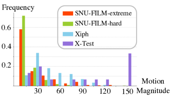
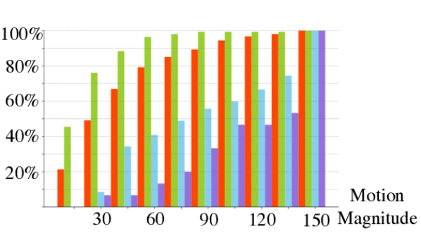
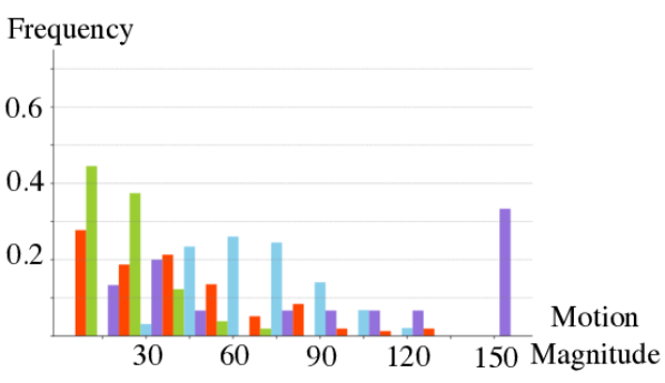
(a) Mean Motion Magnitude

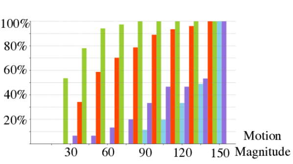
(b) Motion Sufficiency Ranking

Figure 3: Large motion dataset benchmark analysis. Top: Whole dataset. Below: Keeping the most challenging half of Xiph and SNU-FILM. Four charts share the same legend.

3.3 Sparse Global Matching

To emphasize the region with higher values in $D_{0}$ and $D_{1}$, we can select the top-$k$ points out of $D_{0}$, $D_{1}$ and do global matching for those points to provide more accurate matching flow $f_{0\rightarrow 1}$ and $f_{1\rightarrow 0}$, for preparing the flow compensation $f_{t\rightarrow 1}$ and $f_{t\rightarrow 1}$.

Sparse global matching allows the selected points in $I_{0}$ to have a global receptive field on $I_{1}$. We adopt the pretrained global feature extractor from GMFlow [34] to generate discriminative global features $A_{0}^{i},A_{1}^{i}\in\mathbb{R}^{\left(\frac{H}{2^{i}}\cdot\frac{W}{2^{i}}\right)\times C}$, where C is the number of feature channels. We construct a sparse feature map $a_{0}^{i}\in\mathbb{R}^{K\times C}$ according to top-$k$ indices selected from $D_{0}$. The corresponding area of $A_{0}^{i},A_{1}^{i}$ should have higher similarity, and the same intuition also applies to $a_{0}^{i}$ and $A_{1}^{i}$. Therefore, we can construct a similarity matrix $S_{0\rightarrow 1}\in K\times\left(\frac{H}{2^{i}}\cdot\frac{W}{2^{i}}\right)$:

$$S_{0\rightarrow 1}=\it Softmax\left(\frac{a_{0}^{i}A_{1}^{i}}{\sqrt{C}}\right).$$ (6)

Then we create a coordinate map $B\in\mathbb{R}^{\left(\frac{H}{2^{i}}\cdot\frac{W}{2^{i}}\right)\times 2}$. Using top-$k$ indices selected from $D_{0}$, we extract the corresponding points from the coordinate map $B$ to form a sparse coordinate map $b_{0}\in\mathbb{R}^{K\times 2}$. We use the product between similarity matrix $S_{0\rightarrow 1}$ and $b_{0}$ to represent the estimated position in $I_{1}$ for selected $k$ points. Therefore, the subtraction between the previous product $S_{0\rightarrow 1}b_{0}$ and $b_{0}$ can represent the flow for those points, namely $f_{0\rightarrow 1}$:

$$\widetilde{f}_{0\rightarrow 1}=S_{0\rightarrow 1}b_{0}-b_{0}.$$ (7)

Thus, $\widetilde{f}_{0\rightarrow 1}$ is obtained in a global matching manner, making it more capable of capturing large motions. Finally, we reuse the top-$k$ indices from $D_{0}$ to fill $\widetilde{f}_{0\rightarrow 1}\in\mathbb{R}^{K\times 2}$ to $f_{0\rightarrow 1}\in\mathbb{R}^{\frac{H}{2^{i}}\times\frac{W}{2^{i}}\times 2}$ with zero. $f_{1\rightarrow 0}$ can be obtained symmetrically.

3.4 Flow Shifting

The goal of our sparse global matching branch is to acquire sparse flow compensation $f_{t\rightarrow 0}$ and $f_{t\rightarrow 1}$ to improve the estimated intermediate flows, $\widetilde{F}_{t\rightarrow 0}$, $\widetilde{F}_{t\rightarrow 1}$, with large motion capturing ability. Next, we shift $f_{0\rightarrow 1}$, $f_{1\rightarrow 0}$ to $f_{t\rightarrow 1}$, $f_{t\rightarrow 0}$ by flow shifting, which can help mitigate the coordinate system mismatch.

We intercept a $(1-t)$ proportion of $f_{0\rightarrow 1}$ and shift this $(1-t)$ proportion along the remaining $t$ proportion of the flow $f_{0\rightarrow 1}$. Through this shifting operation, we can obtain $f_{t\rightarrow 1}$, and the shifting operation is performed by forward warping:

$$f_{t\rightarrow 1}=\overrightarrow{\mathcal{W}}\left((1-t)f_{0\rightarrow 1},tf_{0\rightarrow 1}\right),$$ (8)

$$f_{t\rightarrow 0}=\overrightarrow{\mathcal{W}}\left(tf_{1\rightarrow 0},(1-t)f_{1\rightarrow 0}\right).$$ (9)

Note that $f_{t\rightarrow 1}$ is flow shifted by $f_{0\rightarrow 1}$ and $f_{t\rightarrow 0}$ is flow shifted by $f_{1\rightarrow 0}$, we also list the $f_{t\rightarrow 0}$ in Equation 9 for clarity.

After the forward warping process, the number of sparsely chosen points will potentially change, and we will again choose the top-$k$ points with the least occlusion possibility.

Instead of using the estimated target frame $\widetilde{I}_{t}$ and input frames $I_{0}$, $I_{1}$ to perform global matching and obtain intermediate flow compensation $f_{t\rightarrow 0}$ and $f_{t\rightarrow 1}$, we use global matching between $I_{0}$, $I_{1}$ only and perform flow shift. The reason is that $\widetilde{I}_{t}$ synthesized by $\widetilde{F}_{t\rightarrow 0}$ and $\widetilde{F}_{t\rightarrow 1}$ is not reliable. Since we aim to minimize accumulated propagation errors, we endeavor to minimize the usage of intermediate results wherever possible.

3.5 Flow Merge Block

If we directly replace $\widetilde{F}_{t\rightarrow 0}$ and $\widetilde{F}_{t\rightarrow 1}$ with the flow compensation $f_{t\rightarrow 0}$ and $f_{t\rightarrow 1}$, the resulting flow may lack smoothness. In addition, the flow compensation $f_{t\rightarrow 0}$ and $f_{t\rightarrow 1}$ can also make mistakes. Therefore, we designed a flow merge block $\mathcal{M}$ to adaptively merge $\widetilde{F}_{t\rightarrow 0}$ and $f_{t\rightarrow 0}$, as well as $\widetilde{F}_{t\rightarrow 1}$ and $f_{t\rightarrow 1}$:

$$\widehat{F}_{t\rightarrow 0}=\mathcal{M}(\widetilde{F}_{t\rightarrow 0},f_{t\rightarrow 0}),$$ (10)

$$\widehat{F}_{t\rightarrow 1}=\mathcal{M}(\widetilde{F}_{t\rightarrow 1},f_{t\rightarrow 1}).$$ (11)

Inspired by the convex sampling in RAFT [32], we take the $\widehat{F}_{t\rightarrow 0}$ at each pixel to be the convex combination of $R\times R$ neighbors of $\widetilde{F}_{t\rightarrow 0}$ and $R\times R$ neighbors of $f_{t\rightarrow 0}$, where R is the neighborhood range. We use two convolutional layers to predict a $2\times R^{2}\times\frac{H}{2^{i}}\times\frac{W}{2^{i}}$ weight assignment, and apply softmax of the $2\times R^{2}$ neighborhood to obtain masks $\left[W_{main},W_{sgm}\right]$, where $W_{main},W_{sgm}\in\mathbb{R}^{R^{2}\times\frac{H}{2^{i}}\times\frac{W}{2^{i}}}$. $W_{main}$ stands for the weight for the local feature branch flow estimations, and $W_{sgm}$ stands for the weight for sparse global matching block flow compensation. Finally, the flow merge block outputs the $\widehat{F}_{t\rightarrow 0}$, obtained by taking weighted sum over the $\widetilde{F}_{t\rightarrow 0}$ and $f_{t\rightarrow 0}$ neighborhood.

4 Large Motion VFI Benchmark

To better illustrate our algorithm’s effectiveness in handling large motions, we analyzed several widely used large motion datasets, namely, SNU-FILM extreme and hard [4], Xiph [22], and X-Test [29]. We utilized RAFT [32] to estimate optical flow between input frames as evidence, allowing for a detailed assessment of motion magnitudes.

According to Figure 3(a), SNU-FILM and Xiph’s mean motion magnitude is much lower than X-Test’s. For example, we can see that about $60\%$ of SNU-FILM test cases’ mean motion magnitude is below 15, while Xiph has about $40\%$ test cases below 30.

In addition, we also refer to the criterion in [1] for assessing motion sufficiency, requiring at least 10% of each pixel’s flow to have a magnitude of at least 8 pixels within a $270\times 270$ resolution. We adjusted this criterion by lowering the percentage threshold to 5% while simultaneously increasing the required magnitude to account for the larger resolution of our input frames. This adjusted criterion, representing the minimum magnitude of the top 5% pixel flows, forms the basis for our proportion ranking of the benchmark datasets in Figure 3(b).

As depicted in the cumulative distribution chart Figure 3(b), we found that over 50% of X-Test have at least 5% of each pixel’s flow with a magnitude of at least 150 pixels. In contrast, Xiph  [22] and SNU-FILM  [4] contain fewer large motion pixels. Consequently, we focused our evaluation on the most challenging half of these benchmarks to assess our algorithm’s performance improvements in handling genuinely large motion data, with details in Section 5.2.

5 Experiments

Table 1: Quantitative evaluation (PSNR/SSIM) among different challenging benchmarks (see Section 4). The best results and the second best results in each column are marked in red and blue respectively. Ours-1/N Points means that we sparsely select 1/N points of the initial intermediate flows estimation to perform global matching by the evidence provided by difference map $D_{0},D_{1}$. “OOM” denotes the out-of-memory issue when evaluating on an NVIDIA V100-32G GPU.

	X-Test-L		SNU-FILM-L		Xiph-L
	2K	4K	hard	extreme	2K	4K
XVFI [29]	29.82/0.8951	29.02/0.8866	27.58/0.9095	22.99/0.8260	29.17/0.8449	28.09/0.7889
FILM [27]	30.08/0.8941	OOM	28.35/0.9156	23.06/0.8247	29.89/0.8533	27.11/0.7699
BiFormer [26]	30.32/0.9067	30.11/ 0.9070	28.18/0.9154	23.55/0.8383	29.61/0.8541	28.89/0.8133
RIFE [9]	29.87/0.8805	28.98/0.8756	28.19/0.9172	22.84/0.8230	30.18/0.8633	28.07/0.7982
EMA-VFI-small [37]	29.51/0.8775	28.60/0.8733	28.57/0.9189	23.18/0.8292	30.54/0.8718	28.40/0.8109
Ours-local-branch	30.39/0.8946	29.25/0.8861	28.73/0.9207	23.19/0.8301	30.89/0.8745	28.59/0.8115
Ours-1/8-Points	30.83/0.9022	29.73/0.8928	28.82/0.9208	23.54/0.8355	30.88/0.8749	28.90/0.8151
Ours-1/4-Points	30.88/ 0.9043	29.78/0.8948	28.86/ 0.9212	23.58/ 0.8368	30.89/ 0.8751	29.15/ 0.8169
Ours-1/2-Points	30.99/ 0.9072	29.91/ 0.8972	28.88/0.9216	23.62/0.8377	30.93/0.8755	29.25/ 0.8180

5.1 Implementation Detail

Training Datasets. We use two training datasets, Vimeo90K [36] for pretraining on small-to-medium motion and X4K1000FPS (X-Train) [29] for finetuning on large motion. Vimeo90K contains 51,312 triplets with a resolution of 448x256 for training. It has an average motion magnitude between 1 to 8 pixels [36]. X4K1000FPS (X-Train) contains 4,408 clips with a resolution of 768x768, each clip has 65 consecutive frames.

Local Feature Branch Training. We first train our model framework without the sparse global matching branch on Vimeo90K. We crop each training instance to 256x256 patches and perform random flip, time reversal, and random rotation augmentation, following  [37, 9]. The training batch size is set to 32. We use AdamW as our optimizer with $\beta_{1}=0.9$, $\beta_{2}=0.999$ and weight decay $1e^{-4}$. After 2,000 warmup steps, we gradually increase the learning rate to $2e^{-4}$, then use cosine annealing for 480k steps (300 epochs) to reduce the learning rate from $2e^{-4}$ to $2e^{-5}$. We follow the training loss design of  [37, 9] for both training and finetuning, which is included in Appendix B.

Sparse Global Branch Finetuning. We load our pretrained framework, and a global feature extractor from GMFlow [34], operating on $i=3$ in Equation 6. Then we integrate our sparse global matching branch into the framework, setting the sparsity ratio, i.e. 1/8, 1/4, 1/2, and finetuning the sparse global matching block on X-Train. When fine-tuning, we freeze the pretrained framework and the global feature extractor. We crop $512\times 512$ patches from the original training image, and random resize the input images with 50% probability to remain the $512\times 512$ size, 25% probability to downscale to $256\times 256$ size and 25% probability to $128\times 128$ size. We apply random flipping augmentation, following [29]. The batch size, learning rate and optimizer are the same as our local feature branch, except that warmup steps are set to 1k steps, and the total steps are set to 13.7k (100 epochs). The parameter freezing and random rescaling are for preserving the model’s ability to capture small motion details to the greatest extent possible.

5.2 Test Dataset

The proposed algorithm is designed for capturing large motions. Therefore, we test our model’s performance on the most challenging subset of the commonly used large motion benchmark, described in Section 4. We used PSNR (Peak Signal-to-Noise Ratio) and SSIM (Structural Similarity Index) as evaluation metric.

X4K1000FPS (X-Test) [29] is a 4K resolution benchmark, with 1000fps high frame rate. X-Test contains 15 clips of 33 successive 4K frames extracted from videos with 1000fps. We have selected X-Test, specifically with the largest temporal gap, naming X-Test-L, as our primary benchmark for evaluating large motion scenarios. We choose the $0_{th}$ and $32_{nd}$ frames as input and evaluate the quality of the synthesized $16_{th}$ output frame. Our testing procedure follows  [8] to provide both 4K and downsampled 2K resolution results.

SNU-FILM [4] is a widely-used VFI benchmark, with 1280x720 resolution. It has four different difficulty settings according to the temporal gap between two input frames, each with 310 triplets for evaluation. The larger the temporal gap, the more challenging this benchmark becomes. We test our model on the most challenging half of the SNU-FILM hard and extreme, naming SNU-FILM-L, with 155 triplets each. In the meantime, we also provide the performance on the ‘easy’ and ‘medium’ settings on the whole dataset in Table 2 to show our model’s capability in handling small-to-medium motions.

Xiph [22] is a 4K dataset with 8 scenes, each with 100 consecutive frames, extracted from 60fps videos. While it is often denoted as a benchmark for evaluating large motion, it does not match the level of difficulty exhibited by the X-Test. Therefore, we build this benchmark by doubling the input temporal gap and keeping the most challenging half of the dataset, naming Xiph-L, resulting in 192 test instances. By downsampling and center-cropping, we obtain ‘Xiph-L-2K’ and ‘Xiph-L-4K’ results, following  [23].

5.3 Comparison with Previous Methods

To fully inspect our model’s capacity on large motion, we evaluate our model on the aforementioned large motion datasets benchmarks and give our analysis compared results with recent VFI approaches, including ones designed for large motion, such as XVFI [29], FILM [27], BiFormer [26], and ones that performed well on commonly used datasets but not designed for large motion, namely, RIFE [9], EMA-VFI [37].

As shown in Table 1, the performance of our local feature branch, without finetuned on X-Train, has already surpassed most methods. We attribute this to the capacity of CNN and Transformer hybrid framework and high feature resolution ($H/8\times W/8$). But without the sparse global matching block, our results are not comparable to BiFormer in SNU-FILM-L extreme, Xiph-L-4K and XVFI in X-Test-L-4K.

After we incorporate the sparse global matching branch and finetuned on X-Train, our performance on large motion benchmarks are boosted. When we only sparsely select 1/8 of the points in initial flow estimation by the guidance of difference map $D_{0},D_{1}$, our performance improved 0.44dB on X-Test-L-2K and 0.48dB on X-Test-L-4K in terms of PSNR. With more points introduced to be compensated, the performance can be potentially improved by 0.6dB and 0.66dB on X-Test-L-2K and X-Test-L-4K respectively.

Small-to-medium Motion Benchmark Performance. From the data presented in Table 2, we observe that our results remain consistent with those in small-to-medium scenarios, and they are comparable to a SOTA algorithm, VFIFormer [21], on these benchmarks. This suggests that our local feature branch already achieves satisfactory results, and introducing our sparse global matching branch has a limited negative impact on the overall performance.

Table 2: Performance on small-to-medium benchmarks, SNU-FILM easy and medium.

	SNU-FILM
	easy		medium
	PSNR	SSIM	PSNR	SSIM
VFIFormer [21]	40.13	0.9907	36.09	0.9799
Local Branch (ft.)	40.15	0.9907	36.07	0.9795
1/8 Points	40.15	0.9907	36.07	0.9795
1/4 Points	40.14	0.9906	36.05	0.9795
1/2 Points	40.15	0.9907	36.05	0.9795

For qualitative results, we also give the visual comparisons between our method and previous VFI methods in Figure 4. Four variants of our method lies inside the red frame. For fair comparison, ‘Local Branch (ft.)’ is also finetuned on X-Test, with Flow Refine Block in Figure 2, but without sparse global matching modules. In blue frames, our global compensation branch can fix the unmatched areas with large motion, yielding better visual effect than the ‘Local Branch (ft.)’ model. And with more points added into the sparse global matching block, the visual effect becomes better. When compared to other methods, our model can preserve both the small details and large motion well.

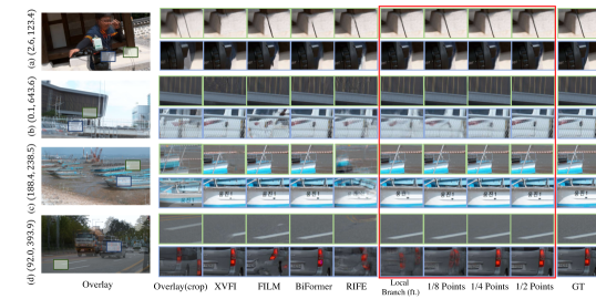
Figure 4: Visual comparison with different methods, instances selected from X-Test-L [29]. We provide the optical flow magnitude on the left, measured by RAFT [32]. Four sparsity setting of our methods lies in the red frame. Blue frames places a greater emphasis on demonstrating large motion, while green frames is more inclined to demonstrate the effect on local details. Best viewed in zoom.

5.4 Ablation Study

In this section, we ablate the effect of our key component, sparse global matching pipeline fintuning, difference map generation in Section 3.2, and merge block in Section 3.5.

Sparse Global Matching. To demonstrate that the primary source of our performance improvements comes from the sparse global matching branch rather than the finetuning process alone, we constructed a Local Branch (ft.) model, incorporating the learnable Flow Refine module (as depicted in Figure 2), to finetune on the X-Train dataset. Our results indicate that while fine-tuning on a large motion dataset can enhance model performance in challenging scenarios with large motion, global matching consistently outperforms it. Furthermore, we present a comprehensive overview of the global matching performance in Table 3. It is evident that as more points are selected, performance reaches saturation, because not every point needs a global receptive field.

Table 3: Comparison of finetuning with different settings. Local Branch (ft.) contains no global matching.

	X-Test-L-2K		X-Test-L-4K
	PSNR	SSIM	PSNR	SSIM
Local Branch (ft.)	30.58	0.8977	29.44	0.8895
1/8 Points	30.83	0.9022	29.73	0.8928
1/4 Points	30.88	0.9043	29.78	0.8948
1/2 Points	30.99	0.9072	29.91	0.8972
Full Global Matching	31.03	0.9074	29.95	0.8974

Difference Map. Our sparse global matching algorithm is guided by difference map, $D_{0}$ and $D_{1}$, which can help us identify flaws in the initial estimation of intermediate flows. We then select the top-$k$ defective points to correct them. To evaluate the effectiveness of the difference map guidance, we conducted a random sampling strategy to replace the map generation and top-$k$ sampling. The results presented in Table 4 demonstrate that selecting random positions for correction is not as effective as choosing the top-$k$ defective points from the difference map. When dealing with sparse points, random sampling can even decrease accuracy by replacing correct flow with an inaccurate flow compensation. As the number of points increases, this gap narrows. Nevertheless, it is still evident that selecting top-$k$ on the difference map outperforms random sampling.

Table 4: Comparison on random sampling $k$ points between generating difference map and sampling top-$k$ points.

	X-Test-L-2K		X-Test-L-4K
	PSNR	SSIM	PSNR	SSIM
Ours-1/2-top-$k$	30.99	0.9072	29.91	0.8972
Ours-1/4-top-$k$	30.88	0.9043	29.78	0.8948
Ours-1/8-top-$k$	30.83	0.9022	29.73	0.8928
Local Branch (ft.)	30.58	0.8977	29.44	0.8895
Ours-1/2-random	30.89	0.9057	29.86	0.8967
Ours-1/4-random	30.67	0.9014	29.55	0.8923
Ours-1/8-random	30.55	0.8992	29.47	0.8893

Flow Merge. To show the effectiveness of our flow merge block, we remove the merge block and directly apply the sparse flow compensation patches $f_{t\rightarrow 0}$ and $f_{t\rightarrow 1}$ on $\widetilde{F}_{t\rightarrow 0}$ and $\widetilde{F}_{t\rightarrow 1}$, respectively. From Table 5, we can see that after removing the merge block, the obtained results still exhibit slightly higher performance than the fine-tuned local branch model, indicating the effectiveness of our flow compensation patches $f_{t\rightarrow 0}$ and $f_{t\rightarrow 1}$. However, it is noteworthy that as we involve more points in the flow compensation, the improvement in results becomes negligible and even falls short of only using 1/8 points, highlighting the necessity of our merge block.

Table 5: Results of our structure with or w/o merge block.

	Merge Block	X-Test-L-2K		X-Test-L-4K
		PSNR	SSIM	PSNR	SSIM
Local Branch (ft.)	$\times$	30.58	0.8977	29.44	0.8895
Local Branch (ft.)	$\surd$	30.55	0.8971	29.44	0.8889
1/8 Points	$\surd$	30.83	0.9022	29.73	0.8995
1/2 Points	$\times$	30.75	0.9025	29.69	0.8936
1/4 Points	$\times$	30.77	0.9014	29.70	0.8924
1/8 Points	$\times$	30.75	0.8992	29.64	0.8910

6 Conclusion

In this paper we have presented a sparse global matching algorithm designed to effectively address the challenges posed by large motion in video frame interpolation. We establish a framework that extracts local features for intermediate flow estimation. Then we target the flaws in the initial flow estimation and perform sparse global matching to produce sparse flow compensation across a global receptive field. By adaptively merging initial intermediate flow estimation with sparse global matching flow compensation, we achieve state-of-the-art performance on the most challenging subset of commonly used large motion datasets while keeping the performance on small-to-medium motion benchmark.

Acknowledgements.

This work is supported by the National Key R$\&$D Program of China (No. 2022ZD0160900), the National Natural Science Foundation of China (No. 62076119, No. 61921006), and Collaborative Innovation Center of Novel Software Technology and Industrialization.

Appendix A Local Feature Branch Model Structure

A.1 Local Feature Extractor

The structure of our local feature extractor is illustrated in Figure A5. As mentioned in Section 3.1, we adopt a CNN and Transformer hybrid structure for local feature extraction. This design diverges from that of EMA-VFI[37] by reducing the network depth. Furthermore, to enhance discriminability within local windows, we incorporate sine-cosine positional embeddings before the windowed cross-attention operation.

A.2 Flow Estimation

The Flow Estimation Structure, depicted in Figure 1, consists of two sequential Flow Estimation blocks, as shown in Figure A6. These two blocks are not identical. The first block, detailed in Figure A6 takes input frames $I_{0},I_{1}\in H\times W\times 3$ and local features $a_{0}^{3},a_{1}^{3}\in H/8\times W/8\times C_{3}$ as input. Its output includes the initial intermediate flow estimations $\widetilde{F}_{t\rightarrow 0},\widetilde{F}_{t\rightarrow 1}$, along with the initial fusion map $\widetilde{M}$.

When pretraining on Vimeo-90K, $\widetilde{F}_{t\rightarrow 0},\widetilde{F}_{t\rightarrow 1}$ and $\widetilde{M}$ are directly fed into the second block, along with warped images $I_{0\rightarrow t},I_{1\rightarrow t}$ and the finer local features $a_{0}^{2},a_{1}^{2}\in H/4\times W/4\times C_{2}$. In the stages of finetuning and inference, however, $\widetilde{F}_{t\rightarrow 0},\widetilde{F}_{t\rightarrow 1}$ and $\widetilde{M}$ are processed by the sparse global matching block for correction, resulting in refined flow estimations $F_{t\rightarrow 0},F_{t\rightarrow 1}$ and an updated fusion map $M$, which are then input to the second block with $I_{0\rightarrow t},I_{1\rightarrow t}$ and $a_{0}^{2},a_{1}^{2}$.

A.3 Refine Net

We follow a similar design in RIFE[9]. We use Context Net to first extract the low-level contextual features. These features are then processed through backward warping, guided by the intermediate flows. The refinement stage involves a U-net shaped network, which can enhance the output frame in a residual form, using the warped features and flows.

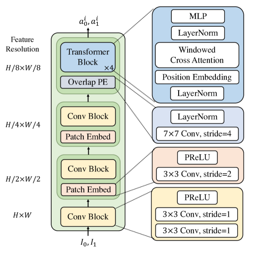
Figure A5: Model Structure of Local Feature Branch. $a^{i}_{0},a^{i}_{1},i\in\{0,1,2,3\}$ is the extracted local feature, corresponding to the feature resolution of $\{H\times W,H/2\times W/2,H/4\times W/4,H/8\times W/8\}$

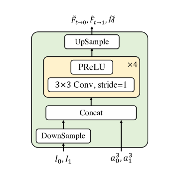
Figure A6: Model Structure of the Initial Flow Estimation Block.

Table A6: Results after applying sparse global matching block on EMA-VFI-small. 1/N means that we sparsely select 1/N points of the initial intermediate flows estimation.

	X-Test-L		SNU-FILM-L		Xiph-L
	2K	4K	hard	extreme	2K	4K
EMA-VFI	29.51/0.8775	28.60/0.8733	28.57/0.9189	23.18/0.8292	30.54/0.8718	28.40/0.8109
EMA-VFI-1/8	29.65/0.8788	28.77/0.8753	28.62/0.9192	23.31/0.8306	30.59/0.8712	28.61/0.8114
EMA-VFI-1/4	29.81/0.8816	28.91/0.8776	28.68/0.9196	23.41/0.8326	30.64/0.8720	28.78/0.8128
EMA-VFI-1/2	30.12/0.8886	29.24/0.8840	28.70/0.9196	23.46/0.8343	30.63/0.8722	28.91/0.8146

Table A7: Results after applying sparse global matching block on RIFE. 1/N means that we sparsely select 1/N points of the initial intermediate flows estimation.

	X-Test-L		SNU-FILM-L		Xiph-L
	2K	4K	hard	extreme	2K	4K
RIFE	29.87/0.8805	28.98/0.8756	28.19/0.9172	22.84/0.8230	30.18/0.8633	28.07/0.7982
RIFE-1/8	30.50/0.8902	29.52/0.8838	28.61/0.9189	23.35/0.8298	30.26/0.8637	28.45/0.8023
RIFE-1/4	30.68/0.8981	29.72/0.8901	28.63/0.9191	23.52/0.8340	30.30/0.8643	28.66/0.8048
RIFE-1/2	30.88/0.9034	29.90/0.8944	28.66/0.9195	23.52/0.8350	30.35/0.8656	28.69/0.8066

Appendix B Model Loss

We use the same training loss with EMA-VFI [37], which is the combination of Laplacian loss and warp loss, defined as:

$$\mathcal{L}=\mathcal{L}_{\text{lap }}+\lambda\sum_{i}\mathcal{L}_{\text{warp }}^{i},$$ (12)

where $\lambda$ is the loss weight for warp loss. Following [37], we set $\lambda$ = 0.5.

Appendix C Generalizability

We apply our sparse global matching block on RIFE[9] and EMA[37] to show that our two-step strategy is applicable in more similar flow-based structures. The result is presented in Table A7 and Table A6 accordingly.

Appendix D Scalability

We scaled our model to a bigger model size with 59.3M parameters, basically aligned with EMA-VFI-base [37] which has 65.7M parameters. Results listed in Table D8. From Table D8, we can draw the following conclusion.

As more points are incorporated into sparse global matching, the performance gradually saturates. This observation is intuitive, considering that not every aspect of the initial estimated flow is inaccurate, nor is every aspect of the global matching flow entirely precise. This is evidenced by Table 5, where the merge block is absent in this ablation. However, upon integrating the merge block (refer to Table 3), with more points are involved, up to full global matching, performance still has a little improvement with increased point involvement, meaning that there is still potential for enhancement within the local branch of the smaller model with the help of our merge block.

But when we change our model with a larger local branch with more parameters, the capacity of the local branch becomes stronger. Consequently, it becomes evident that involving all points in global matching leads to performance degradation compared to utilizing only half the points, thus affirming our pursuit of sparsity.

Table D8: Results on a larger local branch. Note that we disable the test-time augmentation when testing for direct comparison.

	XTest-L-2K
	PSNR	SSIM
EMA-VFI [37]	30.85	0.9005
Ours-local branch	30.68	0.9010
Ours-1/8-Points	31.10	0.9080
Ours-1/4-Points	31.19	0.9102
Ours-1/2-Points	31.27	0.9115
Full Global Matching	31.20	0.9104

Appendix E Model Size Comparisons

We conduct a series of parameters and runtime comparisons on an Nvidia RTX 2080Ti GPU. Illustrated in Table E9, our local branch is aligned with EMA-VFI-small in terms of runtime and parameters, therefore, we mainly compare our results with EMA-VFI-small model setting.

Table E9: Comparisons of model size and corresponding performance. We only list the X-Test-L-2K results for simplicity.

	Inference Time on 512x512 Resolution	Parameters	X-Test-L-2K
			PSNR	SSIM
RIFE	10ms	10M	29.87	0.8805
EMA-VFI-small	25ms	14.5M	29.51	0.8775
EMA-VFI-base	132ms	65.7M	30.85	0.9003
XVFI	22ms	5.6M	29.82	0.8493
BiFormer	59ms	11M	30.32	0.9067
Ours-local-branch	23ms	15.4M	30.39	0.8946
Ours-1/2-Points	74ms	20.8M	30.99	0.9075

Appendix F Different Flow Reversal Teqniques

Table F10: Comparisons between different flow reversal techniques.

	X-Test-L-2K		X-Test-L-4K
	PSNR	SSIM	PSNR	SSIM
flow reversal layer [35]	30.57	0.8977	29.45	0.8886
CFR [29]	30.73	0.9001	29.63	0.8913
linear combination [13]	30.69	0.9000	29.59	0.8907
CNN layer	30.18	0.8932	29.13	0.8853
linear reversal	30.70	0.9017	29.59	0.8924
flow shift (Ours-1/8-Points)	30.83	0.9022	29.73	0.8928

We compare our flow shift strategy with the flow reversal layer in  [35], complementary flow reversal in  [29], linear combination in  [13], CNN layer and linear reversal on Ours-1/8 setting. Shown by Table F10, our flow-shifting strategy is the most suitable for sparsely sampled flows.

Appendix G Interpolating multiple frames into two frames

We follow the recursive interpolation method in FILM [27] and present our multi-frame interpolation (between two frames) results in Table G11.

Table G11: $8\times$ Interpolation Results on X-Test (PSNR).

	X-Test (8$\times$ interpolation)
	2K	4K
EMA-VFI-small-t [37]	31.89	30.89
RIFE-m [9]	31.43	30.58
FILM [27]	31.50	OOM
Ours-1/2-Points	32.38	31.35

Appendix H Finetuning or Training From Scratch

In our experiments, we conducted training from scratch on the Vimeo-90K [4] dataset using a sparse global matching block with full global matching. This approach still demonstrated noticeable effects attributed to the global matching process. However, as indicated in Table H12, the ability to capture large motion was not on par with the results obtained after finetuning on a dataset with larger motion. Therefore, finetuning on a small batch of large motion datasets (X-Train) is more efficient than training from scratch on a large batch of small motion datasets (Vimeo-90K). This efficiency is evidenced by the reduced number of required training steps, with finetuning necessitating only 13.7k steps as opposed to 480k steps for training from scratch. This finding aligns with the observations reported in FILM [27], suggesting that large motion datasets can bring large motion capturing ability.

Table H12: Comparisons between from scratch and finetuning.

	X-Test-L-2K		X-Test-L-4K
	PSNR	SSIM	PSNR	SSIM
Ours-local-branch	30.39	0.8946	29.25	0.8861
Global-From Scratch	30.63	0.9012	29.61	0.8958
Global-Finetuning	31.03	0.9074	29.95	0.8974

Appendix I Failed Matching

When matching fails, the merge block in our method can adaptively merge the flows, depressing the impact of matching failure. Moreover, we have a refine block to further repair the merged flow. We also provide a visualization in Figure I7.

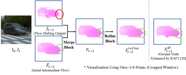
Figure I7: Visualization of Matching Failure and Repair

Appendix J Inference Speed Bottleneck

Operations	Inference Time
Local Feature Branch	23 ms
Flow Compensation Branch	50.6 ms
- Global Feature Extraction	45 ms
- Others	5.6 ms
($512\times 512$ Resolution) Total	73.6ms

Table J13: Time Profile on Our Proposed Algorithm. Measured on an Nvidia RTX 2080Ti GPU.

As shown in Table J13, the bottleneck of our pipeline lies in the global feature extractor, instead of other parameter-free components. One naive solution is to replace it with a simpler and lighter global feature extractor in the future. And another solution is to distill the global feature extraction ability from GMFlow [34] to our own feature extractor, which needs more experiment and probably even training data from optical flow datasets.

References

- Brooks and Barron [2019] Tim Brooks and Jonathan T Barron. Learning to synthesize motion blur. In Proceedings of the IEEE/CVF Conference on Computer Vision and Pattern Recognition, pages 6840–6848, 2019.
- Carion et al. [2020] Nicolas Carion, Francisco Massa, Gabriel Synnaeve, Nicolas Usunier, Alexander Kirillov, and Sergey Zagoruyko. End-to-end object detection with transformers. In European conference on computer vision, pages 213–229, 2020.
- Chen et al. [2022] Zeyuan Chen, Yinbo Chen, Jingwen Liu, Xingqian Xu, Vidit Goel, Zhangyang Wang, Humphrey Shi, and Xiaolong Wang. Videoinr: Learning video implicit neural representation for continuous space-time super-resolution. In Proceedings of the IEEE/CVF Conference on Computer Vision and Pattern Recognition, pages 2047–2057, 2022.
- Choi et al. [2020] Myungsub Choi, Heewon Kim, Bohyung Han, Ning Xu, and Kyoung Mu Lee. Channel attention is all you need for video frame interpolation. In Proceedings of the AAAI Conference on Artificial Intelligence, pages 10663–10671, 2020.
- Chu et al. [2021] Xiangxiang Chu, Zhi Tian, Yuqing Wang, Bo Zhang, Haibing Ren, Xiaolin Wei, Huaxia Xia, and Chunhua Shen. Twins: Revisiting the design of spatial attention in vision transformers. In NeurIPS 2021, 2021.
- Dosovitskiy et al. [2021] Alexey Dosovitskiy, Lucas Beyer, Alexander Kolesnikov, Dirk Weissenborn, Xiaohua Zhai, Thomas Unterthiner, Mostafa Dehghani, Matthias Minderer, Georg Heigold, Sylvain Gelly, Jakob Uszkoreit, and Neil Houlsby. An image is worth 16x16 words: Transformers for image recognition at scale. In International Conference on Learning Representations, 2021.
- Flynn et al. [2016] John Flynn, Ivan Neulander, James Philbin, and Noah Snavely. Deepstereo: Learning to predict new views from the world’s imagery. In Proceedings of the IEEE conference on computer vision and pattern recognition, pages 5515–5524, 2016.
- Hu et al. [2022] Ping Hu, Simon Niklaus, Stan Sclaroff, and Kate Saenko. Many-to-many splatting for efficient video frame interpolation. In Proceedings of the IEEE/CVF Conference on Computer Vision and Pattern Recognition, pages 3553–3562, 2022.
- Huang et al. [2022] Zhewei Huang, Tianyuan Zhang, Wen Heng, Boxin Shi, and Shuchang Zhou. Real-time intermediate flow estimation for video frame interpolation. In European Conference on Computer Vision, pages 624–642, 2022.
- Huang et al. [2024] Zhewei Huang, Ailin Huang, Xiaotao Hu, Chen Hu, Jun Xu, and Shuchang Zhou. Scale-adaptive feature aggregation for efficient space-time video super-resolution. In Winter Conference on Applications of Computer Vision, 2024.
- Hui et al. [2018] Tak-Wai Hui, Xiaoou Tang, and Chen Change Loy. LiteFlowNet: A Lightweight Convolutional Neural Network for Optical Flow Estimation. In Proceedings of IEEE Conference on Computer Vision and Pattern Recognition, pages 8981–8989, 2018.
- Jia et al. [2022] Zhaoyang Jia, Yan Lu, and Houqiang Li. Neighbor correspondence matching for flow-based video frame synthesis. In Proceedings of the 30th ACM International Conference on Multimedia, pages 5389–5397, 2022.
- Jiang et al. [2018] Huaizu Jiang, Deqing Sun, Varun Jampani, Ming-Hsuan Yang, Erik Learned-Miller, and Jan Kautz. Super slomo: High quality estimation of multiple intermediate frames for video interpolation. In Proceedings of the IEEE conference on computer vision and pattern recognition, pages 9000–9008, 2018.
- Jiang et al. [2021] Wei Jiang, Eduard Trulls, Jan Hosang, Andrea Tagliasacchi, and Kwang Moo Yi. Cotr: Correspondence transformer for matching across images. In Proceedings of the IEEE/CVF International Conference on Computer Vision, pages 6207–6217, 2021.
- Jin et al. [2023] Xin Jin, Longhai Wu, Jie Chen, Youxin Chen, Jayoon Koo, and Cheul-hee Hahm. A unified pyramid recurrent network for video frame interpolation. In Proceedings of the IEEE/CVF Conference on Computer Vision and Pattern Recognition, pages 1578–1587, 2023.
- Kim et al. [2022] Hannah Halin Kim, Shuzhi Yu, Shuai Yuan, and Carlo Tomasi. Cross-attention transformer for video interpolation. In Proceedings of the Asian Conference on Computer Vision Workshops, pages 320–337, 2022.
- Kong et al. [2022] Lingtong Kong, Boyuan Jiang, Donghao Luo, Wenqing Chu, Xiaoming Huang, Ying Tai, Chengjie Wang, and Jie Yang. Ifrnet: Intermediate feature refine network for efficient frame interpolation. In Proceedings of the IEEE/CVF Conference on Computer Vision and Pattern Recognition, pages 1969–1978, 2022.
- Li et al. [2023] Zhen Li, Zuo-Liang Zhu, Ling-Hao Han, Qibin Hou, Chun-Le Guo, and Ming-Ming Cheng. Amt: All-pairs multi-field transforms for efficient frame interpolation. In Proceedings of the IEEE/CVF Conference on Computer Vision and Pattern Recognition, pages 9801–9810, 2023.
- Liu et al. [2020] Yihao Liu, Liangbin Xie, Li Siyao, Wenxiu Sun, Yu Qiao, and Chao Dong. Enhanced quadratic video interpolation. In Computer Vision–ECCV 2020 Workshops: Glasgow, UK, August 23–28, 2020, Proceedings, Part IV 16, pages 41–56, 2020.
- Liu et al. [2021] Ze Liu, Yutong Lin, Yue Cao, Han Hu, Yixuan Wei, Zheng Zhang, Stephen Lin, and Baining Guo. Swin transformer: Hierarchical vision transformer using shifted windows. In Proceedings of the IEEE/CVF international conference on computer vision, pages 10012–10022, 2021.
- Lu et al. [2022] Liying Lu, Ruizheng Wu, Huaijia Lin, Jiangbo Lu, and Jiaya Jia. Video frame interpolation with transformer. In Proceedings of the IEEE/CVF Conference on Computer Vision and Pattern Recognition, pages 3532–3542, 2022.
- Montgomery and Lars [1994] Christopher Montgomery and H Lars. Xiph. org video test media (derf’s collection). Online, https://media. xiph. org/video/derf, 6, 1994.
- Niklaus and Liu [2020] Simon Niklaus and Feng Liu. Softmax splatting for video frame interpolation. In Proceedings of the IEEE/CVF Conference on Computer Vision and Pattern Recognition, pages 5437–5446, 2020.
- Park et al. [2020] Junheum Park, Keunsoo Ko, Chul Lee, and Chang-Su Kim. Bmbc: Bilateral motion estimation with bilateral cost volume for video interpolation. In Computer Vision–ECCV 2020: 16th European Conference, Glasgow, UK, August 23–28, 2020, Proceedings, Part XIV 16, pages 109–125, 2020.
- Park et al. [2021] Junheum Park, Chul Lee, and Chang-Su Kim. Asymmetric bilateral motion estimation for video frame interpolation. In Proceedings of the IEEE/CVF International Conference on Computer Vision, pages 14539–14548, 2021.
- Park et al. [2023] Junheum Park, Jintae Kim, and Chang-Su Kim. Biformer: Learning bilateral motion estimation via bilateral transformer for 4k video frame interpolation. In Proceedings of the IEEE/CVF Conference on Computer Vision and Pattern Recognition, pages 1568–1577, 2023.
- Reda et al. [2022] Fitsum Reda, Janne Kontkanen, Eric Tabellion, Deqing Sun, Caroline Pantofaru, and Brian Curless. Film: Frame interpolation for large motion. In European Conference on Computer Vision, pages 250–266, 2022.
- Shi et al. [2022] Zhihao Shi, Xiangyu Xu, Xiaohong Liu, Jun Chen, and Ming-Hsuan Yang. Video frame interpolation transformer. In Proceedings of the IEEE/CVF Conference on Computer Vision and Pattern Recognition, pages 17482–17491, 2022.
- Sim et al. [2021] Hyeonjun Sim, Jihyong Oh, and Munchurl Kim. Xvfi: extreme video frame interpolation. In Proceedings of the IEEE/CVF international conference on computer vision, pages 14489–14498, 2021.
- Siyao et al. [2021] Li Siyao, Shiyu Zhao, Weijiang Yu, Wenxiu Sun, Dimitris Metaxas, Chen Change Loy, and Ziwei Liu. Deep animation video interpolation in the wild. In Proceedings of the IEEE/CVF conference on computer vision and pattern recognition, pages 6587–6595, 2021.
- Sun et al. [2021] Jiaming Sun, Zehong Shen, Yuang Wang, Hujun Bao, and Xiaowei Zhou. Loftr: Detector-free local feature matching with transformers. In Proceedings of the IEEE/CVF conference on computer vision and pattern recognition, pages 8922–8931, 2021.
- Teed and Deng [2020] Zachary Teed and Jia Deng. Raft: Recurrent all-pairs field transforms for optical flow. In Computer Vision–ECCV 2020: 16th European Conference, Glasgow, UK, August 23–28, 2020, Proceedings, Part II 16, pages 402–419, 2020.
- Wu et al. [2018] Chao-Yuan Wu, Nayan Singhal, and Philipp Krahenbuhl. Video compression through image interpolation. In Proceedings of the European conference on computer vision (ECCV), pages 416–431, 2018.
- Xu et al. [2022] Haofei Xu, Jing Zhang, Jianfei Cai, Hamid Rezatofighi, and Dacheng Tao. Gmflow: Learning optical flow via global matching. In Proceedings of the IEEE/CVF conference on computer vision and pattern recognition, pages 8121–8130, 2022.
- Xu et al. [2019] Xiangyu Xu, Li Siyao, Wenxiu Sun, Qian Yin, and Ming-Hsuan Yang. Quadratic video interpolation. Advances in Neural Information Processing Systems, 32, 2019.
- Xue et al. [2019] Tianfan Xue, Baian Chen, Jiajun Wu, Donglai Wei, and William T Freeman. Video enhancement with task-oriented flow. International Journal of Computer Vision, 127:1106–1125, 2019.
- Zhang et al. [2023] Guozhen Zhang, Yuhan Zhu, Haonan Wang, Youxin Chen, Gangshan Wu, and Limin Wang. Extracting motion and appearance via inter-frame attention for efficient video frame interpolation. In Proceedings of the IEEE/CVF Conference on Computer Vision and Pattern Recognition, pages 5682–5692, 2023.
- Zhong et al. [2023] Zhihang Zhong, Mingdeng Cao, Xiang Ji, Yinqiang Zheng, and Imari Sato. Blur interpolation transformer for real-world motion from blur. In Proceedings of the IEEE/CVF Conference on Computer Vision and Pattern Recognition, pages 5713–5723, 2023.
- Zhou et al. [2023] Kun Zhou, Wenbo Li, Xiaoguang Han, and Jiangbo Lu. Exploring motion ambiguity and alignment for high-quality video frame interpolation. In Proceedings of the IEEE/CVF Conference on Computer Vision and Pattern Recognition, pages 22169–22179, 2023.
- Zhu et al. [2021] Xizhou Zhu, Weijie Su, Lewei Lu, Bin Li, Xiaogang Wang, and Jifeng Dai. Deformable detr: Deformable transformers for end-to-end object detection. In International Conference on Learning Representations, 2021.