CaDRec: Contextualized and Debiased Recommender Model
Abstract.
Recommender models aimed at mining users’ behavioral patterns have raised great attention as one of the essential applications in daily life. Recent work on graph neural networks (GNNs) or debiasing methods has attained remarkable gains. However, they still suffer from (1) over-smoothing node embeddings caused by recursive convolutions with GNNs, and (2) the skewed distribution of interactions due to popularity and user-individual biases. This paper proposes a contextualized and debiased recommender model (CaDRec). To overcome the over-smoothing issue, we explore a novel hypergraph convolution operator that can select effective neighbors during convolution by introducing both structural context and sequential context. To tackle the skewed distribution, we propose two strategies for disentangling interactions: (1) modeling individual biases to learn unbiased item embeddings, and (2) incorporating item popularity with positional encoding. Moreover, we mathematically show that the imbalance of the gradients to update item embeddings exacerbates the popularity bias, thus adopting regularization and weighting schemes as solutions. Extensive experiments on four datasets demonstrate the superiority of the CaDRec against state-of-the-art (SOTA) methods. Our source code and data are released at https://github.com/WangXFng/CaDRec.
1. Introduction
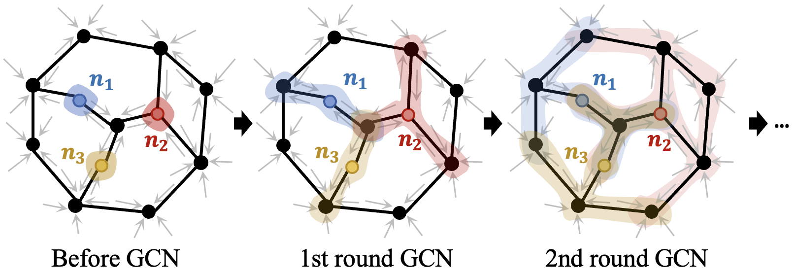
With information overload via Internet services, recommender systems have become inevitable applications in daily life. A reliable recommender system should provide high-quality results by mining behavioral patterns from limited users’ interactive histories. One typical approach is to leverage graph convolution networks (GCNs) to propagate node embeddings through user–item interaction edges to capture collaborative signals (He et al., 2020; Hao et al., 2021; Yu et al., 2022b), e.g., self-supervised graph learning (Yu et al., 2021a), and hypergraph convolutions (Xia et al., 2022b, a; Yan et al., 2023). However, they still suffer from over-smoothing issues caused by iterative convolutions over a sparse user–item interactive graph based on a static adjacency matrix. As depicted in Fig. 1, given a subgraph with the maximum shortest path of 4, after two rounds of GCN operations, the features of nodes , , and have propagated across the entire subgraph, resulting in plenty of nodes having similar information and being overly uniform (smooth), as highlighted by blue, red, and yellow edges. To address the issue, several attempts including users’ common interests mining (Liu et al., 2021b), graph structure augmentations (Wu et al., 2021), and node augmentations (Yu et al., 2022a, 2023; Lin et al., 2022; Cai et al., 2023), have been made to increase the dispersion of node embeddings to capture discernible collaborative signals through GCNs.
However, one major drawback of GCN operators in the approaches mentioned above is that they cannot capture the sequential dependencies of neighbors but only the connectivity between two nodes, even though sequential contexts are an important clue to mitigate over-smoothing issues. For instance, once a user completes the initial volume of a book or movie, it’s quite natural that the system would likely suggest its sequel. As shown in Fig. 1, if node refers to a random neighbor and serves as a sequel of , a user who has finished experiencing is more likely to prefer than . This suggests that has a more contextual relationship with in sequential dependencies, compared to in the GCN graph. The attention mechanism is one solution to capture the sequential dependencies. Several algorithms including graph attention network (GAN)-based techniques (Wu et al., 2019; Chen et al., 2022a) have been proposed to select representative items from users’ massive sequential interactions that can reflect their preferences (Tao et al., 2022; Wang et al., 2023b). More recently, (Xia et al., 2022b; Wang et al., 2023a) incorporated transformers with GCNs. All of the approaches gained inspiring results. However, they select ineffective items in the way of modeling user–item interaction as they ignore that both structural and sequential contexts help derive more effective node embeddings during graph convolution.
Another issue is skewed interaction distribution, in which the user–item interaction susceptibly falls into due to diversified biases (Chen et al., 2021), e.g., popularity bias, resulting in deviating user representations from their true preferences. One attempt is to disentangle the real properties of items from the popularity impacts (Ren et al., 2022; He et al., 2022; Cao et al., 2022; Zhang et al., 2023b). It employs two independent neural encoders to tokenize the properties and popularity of items. However, they ensure only the separation of popularity and item representations. Such neural encoders might have learned other factors (e.g., gender and age in fairness-aware recommendations (Li et al., 2021; Wang et al., 2023c)) instead of item popularity. Moreover, most of the disentangling approaches do not pay attention to user individual biases. For instance, given the objective scores of (4, 5, 3, 3) which indicate real properties of four items, if an optimistic user gives over-high rating scores, (5, 5, 4, 5), and a serious user leaves critical reviews and rate them with the scores of (3, 5, 1, 2), the individual biases of these two users are (+1, 0, +1, +2) and (-1, 0, -2, -1), respectively, resulting in harmful to understanding the semantic properties of items correctly. Therefore, disentangling the popularity and user individual biases is essential for mining users’ true preferences and item real properties.
In this paper, we propose a contextualized and debiased representation learning network (CaDRec). Instead of simply employing stacked Transformers behind hypergraph convolutions (HGCs) (Xia et al., 2022a; Wang et al., 2023a), our approach involves injecting the self-attention (SA) correlation, which serves as a trainable perturbation (Goodfellow et al., 2014; Yu et al., 2023) on edges representing sequential relations among nodes, into convolution operators. This is motivated by our decomposition of the operations of HGC and SA, revealing that both operations facilitate informative diffusion relying on two correlation matrices of the same size, although they are distributed in entirely different spaces. Thus, the HGC operators consider both structural and sequential contexts among neighboring nodes to propagate messages, rather than relying solely on a static adjacency matrix, aiming to break through the over-smoothing bottleneck in HGC.
To make debiased recommendations, we propose two novel strategies to disentangle user–item interactions: (1) in addition to popularity bias (Chen et al., 2022b; He et al., 2022; Zhao et al., 2022), we model user individual bias to promote debiased item representations, and (2) the popularity of an item is encoded through its interaction count with positional encoding (Vaswani et al., 2017), which is plug-and-play and interpretable, ensuring that the items of similar popularity are closer in the embedding space. The CaDRec fits the popularity and user individual biases during training, while it generates a recommended list via debiased representations of users and items in testing. The main contributions of our work can be summarized as follows:
(1) To mitigate over-smooth graph embeddings, we propose a novel HGC operator that effectively propagates information during GCN by considering both structural and sequential contexts.
(2) To overcome the distribution shift caused by popularity and user-individual biases, we propose an interpretable disentanglement method to derive debiased representations.
(3) We verify that the imbalance of the gradients to update item embeddings exacerbates the popularity bias whereby adopting regularization and weighting schemes as solutions.
(4) Extensive experiments on four real-world public datasets demonstrate that the CaDRec outperforms SOTA methods with the efficiency of time complexity.
2. Related Work
Recommendation Approaches for Over-Smoothing Issue. The GCN-based methods are prone to the over-smoothing issue, i.e. node embeddings are similar and difficult to discriminate from each other (Keriven, 2022). To mitigate the issue, Liu et al. (2021b) have attempted to utilize the common interests between high-order adjacent users to enhance embedding learning in GCN. Several attempts (Yu et al., 2021a, b; Wu et al., 2021; Peng et al., 2022; Wang et al., 2022) have explored self-supervised learning techniques to boost the robustness of node embeddings. Contrastive augmentations also attracted intensive attention for enhancing the dispersion of node embeddings via contrastive views, such as nodes with their structural neighbors (Lin et al., 2022), node embeddings with and without uniform noise (Yu et al., 2022a, 2023), and SVD-guided contrastive pairs (Cai et al., 2023). Likewise, Wang et al. (2023a) mine implicit features to make node embeddings more distinctive. However, most of the approaches overlook that sequential contexts give a dynamic sequential diversity which boosts graph-based contexts to select effective neighbors during graph convolutions.
Recommendation Approaches for Debiasing. Recommender models are vulnerable to several biases (Chen et al., 2021), such as popularity and exposure biases, which result in severe performance drops. To generalize popularity, many works independentize representations of popularity and item property via orthogonal constraints, such as cosine similarity (Ren et al., 2022; Zhang et al., 2023b), inner product (Chen et al., 2022b), curriculum learning (Zheng et al., 2021), information theory (Cao et al., 2022), and anti-preference negative sampling (He et al., 2022). They utilize two neural encoders for the separation of popularity and item representations. However, these encoders might have learned factors (e.g., gender and age) other than popularity. Besides, several theoretical tools have been explored for debiasing recommendations, such as information bottlenecks (Liu et al., 2021a, 2023), inverse propensity scores (Ding et al., 2022; Zhang et al., 2023a), upper bound minimization (Xiao et al., 2022), bias-aware contrastive learning (Zhang et al., 2022), causal analysis (Li et al., 2023), and quantitative metric (Zhou et al., 2023). Qiu et al. (2022) and Zhang et al. (2024) optimize representation distributions for debaising by counteracting dimensional collapse and embedding degeneration. Most of the above algorithms overlook that the item representations learned from the data distribution are impeded by user-individual bias. Our decomposition technique is motivated by Zheng et al. (2021). The difference is that we incorporate the individual bias and encode popularity with positional encoding.
3. Preliminaries
3.1. Definitions
(User Individual Bias). represents the individual bias of user (), denotes an embedding matrix, and refers to the dimension size.
(Item Popularity). The popularity embedding of item is encoded with its global activeness (i.e., its count of interactions, ) by using the positional encoding, where the element at index is for odd and for even .
(Item Recommendation). Given a user set , an item set , and a user historical interaction set , where denotes the item sequence of user , and refers to the number of items, the goal is to generate a list of the top- candidate items for user .
3.2. Perturbation for Modeling Individual Bias
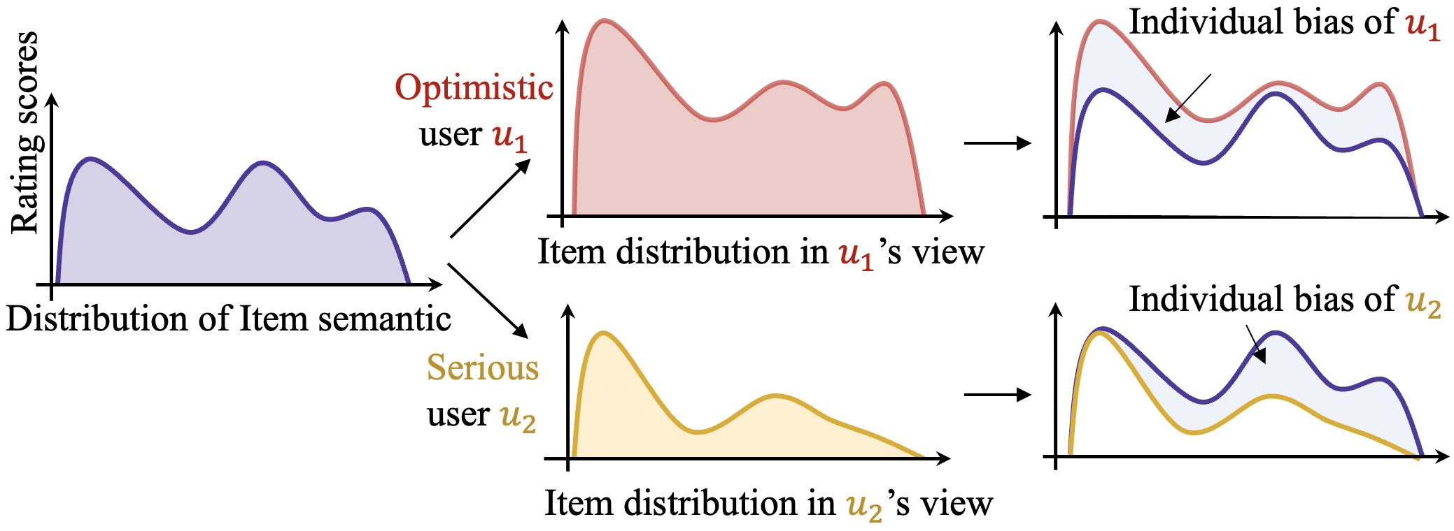
It is often the case that observational interaction distributions are skewed due to diversified latent factors, such as popularity and exposure bias (Chen et al., 2021). These latent factors are well-studied in recent years (Ren et al., 2022; Zhang et al., 2023b; Xiao et al., 2022; Zhang et al., 2023a). However, they do not mention that optimistic users often give high rating scores while serious people may not, even for the same items, which will prevent capturing semantic properties of preference correctly. In Fig. 2, the distribution of item real semantics about its objective rating score is distinct (depicted in purple). However, real-world situations often introduce a user-individual bias (depicted in grey) in this distribution between the item real semantics distribution (in purple color) and the observed item distributions (in red and yellow colors) from users’ interactive behaviors. This bias is harmful to understanding items’ real semantics for recommender algorithms.
These observations indicate that the observed item distribution in each user’s perspective is determined by the item semantic distribution and the user-individual bias. We thus assume that individual bias is a learnable perturbation on item representations when simulating the user-item interactions via graph convolutions. Perturbation learning is widely utilized to bolster the robustness and generalization capabilities of models, such as word-level enhancement (Huang et al., 2022), image noise injection (Song et al., 2023), and node embedding augmentation in recommendation tasks (Yu et al., 2022a, 2023). Therefore, by urging the learnable perturbation to converge to user-individual bias, we can obtain a robust item semantic distribution that is free from being entangled in individual biases.
It is noteworthy that user-individual bias as an important clue of user preferences is leveraged to generate user representations in both training and test stages.
4. Methodology
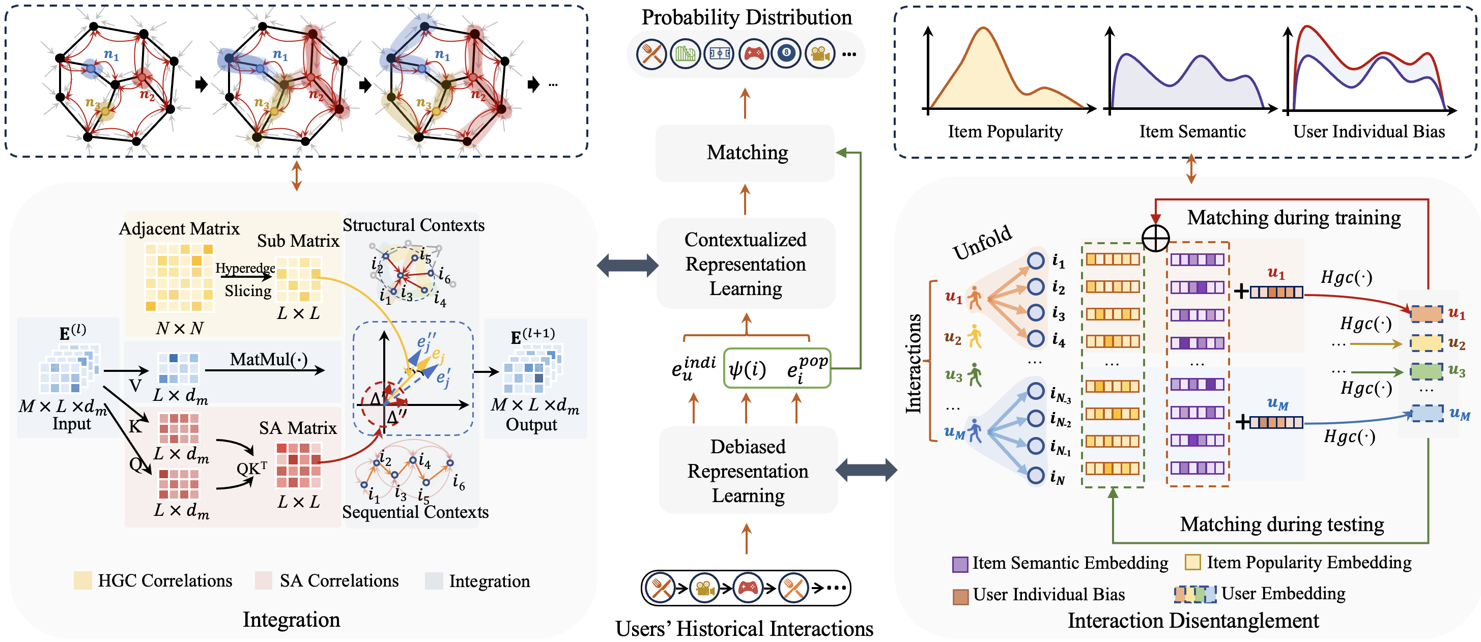
Fig. 3 illustrates the framework of CaDRec, consisting of contextualized representation learning and debiased representation learning.
4.1. Model Basics
The CaDRec adopts a dot-product model as its backbone, which estimates the preference of a user for an item by an inner-product between the embeddings of user and item :
| (1) |
where and are the embeddings of and , respectively. and denote the feature mappings of the model. We initiate item embeddings by the uniform distribution and exert users’ historical interactions to generate user embeddings via , which are given by:
| (2) |
4.2. Contextualized Representation Learning
We first introduce the hypergraph convolution (HGC), the relation between HGC and Transformer, and their incorporation. We then show the process of learning users’ contextualized representations.
Graph Convolution (GCN). Following the works by (He et al., 2020; Wang et al., 2023a), we removed the global weight matrix and added a linear feature transformation (). The matrix equivalence form of informative diffusion in the GCN is as follows:
| (3) |
where indicates the output of the -th GCN layer, is the ELU activation function, and denotes the symmetrically normalized adjacency matrix:
| (4) |
where denotes the adjacency matrix, in which , if the same user has interacted with item and item , otherwise 0. refers to the diagonal matrix in which each entry indicates the number of nonzero entries in the -th row of .
Hypergraph Convolution (HGC). Inspired by the EEDN (Wang et al., 2023a), we utilized a user hypergraph to enhance signal propagation during GCN via learning local contexts from user hyperedges. Note that the multiplication of and a hyperedge can be implemented by the slicing operation that selects corresponding rows in . Thus, and are substituted by , and , respectively:
| (5) | ||||
where refers to the slicing operation and indicates the hyperedge of the user . As the slicing operation takes , the computational complexity of HGC reduces from to , where . Nevertheless, the HGC cannot handle the over-smoothing issue caused by iterative message-passing over the static structural graph.
Integration of HGC and SA. Indeed, there exists a strong underlying relation between HGC and Transformer, in the sense that these two paradigms aggregated the input signals with weight by two correlation matrices of the same size. Specifically, the sub adjacency matrix refers to the structural relationships between items within the user’s hyperedge, while the SA matrix learns the sequential dependencies between the user’s historical interactions. However, these relations are distributed from completely different spaces. Inspired by the random perturbation (Goodfellow et al., 2014; Yu et al., 2023), we exert the SA relation as a perturbation to aid the GCN operator in selecting effective neighbors, as the integration module depicted in Fig. 3. Thus, informative diffusion is given by:
| (6) | ||||
where and are weight matrices, indicates L2 normalization, and is a hyperparameter. As such, HGC can promote diverse representations by considering both structural and sequential contexts, with a time complexity reduced from to +. The multi-head (MH) block is used to learn features in multiple subspaces. The is given by the following equation:
| (7) |
where denotes the number of heads. A simple summation as the aggregation function works better than a feed-forward network.
Consider the item embeddings as the input of the first HGC layer, and we obtain user ’s embedding by feeding the output of the last HGC layer into an average-pooling layer and L2 normalization layer as follows:
| (8) |
To exploit sequential contexts, we adopt a multi-label cross-entropy loss instead of the widely used Bayesian personalized ranking (BPR) loss (Rendle et al., 2012) as the objective function:
| (9) |
where refers to a true label vector, and each dimension of the vector equals 1 when the user has ever visited the item; otherwise, 0. is the activation function.
4.3. Debiased Representation Learning
We introduce two debiasing methods, i.e., interaction disentanglement and embedding debiasing to enhance recommendations.
Interaction Disentanglement. As shown in Fig. 3, we built three tokens to disentangle interactions: user individual bias, item popularity, and item real semantic. To disentangle item representations from user individual bias, similar to Eq. (6), we regard as a learnable perturbation to the items’ real semantics to fitting biased interactions. The feature vector of user is given by:
| (10) | ||||
where denotes the representation of the HGC with injecting SA. learns the individual bias of user such that has less individual bias, and is a broadcast multiplication.
We assume that the user embedding has little popularity. Therefore, we do not take into account and for testing. We refined the rating score as follows:
| (11) |
where denotes a concatenation and is a hyperparameter that varies the influence level of popularity. Here, denotes the pure preference of user , and the real semantic of item is free from being entangled in popularity and user-individual biases.
Debiasing on Embeddings. We revisit the gradient of the rating loss for the embeddings (i.e., user or item embeddings) as follows:
| (12) | ||||
We further define the user embeddings as , and the embeddings of items that users have InterActed (IA) and Future-InterActed (FIA) as and , respectively. Note that (1) a user’s embedding is learned from the user’s IA items through , (2) negative samples have been filtered out by , and (3) is a constant matrix for . We thus derive , , and . To sum up, the gradients for updating embeddings are as follows:
| (13) | ||||
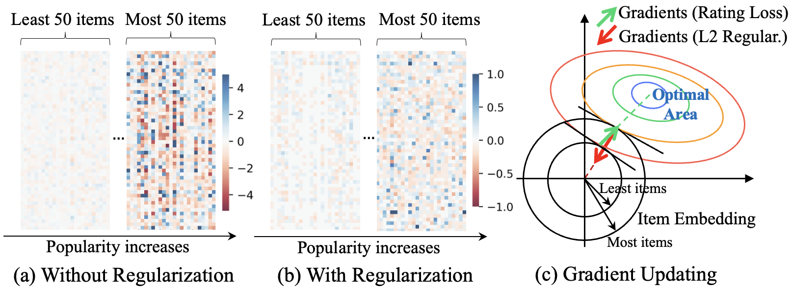
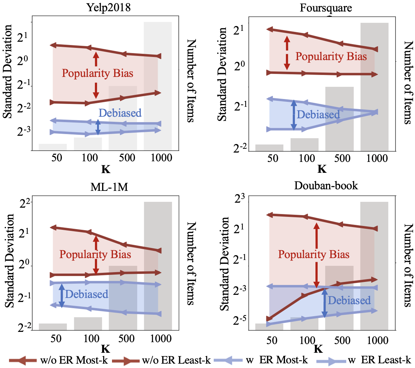
Through the derivation, we observed two issues in the vanilla multi-label cross-entropy function. The first issue is that there are no penalties for negative samples, resulting from a of 0 for a negative sample , while a positive sample could be a negative sample for another user. This makes the popular items overly encouraged. In Fig. 4 (a), we can see that the variance of embedding vectors obtained by the 50 most popular items was significantly larger than that of the 50 least popular items. This indicates that the value of the inner products of the feature vectors of any user and popular items is likely to be a larger value than those of unpopular ones, resulting in the model recommending the most popular items over users’ pure preferences. More specifically, the blue circle in Fig. 4 (c) indicates the optimal area for item embeddings on the training set, while they are overfitting caused by the popularity bias. To address this issue, we employed L2 regularization to the positive samples (i.e., the IA items) during the training stage. Formally, given the indicator function , the learning rate , the hyperparameter of to control the penalization level, and the user set in the training batch, the gradients to update are formulated as follows:
| (14) |
As such, the rating loss term enables item embeddings to learn real semantic, i.e., embeddings are updated in the correct direction, as illustrated in the green arrow of Fig. 4 (c). Simultaneously, the regularization term prevents popular items from being overweighted by reducing the embedding complexity, which is shown in the red arrow. As illustrated in (a) and (b), we empirically showed significant mitigation of gradient imbalance between the most and least popular item embeddings after regularization.
The second issue is that the gradients for updating IA and FIA item embeddings are often imbalanced as there is always one more term, i.e., , for the IA items. Thus, we utilize a weighting scheme (Ma et al., 2018; Wang et al., 2023a) to balance the gradients. The final loss function is given by:
| (15) |
where denotes the element-wise multiplication and refers to L2 regularization. is given by:
| (16) |
where and are two hyperparameters used to balance the weights between the IA and FIA items for users.
5. Experiment
| Dataset | #User | #Item | #Interaction | #Avg. | Density |
|---|---|---|---|---|---|
| Yelp2018 | 31,668 | 38,048 | 1,561,406 | 49.3 | 0.13% |
| Foursquare | 7,642 | 28,483 | 512,532 | 68.2 | 0.24% |
| Douban-book | 12,859 | 22,294 | 598,420 | 46.5 | 0.21% |
| ML-1M | 6,038 | 3,533 | 575,281 | 95.3 | 2.7% |
| Metric | GCN-based | SA-based | Diff-based | Debias-based | Over-smoothing alleviation (OSA)-based | CaDRec | ||||||||||
|---|---|---|---|---|---|---|---|---|---|---|---|---|---|---|---|---|
| LightGCN | LCFN | AutoCF | STaTRL | DiffRec | DICE | InvCF | LightGCL | SGL | IMPGCN | GDE | HCCF | NCL | XSimGCL | EEDN | (ours) | |
| Yelp2018 | ||||||||||||||||
| R@5 | 0.0191 | 0.0209 | 0.0221 | 0.0215 | 0.0236 | 0.0204 | 0.0213 | 0.0195 | 0.0220 | 0.0188 | 0.0175 | 0.0221 | 0.0223 | 0.0251 | 0.0267 | 0.0275 |
| N@5 | 0.0371 | 0.0385 | 0.0420 | 0.0415 | 0.0402 | 0.0356 | 0.0399 | 0.0393 | 0.0421 | 0.0354 | 0.0329 | 0.0425 | 0.0428 | 0.0478 | 0.0508 | 0.0533 |
| R@10 | 0.0347 | 0.0357 | 0.0391 | 0.0372 | 0.0414 | 0.0320 | 0.0377 | 0.0372 | 0.0384 | 0.0293 | 0.0280 | 0.0394 | 0.0390 | 0.0445 | 0.0457 | 0.0474 |
| N@10 | 0.0397 | 0.0378 | 0.0447 | 0.0420 | 0.0471 | 0.0401 | 0.0433 | 0.0414 | 0.0447 | 0.0343 | 0.0339 | 0.0454 | 0.0456 | 0.0502 | 0.0531 | 0.0558 |
| R@20 | 0.0582 | 0.0564 | 0.0662 | 0.0662 | 0.0693 | 0.0570 | 0.0657 | 0.0674 | 0.0659 | 0.0504 | 0.0490 | 0.0688 | 0.0665 | 0.0745 | 0.0760 | 0.0792 |
| N@20 | 0.0484 | 0.0476 | 0.0546 | 0.0501 | 0.0586 | 0.0410 | 0.0543 | 0.0587 | 0.0549 | 0.0400 | 0.0375 | 0.0565 | 0.0558 | 0.0635 | 0.0639 | 0.0667 |
| Foursquare | ||||||||||||||||
| R@5 | 0.0480 | 0.0506 | 0.0473 | 0.0472 | 0.0492 | 0.0498 | 0.0419 | 0.0487 | 0.0471 | 0.0371 | 0.0351 | 0.0489 | 0.0511 | 0.0459 | 0.0554 | 0.0561 |
| N@5 | 0.0784 | 0.0786 | 0.0743 | 0.0763 | 0.0773 | 0.0702 | 0.0625 | 0.0765 | 0.0753 | 0.0607 | 0.0571 | 0.0785 | 0.0834 | 0.0721 | 0.0867 | 0.0879 |
| R@10 | 0.0725 | 0.0731 | 0.0741 | 0.0735 | 0.0744 | 0.0750 | 0.0677 | 0.0719 | 0.0728 | 0.0660 | 0.0626 | 0.0777 | 0.0788 | 0.0727 | 0.0852 | 0.0867 |
| N@10 | 0.0795 | 0.0769 | 0.0771 | 0.0778 | 0.0790 | 0.0732 | 0.0681 | 0.0777 | 0.0772 | 0.0743 | 0.0710 | 0.0759 | 0.0854 | 0.0755 | 0.0886 | 0.0898 |
| R@20 | 0.1094 | 0.1165 | 0.1121 | 0.1106 | 0.1102 | 0.1010 | 0.1069 | 0.1067 | 0.1102 | 0.0968 | 0.0943 | 0.1121 | 0.1206 | 0.1138 | 0.1270 | 0.1314 |
| N@20 | 0.0934 | 0.0924 | 0.0904 | 0.0916 | 0.0921 | 0.0827 | 0.0828 | 0.0920 | 0.0914 | 0.0868 | 0.0796 | 0.0964 | 0.1012 | 0.0905 | 0.1047 | 0.1068 |
| Douban-book | ||||||||||||||||
| R@5 | 0.0640 | 0.0623 | 0.0615 | 0.0693 | 0.0650 | 0.0667 | 0.0654 | 0.0666 | 0.0790 | 0.0551 | 0.0455 | 0.0756 | 0.0930 | 0.1019 | 0.1015 | 0.1055 |
| N@5 | 0.1170 | 0.1150 | 0.1215 | 0.1370 | 0.1225 | 0.1288 | 0.1192 | 0.1290 | 0.1426 | 0.1038 | 0.0996 | 0.1406 | 0.1661 | 0.1901 | 0.1912 | 0.2018 |
| R@10 | 0.0972 | 0.0992 | 0.0927 | 0.0994 | 0.0956 | 0.1036 | 0.1089 | 0.1145 | 0.1189 | 0.0884 | 0.0740 | 0.1168 | 0.1340 | 0.1448 | 0.1450 | 0.1504 |
| N@10 | 0.1165 | 0.1123 | 0.1175 | 0.1286 | 0.1180 | 0.1221 | 0.1199 | 0.1452 | 0.1418 | 0.1056 | 0.1005 | 0.1416 | 0.1625 | 0.1817 | 0.1822 | 0.1918 |
| R@20 | 0.1455 | 0.1457 | 0.1344 | 0.1401 | 0.1369 | 0.1520 | 0.1410 | 0.1624 | 0.1713 | 0.1293 | 0.1146 | 0.1747 | 0.1898 | 0.1989 | 0.1954 | 0.2085 |
| N@20 | 0.1253 | 0.1368 | 0.1240 | 0.1313 | 0.1228 | 0.1409 | 0.1356 | 0.1501 | 0.1514 | 0.1105 | 0.1497 | 0.1585 | 0.1713 | 0.1867 | 0.1852 | 0.1960 |
| ML-1M | ||||||||||||||||
| R@5 | 0.1067 | 0.0879 | 0.0927 | 0.0913 | 0.0984 | 0.0998 | 0.0935 | 0.1025 | 0.1111 | 0.1007 | 0.0981 | 0.0959 | 0.1128 | 0.1161 | 0.1075 | 0.1220 |
| N@5 | 0.3237 | 0.2653 | 0.2728 | 0.2614 | 0.2893 | 0.2876 | 0.2827 | 0.3210 | 0.3304 | 0.2488 | 0.2891 | 0.2819 | 0.3419 | 0.3379 | 0.3052 | 0.3506 |
| R@10 | 0.1708 | 0.1450 | 0.1599 | 0.1535 | 0.1530 | 0.1677 | 0.1617 | 0.1687 | 0.1751 | 0.1493 | 0.1608 | 0.1607 | 0.1800 | 0.1834 | 0.1675 | 0.1933 |
| N@10 | 0.3057 | 0.2450 | 0.2621 | 0.2518 | 0.2673 | 0.2690 | 0.2663 | 0.2997 | 0.3110 | 0.2478 | 0.2977 | 0.2585 | 0.3224 | 0.3210 | 0.2723 | 0.3281 |
| R@20 | 0.2622 | 0.2358 | 0.2287 | 0.2423 | 0.2276 | 0.2514 | 0.2361 | 0.2517 | 0.2622 | 0.2317 | 0.2509 | 0.2321 | 0.2727 | 0.2747 | 0.2665 | 0.2907 |
| N@20 | 0.3076 | 0.2556 | 0.2686 | 0.2603 | 0.2622 | 0.2863 | 0.2703 | 0.3002 | 0.3120 | 0.2628 | 0.2799 | 0.2706 | 0.3227 | 0.3203 | 0.2927 | 0.3261 |
5.1. Experimental Setup
Datasets. We performed the experiments on four benchmark datasets: Yelp2018 (He et al., 2020; Yu et al., 2023; Wang et al., 2023a), Foursquare (Wang et al., 2023a), Douban-book (Yu et al., 2021a, 2023), and ML-1M (Lin et al., 2022). The data statistics are shown in Table 1. Following related work (Wang et al., 2023a, b; Yu et al., 2023), we used the earliest 70% check-ins as training data, the most recent 20% check-ins as test data, and the remaining 10% as validation data for each user. For baselines that obtain the best performance in the training and test sets with a ratio of 8:2, we merged our training and validation set as a training set. Their test set is the same as our model. We used two metrics: Recall@ (R@) and NDCG@ (N@) with {5,10,20}.
Baselines. We compared our CaDRec with the following fifteen related works as baselines which are divided into five groups:
- •
- •
-
•
Diffusion (Diff)-based methods: DiffRec (Wang et al., 2023d) learns the generative process in a denoising manner for recommendations.
-
•
Debiasing (Debias)-based methods: (1) DICE (Zheng et al., 2021) structurally disentangles interest and conformity to recommend items, (2) InvCF (Zhang et al., 2023b) disentangles representations of preference and popularity semantics, and (3) LightGCL (Cai et al., 2023) impairs the model’s generality and robustness via a light contrastive paradigm;
-
•
Over-smoothing alleviation (OSA)-based methods: (1) SGL (Wu et al., 2021) reinforces node representations via self-discrimination, (2) IMP-GCN (Liu et al., 2021b) performs GCNs inside subgraphs with users’ similar interests, (3) GDE (Peng et al., 2022) replaces neighborhood aggregation with a denoising filter, (4) HCCF (Xia et al., 2022b) exploits cross-view contrastive hypergraphs to learn collaborative relations, (5) NCL (Lin et al., 2022) regards users (or items) and their structural neighbors as contrastive pairs, (6) XSimGCL (Yu et al., 2023) creates contrastive views to add uniform noise into embedding spaces, and (7) EEDN (Wang et al., 2023a) mines implicit features to learn rich interactive features between users and items.
Implementation. The best hyperparameters of the CaDRec were sampled as follows: is 0.1 for Foursquare and Douban-book, 0.5 for Yelp2018, and 0 for ML-1M. , , , and were set to 0.25, 0.6, 2.3, and 7.0 for Yelp2018, 0.7, 0.05, 0.33, and 0.44 for Foursquare, 0.4, 0.06, 0.46 and 0.41 for ML-1M, and 0.07, 0.65, 0.98, and 0.75 for Douban-book, respectively. was 768 for Foursquare and 512 for the others. The learning rate was 1e-2. The number of HGC layers was 1, and the number of heads was set to 3 and 2 for Foursquare and ML-1M, and 1 for others. These hyperparameters were tuned using Optuna111https://github.com/pfnet/optuna. The parameters for the baselines were tuned to attain the best performance or set as reported in the original papers. For a fair evaluation, we conducted each experiment five times and obtained the average result. We implemented the CaDRec with Pytorch and experimented on the Nvidia GeForce RTX 3090 (24GB memory).
5.2. Experimental Results
We compared our method with SOTA recommender approaches. The results are displayed in Table 2. We can see that CaDRec is consistently superior to all baselines, specifically, the improvements compared with the runner-ups EEDN, NCL, and XSimGCL were 3.7% 5.3% on Yelp2018, 1.3% 3.5% on Foursquare, 3.6% 5.5% on Douban-book, and 1.1% 8.2% on ML-1M in terms of R@ and N@, where = 5, 10, and 20. The results support our hypothesis that CaDRec is effective for (1) mitigating over-smoothing by incorporating sequential information into GCN operators, and (2) eliminating the impact of popularity while disentangling item representations from user individual biases. Table 2 also promotes the following observations and insights:
-
•
The OSA-based baselines attempt to address the over-smoothing issue by performing graph augmentations on nodes, edges, or structures. However, they are less effective than CaDRec for two possible reasons: (1) their GCN operators solely propagate messages on the connectivity between nodes, and (2) the representations learned by their graph learning are impeded by popularity and individual bias.
-
•
Both InvCF and DICE utilize two neural encoders to independentize the representations of preference and popularity for debiasing. In contrast, the CaDRec tokenizes historical item activeness as popularity representations via positional encoding. The LightGCL employs singular value decomposition (SVD) to align graph contrastive learning representations for popularity debiasing, disregarding the effective sequential context for GCNs.
-
•
Note that EEDN and HCCF explore beyond pair-wise relations between users and items via hypergraphs. However, EEDN, which additionally leverages sequential contexts, achieves remarkable performance, highlighting the effectiveness of sequential contexts in enriching user representations. In contrast, the results of SA-based models indicate that relying solely on sequential patterns is insufficient to provide accurate recommendations.
-
•
The GCL-based methods, NCL and XSimGCL, are competitive among baselines. This implies that the contrast of pairs, e.g. a node and its neighbors, contributes to the generalizability of graph embeddings making nodes more distinctive.
-
•
The SGL, NCL, LightGCL, and XSimGCL introduce the InfoNCE loss, while they perform worse than the CaDRec, indicating advantages of the CaDRec loss: (1) it discriminatively encourages positive samples instead of penalizing stochastic candidates, which could be the false-negative items that users prefer, (2) it properly regularizes positive samples to avoid overfitting the popularity bias, and (3) it enables the injection of sequential contexts to enrich user representations.
-
•
Although DiffRec effectively denoises user–item interactions via generative learning, it is fairly limited by insufficient prior knowledge, various contexts, and debiases.
| Model | Yelp2018 | Foursquare | ML-1M | Douban-book | ||||
|---|---|---|---|---|---|---|---|---|
| R@20 | N@20 | R@20 | N@20 | R@20 | N@20 | R@20 | N@20 | |
| w/o SA | 0.0775 | 0.0649 | 0.1282 | 0.1039 | 0.2907 | 0.3261 | 0.1954 | 0.1846 |
| w/o Dis | 0.0759 | 0.0632 | 0.1238 | 0.1010 | 0.2593 | 0.2913 | 0.1933 | 0.1816 |
| w/o ER | 0.0720 | 0.0605 | 0.1217 | 0.1002 | 0.2580 | 0.2921 | 0.1713 | 0.1632 |
| w/o WS | 0.0751 | 0.0622 | 0.1273 | 0.1044 | 0.2795 | 0.3152 | 0.2038 | 0.1919 |
| Full | 0.0792 | 0.0668 | 0.1314 | 0.1068 | 0.2907 | 0.3261 | 0.2085 | 0.1960 |
5.3. Ablation Study
Table 3 shows an ablation study to examine the effect of each module on the CaDRec, which provides the following observations:
-
•
We can see that in most cases, i.e., on the Yelp2018, Foursquare, and Douban-book datasets, the SA correlation as auxiliary information greatly enhances the ability to select effective neighbors and further alleviates the over-smoothing issue.
-
•
The comparative results of CaDRec with and without interaction disentanglement indicate that the disentanglement contributes to promoting performance. It poses the essentiality of decoupling items’ embeddings from popularity influences and user individual bias for recommendations.
-
•
The CaDRec without embedding regularization is affected by popularity bias, and its performance drops significantly, suggesting that regularization is effective for correcting gradient propagations to update embeddings.
-
•
The results without a weighting scheme, i.e., “w/o WS”, are in underperformance, indicating that balancing the gradients of updating IA and FIA item embeddings noticeably reinforces debiased representations for recommendations.
5.4. Further Analysis of CaDRec
| Category | Yelp2018 | Foursquare | ML-1M | Douban-book | |||||
|---|---|---|---|---|---|---|---|---|---|
| Pop | Indi | R@20 | N@20 | R@20 | N@20 | R@20 | N@20 | R@20 | N@20 |
| ✘ | ✘ | 0.0759 | 0.0632 | 0.1238 | 0.1010 | 0.2593 | 0.2913 | 0.1933 | 0.1816 |
| ✔ | ✘ | 0.0771 | 0.0645 | 0.1294 | 0.1053 | 0.2764 | 0.3119 | 0.2023 | 0.1904 |
| ✘ | ✔ | 0.0774 | 0.0656 | 0.1258 | 0.1027 | 0.2783 | 0.3137 | 0.2005 | 0.1876 |
| ✔ | ✔ | 0.0792 | 0.0668 | 0.1314 | 0.1068 | 0.2907 | 0.3261 | 0.2085 | 0.1960 |
| Improv. | +4.7% | +5.7% | +6.1% | +5.7% | +12.1% | +12.0% | +7.9% | +7.9% | |
5.4.1. Effect of Disentanglement
To verify the effectiveness of the disentanglement component, we obtained the experimental results on four datasets in Table 4. We can conclude that both the popularity and user-individual debiasing contribute to the performance of the CaDRec. It improved performance by 4.7% 12.1% in R@20 and 5.7% 12.0% in N@20 on average in four datasets. Specifically, lessening the popularity bias yields more benefits for the Foursquare and Douban-book datasets, while user-individual debiasing can better refine representations for the Yelp2018 and ML-1M datasets.
5.4.2. Integration Effect of HGC and SA
| Method | Yelp2018 | Foursquare | ML-1M | Douban-book | ||||
|---|---|---|---|---|---|---|---|---|
| R@20 | N@20 | R@20 | N@20 | R@20 | N@20 | R@20 | N@20 | |
| Only-SA | 0.0766 | 0.0648 | 0.1195 | 0.0972 | 0.1692 | 0.1553 | 0.1921 | 0.1799 |
| Only-HGC | 0.0775 | 0.0649 | 0.1282 | 0.1039 | 0.2907 | 0.3261 | 0.1954 | 0.1846 |
| WeightAdd | 0.0769 | 0.0648 | 0.1220 | 0.0986 | 0.2588 | 0.2946 | 0.1938 | 0.1826 |
| Perturbation | 0.0792 | 0.0668 | 0.1314 | 0.1068 | 0.2714 | 0.3089 | 0.2085 | 0.1960 |
Table 5 shows how HGC and SA affect the overall performance. We can see that perturbation learning is effective for fusing structural and sequential correlations. Furthermore, we have the following observations: (1) the user–item interactions are more suitable for modeling with structured graphs rather than sequential patterns, as HGC outperforms SA when used solely as an encoder, (2) comparing the results of “only-HGC” and “perturbation,” in most cases, injecting sequential information can enhance the convolution operator, (3) a simple weighted addition of the features from two different feature spaces always makes the performance worse, indicating that considering their distributions is essential during feature fusion, and (4) interestingly, the empirical results on the ML-1M dataset demonstrate that if the standalone SA exhibits inferior performance on a given dataset, it is not appropriate to integrate the SA in this dataset.
5.4.3. Effect of Debiasing on Embeddings
We further investigated the standard deviations (SD) of the item embeddings to evaluate the effectiveness of embedding debiasing. More specifically, we chose the most and least popular items, where {50, 100, 500, 1000}, and examined the SD of their embeddings with and without regularization, respectively. As illustrated in Fig. 5, the result without regularization would show a large gap between embeddings of popular and unpopular items, resulting in the model tending to recommend the most popular items over users’ pure preferences. It is noteworthy that regularization significantly narrows this gap and achieves notable improvement for the four datasets in Table. 3, indicating its effectiveness in alleviating popularity bias.
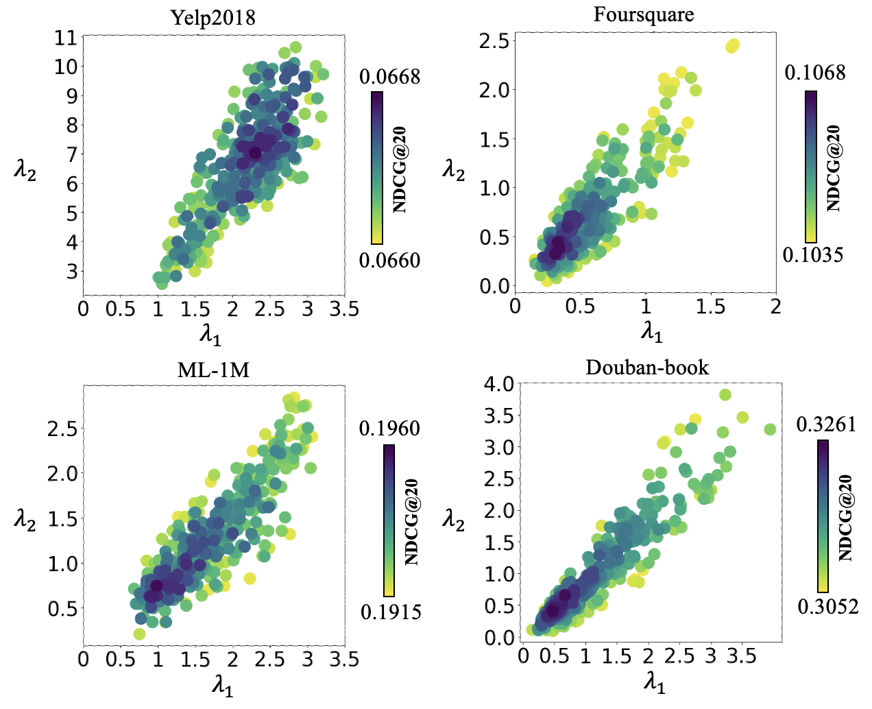
5.4.4. Effect of Weighting Scheme
Fig. 6 illustrates how the weighting scheme affects the CaDRec. We can see that various weighting schemes to balance embedding gradients of IA and FIA items significantly influence the quality of recommendations. We can also observe that (1) it suggests an optimal linear dependency between the optimal and , making it easier to seek the optimal solution when deploying a new dataset, and (2) the scaling coefficient affects the performance because even if values of and are close to the optimal linear region, their scaling still affects the recommendation quality of four datasets.
5.4.5. Study of Hyperparameter Sensitivity
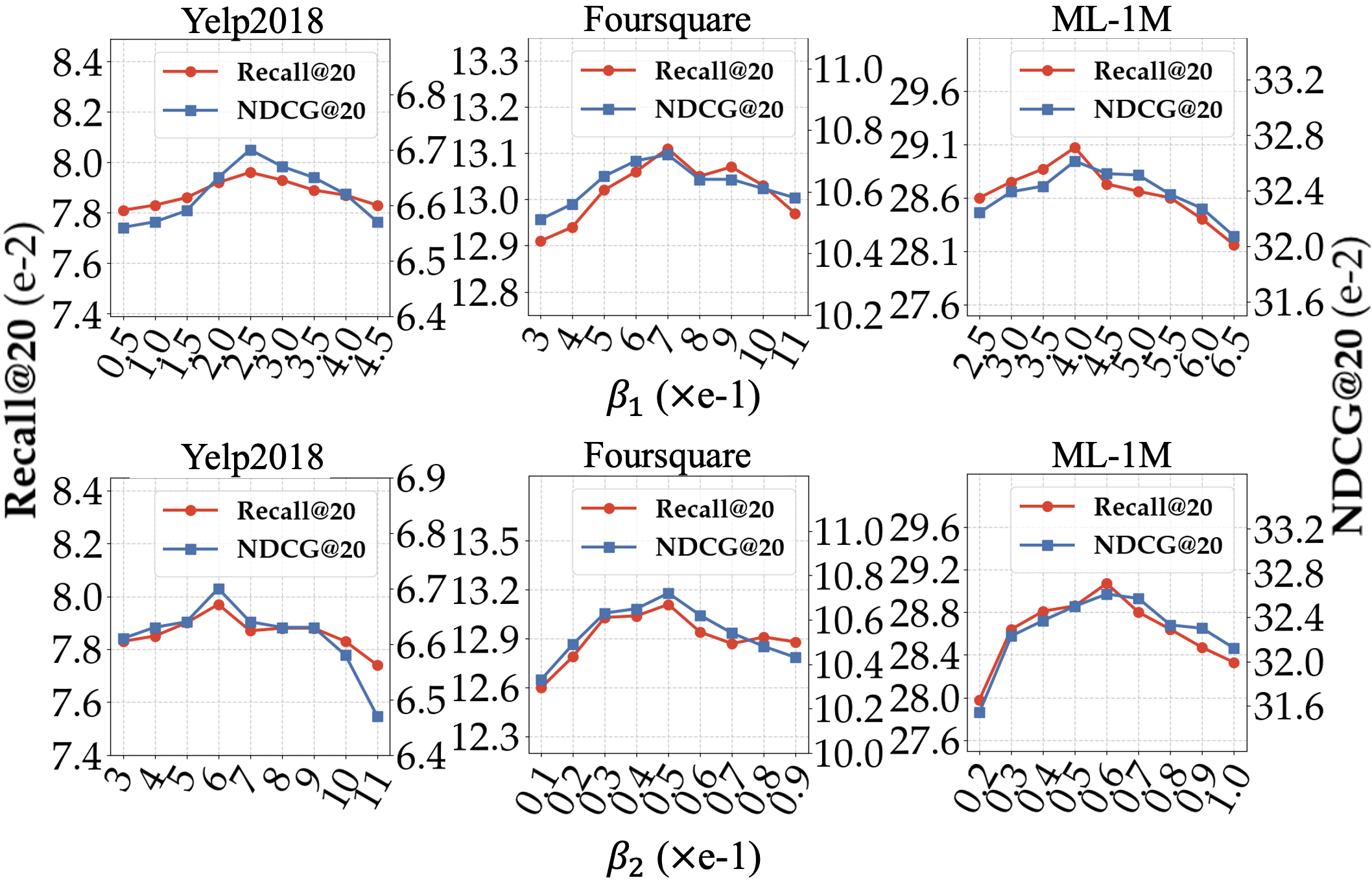
In this part, we investigate the impact of two key hyperparameters, i.e., and , in CaDRec. Due to the limited space, we only report the results on the Yelp2018, Foursquare, and ML-1M datasets, and the observations on the Douban-book dataset are similar.
Effect of . The hyperparameter of was assigned to vary the influence level of popularity. We can see from Fig. 7 that the best values of are 0.25 for Yelp2018, 0.7 for Foursquare, and 0.4 for ML-1M, respectively. Overall, the sensitivity of depends on the datasets, as there is no significant fluctuation by R@20 and N@20 on Yelp2018 and Foursquare datasets compared to the ML-1M dataset.
Effect of . The hyperparameter of is to control the penalization level of the L2 regularization. Fig. 7 shows that the best values of are 0.6 for Yelp2018, 0.05 for Foursquare, and 0.06 for ML-1M, respectively. We can conclude that a large average number of user interactions, for example, 68.2 in Foursquare and 95.3 in ML-1M, requires a small value of because more item embeddings are penalized in each iteration.
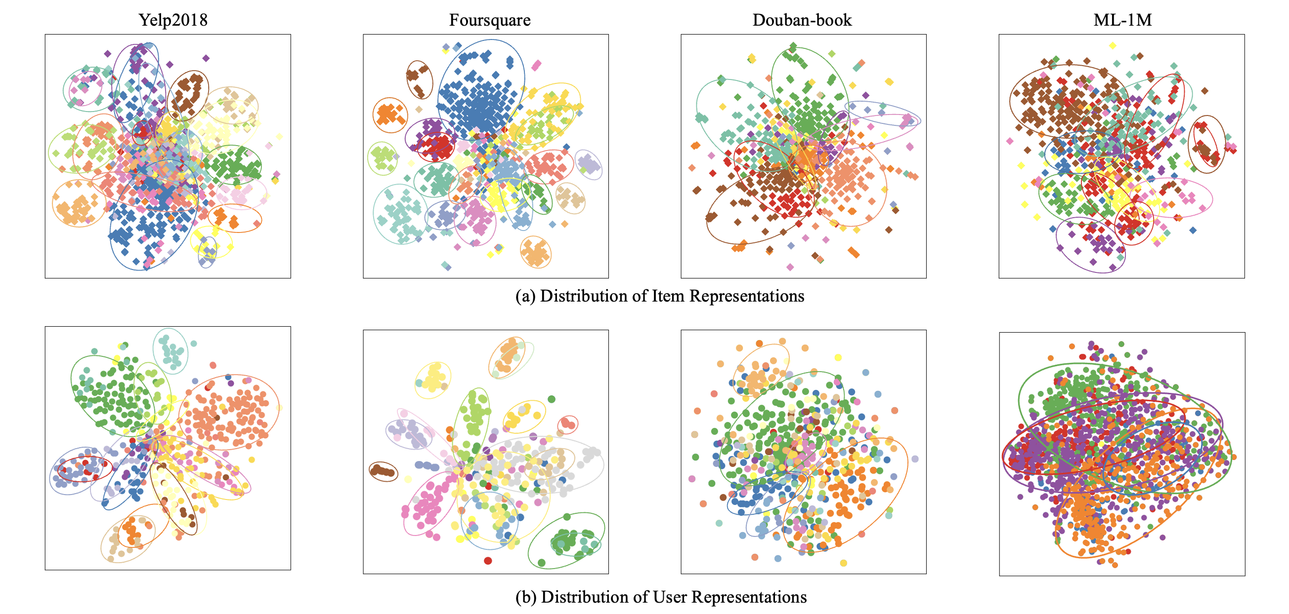
5.4.6. Visualization of User and Item Representations
To verify the effectiveness of the CaDRec, we visualized distributions of user and item representations learned by the CaDRec using t-SNE (Van der Maaten and Hinton, 2008), as illustrated in Fig. 8. We have the following observations:
-
•
Overall, the dots in the same color are close to each other, indicating that the CaDRec effectively differentiates similar users and items through learning contextualized and debiased representations from user–item interactions.
- •
-
•
Surprisingly, the visualization result on the ML-1M dataset is worse than the others, while Table 2 shows that the CaDRec works well on this dataset. The reason is that most users have interacted with many of the same items in the dataset according to the average interaction count in Table 1, leading to their representations sticking together in the 2D semantic space.
5.4.7. Time Complexity
We selected the top three baselines to compare the time complexity which highlights the efficiency of the CaDRec against the three baselines. We have the following observations and insights: (1) XSimGCL and NCL regard users and items as equivalent nodes in GCN which result in the complexity of , while that of HGC by the CaDRec is , where ; (2) the BPR loss () of XSimGCL and NCL uses negative samples to train each interaction of users, while the CaDRec learns all interactions of a user at a time; (3) XSimGCL and NCL regard the other samples in the same batch as negative samples for contrastive learning (); and (4) EEDN utilizes a stack of Transformers () in its decoder to capture implicit features. This leads to an additional exponential increase in time complexity for compared to CaDRec.
| Component | XSimGCL | NCL | EEDN | CaDRec |
|---|---|---|---|---|
| Encoder | ||||
| Decoder | ||||
| Obj. Loss | ||||
| CL Loss | - | - |
6. Conclusion
We proposed a CaDRec for a recommendation that integrates HGCs and Transformers to mitigate the over-smoothing issue and disentangle user–item interactions for debiasing. We also showed that the imbalance of the gradients for updating item embeddings magnifies the popularity bias and provides solutions. Extensive experiments and analyses have demonstrated the efficacy and efficiency of our CaDRec. In the future, we will (i) explore more effective ways to balance the gradients for updating item embeddings, and (ii) extend the CaDRec to automatically exclude ineffective contexts such as sequential contexts on the ML-1M dataset.
Acknowledgements
We would like to thank anonymous reviewers for their thorough comments. This work is supported by NEC C&C (No.24-004), China Scholarship Council (No.202208330093), and JKA (No.2023M-401).
References
- (1)
- Cai et al. (2023) Xuheng Cai, Chao Huang, Lianghao Xia, and Xubin Ren. 2023. LightGCL: Simple Yet Effective Graph Contrastive Learning for Recommendation. In The Eleventh International Conference on Learning Representations.
- Cao et al. (2022) Jiangxia Cao, Xixun Lin, Xin Cong, Jing Ya, Tingwen Liu, and Bin Wang. 2022. DisenCDR: Learning Disentangled Representations for Cross-Domain Recommendation. In Proceedings of the 45th International ACM SIGIR Conference on Research and Development in Information Retrieval. 267–277.
- Chen et al. (2021) Jiawei Chen, Xiang Wang, Fuli Feng, and Xiangnan He. 2021. Bias Issues and Solutions in Recommender System: Tutorial on the RecSys 2021. In Fifteenth ACM Conference on Recommender Systems. 825–827.
- Chen et al. (2022a) Lei Chen, Jie Cao, Youquan Wang, Weichao Liang, and Guixiang Zhu. 2022a. Multi-view graph attention network for travel recommendation. Expert Systems with Applications 191 (2022), 116234.
- Chen et al. (2022b) Zhihong Chen, Jiawei Wu, Chenliang Li, Jingxu Chen, Rong Xiao, and Binqiang Zhao. 2022b. Co-training Disentangled Domain Adaptation Network for Leveraging Popularity Bias in Recommenders. In Proceedings of the 45th International ACM SIGIR Conference on Research and Development in Information Retrieval. 60–69.
- Ding et al. (2022) Sihao Ding, Peng Wu, Fuli Feng, Yitong Wang, Xiangnan He, Yong Liao, and Yongdong Zhang. 2022. Addressing unmeasured confounder for recommendation with sensitivity analysis. In Proceedings of the 28th ACM SIGKDD Conference on Knowledge Discovery and Data Mining. 305–315.
- Goodfellow et al. (2014) Ian J Goodfellow, Jonathon Shlens, and Christian Szegedy. 2014. Explaining and harnessing adversarial examples. arXiv preprint arXiv:1412.6572 (2014).
- Hao et al. (2021) Bowen Hao, Jing Zhang, Hongzhi Yin, Cuiping Li, and Hong Chen. 2021. Pre-training graph neural networks for cold-start users and items representation. In Proceedings of the 14th ACM International Conference on Web Search and Data Mining. 265–273.
- He et al. (2020) Xiangnan He, Kuan Deng, Xiang Wang, Yan Li, Yongdong Zhang, and Meng Wang. 2020. Lightgcn: Simplifying and powering graph convolution network for recommendation. In Proceedings of the 43rd International ACM SIGIR conference on research and development in Information Retrieval. 639–648.
- He et al. (2022) Yue He, Zimu Wang, Peng Cui, Hao Zou, Yafeng Zhang, Qiang Cui, and Yong Jiang. 2022. Causpref: Causal preference learning for out-of-distribution recommendation. In Proceedings of the ACM Web Conference 2022. 410–421.
- Huang et al. (2022) Pei Huang, Yuting Yang, Fuqi Jia, Minghao Liu, Feifei Ma, and Jian Zhang. 2022. Word level robustness enhancement: Fight perturbation with perturbation. In Proceedings of the AAAI Conference on Artificial Intelligence, Vol. 36. 10785–10793.
- Keriven (2022) Nicolas Keriven. 2022. Not too little, not too much: a theoretical analysis of graph (over) smoothing. Advances in Neural Information Processing Systems 35 (2022), 2268–2281.
- Li et al. (2023) Qian Li, Xiangmeng Wang, Zhichao Wang, and Guandong Xu. 2023. Be causal: De-biasing social network confounding in recommendation. ACM Transactions on Knowledge Discovery from Data 17, 1 (2023), 1–23.
- Li et al. (2021) Yunqi Li, Hanxiong Chen, Shuyuan Xu, Yingqiang Ge, and Yongfeng Zhang. 2021. Towards personalized fairness based on causal notion. In Proceedings of the 44th International ACM SIGIR Conference on Research and Development in Information Retrieval. 1054–1063.
- Lin et al. (2022) Zihan Lin, Changxin Tian, Yupeng Hou, and Wayne Xin Zhao. 2022. Improving Graph Collaborative Filtering with Neighborhood-enriched Contrastive Learning. In Proceedings of the ACM Web Conference 2022. 2320–2329.
- Liu et al. (2021a) Dugang Liu, Pengxiang Cheng, Hong Zhu, Zhenhua Dong, Xiuqiang He, Weike Pan, and Zhong Ming. 2021a. Mitigating confounding bias in recommendation via information bottleneck. In Proceedings of the 15th ACM Conference on Recommender Systems. 351–360.
- Liu et al. (2023) Dugang Liu, Pengxiang Cheng, Hong Zhu, Zhenhua Dong, Xiuqiang He, Weike Pan, and Zhong Ming. 2023. Debiased representation learning in recommendation via information bottleneck. ACM Transactions on Recommender Systems 1, 1 (2023), 1–27.
- Liu et al. (2021b) Fan Liu, Zhiyong Cheng, Lei Zhu, Zan Gao, and Liqiang Nie. 2021b. Interest-aware message-passing gcn for recommendation. In Proceedings of the Web Conference 2021. 1296–1305.
- Ma et al. (2018) Chen Ma, Yingxue Zhang, Qinglong Wang, and Xue Liu. 2018. Point-of-interest recommendation: Exploiting self-attentive autoencoders with neighbor-aware influence. In Proceedings of the 27th ACM international conference on information and knowledge management. 697–706.
- Peng et al. (2022) Shaowen Peng, Kazunari Sugiyama, and Tsunenori Mine. 2022. Less is more: reweighting important spectral graph features for recommendation. In Proceedings of the 45th International ACM SIGIR Conference on Research and Development in Information Retrieval. 1273–1282.
- Qiu et al. (2022) Ruihong Qiu, Zi Huang, Hongzhi Yin, and Zijian Wang. 2022. Contrastive learning for representation degeneration problem in sequential recommendation. In Proceedings of the fifteenth ACM international conference on web search and data mining. 813–823.
- Ren et al. (2022) Weijieying Ren, Lei Wang, Kunpeng Liu, Ruocheng Guo, Lim Ee Peng, and Yanjie Fu. 2022. Mitigating popularity bias in recommendation with unbalanced interactions: A gradient perspective. In 2022 IEEE International Conference on Data Mining (ICDM). IEEE, 438–447.
- Rendle et al. (2012) Steffen Rendle, Christoph Freudenthaler, Zeno Gantner, and Lars Schmidt-Thieme. 2012. BPR: Bayesian personalized ranking from implicit feedback. arXiv preprint arXiv:1205.2618 (2012).
- Song et al. (2023) Zifan Song, Xiao Gong, Guosheng Hu, and Cairong Zhao. 2023. Deep perturbation learning: enhancing the network performance via image perturbations. In International Conference on Machine Learning. PMLR, 32273–32287.
- Tao et al. (2022) Wanjie Tao, Yu Li, Liangyue Li, Zulong Chen, Hong Wen, Peilin Chen, Tingting Liang, and Quan Lu. 2022. SMINet: State-Aware Multi-Aspect Interests Representation Network for Cold-Start Users Recommendation. In Proceedings of the AAAI Conference on Artificial Intelligence, Vol. 36. 8476–8484.
- Van der Maaten and Hinton (2008) Laurens Van der Maaten and Geoffrey Hinton. 2008. Visualizing data using t-SNE. Journal of machine learning research 9, 11 (2008).
- Vaswani et al. (2017) Ashish Vaswani, Noam Shazeer, Niki Parmar, Jakob Uszkoreit, Llion Jones, Aidan N Gomez, Łukasz Kaiser, and Illia Polosukhin. 2017. Attention is all you need. Advances in neural information processing systems 30 (2017).
- Wang et al. (2022) Chenyang Wang, Yuanqing Yu, Weizhi Ma, Min Zhang, Chong Chen, Yiqun Liu, and Shaoping Ma. 2022. Towards Representation Alignment and Uniformity in Collaborative Filtering. In Proceedings of the 28th ACM SIGKDD Conference on Knowledge Discovery and Data Mining. 1816–1825.
- Wang et al. (2023d) Wenjie Wang, Yiyan Xu, Fuli Feng, Xinyu Lin, Xiangnan He, and Tat-Seng Chua. 2023d. Diffusion Recommender Model. In Proceedings of the 46th International ACM SIGIR Conference on Research and Development in Information Retrieval. 832–841.
- Wang et al. (2023a) Xinfeng Wang, Fumiyo Fukumoto, Jin Cui, Yoshimi Suzuki, Jiyi Li, and Dongjin Yu. 2023a. EEDN: Enhanced Encoder-Decoder Network with Local and Global Interactions for POI Recommendation. In Proceedings of the 46th International ACM SIGIR Conference on Research and Development in Information Retrieval. 383–392.
- Wang et al. (2023b) Xinfeng Wang, Fumiyo Fukumoto, Jiyi Li, Dongjin Yu, and Xiaoxiao Sun. 2023b. STaTRL: Spatial-temporal and text representation learning for POI recommendation. Applied Intelligence 53, 7 (2023), 8286–8301.
- Wang et al. (2023c) Yifan Wang, Weizhi Ma, Min Zhang, Yiqun Liu, and Shaoping Ma. 2023c. A survey on the fairness of recommender systems. ACM Transactions on Information Systems 41, 3 (2023), 1–43.
- Wu et al. (2021) Jiancan Wu, Xiang Wang, Fuli Feng, Xiangnan He, Liang Chen, Jianxun Lian, and Xing Xie. 2021. Self-supervised graph learning for recommendation. In Proceedings of the 44th international ACM SIGIR conference on research and development in information retrieval. 726–735.
- Wu et al. (2019) Qiong Wu, Yong Liu, Chunyan Miao, Binqiang Zhao, Yin Zhao, and Lu Guan. 2019. PD-GAN: Adversarial learning for personalized diversity-promoting recommendation.. In IJCAI, Vol. 19. 3870–3876.
- Xia et al. (2023) Lianghao Xia, Chao Huang, Chunzhen Huang, Kangyi Lin, Tao Yu, and Ben Kao. 2023. Automated Self-Supervised Learning for Recommendation. In Proceedings of the ACM Web Conference 2023. 992–1002.
- Xia et al. (2022b) Lianghao Xia, Chao Huang, Yong Xu, Jiashu Zhao, Dawei Yin, and Jimmy Huang. 2022b. Hypergraph contrastive collaborative filtering. In Proceedings of the 45th International ACM SIGIR conference on research and development in information retrieval. 70–79.
- Xia et al. (2022a) Lianghao Xia, Chao Huang, and Chuxu Zhang. 2022a. Self-supervised hypergraph transformer for recommender systems. In Proceedings of the 28th ACM SIGKDD Conference on Knowledge Discovery and Data Mining. 2100–2109.
- Xiao et al. (2022) Teng Xiao, Zhengyu Chen, and Suhang Wang. 2022. Representation Matters When Learning From Biased Feedback in Recommendation. In Proceedings of the 31st ACM International Conference on Information & Knowledge Management. 2220–2229.
- Yan et al. (2023) Xiaodong Yan, Tengwei Song, Yifeng Jiao, Jianshan He, Jiaotuan Wang, Ruopeng Li, and Wei Chu. 2023. Spatio-temporal hypergraph learning for next POI recommendation. In Proceedings of the 46th International ACM SIGIR Conference on Research and Development in Information Retrieval. 403–412.
- Yu et al. (2023) Junliang Yu, Xin Xia, Tong Chen, Lizhen Cui, Nguyen Quoc Viet Hung, and Hongzhi Yin. 2023. XSimGCL: Towards extremely simple graph contrastive learning for recommendation. IEEE Transactions on Knowledge and Data Engineering (2023).
- Yu et al. (2021a) Junliang Yu, Hongzhi Yin, Min Gao, Xin Xia, Xiangliang Zhang, and Nguyen Quoc Viet Hung. 2021a. Socially-aware self-supervised tri-training for recommendation. In Proceedings of the 27th ACM SIGKDD Conference on Knowledge Discovery & Data Mining. 2084–2092.
- Yu et al. (2021b) Junliang Yu, Hongzhi Yin, Jundong Li, Qinyong Wang, Nguyen Quoc Viet Hung, and Xiangliang Zhang. 2021b. Self-supervised multi-channel hypergraph convolutional network for social recommendation. In Proceedings of the Web Conference 2021. 413–424.
- Yu et al. (2022a) Junliang Yu, Hongzhi Yin, Xin Xia, Tong Chen, Lizhen Cui, and Quoc Viet Hung Nguyen. 2022a. Are graph augmentations necessary? simple graph contrastive learning for recommendation. In Proceedings of the 45th International ACM SIGIR Conference on Research and Development in Information Retrieval. 1294–1303.
- Yu et al. (2022b) Wenhui Yu, Zixin Zhang, and Zheng Qin. 2022b. Low-Pass Graph Convolutional Network for Recommendation. In Proceedings of the AAAI Conference on Artificial Intelligence, Vol. 36. 8954–8961.
- Zhang et al. (2022) An Zhang, Wenchang Ma, Xiang Wang, and Tat-Seng Chua. 2022. Incorporating Bias-aware Margins into Contrastive Loss for Collaborative Filtering. In Advances in Neural Information Processing Systems, Vol. 35. 7866–7878.
- Zhang et al. (2023b) An Zhang, Jingnan Zheng, Xiang Wang, Yancheng Yuan, and Tat-Seng Chua. 2023b. Invariant Collaborative Filtering to Popularity Distribution Shift. In Proceedings of the ACM Web Conference 2023. 1240–1251.
- Zhang et al. (2023a) Jingsen Zhang, Xu Chen, Jiakai Tang, Weiqi Shao, Quanyu Dai, Zhenhua Dong, and Rui Zhang. 2023a. Recommendation with Causality enhanced Natural Language Explanations. In Proceedings of the ACM Web Conference 2023. 876–886.
- Zhang et al. (2024) Yifei Zhang, Hao Zhu, Zixing Song, Piotr Koniusz, Irwin King, et al. 2024. Mitigating the Popularity Bias of Graph Collaborative Filtering: A Dimensional Collapse Perspective. Advances in Neural Information Processing Systems 36 (2024).
- Zhao et al. (2022) Zihao Zhao, Jiawei Chen, Sheng Zhou, Xiangnan He, Xuezhi Cao, Fuzheng Zhang, and Wei Wu. 2022. Popularity Bias Is Not Always Evil: Disentangling Benign and Harmful Bias for Recommendation. IEEE Transactions on Knowledge & Data Engineering 01 (2022), 1–13.
- Zheng et al. (2021) Yu Zheng, Chen Gao, Xiang Li, Xiangnan He, Yong Li, and Depeng Jin. 2021. Disentangling user interest and conformity for recommendation with causal embedding. In Proceedings of the Web Conference 2021. 2980–2991.
- Zhou et al. (2023) Huachi Zhou, Hao Chen, Junnan Dong, Daochen Zha, Chuang Zhou, and Xiao Huang. 2023. Adaptive Popularity Debiasing Aggregator for Graph Collaborative Filtering. In Proceedings of the 46th International ACM SIGIR Conference on Research and Development in Information Retrieval. 7–17.