Impact of reflection Comptonization on X-ray reflection spectroscopy:
the case of EXO 1846–031

Abstract

Within the disk-corona model, it is natural to expect that a fraction of reflection photons from the disk are Compton scattered by the hot corona (reflection Comptonization), even if this effect is usually ignored in X-ray reflection spectroscopy studies. We study the effect by using NICER and NuSTAR data of the Galactic black hole EXO 1846–031 in the hard-intermediate state with the model simplcutx. Our analysis suggests that a scattered fraction of order 10% is required to fit the data, but the inclusion of reflection Comptonization does not change appreciably the measurements of key-parameters like the black hole spin and the inclination angle of the disk.

I Introduction

In the disk-corona model, a black hole accretes from a geometrically thin and optically thick accretion disk, as shown in Fig. 1 Bambi et al. (2021); Fabian et al. (1995); Zoghbi et al. (2010); Risaliti et al. (2013). The disk can be described by the Novikov-Thorne model Novikov and Thorne (1973) and has a multicolor blackbody spectrum. A portion of the thermal photons are subsequently scattered by hot electrons residing in the corona, yielding a power-law component in the spectrum. The power-law component illuminates the disk, thereby producing a reflection component marked by fluorescent emission lines in the soft X-ray band and a Compton hump with a peak at 20-30 keV Ross and Fabian (2005); García and Kallman (2010). With high quality data and the correct astrophysical model, X-ray reflection spectroscopy can be a powerful tool to study the morphology of the accreting system and the spacetime around the black hole (Bambi et al., 2021).

The corona plays a vital role in the process of spectrum generation within this paradigm. In the Comptonization of photons emitted from the accretion disk, we often consider Comptonization of thermal photons from the disk, ignoring the reflection photons. Reflection photons should also undergo Compton scattering off electrons in the corona above the accretion disk Steiner et al. (2016, 2017), as shown in Fig. 1 by the magenta arrow. Such a reflection Comptonization seems to be unavoidable, but it is normally overlooked in the spectral analysis of accreting black holes. Wilkins and Gallo (2015) showed that an extended corona in active galactic nuclei (AGN) should scatter the reflection photons and a similar conclusion can be expected in the case of stellar-mass black holes in X-ray binary systems. The fraction of reflection photons that are Compton scattered by the corona should depend on the extension of the corona and its optical depth. If the corona covers a sufficiently large fraction of the inner part of the accretion disk and its optical depth is not low, the reflection Comptonization is expected to have an impact on the spectral analysis and on the estimates of the properties of the accreting system.

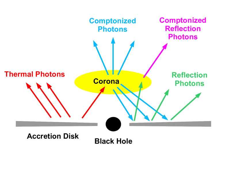
Figure 1: Disk-corona system with reflection Comptonization.

In this paper, we present a study of the impact of the reflection Comptonization on the analysis of a reflection dominated spectrum of a Galactic black hole, EXO 1846–031. We use simplcutx Steiner et al. (2017) to describe any Compton scattering in the corona. We compare the measurements of the properties of the spectrum with and without including the effect of reflection Comptonization.

EXO 1846–031 is a black hole X-ray binary discovered by EXOSAT on April 3, 1985 (Parmar and White, 1985). After a quiescent period of over two decades, it experienced a new outburst in 2019, which was first detected by MAXI/GSC on July 23, 2019 Negoro et al. (2019). This outburst was also observed by other missions during the following few weeks, such as Swift Mereminskiy et al. (2019), NICER (Bult et al., 2019), and NuSTAR Miller et al. (2019). During the hard to soft state transition (Yang et al., 2019a), the source showed a spectrum with strong reflection features Miller et al. (2019) and quasi-periodic oscillations (QPOs) (Yang et al., 2019b). Draghis et al. (2020) found that the black hole in EXO 1846–031 has a spin parameter very close to 1 and the viewing angle of its accretion disk is high, close to 70 deg. Thanks to the very strong reflection features in the NuSTAR spectrum, this source has been widely used to test new reflection models (see, e.g., Refs. Abdikamalov et al. (2021); Tripathi et al. (2021a)) as well as different spacetime metrics from modified gravity theories (see, e.g., Refs. Tripathi et al. (2021b); Yu et al. (2021); Gu et al. (2022); Tao et al. (2023)). Abdikamalov et al. (2021) showed that a radial disk ionization profile can improve the fit of the spectrum around 7 keV. QPOs were studied in Liu et al. (2021) and the possible existence of a disk wind was studied in Wang et al. (2021).

Past studies have shown that EXO 1846–031 exhibits strong reflection features. In the present manuscript, we still analyze the NuSTAR spectrum of the 2019 outburst, but we also incorporate soft X-ray data from NICER and perform joint fitting analysis to explore whether this will lead to any differences in the final results.

The content of the manuscript is as follows. In Section II, we present the observation information and data reduction process. In Section III, we describe the two model configurations to study the impact of reflection Comptonization and present the spectral analysis results of the observation of EXO 1846–031. We discuss our results in Section IV and present our conclusions in Section V.

II Observations and data reduction

EXO 1846–031 was observed by NuSTAR and NICER on August 3, 2019. The source was in a transitional phase from hard state to intermediate state (Ren et al., 2022). The X-ray flux was about 46% of the soft state peak (see Fig. 2). The details of the observations analyzed in our work are shown in Table 1.

Table 1: List of the observations analyzed in this paper.

	Source	Mission	Observation ID	Observation Time	Exposure (ks)	Count rate ($\rm s^{-1}$)
	EXO 1846–031	NuSTAR	90501334002	2019-08-03 02:01:09	22.2	148.7
		NICER	2200760104	2019-08-03 02:08:58	0.911	376.1

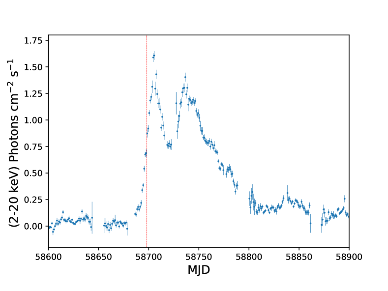
Figure 2: Light curve of EXO 1846–031 from Monitor of All-sky X-ray Image (MAXI). The red-dashed line marks the observation date of the data we used.

For the NuSTAR observation, we reduced the data with NuSTARDAS and the CALDB 20220301 (Madsen et al., 2022). We selected a circular region with a radius of $180^{\prime\prime}$ on both focal plane module A (FPMA) and focal plane module B (FPMB) detectors to extract the source spectra. In order to prevent influence from the source photons, a background region of comparable size was selected far from the source region. Afterwards, we used nuproducts to generate the source and background spectra. We grouped the spectra with the optimal binning algorithm in Kaastra and Bleeker (2016) by using the ftgrouppha task.

For the NICER observation, the NICERDAS software suite was used to process the data. Extractions used standard screenings for the Sun angle, bright-Earth limb, and boresight. Any South Atlantic Anomaly (SAA) passages were excised. Data from detectors 14, 34, and 54, were screened out, owing to intermittent calibration issues manifest from those detectors. All other of NICER’s 49 additional working detectors were on, and from this set of events the detector ensemble distribution of X-ray events, undershoots, and overshoots were separately compared. There were no significant outliers, and so the remaining 49 active detectors were all used for spectral extraction. Undershoot levels were low for the observation in question, which ensures the robustness of the gain solution. The spectrum was adaptively binned to oversample the instrumental resolution by a factor of 2-3, and include at least 5 counts per bin. The 3C50 background model (Remillard et al., 2022) was used to produce background spectra.

III Data Analysis

We use XSPEC v12.12.1 (Arnaud, 1996) to analyze the spectra. We use two different datasets for the spectral fitting process: the spectra from NuSTAR only (our “NuSTAR data”), and the spectra from both NuSTAR and NICER (our “NuSTAR+NICER data”) for a joint fitting. The reason is to demonstrate the influence of soft X-ray data on the fitting. The fits are made across the 3.0-79.0 keV energy band of NuSTAR and the 1.0-10.0 keV energy band for NICER. In the joint fitting of NuSTAR and NICER data, NuSTAR data below 4.5 keV are ignored in order to avoid the mismatch between NICER and NuSTAR at the low energy band, as demonstrated by other studies (Tao et al., 2019; Nath et al., 2024).

Firstly, we fit the data with an absorbed disk black-body and power-law to see the reflection features in the spectrum. In XSPEC language, the model reads

$${\tt tbabs}*({\tt diskbb}+{\tt nthcomp}),$$ (1)

where tbabs describes the galactic absorption with the abundance table from Wilms et al. (2000), diskbb (Pringle, 1981; Mitsuda et al., 1984) describes the thermal component, and nthcomp (Zdziarski et al., 1996; Życki et al., 1999) describes the power-law component. We link $T_{\rm in}$ in diskbb to $T_{\rm bb}$ in nthcomp. We clearly see reflection features with an a broad iron line around 7 keV and a Compton hump peaking around 20-30 keV (Fig. 3).

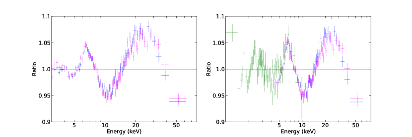
Figure 3: Data to best-fit model ratio plots for an absorbed disk blackbody and power-law model. The left panel is for NuSTAR data and the right panel is for NuSTAR+NICER data. The blue and purple crosses are for the FPMA/NuSTAR and FPMB/NuSTAR data and the green crosses are for the NICER data.

III.1 Model 1: conventional modeling

Previous study on the same observation shows that a reflection model that assumes a radial ionization gradient can fit the data better (Abdikamalov et al., 2021). Therefore, we implement the relxillion_nk model which describes the ionization profile with a power-law:

$$\xi(r)=\xi_{0}\left(\frac{R_{\rm in}}{r}\right)^{\alpha_{\xi}},$$ (2)

where $\xi_{0}$ is the value of the ionization parameter at the inner edge of the disk, $R_{\rm in}$ is the radial coordinate of the inner edge of the disk, and $\alpha_{\xi}$ is the index of the power-law ionization profile. The total model is tbabs*(diskbb+nthcomp+relxillionCp_nk) (Model 1), where relxillionCp_nk is a flavor of relxillion_nk that uses the nthcomp Comptonization continuum for the incident spectrum.

III.2 Model 2: self-consistent modeling with simplcutx

Adopting a more self-consistent model structure, the power-law component is generated from Comptonization of the thermal component in the corona, and the reflection component originating from the disk surface will also be Comptonized (Steiner et al., 2017). In XSPEC language, the model expression is tbabs*simplcutx*(diskbb+relxillionCp_nk) (Model 2). We set the reflection fraction $R_{\rm F}$ in simplcutx as 1 to avoid parameter degeneracy. In simplcutx, $R_{\rm F}$ is defined as the number of scattered photons that return to illuminate the disk divided by the number of photons that reach infinity.

III.3 Analysis for the emissivity profile

The emissivity profile depends on the geometry of the corona, which is unknown. Therefore, we model the emissivity profile using an empirical broken power-law ($\epsilon\propto 1/r^{q_{\rm in}}$ for $r<R_{\rm break}$, $\epsilon\propto 1/r^{q_{\rm out}}$ for $r>R_{\rm break}$). In previous studies on EXO 1846–031 (Draghis et al., 2020; Abdikamalov et al., 2021), the authors found that the NuSTAR data can be fit well with a broken power-law emissivity profile with a high inner emissivity index ($q_{\rm in}\approx 10$) and an almost flat emissivity profile ($q_{\rm out}\approx 0$) at larger radii. We note that the luminosity of an infinite disk is finite only if $q_{\rm out}>2$. Moreover, the theoretical reflection spectrum will obviously change with the variation of the disk’s outer radius $R_{\rm out}$ if $q_{\rm out}$ is close to zero in reflection models like relxill_nk. This means that in our case with $q_{\rm out}\approx 0$ the reflection spectrum does depend on the exact value of the outer radial coordinate of the disk (see Fig. 4 for an example).

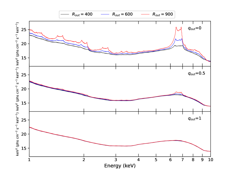
Figure 4: Relativistic reflection spectra with different values of $q_{\rm out}$ and $R_{\rm out}$. In all of these plots, the other parameters are set to the same specific values: $q_{\rm in}=10$, $R_{\rm br}=6~{}R_{\rm g}$, $R_{\rm in}=R_{\rm ISCO}$, $a_{*}=0.998$, $i=75^{\circ}$, $\Gamma=2$, $E_{\rm cut}=100$ keV, $\log\xi=3.1$, $A_{\rm Fe}=1$.

Since the maximum value of the outer radius of the disk in our reflection model is 900 gravitational radii ($R_{\rm g}$) and if we leave it free it seems like the fit requires a larger value than this, we consider three different scenarios: $q_{\rm out}$ is free (case A), $q_{\rm out}=3$ (case B), $q_{\rm out}$ is free and we add a distant reflector with xillverCp, in which the ionization parameter is low ($\log\xi=0$; case C). We set $R_{\rm out}$ to its maximum value in the model in order to be sensitive even to the radiation emitted at relatively large radii.

All models we tested are summarized in Table 2.

Table 2: Models used to analyze the NuSTAR data of EXO 1846–031. As for the NuSTAR+NICER data, we just replace constant with crabber*edge*xscat.

model	$q_{\rm out}$	XSPEC model for NuSTAR data
1A	free	constant*tbabs*(diskbb + nthcomp + relxillionCp_nk)
1B	$3^{*}$	constant*tbabs*(diskbb + nthcomp + relxillionCp_nk)
1C	free	constant*tbabs*(diskbb + nthcomp + relxillionCp_nk + xillverCp)
2A	free	constant*tbabs*simplcutx*(diskbb + relxillionCp_nk)
2B	$3^{*}$	constant*tbabs*simplcutx*(diskbb + relxillionCp_nk)
2C	free	constant*tbabs*(simplcutx*(diskbb + relxillionCp_nk)+xillverCp)

III.4 Other setting and final results

For the NuSTAR data, we only set a cross-calibration constant between FPMA and FPMB. For the NuSTAR+NICER data, we add an edge component to fit an absorption edge around 1.84 keV. We also apply the xscat model (Smith et al., 2016) for all data as the field of view of NICER is comparable to the typical size of a dust scattering halo. We choose the MRN dust model for the scattering. For the extraction regions, the radius is 50^′′ for the NuSTAR data and 180^′′ for the NICER data, in accordance with the configuration in Barillier et al. (2023). Furthermore, we apply a cross-calibration model called crabber (Steiner et al., 2010) which is designed to standardize the calibration parameters between different detectors for the Crab Nebula (power-law normalization and index) via a multiplicative power-law correction. All parameters in the NuSTAR and NICER spectra are linked except the cross-calibration parameters.

For both Model 1 and Model 2, we link $\Gamma$ and $kT_{e}$ between the power-law component (simplcutx or nthcomp) and the reflection component (relxillionCp_nk and xillverCp). The reflection fraction $R_{\rm f}$ in relxillionCp_nk is set to $-1$, so the model returns only the reflection component. We also link the neutral column in xscat to the value from tbabs.

We apply the AICc (Burnham, 1998), which is the Akaike information criterion (AIC) (Akaike, 1974) corrected for small sample sizes and provides a mean for selecting the best model among several model candidates. The model candidate with the lowest AICc is the best model. The formulas used to calculate AIC and AICc are

$${\rm AIC}=-2{\rm ln}\mathcal{L}+2N_{p}$$ (3)

and

$${\rm AICc}={\rm AIC}+2N_{p}(N_{p}+1)/(N_{b}-N_{p}-1),$$ (4)

where $N_{p}$ is the number of free parameters, $N_{b}$ is the number of bins and $\mathcal{L}$ is the likelihood of the best-fit model. The values of likelihood can be written in terms of $\chi^{2}$ which is obtained from the model’s best fit: $\chi^{2}=-2\ln\mathcal{L}$.

For the NuSTAR data, the best-fit for all models are presented in Table 3 and the best-fit model plots and residual plots are presented in Fig. 5.

Table 3: Best-fit values of all models with NuSTAR data. $P$ means that we reach the lower or upper limit of the model.

Model	Model 1A	Model 1B	Model 1C	Model 2A	Model 2B	Model 2C
tbabs
$N_{\rm H}$ [$10^{22}$ cm-2]	$7.7_{-0.5}^{+0.5}$	$9.7_{-0.6}^{+0.4}$	$7.66_{-0.21}^{+0.5}$	$7.7_{-0.6}^{+0.5}$	$10.5_{-0.5}^{+0.6}$	$7.7_{-0.4}^{+0.6}$
diskbb
$T_{\rm in}$	$0.33_{-0.04}^{+0.04}$	$0.452_{-0.011}^{+0.011}$	$0.33_{-0.06}^{+0.04}$	$0.349_{-0.014}^{+0.019}$	$0.459_{-0.004}^{+0.011}$	$0.337_{-0.015}^{+0.012}$
Norm	$1.1_{-0.6}^{+2.4}\times 10^{5}$	$1.88_{-0.4}^{+0.23}\times 10^{4}$	$1.1_{-0.6}^{+2.3}\times 10^{5}$	$8.6_{-1.8}^{+6}\times 10^{4}$	$2.48_{-0.4}^{+0.23}\times 10^{4}$	$1.13_{-0.11}^{+0.25}\times 10^{5}$
simplcutx
$\Gamma$				$2.139_{-0.014}^{+0.012}$	$1.9345_{-0.0026}^{+0.03}$	$2.14_{-0.02}^{+0.03}$
$kT_{\rm e}$ [keV]				$58.7_{-16.3}^{+9}$	$31.6_{-1.6}^{+1.8}$	$66_{-18.8}^{+30.0}$
$f_{\tt SC}$				$0.215_{-0.026}^{+0.013}$	$0.120_{-0.04}^{+0.024}$	$0.196_{-0.03}^{+0.015}$
nthcomp
$\Gamma$	$2.102_{-0.015}^{+0.028}$	$1.986_{-0.011}^{+0.007}$	$2.102_{-0.04}^{+0.024}$
$kT_{\rm e}$ [keV]	$61_{-17.8}^{+26.9}$	$31.1_{-2.1}^{+4}$	$61_{-20.7}^{+17.6}$
Norm	$1.70_{-0.13}^{+0.16}$	$1.12_{-0.13}^{+0.03}$	$1.70_{-0.14}^{+0.16}$
relxillionCp_nk
$q_{\rm in}$	$9.8_{-2.1}^{+P}$	$10.0_{-0.3}^{+P}$	$9.8_{-2.1}^{+P}$	$9.5_{-1.4}^{+0.4}$	$10.0_{-1.4}^{+P}$	$9.5_{-1.7}^{+0.5}$
$q_{\rm out}$	$0.17_{-P}^{+0.9}$	$3^{*}$	$0.17_{-P}^{+1.1}$	$0.0011_{-P}^{+1.1}$	$3^{*}$	$0.8_{-0.4}^{+0.3}$
$R_{\rm br}$ [$R_{\rm g}$]	$6.6_{-1.4}^{+2.9}$	$3.00_{-0.12}^{+0.29}$	$6.6_{-1.5}^{+1.0}$	$7.5_{-0.9}^{+1.2}$	$3.18_{-0.17}^{+0.4}$	$5.1_{-1.5}^{+1.7}$
$a_{*}$	$0.9912_{-0.0028}^{+0.0019}$	$0.973_{-0.016}^{+0.005}$	$0.9912_{-0.0026}^{+0.002}$	$0.9914_{-0.0022}^{+0.003}$	$0.953_{-0.024}^{+0.023}$	$0.9918_{-0.0027}^{+0.0022}$
$i$ [deg]	$76.5_{-1.5}^{+1.2}$	$67.7_{-2.7}^{+1.4}$	$76.5_{-0.5}^{+1.3}$	$76.4_{-0.6}^{+0.6}$	$62.7_{-2.4}^{+7}$	$76.8_{-0.6}^{+1.4}$
AFe	$0.88_{-0.15}^{+0.18}$	$2.20_{-0.5}^{+0.28}$	$0.88_{-0.08}^{+0.21}$	$0.91_{-0.17}^{+0.3}$	$10.0_{-1.3}^{+P}$	$0.88_{-0.06}^{+0.5}$
$\alpha_{\xi}$	$0.18_{-0.04}^{+0.05}$	$0.001_{-P}^{+0.08}$	$0.178_{-0.05}^{+0.019}$	$0.176_{-0.028}^{+0.026}$	$0.14_{-P}^{+0.16}$	$0.18_{-0.05}^{+0.04}$
log${\xi}$ [erg cm s-1]	$3.13_{-0.11}^{+0.18}$	$3.60_{-0.08}^{+0.1}$	$3.13_{-0.11}^{+0.12}$	$3.10_{-0.04}^{+0.12}$	$4.52_{-0.16}^{+0.04}$	$3.10_{-0.07}^{+0.19}$
Norm	$0.0061_{-0.0009}^{+0.0011}$	$0.0038_{-0.0003}^{+0.0003}$	$0.0061_{-0.0006}^{+0.001}$	$0.0083_{-0.0012}^{+0.0009}$	$0.00526_{-0.00024}^{+0.0008}$	$0.0083_{-0.0018}^{+0.0012}$
xillverCp
Norm			$0.0001_{-P}^{+0.004}$			$0.0012_{-P}^{+0.002}$
$C_{\rm FPMB}$	$1.0152_{-0.0014}^{+0.0014}$	$1.0152_{-0.0014}^{+0.0014}$	$1.0152_{-0.0014}^{+0.0014}$	$1.0152_{-0.0014}^{+0.0014}$	$1.0152_{-0.0014}^{+0.0014}$	$1.0152_{-0.0014}^{+0.0013}$
$\chi^{2}$ /dof	633.03/513	695.0/514	633.0/512	632.85/513	701.7/514	632.7/512
	=1.23398	=1.35214	=1.23633	=1.23363	=1.36518	=1.23574
AICc	666.09	725.94	668.2	665.91	732.64	667.9

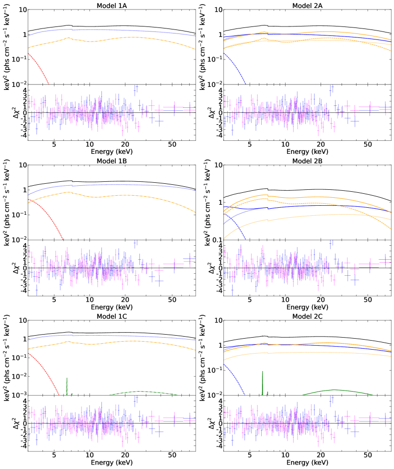
Figure 5: Model and residual plots for EXO 1846–031 with NuSTAR data. In the left panel, the red lines represent the thermal components, the blue lines represent the power-law components, and orange lines represent the reflection components. In the right panel, the blue lines represent the Comptonized thermal spectra, and the orange lines represent the Comptonized reflection spectra. For the lines with same color, solid lines represent the complete spectra, dotted lines represent the components scattered by the corona, and dashed lines represent the components transmitted by the corona.

As for the NuSTAR+NICER data, the best-fit for all models are presented in Table 4 and the best-fit model plots and residual plots are presented in Fig. 6. In addition, for all the plots of best-fit models with simplcutx, we also plot the scattered and transmitted spectra separately.

Table 4: Best-fit values and unabsorbed flux of all models with NuSTAR+NICER data. $P$ means that we reach the lower or upper limit of the model. In the estimate of the Eddington ratio (last row), $D$ is the distance in the unit of kpc and $M$ is the mass in the unit of $M_{\odot}$. The estimate of the total flux is obtained by integrating the total spectrum of the best-fit model from 0.01 to 1000 keV.

Model	Model 1A-1	Model 2A-1	Model 1A-2	Model 2A-2
edge
$\tau_{\tt max}$	$0.095_{-0.022}^{+0.026}$	$0.098_{-0.018}^{+0.015}$	$0.122_{-0.015}^{+0.016}$	$0.115_{-0.014}^{+0.024}$
tbabs
$N_{\rm H}$ [$10^{22}$ cm-2]	$6.33_{-0.1}^{+0.09}$	$6.48_{-0.11}^{+0.11}$	$5.60_{-0.05}^{+0.29}$	$5.82_{-0.19}^{+0.07}$
xscat
$x$	$1.00_{-0.05}^{+P}$	$1.00_{-0.05}^{+P}$	$0.90_{-0.12}^{+0.08}$	$0.99_{-0.13}^{+P}$
diskbb
$T_{\rm in}$	$0.192_{-0.01}^{+0.008}$	$0.202_{-0.01}^{+0.006}$	$0.42_{-0.06}^{+0.03}$	$0.40_{-0.09}^{+0.04}$
Norm	$6.2_{-2.7}^{+2.8}\times 10^{5}$	$7.59_{-0.04}^{+4}\times 10^{5}$	$1098_{-668}^{+2152}$	$1875_{-1156}^{+2723}$
simplcutx
$\Gamma$		$2.098_{-0.007}^{+0.017}$		$1.907_{-0.007}^{+0.023}$
$kT_{\rm e}$ [keV]		$44.3_{-5}^{+1.4}$		$36.1_{-1.8}^{+6}$
$f_{\tt SC}$		$0.229_{-0.028}^{+0.08}$		$0.150_{-0.04}^{+0.021}$
nthcomp
$\Gamma$	$2.052_{-0.004}^{+0.026}$		$1.875_{-0.007}^{+0.007}$
$kT_{\rm e}$ [keV]	$38.0_{-2.5}^{+1.6}$		$41.4_{-1.8}^{+1.2}$
Norm	$1.935_{-0.012}^{+0.018}$		$0.376_{-0.015}^{+0.14}$
relxillionCp_nk
$q_{\rm in}$	$10.0_{-1.4}^{+P}$	$10.00_{-0.22}^{+P}$	$9.8_{-0.9}^{+P}$	$9.9_{-0.7}^{+P}$
$q_{\rm out}$	$0.46_{-0.12}^{+0.6}$	$0.52_{-0.09}^{+0.15}$	$1.44_{-0.26}^{+0.08}$	$1.259_{-0.5}^{+0.028}$
$R_{\rm br}$ [$R_{\rm g}$]	$5.59_{-0.26}^{+0.2}$	$5.5_{-0.3}^{+0.8}$	$4.45_{-0.29}^{+0.8}$	$5.10_{-0.6}^{+0.13}$
$a_{*}$	$0.9912_{-0.0025}^{+0.0015}$	$0.990_{-0.002}^{+0.004}$	$0.9851_{-0.004}^{+0.0017}$	$0.978_{-0.002}^{+0.007}$
$i$ [deg]	$75.9_{-1.3}^{+0.7}$	$75.1_{-1.3}^{+1.3}$	$68.98_{-6}^{+0.27}$	$68.4_{-0.4}^{+0.6}$
AFe	$1.40_{-0.3}^{+0.19}$	$0.867_{-0.016}^{+0.1}$	$7.5_{-1.0}^{+0.3}$	$6.60_{-1.8}^{+0.26}$
$\alpha_{\xi}$	$0.179_{-0.026}^{+0.04}$	$0.204_{-0.012}^{+0.04}$	$1.11_{-0.21}^{+0.5}$	$1.03_{-0.3}^{+0.24}$
log${\xi}$ [erg cm s-1]	$3.15_{-0.04}^{+0.09}$	$3.27_{-0.22}^{+0.11}$	$4.70_{-0.03}^{+P}$	$4.70_{-0.11}^{+P}$
Norm	$0.00461_{-0.0002}^{+0.00011}$	$0.0073_{-0.0008}^{+0.0007}$	$0.0071_{-0.0011}^{+0.0009}$	$0.00117_{-2.8e-05}^{+3.8e-05}$
$\rm dGamma_{\rm NICER}$	$-0.172_{-0.016}^{+0.013}$	$-0.175_{-0.019}^{+0.013}$	$-0.169_{-0.015}^{+0.018}$	$-0.137_{-0.017}^{+0.02}$
$\rm crabberNorm_{\rm NICER}$	$0.745_{-0.015}^{+0.019}$	$0.741_{-0.04}^{+0.016}$	$0.738_{-0.016}^{+0.05}$	$0.792_{-0.027}^{+0.016}$
$\rm crabberNorm_{\rm FPMB}$	$1.0142_{-0.0015}^{+0.0015}$	$1.0142_{-0.0015}^{+0.0015}$	$1.0142_{-0.0015}^{+0.0015}$	$1.0142_{-0.0008}^{+0.0015}$
$\chi^{2}$ /dof	804.3/706	805.4/705	812.8/706	816.4/705
	=1.13924	=1.14241	=1.15127	=1.15801
AICc	845.49	846.59	853.99	857.59
disk/total	0.53	0.46	0.036	0.044
total flux [$10^{-8}\rm ergs/\rm cm^{2}/\rm s$]	5.56	4.58	1.99	2.01
Eddington ratio (total) [$\frac{D^{2}}{M}$]	0.053	0.044	0.019	0.019

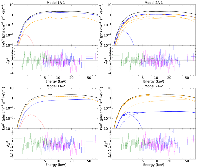
Figure 6: Model and residual plots for EXO 1846–031 with NuSTAR+NICER data. In the left panel, the red lines represent the thermal components, the blue lines represent the power-law components, and orange lines represent the reflection components. In the right panel, the blue lines represent the Comptonized thermal spectra and the orange lines represent the Comptonized reflection spectra. For the lines with same color, solid lines represent the complete spectra, dotted lines represent the components scattered by the corona, and dashed lines represent the components transmitted by the corona.

IV Discussion

IV.1 Impact of reflection Comptonization

In our study, we use NICER and NuSTAR data of EXO 1846–031 to investigate the impact of Comptonization of the reflection component on the measurements of the spectral parameters. In Model 2, the Comptonized reflection spectrum is produced by simplcutx*relxillionCp_nk, while there is no Comptonized reflection spectrum in Model 1.

We do not see significant differences in the parameter estimation between Model 1 and Model 2 (Table 3 and Table 4). The key-parameters, such as $a_{*}$ and $i$, are quite similar at $3\sigma$ confidence level (see Fig. 7), indicating that the parameter measurements are not affected. In addition, the reduced $\chi^{2}$ and AICc are also very close to each other. Possibly, stronger differences in those key parameters would manifest in the case of larger $f_{\rm SC}$ (viz: $f_{\rm SC}>$ 0.2). Other studies also suggest that the inclusion of reflection Comptonization does not significantly influence reflection spectrum fitting; see, e.g., Refs. Dong et al. (2022); Liu et al. (2023, 2022).

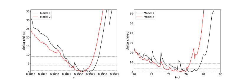
Figure 7: The 1-D $\chi^{2}$ contours for black hole spin and inclination angle for Model 1A and Model 2A with NuSTAR data. The horizontal dash line represents the $1\sigma$, $2\sigma$, $3\sigma$ confidence levels for a single parameter.

The scattered fraction $f_{\rm SC}$ in simplcutx depends on the coronal geometry and optical depth. Liu et al. (2023) found that the scattering fraction decreases during the hard-to-soft transition of GX 339–4 in the outburst in 2021 observed by Insight-HXMT. Wang et al. (2022) studied the reverberation lag of EXO 1846–031 to infer the disk-corona geometry and concluded that the corona may be the base of the jet and that the vertical extension of the jet changes during the hard-to-soft transition. These studies support the idea of an evolving corona across state transition in X-ray binaries, one measure of which is the scattering fraction. In this case, although the model formalism with simplcutx does not improve the fit statistically, in such a case looking for changes of $f_{\rm SC}$ with state may provide its own useful consistency check.

IV.2 Impact of soft X-ray data

From the comparison of the results from the analyses of the NuSTAR and NuSTAR+NICER data, we see the impact of the soft X-ray band in the analysis of the data. The disk component peaks around 2.0-3.0 keV (see Fig. 6), but NuSTAR lacks coverage below 3.0 keV. Consequently, the fit of the disk component with NuSTAR data may not be as accurate as the fit with NuSTAR+NICER data. In terms of parameters estimation, while some parameters differ slightly (e.g. $N_{\rm H}$, $T_{\rm in}$), key parameters such as spin and inclination angle still do not change significantly. It is tentatively suggested that the inclusion of soft X-ray data does not significantly impact the parameter estimations of the best-fit model. However, by including NICER soft X-ray data, we identify an additional $\chi^{2}$ minimum, not as deep, which exhibits a more reasonable flux of the disk component despite having a slightly higher AICc; see the columns of Models 1A-2 and 2A-2 in Table 4.

The mass and distance of EXO 1846-031 have not been dynamically measured yet. Studies of spectral analysis suggest mass measurements ranging from 3.24 to 7.1-12.43 $M_{\odot}$ (Strohmayer and Nicer Observatory Science Working Group, 2020; Nath et al., 2024), and distance measurements ranging from 2.4 to 7 kpc (Parmar et al., 1993; Williams et al., 2022). Considering a distance of 7 kpc and a mass in the range 5 to 12 $M_{\odot}$, the Eddington ratio $L/L_{\rm Edd}$ is 21.6%–51.7% for Model 1A-1, 18%–43% for Model 2A-1, 7.7%–13% for Model 1A-2, and 7.8%–13% for Model 2A-2. Furthermore, the unabsorbed disk component is much fainter in Models 1A-2 and 2A-2 (refer to the “disk/total” raw in Table 4). This indicates that for certain values of mass and distance, the luminosity of Models 1A-1 and 2A-1 is too high, while the results of Models 1A-2 and 2A-2 are more reasonable.

From the norm of diskbb, we can derive an approximate inner radius (Mitsuda et al., 1984):

$${\rm Norm}=(r_{\rm in}/D_{10})^{2}\;\cos\theta,$$ (5)

where $D_{10}$ is the distance in the units of 10 kpc and $r_{\rm in}$ is the derived inner radius from the observed data. After factoring in some correction factors (Kubota et al., 1998)

$$R_{\rm in}=\sqrt{\frac{3}{7}}\cdot\left(\frac{6}{7}\right)^{3}\cdot\kappa^{2}\cdot r_{\rm in},$$ (6)

where $\kappa\sim 1.7$ is the ratio of color temperature to effective temperature (Shimura and Takahara, 1995), then we can obtain $R_{\rm in}$ which is the true inner radius. For a Kerr black hole, $R_{\rm ISCO}$ (radius of the innermost stable circular orbit) can be derived from the spin (Bardeen et al., 1972). Since we apply X-ray reflection spectroscopy to measure the spin, we should identify the $R_{\rm in}$ with $R_{\rm ISCO}$ (Bambi et al., 2021). Although the estimates of $R_{\rm in}$ and $R_{\rm ISCO}$ from observed data have significant uncertainty due to the lack of accurate measurements of mass and distance, $R_{\rm in}$ should not be much larger than $R_{\rm ISCO}$ given the reflection-fitting results. $R_{\rm in}$ inferred from the results of Model 1A-1 and 2A-1 is about 9.7-70 $R_{\rm ISCO}$ (with the same uncertainty of mass and distance in estimation of Eddington ratio), while from the results of Model 1A-2 and 2A-2 is about 1.0-2.7 $R_{\rm ISCO}$. Therefore, the best fits of Model 1A-2 and 2A-2 are somewhat favored.

IV.3 Impact of emissivity profile

In the models with free $q_{\rm out}$, we get a flat emissivity profile at large radii with $q_{\rm out}\approx 0$. To validate these results, models with fixed $q_{\rm out}$ set to 3 were also examined, but they yielded significantly poorer best-fit results ($\Delta\rm AICc\sim 60$, as shown in Table 3 and Table 4) compared to the best-fit with free $q_{\rm out}$ in both NuSTAR data and NuSTAR+NICER data, with several parameters displaying notable differences. Additionally, models incorporating an additional xillverCp component were tested to explore the possibility of obtaining a larger value for $q_{\rm out}$. However, the norm of xillverCp is consistent with zero. Furthermore, in the results of the NuSTAR+NICER data in Model 1A-2 and Model 2A-2, the index $q_{\rm out}\gtrsim 1$, which alleviates concerns about a runway emissivity for $q_{\rm out}\sim 0$ (as illustrated in Fig. 4), so we only show the results of emissivity profile “A” in Table 4. Other studies also reported instances of $q_{\rm out}\approx 0$ in GS 1354–645 (Xu et al., 2018) and GRS 1915+105 (Zhang et al., 2019).

V Conclusions

We investigated the impact of the Comptonization of the reflection spectrum in the case of EXO 1846–031. We have drawn the following conclusions:

1. Considering reflection Comptonization by using simplcutx does not yield a significantly different best fit and it does not affect the values of key parameters such as black hole spin and inclination angle. In the case of coronal properties evolving during state transitions, the variation in $f_{\rm SC}$ potentially providing a useful consistency check.

2. The inclusion of soft X-ray data does not significantly affect the estimations of key parameters, but gives a new fit with more reasonable luminosity, inner radius of disk and emissivity profile. The fit of NuSTAR+NICER data with a weak disk component and non-zero $q_{\rm out}$ is the most reasonable in this case.

Acknowledgments – This work was supported by the Natural Science Foundation of Shanghai, Grant No. 22ZR1403400, and the National Natural Science Foundation of China (NSFC), Grant No. 12250610185, 11973019, and 12261131497.

References

- Bambi et al. (2021) C. Bambi, L. W. Brenneman, T. Dauser, J. A. García, V. Grinberg, A. Ingram, J. Jiang, H. Liu, A. M. Lohfink, A. Marinucci, G. Mastroserio, R. Middei, S. Nampalliwar, A. Niedźwiecki, J. F. Steiner, A. Tripathi, and A. A. Zdziarski, Space Sci. Rev. 217, 65 (2021).
- Fabian et al. (1995) A. C. Fabian, K. Nandra, C. S. Reynolds, W. N. Brandt, C. Otani, Y. Tanaka, H. Inoue, and K. Iwasawa, Mon. Not. R. Astron. Soc. 277, L11 (1995), arXiv:astro-ph/9507061 [astro-ph] .
- Zoghbi et al. (2010) A. Zoghbi, A. C. Fabian, P. Uttley, G. Miniutti, L. C. Gallo, C. S. Reynolds, J. M. Miller, and G. Ponti, Mon. Not. R. Astron. Soc. 401, 2419 (2010), arXiv:0910.0367 [astro-ph.HE] .
- Risaliti et al. (2013) G. Risaliti, F. A. Harrison, K. K. Madsen, D. J. Walton, S. E. Boggs, F. E. Christensen, W. W. Craig, B. W. Grefenstette, C. J. Hailey, E. Nardini, D. Stern, and W. W. Zhang, Nature (London) 494, 449 (2013), arXiv:1302.7002 [astro-ph.HE] .
- Novikov and Thorne (1973) I. D. Novikov and K. S. Thorne, in Black Holes (Les Astres Occlus) (1973) pp. 343–450.
- Ross and Fabian (2005) R. R. Ross and A. C. Fabian, Mon. Not. R. Astron. Soc. 358, 211 (2005), arXiv:astro-ph/0501116 [astro-ph] .
- García and Kallman (2010) J. García and T. R. Kallman, Astrophys. J. 718, 695 (2010), arXiv:1006.0485 [astro-ph.HE] .
- Steiner et al. (2016) J. F. Steiner, R. A. Remillard, J. A. García, and J. E. McClintock, Astrophys. J. 829, L22 (2016), arXiv:1609.04592 [astro-ph.HE] .
- Steiner et al. (2017) J. F. Steiner, J. A. García, W. Eikmann, J. E. McClintock, L. W. Brenneman, T. Dauser, and A. C. Fabian, Astrophys. J. 836, 119 (2017), arXiv:1701.03777 [astro-ph.HE] .
- Wilkins and Gallo (2015) D. R. Wilkins and L. C. Gallo, Mon. Not. R. Astron. Soc. 448, 703 (2015), arXiv:1412.0015 [astro-ph.HE] .
- Parmar and White (1985) A. N. Parmar and N. E. White, IAU Circ. 4051, 1 (1985).
- Negoro et al. (2019) H. Negoro, M. Nakajima, S. Sugita, R. Sasaki, W. I. T. Mihara, W. Maruyama, M. Aoki, K. Kobayashi, T. Tamagawa, M. Matsuoka, T. Sakamoto, M. Serino, H. Nishida, A. Yoshida, Y. Tsuboi, H. Kawai, T. Sato, M. Shidatsu, N. Kawai, M. Sugizaki, M. Oeda, K. Shiraishi, S. Nakahira, Y. Sugawara, S. Ueno, H. Tomida, M. Ishikawa, N. Isobe, R. Shimomukai, M. Tominaga, Y. Ueda, A. Tanimoto, S. Yamada, S. Ogawa, K. Setoguchi, T. Yoshitake, H. Tsunemi, T. Yoneyama, K. Asakura, S. Ide, M. Yamauchi, S. Iwahori, Y. Kurihara, K. Kurogi, K. Miike, T. Kawamuro, K. Yamaoka, and Y. Kawakubo, The Astronomer’s Telegram 12968, 1 (2019).
- Mereminskiy et al. (2019) I. A. Mereminskiy, R. A. Krivonos, P. S. Medvedev, and S. A. Grebenev, The Astronomer’s Telegram 12969, 1 (2019).
- Bult et al. (2019) P. M. Bult, K. C. Gendreau, Z. Arzoumanian, T. E. Strohmayer, P. S. Ray, S. Guillot, W. Iwakiri, J. Homan, D. Altamirano, G. K. Jaisawal, and J. M. Miller, The Astronomer’s Telegram 12976, 1 (2019).
- Miller et al. (2019) J. M. Miller, A. Zoghbi, P. Gandhi, and J. Paice, The Astronomer’s Telegram 13012, 1 (2019).
- Yang et al. (2019a) Y.-J. Yang, R. Soria, D. Russell, G. Xiao, J. Qu, and S.-N. Zhang, The Astronomer’s Telegram 13036, 1 (2019a).
- Yang et al. (2019b) Y.-J. Yang, G. Xiao, R. Soria, D. Russell, J. Qu, and S.-N. Zhang, The Astronomer’s Telegram 13037, 1 (2019b).
- Draghis et al. (2020) P. A. Draghis, J. M. Miller, E. M. Cackett, E. S. Kammoun, M. T. Reynolds, J. A. Tomsick, and A. Zoghbi, Astrophys. J. 900, 78 (2020), arXiv:2007.04324 [astro-ph.HE] .
- Abdikamalov et al. (2021) A. B. Abdikamalov, D. Ayzenberg, C. Bambi, H. Liu, and Y. Zhang, Phys. Rev. D 103, 103023 (2021), arXiv:2101.10100 [astro-ph.HE] .
- Tripathi et al. (2021a) A. Tripathi, A. B. Abdikamalov, D. Ayzenberg, C. Bambi, and H. Liu, Astrophys. J. 913, 129 (2021a), arXiv:2102.04695 [astro-ph.HE] .
- Tripathi et al. (2021b) A. Tripathi, B. Zhou, A. B. Abdikamalov, D. Ayzenberg, and C. Bambi, JCAP 2021, 002 (2021b), arXiv:2103.07593 [astro-ph.HE] .
- Yu et al. (2021) Z. Yu, Q. Jiang, A. B. Abdikamalov, D. Ayzenberg, C. Bambi, H. Liu, S. Nampalliwar, and A. Tripathi, Phys. Rev. D 104, 084035 (2021), arXiv:2106.11658 [astro-ph.HE] .
- Gu et al. (2022) J. Gu, S. Riaz, A. B. Abdikamalov, D. Ayzenberg, and C. Bambi, European Physical Journal C 82, 708 (2022), arXiv:2206.14733 [gr-qc] .
- Tao et al. (2023) J. Tao, S. Riaz, B. Zhou, A. B. Abdikamalov, C. Bambi, and D. Malafarina, Phys. Rev. D 108, 083036 (2023), arXiv:2301.12164 [gr-qc] .
- Liu et al. (2021) H.-X. Liu, Y. Huang, G.-C. Xiao, Q.-C. Bu, J.-L. Qu, S. Zhang, S.-N. Zhang, S.-M. Jia, F.-J. Lu, X. Ma, L. Tao, W. Zhang, L. Chen, L.-M. Song, T.-P. Li, Y.-P. Xu, X.-L. Cao, Y. Chen, C.-Z. Liu, C. Cai, Z. Chang, G. Chen, T.-X. Chen, Y.-B. Chen, Y.-P. Chen, W. Cui, W.-W. Cui, J.-K. Deng, Y.-W. Dong, Y.-Y. Du, M.-X. Fu, G.-H. Gao, H. Gao, M. Gao, M.-Y. Ge, Y.-D. Gu, J. Guan, C.-C. Guo, D.-W. Han, J. Huo, L.-H. Jiang, W.-C. Jiang, J. Jin, Y.-J. Jin, L.-D. Kong, B. Li, C.-K. Li, G. Li, M.-S. Li, W. Li, X. Li, X.-B. Li, X.-F. Li, Y.-G. Li, Z.-W. Li, X.-H. Liang, J.-Y. Liao, B.-S. Liu, G.-Q. Liu, H.-W. Liu, X.-J. Liu, Y.-N. Liu, B. Lu, X.-F. Lu, Q. Luo, T. Luo, B. Meng, Y. Nang, J.-Y. Nie, G. Ou, N. Sai, R.-C. Shang, X.-Y. Song, L. Sun, Y. Tan, Y.-L. Tuo, C. Wang, G.-F. Wang, J. Wang, L.-J. Wang, W.-S. Wang, Y.-S. Wang, X.-Y. Wen, B.-Y. Wu, B.-B. Wu, M. Wu, S. Xiao, S.-L. Xiong, H. Xu, J.-W. Yang, S. Yang, Y.-J. Yang, Y.-J. Yang, Q.-B. Yi, Q.-Q. Yin, Y. You, A.-M. Zhang, C.-M. Zhang, F. Zhang, H.-M. Zhang, J. Zhang, T. Zhang, W.-C. Zhang, W.-Z. Zhang, Y. Zhang, Y.-F. Zhang, Y.-J. Zhang, Y.-H. Zhang, Y. Zhang, Z. Zhang, Z. Zhang, Z.-L. Zhang, H.-S. Zhao, X.-F. Zhao, S.-J. Zheng, Y.-G. Zheng, D.-K. Zhou, J.-F. Zhou, Y.-X. Zhu, R.-L. Zhuang, and Y. Zhu, Research in Astronomy and Astrophysics 21, 070 (2021), arXiv:2009.10956 [astro-ph.HE] .
- Wang et al. (2021) Y. Wang, L. Ji, J. A. García, T. Dauser, M. Méndez, J. Mao, L. Tao, D. Altamirano, P. Maggi, S. N. Zhang, M. Y. Ge, L. Zhang, J. L. Qu, S. Zhang, X. Ma, F. J. Lu, T. P. Li, Y. Huang, S. J. Zheng, Z. Chang, Y. L. Tuo, L. M. Song, Y. P. Xu, Y. Chen, C. Z. Liu, Q. C. Bu, C. Cai, X. L. Cao, L. Chen, T. X. Chen, Y. P. Chen, W. W. Cui, Y. Y. Du, G. H. Gao, Y. D. Gu, J. Guan, C. C. Guo, D. W. Han, J. Huo, S. M. Jia, W. C. Jiang, J. Jin, L. D. Kong, B. Li, C. K. Li, G. Li, W. Li, X. Li, X. B. Li, X. F. Li, Z. W. Li, X. H. Liang, J. Y. Liao, H. W. Liu, X. J. Liu, X. F. Lu, Q. Luo, T. Luo, B. Meng, Y. Nang, J. Y. Nie, G. Ou, N. Sai, R. C. Shang, X. Y. Song, L. Sun, Y. Tan, W. S. Wang, Y. D. Wang, Y. S. Wang, X. Y. Wen, B. B. Wu, B. Y. Wu, M. Wu, G. C. Xiao, S. Xiao, S. L. Xiong, S. Yang, Y. J. Yang, Q. B. Yi, Q. Q. Yin, Y. You, F. Zhang, H. M. Zhang, J. Zhang, W. C. Zhang, W. Zhang, Y. F. Zhang, H. S. Zhao, X. F. Zhao, and D. K. Zhou, Astrophys. J. 906, 11 (2021), arXiv:2010.14662 [astro-ph.HE] .
- Ren et al. (2022) X. Q. Ren, Y. Wang, S. N. Zhang, R. Soria, L. Tao, L. Ji, Y. J. Yang, J. L. Qu, S. Zhang, L. M. Song, M. Y. Ge, Y. Huang, X. B. Li, J. Y. Liao, H. X. Liu, R. C. Ma, Y. L. Tuo, P. J. Wang, W. Zhang, and D. K. Zhou, Astrophys. J. 932, 66 (2022), arXiv:2205.04635 [astro-ph.HE] .
- Madsen et al. (2022) K. K. Madsen, K. Forster, B. Grefenstette, F. A. Harrison, and H. Miyasaka, Journal of Astronomical Telescopes, Instruments, and Systems 8, 034003 (2022), arXiv:2110.11522 [astro-ph.IM] .
- Kaastra and Bleeker (2016) J. S. Kaastra and J. A. M. Bleeker, Astron. Astrophys. 587, A151 (2016), arXiv:1601.05309 [astro-ph.IM] .
- Remillard et al. (2022) R. A. Remillard, M. Loewenstein, J. F. Steiner, G. Y. Prigozhin, B. LaMarr, T. Enoto, K. C. Gendreau, Z. Arzoumanian, C. Markwardt, A. Basak, A. L. Stevens, P. S. Ray, D. Altamirano, and D. J. K. Buisson, Astron. J. 163, 130 (2022), arXiv:2105.09901 [astro-ph.IM] .
- Arnaud (1996) K. A. Arnaud, in Astronomical Data Analysis Software and Systems V, Astronomical Society of the Pacific Conference Series, Vol. 101, edited by G. H. Jacoby and J. Barnes (1996) p. 17.
- Tao et al. (2019) L. Tao, J. A. Tomsick, J. Qu, S. Zhang, S. Zhang, and Q. Bu, Astrophys. J. 887, 184 (2019), arXiv:1910.11979 [astro-ph.HE] .
- Nath et al. (2024) S. K. Nath, D. Debnath, K. Chatterjee, R. Bhowmick, H.-K. Chang, and S. K. Chakrabarti, Astrophys. J. 960, 5 (2024), arXiv:2307.04522 [astro-ph.HE] .
- Wilms et al. (2000) J. Wilms, A. Allen, and R. McCray, Astrophys. J. 542, 914 (2000), arXiv:astro-ph/0008425 [astro-ph] .
- Pringle (1981) J. E. Pringle, Annu. Rev. Astron. Astrophys. 19, 137 (1981).
- Mitsuda et al. (1984) K. Mitsuda, H. Inoue, K. Koyama, K. Makishima, M. Matsuoka, Y. Ogawara, N. Shibazaki, K. Suzuki, Y. Tanaka, and T. Hirano, Publ. Astron. Soc. Japan 36, 741 (1984).
- Zdziarski et al. (1996) A. A. Zdziarski, W. N. Johnson, and P. Magdziarz, Monthly Notices of the Royal Astronomical Society 283, 193 (1996).
- Życki et al. (1999) P. T. Życki, C. Done, and D. A. Smith, Mon. Not. R. Astron. Soc. 309, 561 (1999), arXiv:astro-ph/9904304 [astro-ph] .
- Smith et al. (2016) R. K. Smith, L. A. Valencic, and L. Corrales, Astrophys. J. 818, 143 (2016), arXiv:1602.07766 [astro-ph.HE] .
- Barillier et al. (2023) E. Barillier, V. Grinberg, D. Horn, M. A. Nowak, R. A. Remillard, J. F. Steiner, D. J. Walton, and J. Wilms, Astrophys. J. 944, 165 (2023), arXiv:2301.09226 [astro-ph.HE] .
- Steiner et al. (2010) J. F. Steiner, J. E. McClintock, R. A. Remillard, L. Gou, S. Yamada, and R. Narayan, Astrophys. J. 718, L117 (2010), arXiv:1006.5729 [astro-ph.HE] .
- Burnham (1998) K. P. Burnham, A practical information-theoretic approach (1998).
- Akaike (1974) H. Akaike, IEEE Transactions on Automatic Control 19, 716 (1974).
- Dong et al. (2022) Y. Dong, Z. Liu, Y. Tuo, J. F. Steiner, M. Ge, J. A. García, and X. Cao, Mon. Not. R. Astron. Soc. 514, 1422 (2022), arXiv:2205.12058 [astro-ph.HE] .
- Liu et al. (2023) H. Liu, C. Bambi, J. Jiang, J. A. García, L. Ji, L. Kong, X. Ren, S. Zhang, and S. Zhang, Astrophys. J. 950, 5 (2023), arXiv:2211.09543 [astro-ph.HE] .
- Liu et al. (2022) Q. Liu, H. Liu, C. Bambi, and L. Ji, Mon. Not. R. Astron. Soc. 512, 2082 (2022), arXiv:2111.00719 [astro-ph.HE] .
- Wang et al. (2022) J. Wang, E. Kara, M. Lucchini, A. Ingram, M. van der Klis, G. Mastroserio, J. A. García, T. Dauser, R. Connors, A. C. Fabian, J. F. Steiner, R. A. Remillard, E. M. Cackett, P. Uttley, and D. Altamirano, Astrophys. J. 930, 18 (2022), arXiv:2205.00928 [astro-ph.HE] .
- Strohmayer and Nicer Observatory Science Working Group (2020) T. E. Strohmayer and Nicer Observatory Science Working Group, in American Astronomical Society Meeting Abstracts #235, American Astronomical Society Meeting Abstracts, Vol. 235 (2020) p. 159.02.
- Parmar et al. (1993) A. N. Parmar, L. Angelini, P. Roche, and N. E. White, Astron. Astrophys. 279, 179 (1993).
- Williams et al. (2022) D. R. A. Williams, S. E. Motta, R. Fender, J. C. A. Miller-Jones, J. Neilsen, J. R. Allison, J. Bright, I. Heywood, P. F. L. Jacob, L. Rhodes, E. Tremou, P. A. Woudt, J. v. d. Eijnden, F. Carotenuto, D. A. Green, D. Titterington, A. J. van der Horst, and P. Saikia, Mon. Not. R. Astron. Soc. 517, 2801 (2022), arXiv:2209.10228 [astro-ph.HE] .
- Kubota et al. (1998) A. Kubota, Y. Tanaka, K. Makishima, Y. Ueda, T. Dotani, H. Inoue, and K. Yamaoka, Publ. Astron. Soc. Japan 50, 667 (1998).
- Shimura and Takahara (1995) T. Shimura and F. Takahara, Astrophys. J. 445, 780 (1995).
- Bardeen et al. (1972) J. M. Bardeen, W. H. Press, and S. A. Teukolsky, Astrophys. J. 178, 347 (1972).
- Xu et al. (2018) Y. Xu, S. Nampalliwar, A. B. Abdikamalov, D. Ayzenberg, C. Bambi, T. Dauser, J. A. García, and J. Jiang, Astrophys. J. 865, 134 (2018), arXiv:1807.10243 [gr-qc] .
- Zhang et al. (2019) Y. Zhang, A. B. Abdikamalov, D. Ayzenberg, C. Bambi, and S. Nampalliwar, Astrophys. J. 884, 147 (2019), arXiv:1907.03084 [gr-qc] .