PACP: Priority-Aware Collaborative Perception for Connected and Autonomous Vehicles

Abstract

Surrounding perceptions are quintessential for safe driving for connected and autonomous vehicles (CAVs), where the Bird’s Eye View has been employed to accurately capture spatial relationships among vehicles. However, severe inherent limitations of BEV, like blind spots, have been identified. Collaborative perception has emerged as an effective solution to overcoming these limitations through data fusion from multiple views of surrounding vehicles. While most existing collaborative perception strategies adopt a fully connected graph predicated on fairness in transmissions, they often neglect the varying importance of individual vehicles due to channel variations and perception redundancy. To address these challenges, we propose a novel Priority-Aware Collaborative Perception (PACP) framework to employ a BEV-match mechanism to determine the priority levels based on the correlation between nearby CAVs and the ego vehicle for perception. By leveraging submodular optimization, we find near-optimal transmission rates, link connectivity, and compression metrics. Moreover, we deploy a deep learning-based adaptive autoencoder to modulate the image reconstruction quality under dynamic channel conditions. Finally, we conduct extensive studies and demonstrate that our scheme significantly outperforms the state-of-the-art schemes by 8.27% and 13.60%, respectively, in terms of utility and precision of the Intersection over Union.

1 Introduction

1.1 Background

Recent advances in positioning and perception have emerged as pivotal components in numerous cutting-edge applications, most notably in autonomous driving[1, 2, 3, 4]. These systems heavily rely on precise positioning and acute perception capabilities to safely and adeptly navigate complex road environments. Many solutions exist for positioning and perception in CAVs, including inertial navigation systems, high-precision GPS, cameras, and LiDAR[5]. However, any isolated use of them may not be enough to achieve the desired level of perception quality for safe driving. In contrast, the Bird’s Eye View (BEV) stands out as a more holistic approach. By integrating data from multiple sensors and cameras placed around a vehicle, BEV offers a comprehensive, potentially 360-degree view of a vehicle’s surroundings, offering a more contextually rich understanding of its environment[6]. However, most BEV-aided perception designs have predominantly concentrated on single-vehicle systems. Such an approach may not be enough in high-density traffic scenarios, where unobservable blind spots caused by road obstacles or other vehicles remain a significant design challenge. Therefore, collaborative perception has become a promising candidate for autonomous driving. To mitigate the limitations of the single-vehicle systems, we can leverage multiple surrounding CAVs to obtain a more accurate BEV prediction via multi-sensor fusion[7].

To further reduce the risks of blind spots in BEV prediction, collaborative perception is adapted to enable multiple vehicles to share more complementary surrounding information with each other through vehicle-to-vehicle (V2V) communications[8]. This framework intrinsically surmounts several inherent constraints tied to single-agent perception, including occlusion and long-range detection limitation. Similar designs have been observed in a variety of practical scenarios, including communication-assisted autonomous driving within the realm of vehicle-to-everything[9], multiple aerial vehicles for accuracy perception[10], and multiple underwater vehicles deployed in search and rescue operations[11].

In this emerging field of autonomous driving, the current predominant challenge is how to make a trade-off between perception accuracy and communication resource allocation. Given the voluminous perception outputs (such as point clouds and consecutive RGB image sequences), the data transmission for CAVs demands substantial communication bandwidth. Such requirements often run into capacity bottleneck. As per the KITTI dataset[12], a single frame from 3-D Velodyne laser scanners encompasses approximately 100,000 data points, where the smallest recorded scenario has 114 frames, aggregating to an excess of 10 million data points. Thus, broadcasting such extensive data via V2V communications amongst a vast array of CAVs becomes a daunting task. Therefore, it is untenable to solely emphasize the perception efficiency enhancement without considering the overhead on V2V communications. Thereby, some existing studies propose various communication-efficient collaboration frameworks, such as the edge-aided perception framework[13] and the transmission scheme for compressed deep feature map[14]. It is observed that all these approaches can be viewed as fairness-based schemes, i.e., each vehicle within a certain range should have a fair chance to convey its perception results to the ego vehicle. Among all transmission strategies used for collaborative perception, the fairness-based scheme is the most popular one owing to its low computational complexity.

Despite the low computational complexity, several major design challenges still exist with the state-of-the-art fairness-based schemes, entailing the adaptation of these perception approaches in real-world scenarios:

• Fairness-based schemes may lead to overlapping data transmissions from multiple vehicles, causing unnecessary duplications and bandwidth wastage.

• Fairness-based schemes cannot inherently prioritize perception results from closer vehicles, which may be more critical than those from further vehicles.

• Without differentiating the priority of data from different vehicles, fairness-based schemes may block communication channels for more crucial information.

To address the above challenges, we conceive a priority-aware perception framework with the BEV-match mechanism, which acquires the correlation between nearby CAVs and the ego CAV. Compared with the fairness-based schemes, the proposed approach pays attention to the balance between the correlation and sufficient extra information. Therefore, this method not only optimizes perception efficiency by preventing repetitive data, but also enhances the robustness of perception under the limited bandwidth of V2V communications.

In the context of collaborative perception, a significant concern revolves efficient collaborative perception over time-invariant links. The earlier research on cooperative perception has considered lossy channels [15] and link latency[16]. However, most existing research leans heavily on the assumption of an ideal communication channel without packet loss, overlooking the effects of fluctuating network capacity[8]. Moreover, establishing fusion links among nearby CAVs is a pivotal aspect that needs attention. Existing strategies are often based on basic proximity constructs, neglecting the dynamic characteristics of the wireless channel shared among CAVs. In contrast, graph-based optimization techniques provide a more adaptive approach, accounting for real-world factors like signal strength and bandwidth availability to improve network throughput.

A significant challenge in adopting these graph-based techniques is to manage the transmission load of V2V communications for point cloud and camera data. With the vast amount of data produced by CAVs, it is crucial to compress this data. Spatial redundancy is usually addressed by converting raw high-definition data into 2D matrix form. To tackle temporal redundancy, video-based compression techniques are applied. However, traditional compression techniques, such as JPEG[17] and MPEG[18], are not always ideal for time-varying channels. This highlights the relevance of modulated autoencoders and data-driven learning-based compression methods that outperform traditional methods. These techniques excel at encoding important features while discarding less relevant ones. Moreover, the adoption of fine-tuning strategies improves the quality of reconstructed data, whereas classical techniques often face feasibility issues.

1.2 State-of-the-Art

In this subsection, we review the related literature of collaborative perception for autonomous driving with an emphasis on their perceptual algorithms, network optimization, and redundant information reduction.

V2V collaborative perception: V2V collaborative perception combines the sensed data from different CAVs through fusion networks, thereby expanding the perception range of each CAV and mitigating troubling design issues like blind spots. For instance, Chen et al. [19] proposed the early fusion scheme, which fuses raw data from different CAVs, while Wang et al. [14] employed intermediate fusion, fusing intermediate features from various CAVs, and Rawashdeh et al. [20] utilized late fusion, combining detection outputs from different CAVs to accomplish collaborative perception tasks. Although these methods show promising results under ideal conditions, in real-world environments, where the channel conditions are highly variable, directly applying the same fusion methods often results in unsatisfactory outcomes.

Network optimization: High throughput can ensure more efficient data transmissions among CAVs, thereby potentially improving the IoU of cooperative perception systems. Lyu et al.[21] proposed a fully distributed graph-based throughput optimization framework by leveraging submodular optimization. Nguyen et al.[22] designed a cooperative technique, aiming to enhance data transmission reliability and improve throughput by successively selecting relay vehicles from the rear to follow the preceding vehicles. Ma et al.[23] developed an efficient scheme for the throughput optimization problem in the context of highly dynamic user requests. However, the intricate relationship between throughput maximization and IoU has not been thoroughly investigated in the literature. This gap in the research motivates us to conduct more comprehensive studies on the role of throughput optimization in V2V cooperative perception.

Vehicular data compression: For V2V collaborative perception, participating vehicles compress their data before transmitting it to the ego vehicle to reduce transmission latency. However, existing collaborative frameworks often employ very simple compressors, such as the naive encoder consisting of only one convolutional layer used in V2VNet[14]. Such compressors cannot meet the requirement of transmission latency under $100$ ms in practical collaborative tasks[24]. Additionally, current views suggest that compressors composed of neural networks outperform the compressors based on traditional algorithms[25]. However, these studies are typically focused on general data compression tasks and lack research on adaptive compressors suitable for practical scenarios in V2V collaborative perception.

1.3 Our Contributions

TABLE I: CONTRASTING OUR CONTRIBUTION TO THE LITERATURE

	[an2024throughput]	[3]	[2]	[15]	[10]	[13]	[14]	[19]	[20]	[21]	[22]	[23]	[26]	Proposed work
BEV evaluation	✓	✓	✓	✓			✓							✓
Multi-agent selection	✓		✓		✓	✓	✓	✓		✓	✓		✓	✓
Data compression	✓		✓		✓	✓	✓	✓						✓
Lossy communications	✓		✓	✓					✓	✓	✓		✓	✓
Priority mechanism													✓	✓
Coverage optimization					✓						✓		✓	✓
Throughput optimization	✓		✓							✓	✓	✓	✓	✓

To address the weakness of prior works and tackle the aforementioned design challenges, we design our Priority-Aware Collaborative Perception (PACP) framework for CAVs and evaluate its performance on a CAV simulation platform CARLA[27] with OPV2V dataset[28]. Experimental results verify PACP’s superior performance, with notable improvements in utility value and the average precision of Intersection over Union (AP@IoU) compared with existing methods. To summarize, in this paper, we have made the following major contributions:

• This is the first paper to leverage a priority-aware collaborative perception framework involving a carefully designed BEV-match mechanism for autonomous driving, which strikes a balance between the communication overhead and perception accuracy.

• To enhance transmission quality, we employ a two-stage optimization framework based on submodular theory to jointly optimize transmission rates, link connectivity, and compression ratio, addressing challenges of data-intensive transmissions under constrained time-varying channel capacity.

• We design and implement a deep learning-based adaptive autoencoder integrated into PACP, assisted by fine-tuning mechanisms at roadside units (RSUs). The experimental evaluation reveals that this approach surpasses the state-of-the-art methods, especially in utility value and AP@IoU.

Our new contributions are better illustrated in Table I.

2 Fairness or Priority?

In this section, we show some practical difficulties with fairness-based collaborative perception for CAVs and also briefly demonstrate the superiority of adopting a priority-aware perception framework.

2.1 Background of Two Schemes

(1) Fairness-based perception scheme: For perception data from different sources, achieving fairness is a popular design goal[29], which ensures that equal resources for different resources to transmit perception data in V2V networks. The Jain’s fairness index $J$ is the most popular metric to characterize the fairness[26]:

$$J=\frac{(\sum_{i=1}^{n}x_{i})^{2}}{n\cdot\sum_{i=1}^{n}x_{i}^{2}},$$ (1)

where $n$ is the total number of nodes and $x_{i}$ is the resource allocated to the $i$-th node. According to Cauchy-Schwartz inequality, its value ranges from $(0,1]$, which is equal to 1 if and only if all $x_{i}$ are equal, i.e., 1 indicates perfect fairness. Based on the type of resources, two popular fairness schemes are the subchannel- and throughput-fairness schemes, respectively. Specifically, the subchannel-fairness scheme means each CAV can be allocated the same amount of spectrum resources while the throughput-fairness scheme requires each CAV to have the same transmission rate.

(2) Priority-aware perception scheme: Traditional fairness-based schemes treat all CAVs equally, potentially enhancing the quality of less important information while diminishing the quality of crucial data, consequently reducing the efficiency of the system. Therefore, it is crucial to determine the priority of the sensed data from the nearby CAVs. Existing works have investigated several popular priority factors as priority, such as link latency[30] and routing situation[31]. However, previous studies failed to investigate the negative effects of a “poisonous” CAV, which transmits its perception result to ego CAV but aggravates the performance of collaborative perception because of poor channel condition and specific location. Therefore, the ego vehicle gives higher priority to the vehicles with more important data and better BEV match (refer to details in Sec. 4.2). In so doing, the ego CAV assigns a lower priority to those poisonous CAVs, mitigating the adverse impact on AP@IoU.

2.2 Comparison Between Fairness and Priority

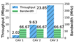
(a) Subchannel-fairness scheme

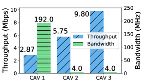
(b) Throughput-fairness scheme

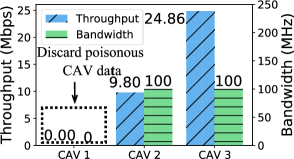
(c) Priority-aware perception scheme

Figure 1: The bandwidth and throughput allocation by different schemes within V2V network.

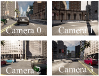
(a) Camera perception by ego CAV

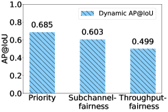
(b) AP@IoU vs. Different schemes

Figure 2: Camera data and different types of AP@IoU.

To better understand the limitations of fairness-based schemes, we use two typical fairness-based schemes to showcase their resource allocation and BEV prediction in comparison to the priority-aware scheme. Fig. 1 shows the bandwidth and throughput allocation of three schemes in a V2V network. In our scenario, the ego CAV exploits three schemes to combine three nearby CAVs’ camera perception results for BEV prediction, respectively. The whole bandwidth is 200 MHz. Due to the worst channel condition, it is noted that CAV 1 has the lowest priority, thereby its data is discarded by the priority-aware scheme. Fig. 1(b) shows that the compensation of throughput-fairness scheme for weaker channels by allocating more resources results in a decrease in BEV prediction accuracy. Specifically, if a CAV’s channel quality is extremely poor (e.g., CAV 1), the allocated discrete bandwidth might still be insufficient to ensure equalized throughput. In Fig. 2(a), we show the camera perception results from the ego CAV. In Fig. 2(b), it can be observed that the impact of different communication conditions on the dynamic AP@IoU (mobile objective detection) is significant. Additionally, the superiority of the priority-aware scheme becomes evident in Fig. 2(b), where the dynamic AP@IoU rises to 0.685. Therefore, the priority-aware scheme surpasses the fairness-based methods by discerningly choosing which CAVs to collaborate with, leading to improved BEV predictions.

3 System Model

In this section, we present a V2X-aided collaborative perception system with CAVs, including the system’s structure, channel modeling, and the constraints of computational capacity and energy.

3.1 System Overview

We consider a V2X-aided collaborative perception system with multiple CAVs and RSUs, which is shown in Fig. 3. In our scenario, CAVs can be divided into two types. The first type is the nearby CAVs (indexes 1-3), which monitor the surrounding traffic with cameras and share their perception results with other CAVs. The second type is the ego CAV (index $0$), which fuses the camera data from the nearby CAVs with its own perception results. As shown in Fig. 3, the ego CAV $0$ is covered with the parked car that the ego CAV’s own camera cannot observe the incoming pedestrian from the blind spot. Through the collaborative perception scheme, the ego CAV merges compressed data from CAVs 2 and 3, i.e., $s_{20}=s_{30}=1$, which catch the existence of the pedestrian. However, it is unnecessary to connect all CAVs together since the bandwidth and subchannel resources are limited. Therefore, the ego CAV can determine the importance of each nearby CAV by the priority-aware mechanism, depending on CAVs’ positions and channel states. For example, the ego CAV is disconnected from CAV 1, because it fails to provide enough environmental perception information, i.e., $s_{10}=0$. For the sake of maximizing AP@IoU, the ego CAV obtains the near-optimal solution in terms of the transmission rate $d_{ij}$ and the compression ratio $r_{ij}$ at each time slot. Additionally, we deploy several RSUs to achieve a fine-tuning compression strategy, which is detailed in Sec. 5.4.

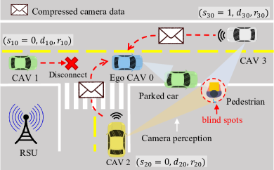
Figure 3: Overview of V2X-aided collaborative perception system.

3.2 Channel Modeling and System Constraints

Consider the V2V network architecture $\mathbf{G}=(\mathbf{V},\mathbf{E})$, where $\mathbf{V}=({v_{1},v_{2},...,v_{N}})$ denotes CAVs and $\mathbf{E}$ is the set of links between them. As per 3GPP specifications for 5G[32], V2V networks adopt Cellular Vehicle-to-Everything (C-V2X) with Orthogonal Frequency Division Multiplexing (OFDM). The total bandwidth $W$ is split into $K$ orthogonal sub-channels. Each sub-channel capacity is $C_{ij}=\frac{W}{K}\log_{2}\left(1+\frac{P_{t}h_{ij}}{N_{0}\frac{W}{K}}\right)$, where $P_{t}$ represents the transmit power, $h_{ij}$ denotes the channel gain from the $i$th transmitter to the $j$th receiver, and $N_{0}$ is the noise power spectral density.

Additionally, let $s_{ij}=1$ indicate the presence of the directional link from CAV $i$ to ego CAV $j$. Such a link is denoted as $(i,j)\in\mathcal{S}$. The set $\mathcal{S}$ represents the collection of all established links in the network. When $s_{ij}=1$, CAV $v_{i}$ is capable of sharing data with the ego CAV $v_{j}$. Conversely, if $s_{ij}=0$, it implies the disconnected mode of the link $(i,j)$. However, the number of directed links potentially increase at a rate of $N^{2}$ with the number of CAVs, possibly exhausting the limited communication spectrum resources. Therefore, the upper bound of the number of connections is given by:

$$\sum_{i=1,i\neq j}^{N}{\sum_{j=1}^{N}{s_{ij}}}\leq K.$$ (2)

Let $\mathcal{D}=\left\{d_{ij}\right\}_{N\times N}$ be the matrix consisting of transmission rates, where each element is non-negative, for $\forall(i,j)\in\mathbf{E}$. Each element $d_{ij}$ represents the data rate from vehicle $v_{i}$ to vehicle $v_{j}$ and is subsequently processed by $v_{j}$. It is noteworthy that $d_{ij}$ satisfies:

$${r}_{ij}d_{ij}\leq\min(C_{ij},A_{i}),$$ (3)

Here, ${r}_{ij}\in(0,1]$ denotes the adaptive compression ratio, obtained by the compression algorithm outlined in Sec. 5.4. $A_{i}$ signifies the amount of local perception data at $v_{i}$ per second, i.e., perception data generation rate at the location of $v_{i}$. This constraint implies that the value of $d_{ij}$ must be limited either by the achievable data rate or by the rate of perception of the local data present at vehicle $v_{i}$. Furthermore, it is observed that an inadequate compression ratio results in a diminution in the accuracy of perception data, while an excessively high compression ratio results in suboptimal throughput maximization. Consequently, the constraint for the compression ratio is defined as follows:

$$\mathbf{1}^{\top}{r}_{j,\min}\preceq\mathcal{R}_{j}\preceq\mathbf{1}^{\top}{r}_{j,\max},$$ (4)

where $\mathcal{R}_{j}=\left[\mathrm{{r}}_{{1j}},\mathrm{{r}}_{2{j}},...,\mathrm{{r}}_{{Nj}}\right]^{\top}$, ${\mathcal{R}}$ $=\left[\mathcal{R}_{1},\mathcal{R}_{2},...,\mathcal{R}_{{N}}\right]$. Given the surrounding data obtained through collaborative perception, perception data from closer vehicles are more important for perceptional detection, which has a higher level of accuracy. Therefore, we assume that the adaptive compression ratio for the link $(i,j)$ yields:

$${r}_{ij}e^{L_{ij}}\geqslant\eta,$$ (5)

where $L_{ij}$ denotes the normalized distance between $v_{i}$ and $v_{j}$, and $\eta\in(0,1]$. It is noted that we use an exponential relationship in terms of normalized distance, because the compression ratio of the remote area should decrease rapidly, reducing communication overhead. Moreover, the link establishment and data transmission rate should satisfy the bounds of energy consumption as follows:

$$E_{ij}^{t}=\tau_{j}^{t}P_{t}s_{ij},$$ (6)

where $\tau_{j}^{t}$ denotes the allocated time span, and $P_{t}$ signifies the transmission power. We define $F_{j}$ as the computational capability of vehicle $v_{j}$. The data processed by $v_{j}$, which includes its local data $A_{j}$ and the data received from neighboring nodes, should satisfy the following constraint:

$$A_{j}+\sum_{i=1,i\neq j}^{N}{{r}_{ij}s_{ij}d_{ij}}\leqslant F_{j}/\beta,$$ (7)

where $F_{j}/\beta$ represents the aggregate size of data processed per second. Additionally, $\beta$ is tunable parameter depending on the architecture of the neural networks employed in these contexts, like the self-supervised autoencoder. The energy consumption for computation by $v_{j}$ can be determined as follows:

$$E_{j}^{c}=\left(A_{j}+\sum_{i=1,i\neq j}^{N}{{r}_{ij}s_{ij}d_{ij}}\right)\epsilon_{j}\tau_{j}^{c},$$ (8)

where $\epsilon_{j}$ denotes the energy cost per unit of input data processed by $v_{j}$’s processing unit. $\tau_{j}^{c}$ represents the duration allocated for data processing. By imposing constraints on the overall energy consumption, a suitable trade-off between computing and communication can be made, facilitating optimal operation and extending the operational longevity of CAVs. Intuitively, the cumulative energy consumption in our CAV system must satisfy the following constraint:

$$\begin{aligned} \sum_{i=1,i\neq j}^{N}\left(E_{ij}^{t}+E_{ij}^{c}\right)\leq E^{T}_{j},\quad(j=1,2,\cdots,N)\end{aligned},$$ (9)

where $E^{T}_{j}$ symbolizes the energy consumption threshold for the $j$th CAV group, including its nearby CAVs.

4 Priority-Aware Collaborative Perception Architecture

While BEV offers a top-down view aiding CAVs in learning relative positioning, not all data is of equal importance or relevance[9]. Some CAV data can be unreliable due to perception qualities, necessitating differential prioritization in data fusion. This section proposes a priority-aware perception scheme by BEV match mechanism.

4.1 Selection of Priority Weights

There exist many ways to define priority weights, such as distance[33], channel state[34], and information redundancy[35]. However, as CoBEVT is the backbone for RGB data fusion[6], our priority weight definition is based on the IoU of BEV features between adjacent CAVs. CoBEVT’s local attention aids in pixel-to-pixel correspondence during object detection fusion. IoU of the BEV features reveals the consistency in environmental perception between CAVs. Factors like channel interference and network congestion may cause inconsistencies. As consistency is crucial in fusion data, inconsistencies can lead to data misrepresentations. Hence, we design a BEV-match mechanism by relying on IoU analysis in the next subsection, giving preference to CAVs with closely aligned perceptions to the ego CAV.

4.2 Procedure of Obtaining Priority Weights

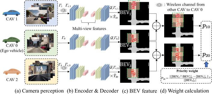
Figure 4: Procedure for priority weight calculation. Fig. 4(a): CAVs observe surroundings with 4 cameras; CAVs 1-2 relay RGB data to CAV 0. Figs. 4(b)-(c): BEV feature generation in CAV 0. Fig. 4(d): BEV-match mechanism determines priority weights.

The procedure of calculating priority weights can be divided into three steps as follows:

(1) Camera perception: As shown in Fig. 4(a), the nearby CAVs capture raw camera data $\varGamma$ using its four cameras. This perception data $\varGamma$ is then transmitted to the ego CAV by communication units through wireless channel. Let $\varGamma_{t}=\mathcal{F}(\varGamma)$ denote the perception data received by the ego CAV, where $\mathcal{F}$ represents the function of data transmission over the network. In reality, different data processing strategies result in different impacts on $\varGamma_{t}$, such as compression and transmission latency.

(2) Encoder & Decoder: Fig. 4(b) illustrates that upon reception, the ego CAV uses a SinBEVT-based neural network to process the single-vehicle’s RGB data[6]. This data is transformed through an encoding-decoding process to extract BEV features. The BEV feature transformation is denoted by $\text{BEV}=\mathcal{G}(\varGamma_{t})$, where $\mathcal{G}$ captures SinBEVT’s processing essence. In Fig. 4(c), the BEV feature depicts the traffic scenario from a single vehicle’s perspective, with the green dashed box marking the range of perceived moving vehicles, and the red box indicating surrounding vehicles to the ego CAV. In fact, SinBEVT and CoBEVT achieve real-time performance of over 70 fps with five CAVs[6].

(3) Priority weight calculation: As shown in Fig. 4(d), we take the ego CAV and CAV 1 as an example. Along with their corresponding BEV perceptions $\text{BEV}_{0}$ and $\text{BEV}_{1}$, let the coordinates and orientation angle of both the Ego CAV and CAV 1 be represented as $(x_{0},y_{0},\theta_{0})$ and $(x_{1},y_{1},\theta_{1})$, respectively. Firstly, we can derive the translational displacement between Ego CAV and CAV 1: $\Delta x=x_{0}-x_{1}$, $\Delta y=y_{0}-y_{1}$ and $\Delta\theta=\theta_{0}-\theta_{1}$. Accordingly, the translation matrix $T$ and the rotation matrix $\varTheta$ are articulated as:

$$T_{10}=\left[\begin{matrix}1&0&\Delta x\\ 0&1&\Delta y\\ 0&0&1\\ \end{matrix}\right],\varTheta_{10}=\left[\begin{matrix}\cos\mathrm{(}\Delta\theta)&-\sin\mathrm{(}\Delta\theta)&0\\ \sin\mathrm{(}\Delta\theta)&\cos\mathrm{(}\Delta\theta)&0\\ 0&0&1\\ \end{matrix}\right],$$ (10)

where $\hat{T}_{10}=T_{10}\times\varTheta_{10}$ remap coordinates from $\text{BEV}_{1}$ to $\text{BEV}_{0}$. Let $\hat{\varGamma}$ be a point of the BEV feature of CAV 1. Furthermore, the transformation of a point $\hat{\varGamma}$ from the BEV perception $\text{BEV}_{1}$ to $\text{BEV}_{0}$ is denoted by $\hat{\varGamma}^{\prime}=\hat{T}_{10}\times\hat{\varGamma}$. $\hat{\varGamma}^{\prime}$ represents the transformed coordinate in $\text{BEV}_{0}$ and the point $\hat{\varGamma}$ is articulated in homogeneous coordinates, i.e., $\hat{\varGamma}=[x,y,1]^{T}$. Inspired by the definition of IoU, we design a BEV-match mechanism, which exploits BEV-match level as the priority weight. Specifically, the priority weight $\mathcal{P}_{10}$ is formulated as follows:

$$\mathcal{P}_{10}=\frac{\|[\mathrm{BEV}_{0}\cap\mathrm{BEV}_{1}^{\prime}]_{\pi}-[\mathrm{BEV}_{0}]_{\pi}\|_{2}}{|[\mathrm{BEV}_{0}]_{\pi}|},$$ (11)

where $\text{BEV}_{\text{0}}$ denote the ego CAV’s BEV features and $\text{BEV}_{1}^{\prime}=\hat{T}_{10}\times\text{BEV}_{1}$ signifies the transformed BEV, the operation $[\cdot]_{\pi}$ zeros pixels outside the largest bounding rectangle of the fused BEV’s non-zero region, $\|\cdot\|_{2}$ measures the square root of squared pixel values, $|\cdot|$ sums all pixel values in an image, and the numerator in Eq. (11) quantifies perception difference between data from CAVs 1 and 0, with the denominator providing normalization. The term $\mathcal{P}$ in fact captures two characteristics between the view of the ego CAV and the transformed view of the assisting CAV for data fusion. If two views are very close, the intersection will be similar, the numerator in Eq. (11) will be very small, thus ${\mathcal{P}}_{10}$ will be very small, which implies that the view from CAV 1 will not be helpful to enhance the perception quality, meaning that the view from CAV 1 can be assigned low priority. If the view from CAV 1 is too dissimilar, the intersection will be close to empty, implying that the numerator in Eq. (11) will be close to 1, meaning that the view from CAV 1 may be more helpful and should be assigned higher priority.

4.3 Utilization Maximization in Collaborative Perception

The performance of collaborative perception relies on the quality of the V2V communication network. Hence, our aim is to maximize the amount of perception data transmitted under the constraints of communication resources, such as power and bandwidth. However, given the varying contributions of nearby CAVs, it is unwise to directly optimize the total throughput of the V2V networks. Instead, we employ the aforementioned priority weight to adjust the resources allocated to each CAV. Moreover, one group of CAVs might have overlapping perceptual regions, so it is intuitive to leverage the set of the union-style perception region $G_{i}$ as the factor of perception performance, which can be given by $G_{i}=\bigcup_{j\in J_{i}}{\mathcal{G}_{j}}$, where ${\mathcal{G}_{j}}$ denotes the perception region by the $j$th CAV and $J_{i}=\{j|s_{ji}=1\}$. Let $\mathcal{I}\left(\mathcal{S}_{i}\right)$ represent the total area covered by the union of perceptual regions of vehicles in set $J_{i}$, we can define

$$\mathcal{I}\left(\mathcal{S}_{i}\right)=\mathcal{A}\left(\bigcup_{j\in J_{i}}{\mathcal{G}_{j}}\right),$$ (12)

where $\mathcal{A}(X)$ returns the area of a region $X$. Specifically, given the priority weight $\mathcal{P}$, and the link establishment set $\mathcal{S}$, the sub-utility function for the perception quality is formulated as $\mathcal{U}_{\mathrm{r}}=\sum_{i}\sum_{j=1,j\neq i}{{\mathcal{P}}_{ji}s_{ji}d_{ji}}$, which indicates the accuracy and robustness of surrounding perception. While $\mathcal{U}_{\mathrm{p}}=\sum_{i}\mathcal{I}\left(\mathcal{S}_{i}\right)$ denotes the sub-utility function of the perceptual regions of CAVs, which represents the amount of information collected by data fusion. To maximize both utilities at the same time, the weighted utility function is formulated as:

$$\mathcal{U}_{\mathrm{sum}}(\mathcal{S},\mathcal{D}) =\mathrm{\omega}_{1}\mathcal{U}_{\mathrm{r}}+\mathrm{\omega}_{2}\mathcal{U}_{\mathrm{p}}$$ (13)

$$=\mathrm{\omega}_{1}\underset{\text{Perception quality}}{\underbrace{\sum_{i=1}^{N}{\sum_{j=1,j\neq i}^{N}{\mathcal{P}_{ji}s_{ji}d_{ji}}}}}+\mathrm{\omega}_{2}\underset{\text{Perceptual region}}{\underbrace{\sum_{i=1}^{N}{\mathcal{I}\left(\mathcal{S}_{i}\right)}}},$$

where $\omega_{1}$ and $\omega_{2}$ denote the weights of perception quality and perceptual region, respectively. The optimized variable $\mathcal{D}=\left[d_{ij}\right]_{N\times N}$ is the matrix of data transmission rate. By combining the constraints and objective function Eq. (13), we formulate the utility function maximization problem as:

$$\mathbf{P}: \max\limits_{\mathcal{\mathcal{R}},\mathcal{S},\mathcal{D}}\quad\mathcal{U}_{\mathrm{sum}}(\mathcal{S},\mathcal{D})$$ (14)

s.t. $$(\ref{eq:subchannel}),(\ref{eq:transmission rate}),(\ref{eq:the constraint of the compression ratio}),(\ref{eq:the constraint of the compression ratio 2}),(\ref{eq:computing power constraint}),(\ref{eq:power constraint}),$$

where the constraint (2) is the upper bound of the number of subchannels; (3) denotes the constraint of transmission rate; (4) and (5) are the constraints of the compression ratio; (7) and (9) are the upper bounds of the computing capacity and transmission power, respectively. In Sec. 5, we prove that the utility function maximization can be decomposed into two problems, i.e., a nonlinear programming problem and submodular optimization problem that can be solved by a greedy algorithm with an approximation guarantee.

5 Two-Stage Optimization Framework for Utility Maximization

In this section, we first want to show that the original problem $\mathbf{P}$ is NP-hard, making it hard to find its optimal solution within latency-sensitive systems. To find a suboptimal solution, we conceive a two-stage optimization framework, which decomposes $\mathbf{P}$ into two distinct problems: a nonlinear programming (NLP) $\mathbf{P_{1}}$, and a submodular optimization $\mathbf{P_{2}}$. We ascertain the optimal solution for $\mathbf{P_{1}}$ in Sec. 5.1, and deduce a $(1-e^{-1})$-approximation of the optimal value for $\mathbf{P_{2}}$ using an iterative algorithm in Sec. 5.3.

5.1 Nonlinear Programming Problem Analysis

Proposition 1:

For fixed $\mathcal{D}^{(n)}$, problem $\mathbf{P}$ is reducible from Weighted Maximum Coverage Problem (WMCP). When optimizing over matrices $\mathcal{D}$ and $\mathcal{R}$, $\mathbf{P}$ surpasses WMCP’s complexity, establishing its NP-hardness.

Proof:

Define the Weighted Maximum Coverage Problem (WMCP) with universe $U$, subset family $\mathcal{F}=\left\{\hat{S}_{1},\ldots,\hat{S}_{F}\right\}$, and weight function $w:U\rightarrow\mathbb{R}_{\geq 0}$. For set $\hat{S}\subseteq U$ and subset family $\mathcal{Y}\subseteq\mathcal{F}$:

$$w(\hat{S})=\sum_{u\in\hat{S}}w(u),$$

where $w(\mathcal{Y})=w\left(\bigcup_{\hat{S}\in\mathcal{Y}}\hat{S}\right)$. WMCP aims to select subsets from $\mathcal{F}$ to maximize the weight of their elements:

$$\max_{\hat{S}}\sum_{u\in\hat{S}}w(u)\quad\text{s.t.}\quad\left|\hat{S}\right|<K,\hat{S}_{f}\subseteq U.$$ (15)

According to the definition of the utility function in Eq. (13), we define the weight function with fixed $\mathcal{D}^{(n)}$ as follows:

$$\mathcal{U}_{i}(\mathcal{S}_{i},\mathcal{D}^{(n)})=\mathrm{\omega}_{1}\sum_{j=1,j\neq i}^{N}{\mathcal{P}_{ji}s_{ji}d_{ij}^{(n)}}+\mathrm{\omega}_{2}\mathcal{I}\left(\mathcal{S}_{i}\right).$$ (16)

It is noted that each element in $U$ is a unique link for a CAV in $\mathbf{P}$. The weight $w$ in WMCP aligns with the utility $\mathcal{U}_{i}(\mathcal{S}_{i},\mathcal{D}^{(n)})$ in $\mathbf{P}$. Hence, with fixed $\mathcal{D}^{(n)}$, the problem can be seen as WMCP. Considering the optimization over $\mathcal{D}$ and $\mathcal{R}$, $\mathbf{P}$ extends beyond WMCP, introducing complexities from $\mathcal{D}$ and $\mathcal{R}$. Given the inherent NP-hardness of WMCP and the added complexity when including optimization over $\mathcal{D}$ and $\mathcal{R}$, we can infer that problem $\mathbf{P}$ is, at the very least, as hard as the classical WMCP. Hence, problem $\mathbf{P}$ is NP-hard. $\blacksquare$

According to Proposition 1, it can be concluded that the problem $\mathbf{P}$ is NP-hard. Besides, it can be observed that as the number of cooperative vehicles $N$ increases, the state space of problem $\mathbf{P}$ exhibits double exponential growth. Specifically, with the state space represented as $2^{\left(N^{2}\right)}\times\mathcal{D}_{n}\times\mathcal{R}_{n}$, the dimensionality increases rapidly with respect to $N$. For example, let $\mathcal{D}_{n}$ and $\mathcal{R}_{n}$ denote the discrete levels for continuous variables $\mathcal{D}$ and $\mathcal{R}$. We can consider a scenario with 10 CAVs (refer to Sec. 6.2). As for the upper bound of $\mathcal{D}$ is $40$ Mbps, we assume a step size of 1 Mbps with a total of $\mathcal{D}_{n}=40$ levels. As for the compression ratio $\mathcal{R}$, there are also $\mathcal{R}_{n}=20$ levels with an increment of 0.05 per level. Therefore, we can obtain the state space of the problem $\mathbf{P}$ is approximately $1.014\times 10^{33}$.

It is highly complicated to find the optimal solution even when the V2V network scale is no more than $10$ vehicles. Since the control and decision of CAVs are latency-sensitive, we have to conceive a real-time optimization solver to address the issue of finding an optimal solution for the NP-hard problem $\mathbf{P}$. Therefore, we decompose $\mathbf{P}$ into two subproblems by fixing one of the optimization variables.

Denote the link establishment in the $n$th round as $\mathcal{S}^{(n-1)}$. We then focus on adjusting the matrices for the compression ratio $\mathcal{R}$ and the data rate $\mathcal{D}$. Problem $\mathbf{P}_{1}$ is expressed as:

$$\mathbf{P_{1}}: \max\limits_{\mathcal{R},\mathcal{D}}\ \ \mathcal{U}_{\mathrm{sum}}\left(\mathcal{S}^{(n-1)},\mathcal{D}\right)$$ (17)

s.t. $$(\ref{eq:transmission rate}),(\ref{eq:the constraint of the compression ratio}),(\ref{eq:the constraint of the compression ratio 2}),$$

$$(\ref{OP:P1}\textrm{a}):A_{j}+\sum_{i=1,i\neq j}^{N}{{r}_{ij}s_{ij}^{(n-1)}d_{ij}}\leqslant F_{j}/\beta,$$

$$(\ref{OP:P1}\textrm{b}):\sum_{i=1,i\neq j}^{N}\left(E_{j}^{t}\big{|}_{s_{ij}^{(n-1)}}+E_{ij}^{c}\big{|}_{s_{ij}^{(n-1)}}\right)\leq E^{T}_{j}.$$

For $j=1,2,\ldots,N$, the sub-problem $\mathbf{P}_{1}$ is an NLP problem due to the nonlinear constraints given by (3), (17a), and (17b). While global optimization techniques like branch and bound or genetic algorithms can be used for non-convex problems, they are computationally demanding. Our approach is to linearize the problem. We define $\mathbf{U}=\mathcal{R}\odot\mathcal{D}=\left[u_{ij}\right]_{N\times N}$ where $\odot$ is the Hadamard product and $u_{ij}={r}_{ij}d_{ij}$. This linearizes the product term in the constraints. Thus, $\mathbf{P}_{1}$ is reformulated as:

$$\mathbf{P}_{1-1}: \max_{\mathbf{U},\mathcal{D}}\,\,\sum_{j=1}^{N}{\sum_{i=1,i\neq j}^{N}{s_{ij}^{(n-1)}\mathcal{P}_{ij}d_{ij}}}$$ (18)

s.t. $$(\ref{OP:P1-2}\text{a}):u_{ij}\leq\min(C_{ij},A_{i}),$$

$$(\ref{OP:P1-2}\text{b}):\max({r}_{j,\min},{\eta}{e^{-L_{ij}}})\leq\frac{u_{ij}}{d_{ij}}\leq{r}_{j,\max},$$

$$(\ref{OP:P1-2}\text{c}):\sum_{i=1,i\neq j}^{N}{s_{ij}^{(n-1)}u_{ij}}\leqslant\min(\gamma_{j}^{(n-1)},\varphi_{j}),$$

where we define $\gamma_{j}^{\left(n-1\right)}$ as $\frac{E^{T}}{\epsilon_{j}\tau_{j}^{c}}-\frac{\tau_{j}^{t}P_{t}\sum_{i=1,i\neq j}^{N}{s_{ij}^{(n-1)}}}{\epsilon_{j}\tau_{j}^{c}}-A_{j}$ and $\varphi_{j}$ as $\frac{F_{j}}{\beta}-A_{j}$. Moreover, the constraint (18c) is derived from both (17a) and (17b). Even though we add a bilinear equality constraint with $u_{ij}$, constraint (18b) remains nonlinear, thereby we cannot obtain the optimal result directly. Given that $\mathbf{P_{1-1}}$ attempts to optimize $\sum_{j=1}^{N}{\sum_{i=1,i\neq j}^{N}{s_{ij}^{(n-1)}d_{ij}}}$, we have:

$$\frac{u_{ij}}{{r}_{j,\max}}\leq d_{ij}\leq\frac{u_{ij}}{\max\left({r}_{j,\min},\frac{\eta}{e^{L_{ij}}}\right)},$$ (19)

which offers an upper bound for the optimal value of $\mathbf{P_{1-1}}$. To optimize $d_{ij}$, it is beneficial to focus on maximizing this limit. Therefore, we derive a relaxed problem as follows:

$$\mathbf{P_{1-2}}: \max\limits_{\mathbf{U}}\ \ \sum_{j=1}^{N}\sum_{i=1,i\neq j}^{N}\frac{s_{ij}^{(n-1)}\mathcal{P}_{ij}u_{ij}}{\max\left({r}_{j,\min},\frac{\eta}{e^{L_{ij}}}\right)}$$ (20)

s.t. $$(\ref{OP:P1-2}\textrm{a})\ \mathrm{and}\ (\ref{OP:P1-2}\textrm{c}).$$

$\mathbf{P_{1-2}}$ is a standard linear programming solvable using techniques like the simplex or interior-point methods. If the optimal outcome of $\mathbf{P_{1-2}}$ is $u_{ij}^{(n)}$, the optimal solutions for transmission rate and adaptive compression ratio are $d_{ij}^{(n)}={u_{ij}^{(n)}}\left[{{\max\left({r}_{j,\min},\frac{\eta}{e^{L_{ij}}}\right)}}^{-1}\right]$ and ${r}_{ij}^{(n)}={u_{ij}^{(n)}}/{d_{ij}^{(n)}}$, respectively. Considering that $d_{ij}$ values are at the edges of the feasible region, the optimal solution for $\mathbf{P_{1-2}}$ matches that of $\mathbf{P_{1-1}}$.

5.2 Preliminaries for Submodular Optimization

Prior to delving into specific details of the other subproblem $\mathbf{P_{2}}$, we briefly review the definition and primary characteristics of submodularity as presented in [36].

Definition 1:

(Set Function Derivative) Given a set function $f:2^{V}\rightarrow\mathbb{R}$, for a subset $S$ of $V$ and an element $e$ in $V$, the discrete derivative of $f$ at $S$ concerning $e$ is denoted by $\Delta_{f}(e|S)$ and defined as $\Delta_{f}(e|S)=f(S\cup\{e\})-f(S)$. If the context makes the function $f$ evident, we omit the subscript, expressing it simply as $\Delta(e|S)$.

Definition 2:

(Monotonicity) Given a function $f:2^{V}\rightarrow\mathbb{R}$, $f$ is deemed monotone if, for all $A,B\subseteq V$ with $A\subseteq B$, the condition $f(A)\leq f(B)$ holds.

It should be underscored that the function $f$ exhibits monotonicity if and only if every discrete derivative maintains a non-negative value. Specifically, for each $A\subseteq V$ and any $e\in V$, the relation $\Delta(e|A)\geq 0$ is satisfied.

Definition 3:

(Submodularity) Let $E$ denote a finite ground set. A set function $f:2^{E}\rightarrow\mathbb{R}$ is said to be normalized, non-decreasing, and submodular if it satisfies the following properties:

1. $f(\emptyset)=0$;

2. $f$ is monotone as per Definition 2;

3. For any $A,B\subseteq E$, $f(A)+f(B)\geq f(A\cup B)+f(A\cap B)$;

4. For any $A\subseteq B\subseteq E$ and an element $e\in E\setminus B$, $\Delta_{f}(e|A)\geqslant\Delta_{f}(e|B)$.

In the next subsection, we prove that the objective function possesses submodular properties. As more CAVs share their perception results, the ego CAV tends to add significant new information for view fusion. However, as the number of CAV increases, each additional CAV provides less new information, i.e., Diminishing Marginal Utility. This concept is crucial in CAVs’ scenarios, ensuring that resources are not wasted by redundant sensors.

5.3 Submodular Analysis and Solutions

0:  Adaptive compression ratio matrix $\mathcal{R}^{(n)}$, data transmission rate $\mathcal{D}^{(n)}$.

10:  Output the optimal link establishment matrix $\mathcal{S}$.

1:  Initialization: $\mathcal{S}\leftarrow\emptyset$, $i\leftarrow 1$;

2:  while $i\leq N$ do

3:     $s_{ij}^{*}=\arg\max_{s_{ij}\in\mathcal{S}^{n\times n}\backslash\mathcal{S}}\mathcal{U}_{\mathrm{sum}}(\mathcal{S}\cup\{s_{ij}\},\mathcal{D}^{(n)})$;

4:     $\mathcal{S}\leftarrow\mathcal{S}\cup\{s_{ij}^{*}\}$;

5:     $i\leftarrow i+1$;

6:  end while

7:  return  $\mathcal{S}$.

Algorithm 1 Greedy Algorithm for submodular function maximization

In this subsection, we first prove that the objective function of the problem $\mathbf{P_{2}}$ is a submodular function. Specifically, as more CAVs share their perception results, the ego CAV tends to add significant new information for view fusion. However, as the number of CAV increases, each additional CAV provides less new information, i.e., Diminishing Marginal Utility. This concept is crucial in CAVs’ scenarios, ensuring that resources are not wasted by redundant sensors. Moreover, we attempt to adapt a greedy algorithm to solve the above maximization submodular function problem. Besides, we show that a greedy algorithm finds a near-optimal solution with at least $\left(1-e^{-1}\right)$ of the optimal value.

Proposition 2:

Given that $\mathbf{P}_{2}$ characterizes the link establishment problem and the data rate $\mathcal{D}=\mathcal{D}^{(n)}$ is a constant matrix, the objective function $\mathcal{U}_{\text{sum}}(\mathcal{S},\mathcal{D}^{(n)})$ defined in Eq. (13) exhibits submodularity if $\mathcal{U}_{\text{sum}}(\mathcal{S},\mathcal{D}^{(n)})$ satisfies all the properties outlined in Definition 3 within Sec. 5.2.

Proof:

Refer to four properties from Definition 3 in Sec. 5.2, we will prove that the objective function of the problem $\mathbf{P}$ satisfies all essential conditions for submodular functions as follows:

(1) To show the first property of Definition 3, we can obtain $f\left(\emptyset\right)=\mathcal{U}_{\mathrm{sum}}(\mathcal{S},\mathcal{D})=0$ if $\mathcal{S}=\mathbf{0}$, which represents that we do not establish any links so $\mathcal{S}$ is a zero matrix. Therefore, the first property of Definition 3 can be satisfied.

(2) To show the second property of Definition 3, we assume $\mathbf{B}_{1}$ and $\mathbf{B}_{2}$ are link establishment sets, where $\forall\mathbf{B}_{1}\subseteq\mathbf{B}_{2}\subseteq\mathbf{E}$. Let $\left\{s_{ij}^{\mathbf{B}_{1}}\right\}_{N\times N}$ and $\left\{s_{ij}^{\mathbf{B}_{2}}\right\}_{N\times N}$ denote the associated link establishment matrices. Thus, we have:

$$f\left(\mathbf{B}_{1}\right)=\mathcal{U}_{\mathrm{sum}}(\mathbf{B}_{1},\mathcal{D})=\sum_{i=1}^{N}{\left(\mathrm{\omega}_{1}\sum_{j=1,j\neq i}^{N}{\mathcal{P}_{ji}s_{ji}^{\mathbf{B}_{1}}d_{ij}^{(n)}}+\mathrm{\omega}_{2}\mathcal{I}\left(\mathbf{B}_{1}\right)\right)}.$$ (21)

Similarity,

$$f\left(\mathbf{B}_{2}\right)=\sum_{i=1}^{N}{\left(\mathrm{\omega}_{1}\sum_{j=1,j\neq i}^{N}{\mathcal{P}_{ji}s_{ji}^{\mathbf{B}_{2}}d_{ij}^{(n)}}+\mathrm{\omega}_{2}\mathcal{I}\left(\mathbf{B}_{2}\right)\right)}.$$ (22)

Then, let $\mathbf{B}_{2}\backslash\mathbf{B}_{1}$ represent the set of all elements that are in $\mathbf{B}_{2}$ but not in $\mathbf{B}_{1}$. Therefore, we can derive the difference between $\mathbf{B}_{1}$ and $\mathbf{B}_{2}$ as $f\left(\mathbf{B}_{2}\backslash\mathbf{B}_{1}\right)=\sum_{i=1}^{N}{\left(\mathrm{\omega}_{1}\sum_{j=1,j\neq i}^{N}{\mathcal{P}_{ji}s_{ji}^{\mathbf{B}_{2}\backslash\mathbf{B}_{1}}d_{ij}^{(n)}}+\mathrm{\omega}_{2}\mathcal{I}\left(\mathbf{B}_{2}\backslash\mathbf{B}_{1}\right)\right)}$. Each element of the matrices $s_{ij}^{\mathbf{B}}$ can only take values of 0 or 1, where 1 signifies a connected link and 0 denotes a broken or non-existent link. Given $\forall\mathbf{B}_{1}\subseteq\mathbf{B}_{2}\subseteq\mathbf{E}$, it is evident that every link connected in $\mathbf{B}_{1}$ is also connected in $\mathbf{B}_{2}$. However, the converse may not be true; there might be links in $\mathbf{B}_{2}$ that are not connected in $\mathbf{B}_{1}$. When $s_{ij}^{\mathbf{B}_{2}}=s_{ij}^{\mathbf{B}_{1}}$, the difference is zero. When $s_{ij}^{\mathbf{B}_{1}}\neq s_{ij}^{\mathbf{B}_{2}}$, the difference is positive. Therefore, the difference $f\left(\mathbf{B}_{2}\backslash\mathbf{B}_{1}\right)\geq 0$, and the objective function $\mathcal{U}_{\mathrm{sum}}(\mathcal{S},\mathcal{D})$ is monotone.

(3) To show the third property of Definition 3, we have to prove $f(\mathbf{B}_{1})+f(\mathbf{B}_{2})\geq f(\mathbf{B}_{1}\cup\mathbf{B}_{2})+f(\mathbf{B}_{1}\cap\mathbf{B}_{2})$. According to Eqs. (12) and (21), we can decompose $f(\mathcal{S}_{i})$ into two distinct components as follows:

$$f(\mathcal{S}_{i})=g(\mathcal{S}_{i})+h(\mathcal{S}_{i}),$$ (23)

where $g(\mathcal{S}_{i})=\mathrm{\omega}_{1}\mathcal{U}_{\mathrm{r}}$ is a modular function and $h(\mathcal{S}_{i})=\mathrm{\omega}_{2}\mathcal{U}_{\mathrm{p}}$ is a submodular function. As for $g(\mathcal{S}_{i})$, the modular property ensures that the sum of the values for any two subsets is equal to the sum of their union and intersection: $g(\mathbf{B}_{1})+g(\mathbf{B}_{2})=g(\mathbf{B}_{1}\cup\mathbf{B}_{2})+g(\mathbf{B}_{1}\cap\mathbf{B}_{2})$. As for $h(\mathcal{S}_{i})$, encapsulates the union of perceptual regions. The inherent property of the union operation ensures diminishing returns; adding more regions results in a lesser incremental gain, thereby making $h$ submodular. Therefore, for any $\mathbf{B}_{1},\mathbf{B}_{2}\subseteq\mathcal{S}$: $h(\mathbf{B}_{1})+h(\mathbf{B}_{2})\geq h(\mathbf{B}_{1}\cup\mathbf{B}_{2})+h(\mathbf{B}_{1}\cap\mathbf{B}_{2})$. Combining the modular and submodular components, we have $f(\mathbf{B}_{1})+f(\mathbf{B}_{2})\geq f(\mathbf{B}_{1}\cup\mathbf{B}_{2})+f(\mathbf{B}_{1}\cap\mathbf{B}_{2})$.

(4) To show the fourth property of Definition 3, we need to prove $\Delta_{f}(e|\mathbf{B}_{1})\geqslant\Delta_{f}(e|\mathbf{B}_{2})$, where $e$ is an arbitrary element in the set $\mathbf{E}\backslash\mathbf{B_{2}}$. The original inequality can be formulated as:

$$f(\mathbf{B}_{2}\cup\{e\})-f(\mathbf{B}_{1}\cup\{e\})\leqslant f(\mathbf{B}_{2})-f(\mathbf{B}_{1}).$$ (24)

Combining Eqs. (21), (22), (24) and (24), we extend the left side of the equality, which can be given by:

$$\mathcal{U}_{\mathrm{sum}}(\mathbf{B}_{1}\cap\{e\},\mathcal{D})-\mathcal{U}_{\mathrm{sum}}(\mathbf{B}_{2}\cap\{e\},\mathcal{D})$$ (25)

$$=g\left(\mathbf{B}_{2}\backslash\mathbf{B}_{1}\right)+\left[h\left(\mathbf{B}_{2}\cap\{e\}\right)-h\left(\mathbf{B}_{1}\cap\{e\}\right)\right],$$

Given that $g(\mathbf{B})$ is modular and $h(\mathbf{B})$ is submodular, it follows that $g\left(\mathbf{B}_{2}\backslash\mathbf{B}_{1}\right)=g\left(\mathbf{B}_{2}\right)-g\left(\mathbf{B}_{1}\right)$ and $h\left(\mathbf{B}_{2}\cap\{e\}\right)-h\left(\mathbf{B}_{1}\cap\{e\}\right)\leqslant h\left(\mathbf{B}_{2}\right)-h\left(\mathbf{B}_{1}\right)$ for all possible link establishment $e$. Therefore, we can obtain $\mathcal{U}_{\mathrm{sum}}(\mathbf{B}_{1}\cap\{e\},\mathcal{D})-\mathcal{U}_{\mathrm{sum}}(\mathbf{B}_{2}\cap\{e\},\mathcal{D})\leqslant g\left(\mathbf{B}_{2}\right)-g\left(\mathbf{B}_{1}\right)+h\left(\mathbf{B}_{2}\right)-h\left(\mathbf{B}_{1}\right)=\mathcal{U}_{\mathrm{sum}}(\mathbf{B}_{2},\mathcal{D})-\mathcal{U}_{\mathrm{sum}}(\mathbf{B}_{1},\mathcal{D})$. $\blacksquare$

With the adaptive compression ratio matrix $\mathcal{R}^{(n)}=\left[{r}_{ij}^{(n)}\right]_{N\times N}$ and data transmission rate $\mathcal{D}^{(n)}=\left[d_{ij}^{(n)}\right]_{N\times N}$, we then formulate the link establishment matrix $\mathcal{S}$ for $\mathbf{P}_{2}$ as:

$$\mathbf{P}_{2}: \max_{\mathcal{S}}\,\,\sum_{i=1}^{N}{\left(\mathrm{\omega}_{1}\sum_{j=1,j\neq i}^{N}{\mathcal{P}_{ji}s_{ji}d_{ij}^{(n)}}+\mathrm{\omega}_{2}\mathcal{I}\left(\mathcal{S}_{i}\right)\right)}$$ (26)

s.t. $$(\ref{OP:P2}\textrm{a}):\sum_{i=1,i\neq j}^{N}{\mathrm{\chi}_{ij}^{\left(n\right)}s_{ij}}\leq E_{j}^{T}-\tau_{j}^{c}\epsilon_{j}A_{j},$$

$$(\ref{OP:P2}\textrm{b}):\sum_{i=1,i\neq j}^{N}{s_{ij}u_{ij}^{(n)}}\leqslant\varphi_{j}\ \mathrm{and}\ (\ref{eq:subchannel}),$$

where $\mathrm{\chi}_{ij}^{\left(n\right)}=u_{ij}^{\left(n\right)}\epsilon_{j}\tau_{j}^{c}+\tau_{j}^{t}P_{t}$ can be obtained by the inequality constraint (9). Since the objective function $\mathcal{U}_{\mathrm{sum}}(\mathcal{S},\mathcal{D})$ is a submodular function according to Proposition 2, $\mathbf{P_{2}}$ is a submodular function maximization problem, which can be solved by a greedy algorithm for near-optimal results.

Proposition 3:

Given a submodular, non-decreasing set function $\mathcal{U}_{\mathrm{sum}}(\mathcal{S},\mathcal{D}^{(n)})$, which yields $\mathcal{U}_{\mathrm{sum}}(\emptyset,\mathcal{D}^{(n)})=0$, the greedy algorithm obtains a set $\mathcal{S}_{G}$ satisfying:

$$\mathcal{U}_{\mathrm{sum}}\left(\mathcal{S}_{G},\mathcal{D}^{(n)}\right)\geq\left(1-e^{-1}\right)\max_{\mathcal{S}}\mathcal{U}_{\mathrm{sum}}\left(\mathcal{S},\mathcal{D}^{(n)}\right).$$ (27)

Proof:

Please refer to Sec. II of [37]. $\blacksquare$

According to Proposition 3, it can be observed that Algorithm 1 can obtain a $(1-e^{-1})$-approximation of the optimal value of $\mathbf{P_{2}}$. During the $n$th round, we update the link establishment $\mathcal{S}^{(n)}$. If link $(i,j)$ reduces the throughput, it is removed: $\mathcal{S}^{(n)}\leftarrow\mathcal{S}^{(n)}\backslash\{s_{ij}\}$. Otherwise, it is added: $\mathcal{S}^{(n)}\leftarrow\mathcal{S}^{(n)}\cup{\{s_{ij}\}}$. For $\mathbf{P_{2}}$, we iteratively adjust links until we find an optimal solution meeting all constraints or hit the iteration limit by relying on Algorithm 1.

This greedy approach not only ensures maximization of the objective function $\mathcal{U}_{\mathrm{sum}}(\mathcal{S},\mathcal{D}^{(n)})$ but also significantly reduces computational complexity, making it highly advantageous for real-time applications. According to the cardinality constraint $K$ in (2), the time-complexity of Algorithm 1 is only $\mathcal{O}(K)$. Therefore, we can circumvent the complexities typically associated with optimization problems by such a greedy algorithm rather than engaging in exhaustive searches or iterative procedures, which may not always guarantee convergence to the optimal solution.

5.4 Deep Learning-Based Adaptive Compression

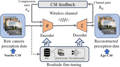
Figure 5: Overall architecture of adaptive compression.

The compression modules commonly employed in V2V collaborative networks often rely on predefined fixed compression ratios, such as JPEG and JPEG2000[6]. However, these fixed ratios are inadequate to accommodate the demands of the dynamic channel conditions discussed in Sec. 5. Moreover, it has been shown that the deep learning-based method generally offers better rate–distortion (R-D) performance compared to the standard compression methods[38]. In this section, we propose an adaptive compression method that comprises an adaptive R-D mechanism to refine the compression ratio, $\mathcal{R}$, to align with the requirements of dynamic channel conditions. Then, we introduce a fine-tuning strategy to reduce temporal redundancy in V2V transmissions by exploiting the holistic RGB frames. We first present the main procedure of our DL-based compression scheme as follows.

(1) Encoding Phase: The input image $i\in\mathbb{R}^{N}$ undergoes transformation to latent representation $h$ (expressed as $h=f(i)$). A quantization function ${Q}$ further refines $h$ into a discrete vector $q\in\mathbb{H}^{D}$, leading to $q=Q(h)$. In V2V scenarios, $q$ is serialized into bitstream $b$, with entropy coding to maximize the bandwidth efficiency.

(2) Decoding Phase: The bitstream $b$ undergoes inverse transformations. This includes dequantization ($\hat{h}=Q^{-1}(q)$) and a reconstruction function ($\hat{i}=H(\hat{h})$) to retrieve the original image. Conventional compression struggles in dynamic V2V networks due to their static nature. The Deep Learning-Based Compression (DBC) addresses this by trainable parameters from training datasets, thus offering adaptability to V2V dynamics. Under DBC architecture, both encoder and decoder utilize convolutional layers. The encoder transforms the input image into a latent representation, $h=f_{\theta}(i)$, with transformation parameters $\theta$ learned from training. The decoder uses a distinct parameter set $\xi$ for reconstruction: $\hat{i}=H_{\xi}(h)$. The training objective is to minimize:

$$\mathop{\arg\min}_{\theta,\xi}R\left(b\right)+\beta D(i,\hat{i}),$$ (28)

where $R(b)$ and $D(i,\hat{i})$ measure bitrate and distortion using the Mean Square Error (MSE). Constant $\beta$ manages the R-D trade-off. Moreover, we formulate the traditional fixed R-D problem as a multi-R-D problem for adaptability:

$$\mathop{\arg\min}_{\theta,\xi}R(\hat{h};\theta)+\beta D\left(i,\hat{i};\theta,\xi\right),$$ (29)

Notably, a static $\beta$ can affect reliable decoding and image quality, emphasizing the need to adjust $\beta$ adaptively. In this context, we introduce a DBC mechanism to dynamically modify $\beta$ under dynamic channel conditions (As shown in Fig. 5, given the channel state information (CSI) feedback, we can obtain $\beta$ and compression ratio according to Sec. 5.1). Therefore, the revised problem can be formulated as:

$$\mathop{\arg\min}_{\theta,\xi}R(\hat{h};\theta,{r})+G({r})D\left(i,\hat{i};\theta,\xi,{r}\right).$$ (30)

It is noted that the adaptive compression network is based on a pre-trained model[25], using historical camera data as training dataset to obtain network parameter $\theta,\xi$ by solving the multi-R-D problem in (30).

(3) Fine-tuning Phase: This adaptive approach enables the ego CAV and nearby CAVs adaptively adjust the data compression ratio according to dynamic channel conditions. As shown in Fig. 5, we introduce a fine-tuning compression strategy to further reduce temporal redundancy between frames. Utilizing a Modulated Autoencoder (MAE), our method first transmits a few uncompressed images to RSU for real-time fine-tuning. As for computational cost, the encoder and decoder of MAE require 0.155 MFLOPs/pixel and 0.241 MFLOPs/pixel, respectively[25]. Considering Tesla FSD as the computational unit, when three CAVs share their perception results at a rate of 10 fps, the average latencies for encoding and decoding processes are observed to be 40.26 ms and 20.89 ms, respectively.

0:  Multi-CAV data $\varGamma$, number of vehicles $N$, channel parameter constraints $K,C_{ij}$, device parameters ${r}_{j,\min},{r}_{j,\max},\eta,\tau_{j}^{t},\tau_{j}^{c},E_{j}^{T}$, etc.

0:  Priority weight $\mathcal{P}$, near-optimal compression ratio $\mathcal{R}$, link establishment $\mathcal{S}$, data rate $\mathcal{D}$, modulated autoencoder, and BEV prediction.

1:  Calculate priority weight $\mathcal{P}$ according to Sec. 4;

2:  Initialize the link establishment decision $\mathcal{S}^{(0)}$;

3:  for $j=0$ to $N-1$ do

4:     Sort column in descending order and get the indices of the largest $K$ capacity, and set the associated $s_{ij}=1$;

5:  end for

6:  while Convergence not achieved do

7:     Solve the linear programming problem $\mathbf{P_{1-2}}$;

8:     Solve the submodular problem $\mathbf{P_{2}}$ using Algorithm 1;

9:  end while

10:  Obtain the near-optimal solution for $\mathcal{R},\mathcal{S},\mathcal{D}$;

11:  Determine the trade-off parameter $\beta^{*}$ based on the channel state;

12:  According to Eq.( 30), train encoders (decoders) to compress (reconstruct) raw camera data;

13:  Predict BEV feature using the reconstructed camera data.

Algorithm 2 Priority Aware Collaborative Perception

6 Simulation Results and Discussions

In this section, we evaluate our schemes under various communication settings, which consist of bandwidth, transmission power, the number of CAVs, and the distribution of vehicles. Subsequently, we delve into the comparison of raw data reconstruction performance—both with and without the application of a fine-tuned compression strategy. In the final part of this section, we present the results of BEV along with the associated IoU.

6.1 Dataset and Baselines

Dataset: To validate our approach, we employ the CARLA and OpenCOOD simulation platforms, exploiting the OPV2V dataset[28]. This dataset encompasses 73 varied scenes, a multitude of CAVs, 11,464 frames, and in excess of 232,000 annotated 3D vehicle bounding boxes. All of these have been amassed using the CARLA simulator[27].

Baseline 1: the Fairness Transmission Scheme (FTS), which is built on the principles laid out in [26]. The cornerstone of this approach is the allocation of subchannels in a manner that resonates with Jain index defined in Eq. (1).

Baseline 2: The core of this baseline is the Distributed Multicast Data Dissemination Algorithm (DMDDA), as outlined in [21], which seeks to optimize throughput in a decentralized fashion.

Baseline 3: the No Fusion scheme, which implies the usage of a single ego vehicle for gathering information about its surroundings. It operates without integrating data from the cameras of proximate CAVs.

To ensure a fair comparison, we maintain uniformity in the transmission model and simulation parameters, aligning them to those discussed in Sec. 3.2.

6.2 Simulation Settings

Our simulations are based on the 3GPP standard[32]. Specifically, the communication range for vehicles is 150 m. Vehicular speeds, unless otherwise stated, ranging from $0$ to $50$ km/h (typical speed range on city roads), are generated using the CARLA simulator[27]. Additionally, vehicles are uniformly distributed over a six-lane highway of 200 meters, with three lanes allocated for each traveling direction. To simplify, certain frame types, such as cyclic redundancy checks and Reed-Solomon coding, have been omitted from our simulation. In our simulation setup, we consider a system with $N=10$ cooperative vehicles. Each vehicle has local data of $A_{j}=40$ Mbits and can access up to $K=4$ subchannels. The computation complexity is quantified by $\beta=100$ Cycles/bit, and each vehicle transmits at a power $P_{t}=8$ mW. The CPU capacity, $F_{j}$, of these vehicles varies between 1 GHz and 3 GHz, as highlighted by Lyu et al. in [21]. Additionally, we allocate a bandwidth of $W=200$ MHz and set a power threshold $E_{j}^{T}=1$ kW for each vehicle.

6.3 Analysis of Experimental Results

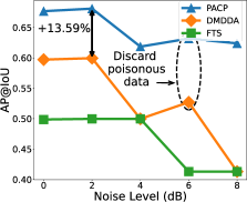
(a) IoU vs. Noise level

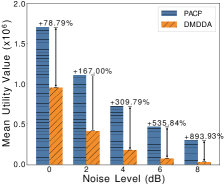
(b) Utility vs. Noise level

Figure 6: AP@IoU and utility value under different noise levels.

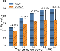
(a) $\mathcal{U}_{\mathrm{sum}}$ vs. Power

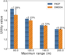
(b) $\mathcal{U}_{\mathrm{sum}}$ vs. $R_{\max}$

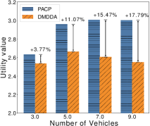
(c) $\mathcal{U}_{\mathrm{sum}}$ vs. CAV num.

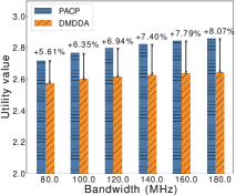
(d) $\mathcal{U}_{\mathrm{sum}}$ vs. Bandwidth

Figure 7: Results on average utility value $\mathcal{U}_{\mathrm{sum}}$ under different communication settings.

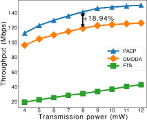
(a) Throughput vs. Power

(b) Throughput vs. $R_{\max}$

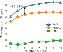
(c) Throughput vs. CAV num.

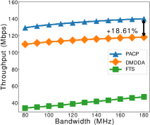
(d) Throughput vs. Bandwidth

Figure 8: Results on average network throughput under different communication settings.

In our study, we evaluate the efficacy of the proposed PACP algorithm in maximizing utility value and enhancing perception accuracy (AP@IoU). We benchmark its performance against two established methods: DMDDA[21] and FTS[26]. For fairness, all evaluations are carried out under consistent conditions. Firstly, we conducted experiments to investigate the impact of electromagnetic interference on collaborative perception. The interference levels were classified based on their relative noise floor according to urban environment: 0 dB over -174 dBm/Hz (Low), 4 dB over -174 dBm/Hz (Medium), and 8 dB over -174 dBm/Hz (High). As illustrated in Fig. 6, perception accuracy and utility value deteriorate sharply as noise level intensifies. While PACP outperforms both DMDDA and FTS in terms of AP@IoU. Specifically, PACP shows an improvement of 14.04% over DMDDA and 36.58% over FTS, because PACP utilizes the adaptive compression to reduce packet loss and latency. In Fig. 6(a), due to the priority-aware scheme, PACP effectively discards poisonous data, thereby mitigating interference adverse impact on perception. In Fig. 6(b), PACP demonstrates superior performance compared to DMDDA in terms of utility value by increasing over 78.79%.

In Eq. (13), the utility value $\mathcal{U}_{\mathrm{sum}}$ denotes the weighted utility function of perception quality and perceptual region. As the priority value is determined by the degree of IoU matching, a larger utility value indicates that more data matching the perception results of the ego CAV have been transmitted. Intuitively, the higher the utility value, the higher the accuracy of the perception results of the ego CAV. Fig. 7 presents a comprehensive view of how different communication parameters influence the utility value $\mathcal{U}_{\mathrm{sum}}$. In Fig. 7(a), as the transmission power increases, both PACP and DMDDA show an improvement in the utility value. However, the utility value of PACP consistently surpasses that of DMDDA. Specifically, at a typical power 8.0 mW, PACP is about 8.27% better than DMDDA, underlining the efficiency of the proposed PACP approach over the baseline in terms of better prioritized data communication. Fig. 7(b) indicates that the utility value generally declines as the maximum range increases. Despite this trend, PACP consistently outperforms DMDDA, illustrating its robustness even when the communication range is extended. Fig. 7(c) reveals that as the number of CAVs increases, the utility value increases. After deploying 9 vehicles, the PACP algorithm outstrips DMDDA by a notable margin of 17.79%. This accentuates the scalability and efficacy of PACP in larger vehicular networks. From Fig. 7(d), PACP amplifies the utility value by 8.07% in comparison with DMDDA at a bandwidth of 180 MHz. This suggests that PACP is adept at capitalizing on larger bandwidths to enhance the perception accuracy of the ego CAV.

Intuitively, we can adopt throughput as a metric for cooperative perception. Similar to utility value, a higher throughput often entails a greater amount of valuable information being transmitted. Fig. 8(a) shows that larger power enhances throughput. Fig. 8(b) depicts an inverse correlation between the vehicle distribution maximum range (80 m - 210 m) and throughput. It is noted that the performance of FTS strategy deteriorates because of balancing communication channels of remote vehicles. Remarkably, with five cooperative CAVs, the PACP algorithm augments the average throughput by 20.39% compared with DMDDA. Furthermore, Fig. 8(d) underscores the linear affinity between the network’s bandwidth (80-180 MHz) and throughput. Specifically, a bandwidth of $W=180$ MHz elevates the average throughput by 18.61% using the PACP algorithm against other baselines. To sum up, it is evident that a higher throughput results in a richer amount of high-priority data being transmitted according to Figs. 7-8.

TABLE II: The comparison of PACP with three baselines under different parameters in terms of perception accuracy.

	Power (mW)			Num. of CAVs			Bandwidth (MHz)
	5	8	11	2	3	4	80	140	200
No Fusion	0.408	0.408	0.408	0.408	0.408	0.408	0.408	0.408	0.408
FTS	0.410	0.499	0.499	0.506	0.447	0.410	0.410	0.410	0.499
DMDDA	0.590	0.605	0.646	0.648	0.605	0.603	0.597	0.597	0.603
PACP	0.662	0.673	0.684	0.685	0.685	0.685	0.672	0.680	0.685
Improvement	12.20%	11.24%	5.88%	5.71%	13.22%	13.60%	12.56%	13.90%	13.60%

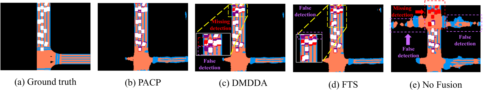
Figure 9: BEV prediction: (a) Ground Truth, (b) PACP, (c) DMDDA, (d) No Fusion. PACP accurately detects dynamic objects, unlike DMDDA, FTS, and No Fusion. White: correct detection; Red: missing detection; Purple: false detection.

To further analyze the performance of perception accuracy, we conduct extensive experiments to verify the performance of PACP. From Table II, it is evident that the proposed PACP method consistently outperforms other techniques under various settings. PACP, underpinned by a priority-aware perception scheme, demonstrates a remarkable increase in perception accuracy, surpassing FTS by a minimum of 35.38% and DMDDA by 5.71% in scenarios under varying numbers of CAVs. Given a typical bandwidth 200 MHz, the improvement of adapting PACP achieves up to 13.60%. Such performance elevation is attributed to PACP’s adeptness at channel allocation based on CAVs’ significance to the ego vehicle, ensuring optimal transmission of pivotal perception data. Contrarily, fairness-based strategies, as exemplified by FTS’s bandwidth-fairness and DMDDA’s subchannel-fairness, inadvertently lead to suboptimal resource allocation by treating every CAV with uniform significance. This often results in the situation that vital information receives the same resource allocation as non-essential data, consequently diminishing AP@IoU and increasing the chances of missed detections in a BEV context. Not unexpectedly, as the power, the number of CAVs, and bandwidth increase, the amount of information perceived by the ego CAV expands, leading to a consequent rise in the AP@IoU for all perception strategies.

Fig. 9 illustrates the BEV predictions across different schemes, setting an emphasis on the deviations from the Ground truth (GT), depicted in Fig. 9(a), which symbolizes the paragon of collaborative perception communication. Observing Fig. 9(b), the PACP stands out by registering zero false or missing detections, adhering closely to GT. On the other hand, DMDDA and FTS schemes, represented in Figs. 9(c) and (d), manifest a notable number of missing detections, highlighting the inefficacies in their perception algorithms. The most striking deviations are observed in the No Fusion scheme, as portrayed in Fig. 9(e). This scheme, relying solely on single vehicle perception, results in an escalated number of both false and missing detections. Such stark disparities accentuate the imperativeness of leveraging multi-view data fusion for optimized perception outcomes and further illuminate the pronounced efficacy of the PACP scheme over its contemporaries.

7 Conclusions

In this paper, we have investigated the perception challenges posed by the inherent limitations of the BEV, particularly its blind spots, in ensuring the safety and reliability of connected and autonomous vehicles. We have introduced the novel PACP framework that leverages a unique BEV-match mechanism, discerning priority levels by computing the correlation between the captured information from nearby CAVs and the ego vehicle. By employing a two-stage optimization based on submodular optimization, PACP optimally regulates transmission rates, link connectivity, and compression metrics. A distinguishing feature of PACP is its integration with a deep learning-based adaptive autoencoder, which is further enhanced by fine-tuning mechanisms, ensuring efficient image reconstruction quality under dynamic channel conditions. Evaluations conducted on the CARLA platform with the OPV2V dataset have confirmed the superiority of PACP to existing methodologies. The results have demonstrated that PACP improves the utility value and AP@IoU by 8.27% and 13.60%, respectively, highlighting its potential to set new benchmarks in the realm of collaborative perception for connected and autonomous vehicles.

References

- [1] S. Hu, Z. Fang, Y. Deng, X. Chen, and Y. Fang, “Collaborative perception for connected and autonomous driving: Challenges, possible solutions and opportunities,” arXiv preprint arXiv:2401.01544, 2024.
- [2] S. Hu, Z. Fang, H. An, G. Xu, Y. Zhou, X. Chen, and Y. Fang, “Adaptive communications in collaborative perception with domain alignment for autonomous driving,” arXiv preprint arXiv:2310.00013, 2023.
- [3] S. Hu, Z. Fang, X. Chen, Y. Fang, and S. Kwong, “Towards full-scene domain generalization in multi-agent collaborative bird’s eye view segmentation for connected and autonomous driving,” arXiv preprint arXiv:2311.16754, 2023.
- [4] X. Chen, Y. Deng, H. Ding, G. Qu, H. Zhang, P. Li, and Y. Fang, “Vehicle as a service (VaaS): Leverage vehicles to build service networks and capabilities for smart cities,” arXiv preprint arXiv:2304.11397, 2023.
- [5] Y. Xiao, F. Codevilla, A. Gurram, O. Urfalioglu, and A. M. López, “Multimodal end-to-end autonomous driving,” IEEE Transactions on Intelligent Transportation Systems, vol. 23, no. 1, pp. 537–547, Aug. 2022.
- [6] R. Xu, Z. Tu, H. Xiang, W. Shao, B. Zhou, and J. Ma, “CoBEVT: Cooperative bird’s eye view semantic segmentation with sparse transformers,” in Conference on Robot Learning (CoRL), Auckland, NZ, Dec. 2022.
- [7] Y. Zhang, H. An, Z. Fang, G. Xu, Y. Zhou, X. Chen, and Y. Fang, “SmartCooper: Vehicular collaborative perception with adaptive fusion and judger mechanism,” in IEEE International Conference on Robotics and Automation (ICRA), Yokohama, Japan, May 2024.
- [8] Y. Yuan, H. Cheng, and M. Sester, “Keypoints-based deep feature fusion for cooperative vehicle detection of autonomous driving,” IEEE Robotics and Automation Letters, vol. 7, no. 2, pp. 3054–3061, Jan. 2022.
- [9] M. Noor-A-Rahim, Z. Liu, H. Lee, M. O. Khyam, J. He, D. Pesch, K. Moessner, W. Saad, and H. V. Poor, “6G for vehicle-to-everything (V2X) communications: Enabling technologies, challenges, and opportunities,” Proceedings of the IEEE, vol. 110, no. 6, pp. 712–734, May 2022.
- [10] Y.-C. Liu, J. Tian, N. Glaser, and Z. Kira, “When2com: Multi-agent perception via communication graph grouping,” in IEEE/CVF Conference on Computer Vision and Pattern Recognition (CVPR), Seattle, WA (Virtual), 2020, pp. 4106–4115.
- [11] Z. Wang, Z. Zhang, J. Wang, C. Jiang, W. Wei, and Y. Ren, “AUV-assisted node repair for IoUT relying on multi-agent reinforcement learning,” IEEE Internet of Things Journal, (DOI: 10.1109/JIOT.2023.3298522), 2023.
- [12] A. Geiger, P. Lenz, and R. Urtasun, “Are we ready for autonomous driving? The KITTI vision benchmark suite,” in IEEE Conference on Computer Vision and Pattern Recognition (CVPR), Providence, RI, Jul. 2012, pp. 3354–3361.
- [13] Q. Chen, X. Ma, S. Tang, J. Guo, Q. Yang, and S. Fu, “F-cooper: Feature based cooperative perception for autonomous vehicle edge computing system using 3D point clouds,” in Proceedings of the 4th ACM/IEEE Symposium on Edge Computing, Arlington, Virginia, Nov. 2019, pp. 88–100.
- [14] T.-H. Wang, S. Manivasagam, M. Liang, B. Yang, W. Zeng, and R. Urtasun, “V2VNet: Vehicle-to-vehicle communication for joint perception and prediction,” in European Conference on Computer Vision (ECCV), Glasgow, United Kingdom, Aug. 2020, pp. 605–621.
- [15] J. Li, R. Xu, X. Liu, J. Ma, Z. Chi, J. Ma, and H. Yu, “Learning for vehicle-to-vehicle cooperative perception under lossy communication,” IEEE Transactions on Intelligent Vehicles, vol. 8, no. 4, pp. 2650–2660, Mar. 2023.
- [16] S. Wang, Y. Hong, R. Wang, Q. Hao, Y.-C. Wu, and D. W. K. Ng, “Edge federated learning via unit-modulus over-the-air computation,” IEEE Transactions on Communications, vol. 70, no. 5, pp. 3141–3156, Feb. 2022.
- [17] A. Skodras, C. Christopoulos, and T. Ebrahimi, “The JPEG 2000 still image compression standard,” IEEE Signal Processing Magazine, vol. 18, no. 5, pp. 36–58, Sep. 2001.
- [18] H. Liu, H. Yuan, Q. Liu, J. Hou, and J. Liu, “A comprehensive study and comparison of core technologies for MPEG 3-D point cloud compression,” IEEE Transactions on Broadcasting, vol. 66, no. 3, pp. 701–717, Dec. 2020.
- [19] Q. Chen, S. Tang, Q. Yang, and S. Fu, “Cooper: Cooperative perception for connected autonomous vehicles based on 3d point clouds,” in IEEE 39th International Conference on Distributed Computing Systems (ICDCS), Dallas, TX, Oct. 2019, pp. 514–524.
- [20] Z. Y. Rawashdeh and Z. Wang, “Collaborative automated driving: A machine learning-based method to enhance the accuracy of shared information,” in 21st International Conference on Intelligent Transportation Systems (ITSC), Maui, Hawaii, Dec. 2018, pp. 3961–3966.
- [21] X. Lyu, C. Zhang, C. Ren, and Y. Hou, “Distributed graph-based optimization of multicast data dissemination for internet of vehicles,” IEEE Transactions on Intelligent Transportation Systems, vol. 24, no. 3, pp. 3117–3128, Dec. 2022.
- [22] B. L. Nguyen, D. T. Ngo, N. H. Tran, M. N. Dao, and H. L. Vu, “Dynamic V2I/V2V cooperative scheme for connectivity and throughput enhancement,” IEEE Transactions on Intelligent Transportation Systems, vol. 23, no. 2, pp. 1236–1246, Sep. 2022.
- [23] Y. Ma, W. Liang, J. Wu, and Z. Xu, “Throughput maximization of NFV-enabled multicasting in mobile edge cloud networks,” IEEE Transactions on Parallel and Distributed Systems, vol. 31, no. 2, pp. 393–407, 2020.
- [24] S. Zhang, J. Chen, F. Lyu, N. Cheng, W. Shi, and X. Shen, “Vehicular communication networks in the automated driving era,” IEEE Communications Magazine, vol. 56, no. 9, pp. 26–32, Sep. 2018.
- [25] F. Yang, L. Herranz, J. Van De Weijer, J. A. I. Guitián, A. M. López, and M. G. Mozerov, “Variable rate deep image compression with modulated autoencoder,” IEEE Signal Processing Letters, vol. 27, pp. 331–335, Jul. 2020.
- [26] E. R. Magsino and I. W.-H. Ho, “An enhanced information sharing roadside unit allocation scheme for vehicular networks,” IEEE Transactions on Intelligent Transportation Systems, vol. 23, no. 9, pp. 15 462–15 475, Jan. 2022.
- [27] A. Dosovitskiy, G. Ros, F. Codevilla, A. Lopez, and V. Koltun, “CARLA: An open urban driving simulator,” in Conference on robot learning (CoRL), Mountain View, California, Nov. 2017, pp. 1–16.
- [28] R. Xu, H. Xiang, X. Xia, X. Han, J. Li, and J. Ma, “OPV2V: An open benchmark dataset and fusion pipeline for perception with vehicle-to-vehicle communication,” in International Conference on Robotics and Automation (ICRA), Philadelphia, PA, May 2022, pp. 2583–2589.
- [29] Y. Yu, T. Wang, and S. C. Liew, “Deep-reinforcement learning multiple access for heterogeneous wireless networks,” IEEE Journal on Selected Areas in Communications, vol. 37, no. 6, pp. 1277–1290, Jun. 2019.
- [30] M. Adil, H. Song, J. Ali, M. A. Jan, M. Attique, S. Abbas, and A. Farouk, “Enhanced-AODV: A robust three phase priority-based traffic load balancing scheme for internet of things,” IEEE Internet of Things Journal, vol. 9, no. 16, pp. 14 426–14 437, Apr. 2022.
- [31] X. Luo and P. Li, “Learning-based off-chain transaction scheduling in prioritized payment channel networks,” IEEE Journal on Selected Areas in Communications, vol. 40, no. 12, pp. 3589–3599, Oct. 2022.
- [32] W. Anwar, N. Franchi, and G. Fettweis, “Physical layer evaluation of V2X communications technologies: 5G NR-V2X, LTE-V2X, IEEE 802.11bd, and IEEE 802.11p,” in IEEE 90th Vehicular Technology Conference (VTC2019-Fall), Honolulu, HI, Sep. 2019, pp. 1–7.
- [33] M. Adil, H. Song, J. Ali, M. A. Jan, M. Attique, S. Abbas, and A. Farouk, “Enhanced-AODV: A robust three phase priority-based traffic load balancing scheme for internet of things,” IEEE Internet of Things Journal, vol. 9, no. 16, pp. 14 426–14 437, Apr. 2021.
- [34] Z. Xiao, Z. Han, A. Nallanathan, O. A. Dobre, B. Clerckx, J. Choi, C. He, and W. Tong, “Antenna array enabled space/air/ground communications and networking for 6G,” IEEE Journal on Selected Areas in Communications, vol. 40, no. 10, pp. 2773–2804, Aug. 2022.
- [35] W. Chen, X. Lin, J. Lee, A. Toskala, S. Sun, C. F. Chiasserini, and L. Liu, “5G-Advanced toward 6G: Past, present, and future,” IEEE Journal on Selected Areas in Communications, vol. 41, no. 6, pp. 1592–1619, Jun. 2023.
- [36] S. Dobzinski and J. Vondrák, “Communication complexity of combinatorial auctions with submodular valuations,” in Twenty-Fourth Annual ACM-SIAM Symposium on Discrete Algorithms, 2013, pp. 1205–1215.
- [37] A. Krause and D. Golovin, “Submodular function maximization.” Tractability, vol. 3, no. 71-104, p. 3, 2014.
- [38] J. Ballé, V. Laparra, and E. P. Simoncelli, “End-to-end optimized image compression,” in International Conference on Learning Representations (ICLR), Toulon, France, Apr. 2017, pp. 1–27.