Solvable toy model of negative energetic elasticity
Abstract
Recent experiments have established negative energetic elasticity, the negative contribution of energy to the elastic modulus, as a universal property of polymer gels. To reveal the microscopic origin of this phenomenon, Shirai and Sakumichi investigated a polymer model on a cubic lattice with the energy effect from the solvent in finite-size calculations [Phys. Rev. Lett. 130, 148101 (2023)]. Motivated by this work, we provide a simple platform to study the elasticity of polymer chains by considering a one-dimensional random walk with the energy effect. This model can be mapped onto the classical Ising chain, leading to an exact form of the free energy in the thermodynamic or continuous limit. Our analytical results are qualitatively consistent with Shirai and Sakumichi’s work. Our model serves as a fundamental benchmark for studying negative energetic elasticity.
Introduction.— In condensed matter physics, solvable toy models play a crucial role in understanding the essence of phenomena. For instance, entropic elasticity, which explains the elastic modulus of rubbers, appears in a one-dimensional (1D) random walk. This serves as a concrete example to comprehend how the number of possible states is converted into elasticity through statistical mechanics [1, 2].
Rubberlike materials consist of polymer chains that form entangled and crosslinked networks. The elastic modulus of rubberlike materials is determined not only by the entropic contribution but also by the energetic one. Experiments with natural and synthetic rubbers have demonstrated that the energetic contribution is negligibly small [3, 4, 5]. Consequently, the energy effect has been ignored in the well-known theories of rubber elasticity [6, 7, 8, 9]. However, recent experiments have revealed a significant negative energetic contribution in polymer gels, which are composed of polymer networks containing a large amount of solvent [10, 11, 12, 13, 14, 15]. Understanding the microscopic origins of negative energetic elasticity remains an important problem.
To address this issue, several approaches have been proposed. Shirai and Sakumichi investigated a 3D self-avoiding walk, a random walk that does not overlap with itself, by conducting an exact enumeration [16]. The self-avoiding walk is acknowledged as an effective lattice model for a single polymer chain in a dilute solution since it reproduces the excluded volume phenomena of polymers [17]. The energy effect from solvents was initially discussed in Ref. [18] and later improved to the so-called interacting self-avoiding walk [19]. Shirai and Sakumichi treated the self-repulsive interactions of this model and derived negative energetic elasticity. In another research, Bleha and Cifra employed the Monte Carlo method to study a continuum wormlike chain [20], which represents the polymer chain as a continuous curve and gives energy as the integral of curvature [21]. This model describes semiflexible polymers characterized by high energy costs for bending such as a double-stranded DNA [22]. They found a negative energetic contribution to force at moderate extension, which decreases with higher extension. Additionally, Hagita et al. conducted all-atom molecular dynamics simulations on polyethylene glycol hydrogels [23], which was used in the first observation of negative energetic elasticity [10]. They performed these simulations under both constant-volume and constant-pressure conditions and confirmed that the former shows stronger negativity in energetic elasticity. As a more recent work, Duarte and Rizzi proposed a simple model, a 1D random walk with independent energy at each step [24]. This model is trivially solvable because it is non-interacting.
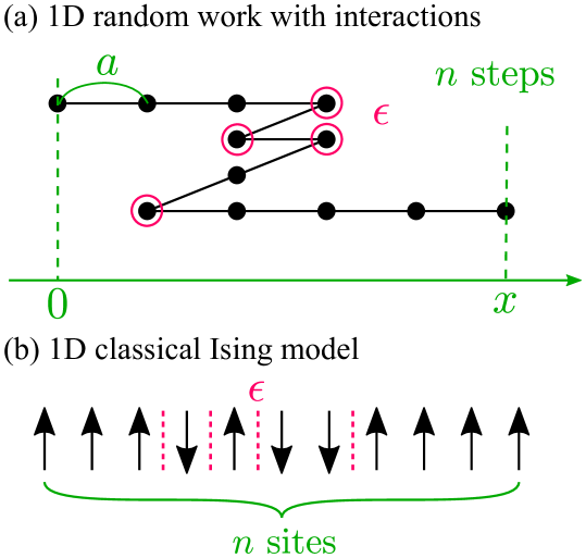
There is a need for an interacting model that can be analytically solved in the thermodynamic limit because previous approaches rely on finite-size computations, numerical simulations, or a non-interacting model. In this Letter, we propose a toy model to study negative energetic elasticity by introducing an energy cost to each bend in a 1D random walk as shown in Fig. 1(a). This model can be mapped onto the 1D classical Ising model depicted in Fig. 1(b), resulting in an exact solution in the thermodynamic or continuous limit. The energy cost at each bending behaves as a self-repulsive interaction like Shirai and Sakumichi’s work on a self-avoiding walk [16], and as a result, this model exhibits negative energetic elasticity. Our results are a natural extension of entropic elasticity in a 1D random walk, thus we believe that this model will be fundamental to explain the elasticity of polymer gels.
Model.— We start with a 1D random walk characterized by the number of steps , the width per step , and the final position as shown in Fig. 1(a). To incorporate the energy effect, we introduce an energy term for each bending. For instance, the realization depicted in Fig. 1(a) incurs an energy cost of . By associating right (left) steps with up (down) spins, this model can be mapped onto the 1D classical Ising model as shown in Fig. 1(b). Therefore, the Hamiltonian of this model is given by
| (1) |
where is the classical spin at site , representing the right/left direction of -th step. With an external force , the whole Hamiltonian becomes
| (2) |
because the final position is expressed by the spins as . These Hamiltonians express the 1D classical Ising model with and without a magnetic field up to an energy constant. Our model is a 1D version of a discrete wormlike chain [25] which is equivalent to the classical XY model.
In the following, we exactly calculate the thermodynamic functions under two independent conditions; the external force is fixed in the first and the final position is fixed in the second. The first case is described by the Ising model in a magnetic field, whereas the second case is described by the Ising model with a fixed magnetization. The force-fixed and position-fixed conditions correspond to the constant-pressure and constant-volume condition of all-atom molecular dynamics in Ref. [23], respectively. Under both conditions, we can obtain the relationship between and by differentiating the thermodynamic functions. This relationship allows us to calculate the stiffness , which represents the elastic modulus of a single chain, along with its energetic and entropic contributions.
Force-fixed condition.— We need to consider all possible realizations of a random walk with an external force , which means all configurations of the Hamiltonian described by Eq. (2). Consequently, the partition function at a temperature is given by
| (3) |
This partition function can be represented by the transfer matrix as
| (4) |
where
| (5) |
From the largest eigenvalue of , the Gibbs free energy, the thermodynamic function under this condition, can be calculated as
| (6) |
The relationships between and is determined through as
| (7) |
where is the rescaled dimensionless position . The stiffness can be calculated as a function of and .
| (8) |
Here, we have introduced rescaled dimensionless quantities and .
In order to decompose the stiffness into its energetic and entropic contributions as [10], we consider the Helmholtz free energy , which is the thermodynamic function under the position-fixed condition calculated in the next part. Since we can obtain by the differentiation of as , the stiffness is given by . Considering that is decomposed into the energetic and entropic term as , the energetic and entropic contributions to the stiffness can be defined as and , respectively. By applying Maxwell’s relation, both contributions can be computed from as and .
In the simplest case with , the stiffness and its energetic and entropic contributions are derived from Eq. (8) as
| (9) |
where and are rescaled dimensionless quantities. Therefore, when the interactions are repulsive (), the energetic contribution becomes negative (), indicating negative energetic elasticity. As will be plotted later, the behavior of Eq. (9) is qualitatively consistent with Fig. 3 of Ref. [16] on a self-avoiding walk.
In the vicinity of a temperature , the stiffness is approximated by
| (10) |
Therefore, in experiments and numerical simulations, when the stiffness is lineally approximated as , a dimensionless quantity
| (11) |
is used as an indicator of negative energetic elasticity. We can analytically obtain in the limit of as
| (12) |
indicating that negative energy elasticity diminishes as the chain is extended. This result is consistent with the previous work on a wormlike chain [20].
Position-fixed condition.— The position-fixed condition corresponds to the Ising model with a fixed magnetization, where the partition function is given by
| (13) |
We categorize the summation based on the number of bends as
| (14) |
where is the number of cases of -bending realizations with the final position of a -step random walk. Since does not depend on the sign of , we have . Denoting the number of right and left steps as
| (15) |
and assuming , i.e., , is evaluated by division into four cases: the random walks starting with the right/left step and ending with the right/left step. Therefore, we obtain the partition function as
| (16) |
To evaluate the summation, we insert a Kronecker delta in an integral form,
| (17) |
where is a counterclockwise contour around the origin. By carrying out the summation, we obtain the partition function in an integral form as
| (18) |
This representation also holds when because the change of the variable confirms . Applying the saddlepoint approximation, we obtain the Helmholtz free energy, the thermodynamic function under this condition, as
| (19) |
From the differentiation of this function as , we can derive the relationship between and , which is equivalent to Eq. (7). This is because the Helmholtz free energy contains the same information as the Gibbs free energy . These two thermodynamic functions are connected to each other through the Legendre transformation,
| (20) | |||
| (21) |
Numerical demonstrations.— Here, we examine our analytical results and compare them to finite-size numerical simulations with under the force-fixed and position-fixed conditions.
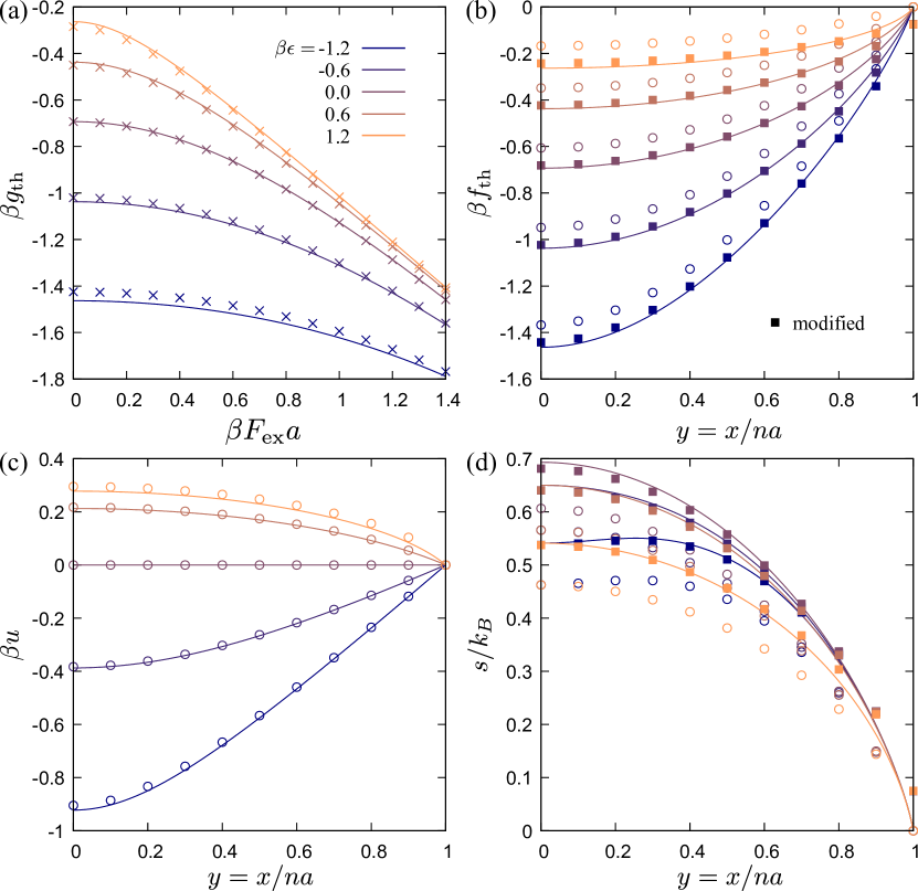
Figures 2(a) and (b) show the thermodynamic functions under both conditions in Eqs. (6) and (19). Under the force-fixed condition, the equilibrium value of is determined by maximizing following Eq. (21). Thus, the Gibbs free energy is convex upward as seen in Fig. 2(a). On the other hand, the equilibrium value of is obtained by minimizing following Eq. (20) under the position-fixed condition, resulting in a convex downward behavior of the Helmholtz free energy as illustrated in Fig. 2(b). The data points in Fig. 2(a) are consistent with the analytical results. However, in Fig 2(b), the raw numerical data represented by circle points differs from the exact solutions due to the finite-size effect. Detailed calculation of the saddle point approximation in Eq. (19) allows us to evaluate the dominant term of this finite-size effect as
| (22) |
This dominant term , which is independent of and , does not affect energy, external force, and stiffness. We modify the numerical results by subtracting the dominant term from the finite-size calculations of the free energy. The modified numerical results shown as square dots in Fig. 2(b) are in improved agreement with the exact solutions.
We decompose the Helmholtz free energy into the energy and entropy as shown in Figs. 2(c) and (d). Because the energetic and entropic contributions to the stiffness are determined by the second derivative of these quantities, the convexity observed in Figs. 2(c) and (d) characterizes each contribution to elasticity. When the interaction is repulsive as , displays upward convexity, indicating negative energetic elasticity. In the self-attractive case with , the entropy becomes convex downward near at low temperature, which means negative entropic elasticity. After removing the finite-size effect according to Eq. (22), the numerical results are in good agreement with the exact solutions.
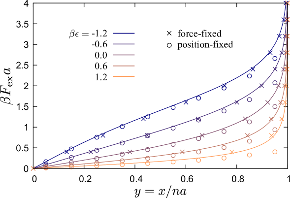
The relationship between the external force and final position in Eq. (7) is plotted in Fig. 3. The numerical data are generated by differentiating the thermodynamic functions shown in Figs. 2(a) and (b). For the position-fixed condition, is approximated using a finite difference form as
| (23) |
where . As expected, the stronger force is required to extend the chain for the larger . The numerical results under the force-fixed condition show good agreement with the exact solutions across the whole range, while discrepancies arise at high extensions under the position-fixed condition. This is because the finite-size effect depends on the ensemble used; it is exponentially small in the force-fixed condition and polynomially small in the position-fixed condition.
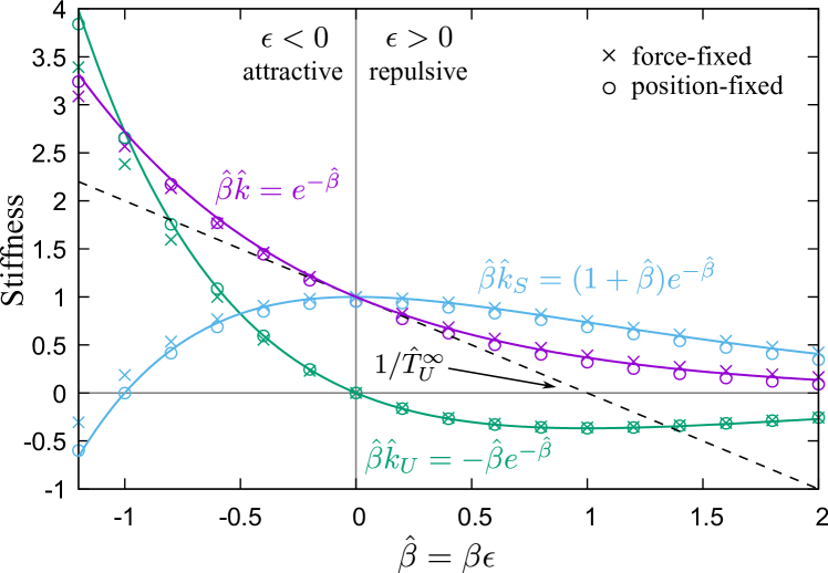
Figure 4 displays the stiffness and its energetic and entropic contributions at in Eq. (9). The numerical data are derived from the second derivative of the thermodynamic functions shown in Figs. 2(a) and (b) at or , employing a finite-difference form for the position-fixed case as
| (24) |
We observe negative energetic elasticity in the self-repulsive region with and negative entropic elasticity in the self-attractive and low-temperature region, which aligns with the convexity seen in Figs. 2(c) and (d). The dashed line represents the tangent line of at . This line crosses the horizontal axis at , which is determined analytically in Eq. (12); in this case with , . The numerical results are almost coincident with the exact solutions for both conditions. The qualitative behavior of Fig. 4 is consistent with those reported in Fig. 3 of Ref. [16] on a self-avoiding walk.
Summary and discussions.— We have proposed a toy model to explore negative energetic elasticity, a 1D random walk with an energy cost for each bending. This model can be mapped onto the 1D classical Ising model by associating right (left) steps with up (down) spins. Table 1 shows how these models correspond. We have exactly calculated the thermodynamic functions under the force-fixed and position-fixed conditions in Eqs. (6) and (19) using the transfer-matrix formulation and saddlepoint approximation. The Legendre transformation connects these thermodynamic functions as they are equivalent. We analytically obtained the stiffness in Eq. (8), which has a negative energetic contribution when the interaction is repulsive as .
| Random walk | Ising model |
|---|---|
| right/left step | up/down spin |
| external force | magnetic field |
| final position | magnetization |
| stiffness |
Our model reproduces several properties of previous studies on negative energetic elasticity. The stiffness and its energetic and entropic contributions in the simplest case in Eq. (9) plotted in Fig. 4 are qualitatively consistent with the results of a 3D self-avoiding walk in Fig. 3 of Ref. [16]. Equation (12) shows that the negative energetic contribution decreases compared to the entropic one with chain extension, in accordance with Ref. [20] for a continuum wormlike chain. The force-fixed and position-fixed conditions of our model correspond to the constant-pressure and constant-volume conditions of all-atom molecular dynamics simulations in Ref. [23]. Therefore, the finite-size effect in these simulations may resemble our model. In this sense, our model serves as an essential platform for investigating the elasticity of polymer chains.
We can extend our model to -dimensional space with . In this space, steps in each direction are mapped onto one of possible states arranged in a line and the energy cost for bending becomes interactions between different states adjacent to each other. This framework leads to the -state Potts model in 1D, which can be also analytically solved under the fixed-force condition using the transfer matrix method.
Acknowledgments.— We thank Yuta Sakai for comments on the Ising model. We are also grateful to Naoyuki Sakumichi and Hidehiro Saito for fruitful discussions. A. I. and S. O. were supported by a Grant-in-Aid for JSPS Research Fellow (Grant No. 21J21992, 22KJ0988).
References
- Kittel [1969] C. Kittel, Thermal Physics (Wiley, New York, 1969).
- Kubo [1988] R. Kubo, Statistical Mechanics: An Advanced Course with Problems and Solutions (North-Holland Physics, New York, 1988).
- Meyer and Ferri [1935] K. H. Meyer and C. Ferri, Sur l’élasticité du caoutchouc, Helvetica Chimica Acta 18, 570â589 (1935).
- Anthony et al. [1942] R. L. Anthony, R. H. Caston, and E. Guth, Equations of state for natural and synthetic rubber-like materials. I. unaccelerated natural soft rubber, The Journal of Physical Chemistry 46, 826â840 (1942).
- Mark [1976] J. E. Mark, Thermoelastic results on rubberlike networks and their bearing on the foundations of elasticity theory, Journal of Polymer Science: Macromolecular Reviews 11, 135â159 (1976).
- Flory [1953] P. J. Flory, Principles of Polymer Chemistry (Cornell University Press, Ithaca, 1953).
- James and Guth [1953] H. M. James and E. Guth, Statistical thermodynamics of rubber elasticity, The Journal of Chemical Physics 21, 1039â1049 (1953).
- Flory [1969] P. J. Flory, Statistical Mechanics of Chain Molecules (Wiley Interscience, New York, 1969).
- Flory [1977] P. J. Flory, Theory of elasticity of polymer networks. the effect of local constraints on junctions, The Journal of Chemical Physics 66, 5720â5729 (1977).
- Yoshikawa et al. [2021] Y. Yoshikawa, N. Sakumichi, U.-i. Chung, and T. Sakai, Negative energy elasticity in a rubberlike gel, Phys. Rev. X 11, 011045 (2021).
- Sakumichi et al. [2021] N. Sakumichi, Y. Yoshikawa, and T. Sakai, Linear elasticity of polymer gels in terms of negative energy elasticity, Polymer Journal 53, 1293â1303 (2021).
- Fujiyabu et al. [2021] T. Fujiyabu, T. Sakai, R. Kudo, Y. Yoshikawa, T. Katashima, U.-i. Chung, and N. Sakumichi, Temperature dependence of polymer network diffusion, Phys. Rev. Lett. 127, 237801 (2021).
- Aoyama and Urayama [2023] T. Aoyama and K. Urayama, Negative and positive energetic elasticity of polydimethylsiloxane gels, ACS Macro Letters 12, 356â361 (2023).
- Tang et al. [2023a] J. Tang, R. H. Colby, and Q. Chen, Revisiting the elasticity of tetra-poly(ethylene glycol) hydrogels, Macromolecules 56, 2939â2946 (2023a).
- Tang et al. [2023b] J. Tang, X. Duan, and Q. Chen, Temperature dependence of the gel modulus depends on change of solvent quality, Macromolecules 56, 8574â8580 (2023b).
- Shirai and Sakumichi [2023] N. C. Shirai and N. Sakumichi, Solvent-induced negative energetic elasticity in a lattice polymer chain, Phys. Rev. Lett. 130, 148101 (2023).
- Madras and Slade [1996] N. Madras and G. Slade, The Self-Avoiding Walk (Birkhäuser Boston, 1996).
- Orr [1947] W. J. C. Orr, Statistical treatment of polymer solutions at infinite dilution, Transactions of the Faraday Society 43, 12 (1947).
- Vanderzande [1998] C. Vanderzande, Lattice Models of Polymers (Cambridge University Press, 1998).
- Bleha and Cifra [2022] T. Bleha and P. Cifra, Energy/entropy partition of force at DNA stretching, Biopolymers 113 (2022).
- Kratky and Porod [1949] O. Kratky and G. Porod, Röntgenuntersuchung gelöster fadenmoleküle, Recueil des Travaux Chimiques des Pays-Bas 68, 1106â1122 (1949).
- Broedersz and MacKintosh [2014] C. P. Broedersz and F. C. MacKintosh, Modeling semiflexible polymer networks, Rev. Mod. Phys. 86, 995 (2014).
- Hagita et al. [2023] K. Hagita, S. Nagahara, T. Murashima, T. Sakai, and N. Sakumichi, All-atom molecular dynamics simulations of poly(ethylene glycol) networks in water for evaluating negative energetic elasticity, Macromolecules 56, 8095â8105 (2023).
- Duarte and Rizzi [2023] L. K. R. Duarte and L. G. Rizzi, On the origin of the negative energy-related contribution to the elastic modulus of rubber-like gels, The European Physical Journal E 46 (2023).
- Rosa et al. [2003] A. Rosa, T. X. Hoang, D. Marenduzzo, and A. Maritan, Elasticity of semiflexible polymers with and without self-interactions, Macromolecules 36, 10095â10102 (2003).