A scalable 2-local architecture for quantum annealing of all-to-all Ising models

Abstract

Achieving dense connectivities is a challenge for most quantum computing platforms today, and a particularly crucial one for the case of quantum annealing applications. In this context, we present a scalable architecture for quantum annealers defined on a graph of degree $d=3$ and containing exclusively 2-local interactions to realize an all-to-all connected Ising model. This amounts to an efficient braiding of logical chains of qubits which can be derived from a description of the problem in terms of triangles. We also devise strategies to address the challenges of scalable architectures, such as the faster shrinking of the gap due to the larger physical Hilbert space, based on driver Hamiltonians more suited to the symmetries of the logical solution space. We thus show an alternative route to scale up devices dedicated to classical optimization tasks within the quantum annealing paradigm.

Introduction - Quantum annealing (QA) [1, 2, 3] is an analog form of quantum computation which encodes the solution to a certain problem in the ground state of a final Hamiltonian $H_{f}$. This is done by preparing the ground state of a trivial Hamiltonian $H_{0}$ and interpolating towards $H_{f}$ following

$$H(t)=(1-\lambda(t))H_{0}+\lambda(t)H_{f},$$ (1)

where $\lambda(0)=0$ and $\lambda(t_{f})=1$ with $t_{f}$ being the total time of the anneal.

An interesting Hamiltonian in the context of annealing applications is the Ising model

$$H_{\text{ising}}=H_{f}=\sum_{i}h_{i}\sigma^{z}_{i}+\sum_{j>i}J_{ij}\sigma^{z}_{i}\sigma^{z}_{j},$$ (2)

which is relatively simple to implement in a number of quantum computing platforms, such as superconducting quantum circuits [4, 5] or neutral atoms [6, 7]. The cost function of many relevant classical problems can be cast in the shape of (2), often requiring all-to-all interactions. However, establishing a dense connectivity among all qubits remains a challenging task, since the hard-wiring of all the necessary links is not scalable due to crosstalk and packing issues within the chip. Based on [8], it was proposed in [9, 10] to make up for the required connectivity by establishing chains of qubits that represent the same logical variable. This is then implemented in a fixed family of graphs within which one searches for an optimal embedding, an approach known as minor embedding. Another alternative [11] is switching to the description of the problem in terms of parities between the original variables. This allows to encode the original cost function into single-qubit terms at the expense of additional 4- and 3-body interactions (or 2-local interactions mediated by qutrits), which are harder to achieve experimentally (however, some proposals do exist [12]). Recently, a new method based on perturbative gadgets has been proposed for realizing all-to-all connectivity [13], but which comes at the cost of interaction strengths of $\mathcal{O}(N^{6})$ for an $N$-qubit problem.

In this letter, we provide a novel architecture that enables the encoding of arbitrary Ising models, while requiring only 2-local interactions, where every qubit is linked to other 3 qubits at most. We develop this architecture step by step from a decomposition of the original problem in terms of triads of qubits, and in doing so we naturally arrive at a family of alternative formulations of the original problem of independent interest, which were previously pointed out in [14, 15].

Triangle decomposition of the Ising problem - In order to kick-start the description of our encoding organically, we first consider the less general class of $\mathbb{Z}_{2}$-symmetric classical Ising models for a system of size $N$, described as:

$$H_{\mathbb{Z}_{2}}=\sum_{i,j}J_{ij}\sigma^{z}_{i}\sigma^{z}_{j}$$ (3)

The starting point of this construction is the fact that the energy of an all-to-all connected Hamiltonian of the shape (3) can be described as the sum of the energies of single triangles with edges $j^{\triangle}_{ij}$, as long as $J_{ij}=\sum_{\triangle\supset\{i,j\}}j^{\triangle}_{ij}$.

$$H_{\mathbb{Z}_{2}}=\sum_{\triangle}H_{\triangle}$$ (4)

$$H_{\triangle}=j^{\triangle}_{ij}\sigma^{z}_{i}\sigma^{z}_{j}+j^{\triangle}_{ik}\sigma^{z}_{i}\sigma^{z}_{k}+j^{\triangle}_{jk}\sigma^{z}_{j}\sigma^{z}_{k}\text{ for }\{i,j,k\}\subset\triangle$$ (5)

$q_{0}q_{1}$	$00$	$01$	$10$	$11$
$l_{0}l_{1}l_{2}$	$000$, $111$	$110$, $001$	$011$, $100$	$101$, $010$

$q_{0}q_{1}$	$00$		$01$		$10$		$11$
$q_{2}$	$0$	$1$	$0$	$1$	$0$	$1$	$0$	$1$
$l_{0}l_{1}l_{2}$	$000$	$111$	$110$	$001$	$011$	$100$	$101$	$010$

Table 1: Encoding of logical triangle configurations ($l_{i}$ variables) in physical spins ($q_{i}$) for the $\mathbb{Z}_{2}$-symmetric case (a) and non-symmetric case (b) including local fields, which includes an additional sign qubit $q_{2}$.

To describe the encoding of triangular cells we employ 2 qubits, since this is enough to describe the energetically distinct states of the model due to inversion symmetry. This is illustrated in Table 1a.

Without loss of generality, we adopt the convention of always labeling the all-parallel configuration as “00”. In the following description, we refer to the space in which we are representing triangles in terms of pairs of spins as the physical representation, while the original model is referred to as the logical representation.

We can determine the Hamiltonian $H_{\triangle}^{\text{physical}}$ acting on a physical qubit pair that reproduces the correct energies by solving a simple $4\times 4$ linear system. Following Table 1a. we find:

$$H_{\triangle}^{\text{physical}}=h_{0}\sigma^{z}_{q_{0}}+h_{1}\sigma^{z}_{q_{1}}+J\sigma^{z}_{q_{0}}\sigma^{z}_{q_{1}}$$ (6)

$$\text{where}\qquad h_{0}=j_{01},\qquad h_{1}=j_{02},\qquad J=j_{12}.$$ (7)

Consistency conditions among triangles - In order to ensure that the separate triangular cells refer to a logical state in the original model, we enforce some constraints. These can be deduced from the realization that shared edges among triangles, also referred to as interacting edges from here on, must be consistent with each other: if the configuration of one cell is such that the shared edge holds parallel spins, this must also be the case for other triangular cells that contain said edge. It is easy to check that, for the encoding illustrated in Table. 1a., this can always be achieved by the means of strong 2-local ferromagnetic interactions, as long as every cell has at least one edge that is not shared with any other cell. This non-interacting edge is labeled with the “11” configuration in order to avoid the need for many-body terms. With this, the full physical Hamiltonian embedding the logical problem is:

$$H_{p}=\sum_{\triangle}H_{\triangle}^{\text{physical}}+H_{\text{constraints}}$$ (8)

$$H_{\text{constraints}}=\sum_{p\in\{\triangle\}}\sum_{\begin{subarray}{c}q\in\{\triangle\}\\ q>p\end{subarray}}J_{P}(I-\sigma^{z}_{p_{i}}\sigma^{z}_{q_{j}})$$ (9)

where $i,j$ can be 0 or 1 depending on the internal labeling of the triangular cell configurations. For sufficiently strong ferromagnetic penalties $J_{P}$, the Hamiltonian (8) exactly encodes the spectrum of the original $H_{\mathbb{Z}_{2}}$ in its low-energy eigenspace. We note that the generation of strong enough ferromagnetic interactions as system size grows is an issue that presents itself in all penalty-enforced embedding. Some studies on the scalability of penalties have been carried out for the minor embedding and LHZ cases, showing linear [16, 17] and up to quadratic [17] penalty growth in the range of problems and system sizes examined; similar results are expected for the present scheme due to its similarities with them. We tackle this limitation further on in this paper by proposing driver Hamiltonians that ease these penalty strength requirements.

Scaling up the construction - For an arbitrary graph of size $N$ we can always find some family of decompositions in terms of triangles such that every edge is accounted for at least once, and such that all triangles hold a non-interacting edge. This is achieved by choosing all the triangles such that they have a selected node $k^{*}$ in common. Starting from a single triangular cell, the graph can be increased from size $\eta$ to $\eta+1$ according to this criterion as follows: for the addition of each new node $i=\eta+1$, we include the triangles that complete the missing links to restore full connectivity by selecting the triads $\{i,k,k^{*}\}$, where $k=1,...,k^{*}-1,k^{*}+1,...,\eta$ is one of the remaining older nodes. With this scheme, the addition of an $\eta$-th qubit adds $\eta-2$ new triangles, and thus $2(\eta-2)$ physical qubits, such that the total number of qubits $n$ required by the physical implementation is:

$$n=2\sum_{\eta=1}^{N-2}\eta=(N-1)(N-2)$$ (10)

To complete the algorithmic formulation of the construction, we consider the inclusion of the full coupling strength between two qubits in the first triangular cell where it appears, and set it to zero in the following triangular cells that contain said edge. We note that this choice is valid because it satisfies the condition $J_{ij}=\sum_{\triangle}j^{\triangle}_{ij}$. With this, the procedure to build the full hardware graph can be rephrased as follows. First, we choose the selected node $k^{*}$, i.e., the logical variable to be involved in all the triangles. Then, we arrange the pairs of physical qubits representing triangular cells as follows: the first (top-most) row contains the cell $(0,1,k^{*})$, with $k^{*}$ being the selected node, the second row contains $(0,2,k^{*})$ and $(1,2,k^{*})$, etc., skipping over $k^{*}$. The resulting graph is illustrated in Fig. 1 for the case of $N=5$ and $k^{*}=2$. Following the consistency conditions previously described, we end up with strong ferromagnetic links connecting neighboring cells that share an edge in such a way that every physical qubit is connected to at most other 3, taking into account the link that connects the pair of physical qubits within each cell.

Incorporation of local fields - We can simulate a general Ising model like the one in Eq. (2) by slightly modifying the current construction: due to the symmetry breaking, now an additional physical qubit is required for the description of each triangle. We refer to the latter as a sign qubit, and it indicates whether the parallel spins are pointing upwards or downwards (represented by $q_{2}$ in Table 1b.). The single-cell Hamiltonian giving the right energy contributions can be found by solving the $8\times 8$ linear system, in accordance with what was done in the $\mathbb{Z}_{2}$-symmetric case.

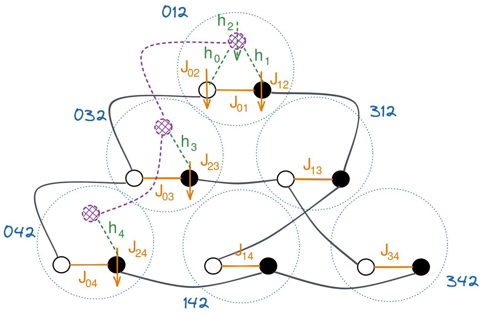
FIG. 1: Full hardware graph representing a sparse realization of Eq. (2) for $N=5$, which also corresponds to a sparse realization of Eq. (3) for $N=5$ in the absence of the sign qubits. Blue dotted circles group the qubits representing a single cell, corresponding to the triad of qubits in blue closest to it. The purple dashed links correspond to strong ferromagnetic connections among sign qubits. Orange and (dashed) green color-coding corresponds to the $\{J_{ij}\}$ and $\{h_{i}\}$ of the logical problem. In this illustration, $k^{*}=2$.

The consistency conditions regarding sign qubits imply that they are ferromagnetically coupled to the sign qubits of their neighboring cells. However, following again the rule of including the full local field on the first appearance, the only sign qubits that maintain some connectivity with the rest of their cell are those corresponding to the left-most diagonal. Thus, the remaining sign qubits are expendable and can be spared by collapsing ferromagnetic links. The resulting scheme is illustrated for $N=5$ in Fig. 1.

We highlight that if the logical chains are allowed to be of length $N-1$ instead of $N-2$, the incorporation of local fields can be done within the same structure as the one described in the absence of local fields.

Driver Hamiltonians for scalability - Two issues arise when embedding a problem within a larger Hilbert space by means of some constraints: the preservation of the logical ground state as the ground state of $H_{p}$ (which amounts to enforcing the constraints strongly enough) and the scaling of the minimal gap, since it now decreases with the physical system size $n$ rather than the original logical system size $N$. The standard driver Hamiltonian for annealing $H_{0}=H_{std}=-\sum_{i}\sigma^{x}_{i}$ encodes no information about the feasible solution subspace, and is thus expected to render a search through a space much larger than necessary. This makes the computation less efficient and translates into an exponentially decreasing minimal gap in comparison to the fully connected model. This was also pointed out in the SQA study benchmarking the performance of minor embedding vs. LHZ in [18].

However, we do have information about the relevant subspace to explore: it is the space spanned by $\{|0\rangle^{\otimes l},|1\rangle^{\otimes l}\}$ within each chain, which we will refer to as the logical subspace $\mathcal{L}$. The collection of optimal driver Hamiltonians for the annealing of $H_{p}$ should thus commute with the operator $P$ describing the restriction to this subspace [20, 21], i.e., $[P,H_{0}]=[P,H_{p}]=0$, $[H_{0},H_{p}]\neq 0$ and also induce hopping between all regions of the solution space. Notice that for our architecture $P=\sum_{c_{k}\in\mathcal{C}}\sum_{i\in c_{k}}\sigma^{z}_{i}\sigma^{z}_{i+1}$. These conditions automatically solve both of the previously described issues by removing the need for constraints and making the annealing of the embedded problem equivalent to that of the fully connected model. However, a Hamiltonian of these characteristics for the class of $H_{p}$ at hand will have highly nonlocal terms , rendering its physical implementation impractical.

In order to find more feasible alternatives, we relax the previous conditions such that the commutation of the driver with the constraint is no longer satisfied, but such that the low-energy subspace of the driver has a higher overlap with the logical subspace $\mathcal{L}$.

The easiest driver to implement that would fulfill the previous requirement is the ferromagnetic transverse-field Ising model (TFIM):

$$H_{0}=H_{\text{TFIM}}=\sum_{c_{k}\in\mathcal{C}}h_{\text{TFIM}}^{c_{k}}$$ (12)

$$h_{\text{TFIM}}^{c_{k}}=-\sum_{i}\sigma^{x}_{i}-J_{\text{ZZ}}\sum_{i\in c_{k}}\sigma^{z}_{i}\sigma^{z}_{i+1}$$ (13)

In the regime where the local field can be considered as a perturbation to the interactions, $J_{\text{ZZ}}\gg 1$, it is well known that the two lowest excited states approach the symmetric and antisymmetric GHZ states (see [23], for example). However, in this regime the gap between first and ground states also vanishes exponentially. Thus, in practice we can only approach the target subspace $\mathcal{L}$ from the gapped region $J_{\text{ZZ}}<1$, where the gap tends to $2(1-J_{\text{ZZ}})$ asymptotically, and get as close as possible to the transition to the ferromagnetic phase at $J_{\text{ZZ}}=1$, which is gapless in the thermodynamic limit [24].

A better scaling alternative comes with the inclusion of additional interactions in the driver Hamiltonian:

$$H_{0}=H_{\text{XYZ}}=\sum_{c_{k}\in\mathcal{C}}h_{\text{XYZ}}^{c_{k}}$$ (14)

$$h_{\text{XYZ}}^{c_{k}}=-\sum_{i}\sigma^{x}_{i}-J_{\text{ZZ}}\sum_{i\in c_{k}}(\sigma^{z}_{i}\sigma^{z}_{i+1}+\alpha\sigma^{x}_{i}\sigma^{x}_{i+1})$$ (15)

The previous driver is nothing but the XYZ model, which is integrable in the absence of local fields [25]. In this latter case, it has been shown to present a ferromagnetic phase in the $z$-direction for $\alpha<\frac{1}{2}$ [26]. We numerically study the model in (15) with DMRG in order to evaluate the scaling of the gap and of the projection onto $\mathcal{L}$ of the ground state $\langle{P_{\mathcal{L}}}\rangle_{GS}$, with $P_{\mathcal{L}}=|0\rangle^{\otimes l}\langle 0|^{\otimes l}+|1\rangle^{\otimes l}\langle 1|^{\otimes l}$ and $l$ the length of the chain. The intuition behind this choice of Hamiltonian is that the presence of the XX term will enlarge the gap and thus offer more favorable routes of approaching the gapless ferromagnatic phase. The decay of the ground state overlap with $\mathcal{L}$ can be fitted to an exponential of the form $\langle GS|P_{\mathcal{L}}|GS\rangle=2^{-\beta l+c}$. Notice that for $H_{std}$, $\beta=1$ and $c=1$. Thus, a smaller $\beta$ exponent indicates a bias towards the logical subspace; the smaller $\beta$, the greater the bias. Fig. 2 shows how appropriate combinations ($\alpha,J_{\text{ZZ}}$) can achieve a reduction of $\beta$ of around an order of magnitude. The comparison in Fig. 2 also manifests the greater flexibility of the XYZ Hamiltonian with respect to the TFIM, evidenced in the fact that tuning the relative strength of the XX couplings allows for achieving a greater bias towards $\mathcal{L}$ for equal gap sizes. The presence of these additional couplings also allows to expand the range of $J_{\text{ZZ}}$ to be implemented in comparison to that of the TFIM, such that better biases can be achieved for a still acceptable gap size. In this manner, we can achieve a reduction of about an order of magnitude in $\beta$.

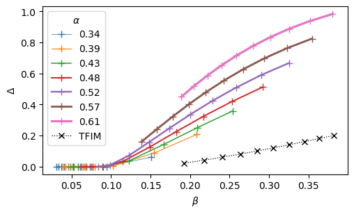
FIG. 2: Decay coefficient of the projection onto $\mathcal{L}$, $\beta$, vs. the gap $\Delta$ for different values of $J_{\text{ZZ}}$. Results are relative to a single chain of $l=300$, where it was numerically checked that the gap had stabilized to its value in the thermodynamic limit. $J_{\text{ZZ}}\in[2,4]$ for $h_{\text{XYZ}}$ and $J_{\text{ZZ}}\in[0.8,0.98]$ for $h_{\text{TFIM}}$, always in equal intervals, with smaller gaps corresponding to higher $J_{\text{ZZ}}$.

Discussion - We have obtained a simple hardware graph of maximum degree $d=3$ and 2-local interactions that is sufficient to encode any arbitrary Ising problem. By building the architecture from a decomposition of the original problem, a dual interpretation of the resulting graph is achieved: one in terms of consistent triangular cells and one in terms of chains of logical variables. The full architecture, incorporating local fields, requires $n=N(N-2)$ physical qubits and $c=N(3N-5)/2$ couplers, out of which $c_{\text{FM}}=N(N-2)$ will anneal to a strong ferromagnetic coupling. The sparsity of the graph also implies less crosstalk to keep under control, an important scalability feature. Achieving strong couplings without compromising coherence is a challenging task, but one that needs to be tackled nonetheless for any embedding strategy that enables scalability. In the particular case of superconducting technology, already standard couplers naturally provide a much larger ferromagnetic range than the antiferromagnetic one [4]. We have contributed to this scalability challenge from the algorithmic side by proposing alternative driver Hamiltonians that enhance the baseline success probability of the anneal by directing the search towards the logical subspace, mitigating the need for strong penalties. Some of these Hamiltonians can be readily implemented with current devices.

The triangle architecture discussed here is minimal: a graph of degree $d=3$ is the smallest to hold NP-complete problems [27]. As a consequence, a faulty element will truncate the maximum embedding size sharply depending on where the fault is located. Thus, this architecture has no tolerance to low fabrication yield, which limits its large-scale implementation as of today. In the particular case of superconducting quantum technologies (specifically for flux qubits) robust fabrication processes are still in their development phase, but yield should stop being an issue once the technology is mature.

All in all, the proposed scheme has several advantages: the embedding of the problem does not require any additional computation, the sparsity of the graph aids noise and crosstalk minimization and the interactions required are within the most employed model in current quantum annealing devices. In addition, the repetition code present in this architecture allows to spatially spread the information, making the computation more robust to some external error sources. Finally, the structure of the logical space allows to devise relatively simple driver Hamiltonians that mitigate the strength of the constraint terms.

Acknowledgments - We thank Ramiro Sagastizabal, Matthias Werner, Arnau Riera and Josep Bosch for valuable discussions. This work was supported by European Commission EIC-Transition project RoCCQeT (GA 101112839), the Agencia de Gestió d’Ajuts Universitaris i de Recerca through the DI grant (No. DI74) and the Spanish Ministry of Science and Innovation through the DI grant (No. DIN2020-011168).

References

- Kadowaki and Nishimori [1998] T. Kadowaki and H. Nishimori, Quantum annealing in the transverse Ising model, Physical Review E 58, 5355 (1998).
- Farhi et al. [2000] E. Farhi, J. Goldstone, S. Gutmann, and M. Sipser, Quantum Computation by Adiabatic Evolution, (2000), arXiv:quant-ph/0001106.
- Albash and Lidar [2018] T. Albash and D. A. Lidar, Adiabatic quantum computation, Rev. Mod. Phys. 90, 64 (2018).
- Weber et al. [2017] S. J. Weber, G. O. Samach, D. Hover, S. Gustavsson, D. K. Kim, A. Melville, D. Rosenberg, A. P. Sears, F. Yan, J. L. Yoder, W. D. Oliver, and A. J. Kerman, Coherent coupled qubits for quantum annealing, Physical Review Applied 8, 014004 (2017).
- Krantz et al. [2019] P. Krantz, M. Kjaergaard, F. Yan, T. P. Orlando, S. Gustavsson, and W. D. Oliver, A Quantum Engineer’s Guide to Superconducting Qubits, Applied Physics Reviews 6, 021318 (2019), arXiv: 1904.06560.
- Pohl et al. [2010] T. Pohl, E. Demler, and M. D. Lukin, Dynamical Crystallization in the Dipole Blockade of Ultracold Atoms, Physical Review Letters 104, 043002 (2010).
- de Léséleuc et al. [2018] S. de Léséleuc, S. Weber, V. Lienhard, D. Barredo, H. P. Büchler, T. Lahaye, and A. Browaeys, Accurate Mapping of Multilevel Rydberg Atoms on Interacting Spin-$1/2$ Particles for the Quantum Simulation of Ising Models, Physical Review Letters 120, 113602 (2018).
- Kaminsky et al. [2004] W. M. Kaminsky, S. Lloyd, and T. P. Orlando, Scalable Superconducting Architecture for Adiabatic Quantum Computation, (2004), arXiv:0403090.
- Choi [2008] V. Choi, Minor-embedding in adiabatic quantum computation: I. The parameter setting problem, Quantum Information Processing 7, 193 (2008).
- Choi [2011] V. Choi, Minor-embedding in adiabatic quantum computation: II. Minor-universal graph design, Quantum Information Processing 10, 343 (2011).
- Lechner et al. [2015] W. Lechner, P. Hauke, and P. Zoller, A quantum annealing architecture with all-to-all connectivity from local interactions, Science Advances 1, e1500838 (2015).
- Puri et al. [2017] S. Puri, C. K. Andersen, A. L. Grimsmo, and A. Blais, Quantum annealing with all-to-all connected nonlinear oscillators, Nature Communications 8, 15785 (2017).
- Mozgunov [2023] E. Mozgunov, Precision of quantum simulation of all-to-all coupling in a local architecture, (2023), arXiv:2302.02458.
- Fujii et al. [2022] T. Fujii, K. Komuro, Y. Okudaira, R. Narita, and M. Sawada, Energy landscape transformation of Ising problem with invariant eigenvalues for quantum annealing, (2022), arXiv:2202.05927.
- Fujii et al. [2023] T. Fujii, K. Komuro, Y. Okudaira, and M. Sawada, Eigenvalue-Invariant Transformation of Ising Problem for Anti-Crossing Mitigation in Quantum Annealing, Journal of the Physical Society of Japan 92, 044001 (2023).
- Venturelli et al. [2015] D. Venturelli, S. Mandrà, S. Knysh, B. O’Gorman, R. Biswas, and V. Smelyanskiy, Quantum Optimization of Fully Connected Spin Glasses, Physical Review X 5, 031040 (2015).
- Lanthaler and Lechner [2021] M. Lanthaler and W. Lechner, Minimal constraints in the parity formulation of optimization problems, New Journal of Physics 23, 083039 (2021).
- Albash et al. [2016] T. Albash, W. Vinci, and D. A. Lidar, Simulated-quantum-annealing comparison between all-to-all connectivity schemes, Physical Review A 94, 022327 (2016).
- Note [1] In the sense of restricting the evolution to the feasible space.
- Hen and Spedalieri [2016] I. Hen and F. M. Spedalieri, Quantum Annealing for Constrained Optimization, Physical Review Applied 5, 034007 (2016).
- Hen and Sarandy [2016] I. Hen and M. S. Sarandy, Driver Hamiltonians for constrained optimization in quantum annealing, Physical Review A 93, 062312 (2016).
-
Note [2]
Exemplary Hamiltonians of this type can be extracted from a circuit that builds a GHZ state. One such Hamiltonian is:
where corresponds to the -th chain of the chain set , all of which are of length . The ground and first excited states of Eq. (16) correspond to the even and odd GHZ states.(16) - Mbeng et al. [2020] G. B. Mbeng, A. Russomanno, and G. E. Santoro, The quantum Ising chain for beginners, Tech. Rep. arXiv:2009.09208 (arXiv, 2020) arXiv:2009.09208 [cond-mat, physics:quant-ph] type: article.
- Pfeuty [1970] P. Pfeuty, The one-dimensional Ising model with a transverse field, Annals of Physics 57, 79 (1970).
- Baxter [1990] R. J. Baxter, Exactly solved models in statistical mechanics, 2nd ed. (Acad. Press, London, 1990).
- Shi et al. [2020] Q.-Q. Shi, S.-H. Li, and H.-Q. Zhou, Duality and ground-state phase diagram for the quantum XYZ model with arbitrary spin in one spatial dimension, Journal of Physics A: Mathematical and Theoretical 53, 155301 (2020).
- Barahona [1982] F. Barahona, On the computational complexity of Ising spin glass models, Journal of Physics A: Mathematical and General 15, 3241 (1982).