Scalar Field Dark Matter Around Charged Black Holes

Abstract

In this paper, we investigate the behavior of a massive scalar field dark matter scenarios in the large mass limit around a central Reissner-Nordström black hole. This study is motivated by observations from the Event Horizon Telescope collaboration, which does not exclude the possibility of the existence of such black holes. Through these inquiries, we uncover that the electric charge may significantly impact the scalar field profile and the density profile in the vecinty of the black hole. For the maximum electric charge allowed by the constraints of the Event Horizon Telescope, the maximum accretion rate decreases by $\thicksim$ 50 % compared to the Schwarszchild case for marginally bound orbits. The maximum accretion rate of the massive scalar field is approximately $\dot{M}_{\text{SFDM}}\thicksim 10^{-8}M_{\odot}\;\text{yr}^{-1}$, which is significantly lower than the typical baryonic accretion rate commonly found in the literature. This implies that the scalar cloud located at the center of galaxies may have survived untill present times.

I Introduction

There is robust evidence suggesting the presence of an invisible component in the observable Universe, known as dark matter (DM) Spergel et al. (2003); Ade et al. (2016); Aghanim et al. (2020); Tegmark et al. (2004); Anderson et al. (2014); Alam et al. (2017). The most accepted and successful model to date is cold dark matter (CDM), which describes DM as a non-relativistic perfect fluid. However, CDM faces challenges when trying to explain observations at galactic and subgalactic scales. For instance, $N$-body simulations for CDM indicate a pronounced increase in the density profile (spike) as we approach the centers of galaxies. This is referred to as the universal or Navarro-Frenk-White (NFW) profile $\rho_{\text{NFW}}$ Navarro et al. (1996). In contrast, observations suggest constant density profiles forming a core toward the center Moore (1994); de Blok (2010). This aspect is more evident in dwarf spheroidal and low-mass spiral galaxies Oh et al. (2011), as is the well-known discrepancy of 2-3 orders of magnitude in the number of satellite galaxies between observations and theoretical predictions Moore et al. (1999); Bullock et al. (2000), or the famous problem known as “too big to fail” Boylan-Kolchin et al. (2011); Garrison-Kimmel et al. (2014). However, some research suggests that taking into account the baryonic feedback effects Del Popolo and Le Delliou (2017); Dutton et al. (2019, 2020) or even the supernova feedback Sommer-Larsen and Vedel (1999) could help alleviate these tensions. With all of the aforementioned, the idea of exploring new concepts emerges. Some researchers propose modifying gravity in the low-acceleration regime Milgrom (1983) or suggesting alternative models for DM. In this work, we will focus on the latter proposal.

Scalar field dark matter (SFDM) is a well-grounded candidate that arises as an extension of the standard model of particle physics and proposes DM is composed of ultralight bosonic particles with zero spin, spanning a mass range from 10^-22 eV to 1 eV. This model has gained prominence recently due to its potential to address some of these issues Hu et al. (2000); Hui et al. (2017); Ferreira (2021), as it possesses de Broglie wavelength on the order $\thicksim$ kpc. Within the SFDM model, there are various subcategories, including examples such as fuzzy dark matter (FDM) Hu et al. (2000); Hui et al. (2017); Sin (1994); Ji and Sin (1994); Seidel and Suen (1990); Matos and Guzman (2000); Hui et al. (2019); Dave and Goswami (2023), where the particle is typically associated with a mass on the order $\thicksim$ 10^-22 eV, self-interacting scalar field dark matter (SIDM) Goodman (2000); Peebles (2000); Arbey et al. (2003); Boehmer and Harko (2007); Lee and Lim (2010); Harko (2011); Rindler-Daller and Shapiro (2012); Suárez et al. (2014); Ureña López (2019), involving coupling between particles, the well-known Axions Peccei and Quinn (1977); Wilczek (1978); Weinberg (1978), originally proposed to address the CP symmetry violation problem, and also Axion-Like-Particles (ALPs) proposed in other theories Marsh (2016). The main distinction among the aforementioned models lies in the mass range or the associated coupling of these particles Kobayashi et al. (2017); Abel et al. (2017); Brito et al. (2017a, b).

A fascinating aspect of SFDM models is that the stationary solutions of these classical bosonic fields, known as solitons, could be present in galactic centers, providing a plausible explanation for the observed constant density profiles Arbey et al. (2001); Schive et al. (2014); Marsh and Pop (2015); Schwabe et al. (2016); Mocz et al. (2017); Levkov et al. (2018); Chavanis (2011); Chavanis and Delfini (2011). These solitonic cores would form structures ranging from 1 kpc to 20 kpc. In the case of FDM, it would be attributed to quantum pressure, arising from the uncertainty principle, while for SIDM, it would be due to self-interaction (repulsive). However, these would not be the only mechanisms for the formation of gravitationally bound structures at the galactic level. In fact, galactic halos are expected to be in equilibrium due to virialized motion Schneider (2015). Additionally, these models could also explain the observed vortices in galaxies Rindler-Daller and Shapiro (2012); Peebles (1969); Kain and Ling (2010). Although current measurements Kobayashi et al. (2017); Iršič et al. (2017); Rogers and Peiris (2021); Bar et al. (2022) suggest a minimum mass limit of around $m\gtrsim 10^{-22}$ eV for the FDM model.

The vast majority of galaxies in the Universe host supermassive black holes (SMBHs) at their centers Kormendy and Richstone (1995); Ferrarese and Ford (2005); Narayan (2005). The prevailing notion is that these black holes (BHs) are surrounded by a solitonic core, which, in turn, is enveloped by a halo of DM. Some researches have suggested the possibility that these BHs possess a non-zero value of net electric charge Zakharov (2014); Juraeva et al. (2021). This idea has gained recent support from the Event Horizon Telescope (EHT) collaboration Kocherlakota et al. (2021); Akiyama et al. (2022), which first captured the shadow image of M87^⋆ Kocherlakota et al. (2021) and later did the same for Sagittarius A^⋆ (SgrA^⋆) Akiyama et al. (2022); Vagnozzi et al. (2022). These studies indicate that the charge-mass ratio $q=Q/M$ for M87^⋆ falls within the range of $q\in[0,0.9]$ Kocherlakota et al. (2021), while for SgrA^⋆, it is $q\in[0,0.84]$ Akiyama et al. (2022). Nevertheless, it is widely disseminated in the community that BHs are electrically neutral since the surrounding plasma would rapidly discharge them. It is important to note that this article will not delve into the origin of electric charge or the timescales during which a BH might remain electrically charged. Therefore, we strictly adhere to the observational constraints from EHT.

The nature of DM remains unknown. However, with the first detection of gravitational waves (GWs) Abbott et al. (2016), another research frontier opened up in this field. It is possible that within the signal of GWs, relevant information about the medium in which BHs are immersed may be inferred, making it a feasible probing option to explore the nature of DM Eda et al. (2013); Lacroix and Silk (2013); Kavanagh et al. (2020); Gómez et al. (2016); Bar et al. (2019); Saurabh and Jusufi (2021); Boudon et al. (2023); Chakrabarti et al. (2022). Nevertheless, the impact that DM has on the GW signal depends on the its properties, such as the density peofile. Therefore, it is of vital importance to carry out accurate and self-consistent modeling of DM around black holes. For instance, density profiles could differ depending on whether it is CDM Sadeghian et al. (2013) or SFDM Barranco et al. (2011); Clough et al. (2019); Bamber et al. (2021); Hui et al. (2019); Aguilar-Nieto et al. (2023); Brax et al. (2020); Vicente and Cardoso (2022); Cardoso et al. (2022), and to this day, the discussion about the existence of “scalar hair” continues Jacobson (1999); Hui et al. (2019); Brihaye and Hartmann (2022).

Currently, there exists an extensive literature on the study of scalar fields in Schwarzschild space-time (see, for example, Unruh (1976); Detweiler (1980); Hui et al. (2019)); however, only a small handful of studies delve into the realm of “non-standard metrics” (see e.g. Benone et al. (2014)). It is precisely within this context that our research is aimed.

In this study, we specifically focus on investigating the behavior of a non-interacting massive scalar field DM in the large-mass limit ($m\gg 10^{-22}$ eV) around a Reissner-Nordström (RN) BH Reissner (1916). We establish a direct connection between these results and our previous research Ravanal et al. (2023), following a similar path to that taken by Brax et al. (2020). We uncover that the influence of the electric charge $Q$ becomes relevant in regions close to marginally bound orbits. Considering this argument Ravanal et al. (2023); Sadeghian et al. (2013), a maximum accretion rate of the scalar field DM of $\dot{M}_{\text{SFDM}}\thicksim 10^{-8}M_{\odot}\;\text{yr}^{-1}$ was obtained, with a decrease of approximately 50 % when $Q$ becomes significant compared to the uncharged case. Within the constraints allowed by the EHT, the accretion in the non-interacting case, which corresponds to a free-falling, is higher compared to the SIDM case Feng et al. (2022); Ravanal et al. (2023), since in the latter, the repulsive self-interaction slows down the DM fall. This features determines the lifetime and the mass of the extended cloud and have critical consequences for the observed shadow radius Gómez and Valageas (2024). Furthermore, a scalar field profile $\phi\propto r^{-3/4}$ was observed, which coincides with the same power law as other studies in the same regime of interest Hui et al. (2019); Clough et al. (2019); Bucciotti and Trincherini (2023). Finally, a change in the power-law exponents $\rho\propto r^{-3/2}$ and $\rho\propto r^{-1}$ for the density profile in the non-interactive and interactive cases, respectively, was observed. This change originates evidently from the nature of the studied fields. These exponents fall within the usual range considered in various power-law models for dark matter density profiles Ferreira (2021).

This paper is structured as follows. In section II, we describe the theoretical framework, including the DM model, conditions of steady-state accretion, and the resulting scalar field profile. In section III, we establish a direct connection with our previous work Ravanal et al. (2023), and compare our main findings with other works. Finally, in section IV, we provide a detailed discussion of our results and their potential implications.

II Dark Matter Scalar Field

The relativistic action of a real scalar-field (SF) minimally coupled to gravity is given by

$$S=S_{\text{EH}}+S_{\phi}=\int d^{4}x\sqrt{-g}\left[\frac{\mathcal{R}}{16\pi}-\frac{1}{2}g^{\mu\nu}\partial_{\mu}\phi\partial_{\nu}\phi-V(\phi)\right].$$ (1)

Here $S_{\text{EH}}$ represents the Einstein-Hilbert action, $S_{\phi}$ corresponds to the action for a single real SF $\phi$, $g_{\mu\nu}$ represents the metric, $\mathcal{R}$ denotes the Ricci scalar, $g$ stands for the determinant of the metric $g_{\mu\nu}$, and $V(\phi)$ is the SF potential. In this study, we adhere to metric signature conventions of $(-,+,+,+)$ and use units where $4\pi\epsilon_{0}=G=c=\hbar=1$.

The equation of motion for the SF, derived from Eq. (1), takes the following form

$$\frac{\delta S_{\phi}}{\delta\phi}=0\;\;\;\Longrightarrow\;\;\;\Box\phi-\frac{dV}{d\phi}=0,$$ (2)

where the covariant d’Alembertian $\Box$ is defined as $\Box=\nabla^{\mu}\nabla_{\mu}=g^{\mu\nu}\nabla_{\mu}\nabla_{\nu}$. For the potential $V(\phi)=m^{2}\phi^{2}/2$, we derive the well-known Klein-Gordon equation $(\Box-m^{2})\phi=0$. Additionally, starting from Eq. (1), we can calculate the energy-momentum tensor for the SF, expressed as $T^{\mu\nu}=(2/\sqrt{-g})\;\delta S_{\phi}/\delta g_{\mu\nu}$.

In this article, we consider the large-mass limit Hui et al. (2019); Brax et al. (2019) given by

$$m\gg 6.7\times 10^{-19}\;\left(\frac{M}{10^{8}M_{\odot}}\right)^{-1}{\rm eV},$$ (3)

where the characteristic length scale of the system surpasses the Compton wavelength $\lambda_{C}\thicksim 1/m\ll r_{\text{h}}$. Here $r_{\text{h}}$ is the radius of the event horizon. In this regime, we can neglect the quantum pressure $\Phi_{Q}$. This pressure stems from Heisenberg’s uncertainty principle $\Delta x\Delta p\thicksim 1$ and is insignificant at galactic and subgalactic scales within our regime. Consequently, the SFDM cloud is governed by self-gravity at these scales, reaching a virial equilibrium state where the kinetic energy of the particles equals the gravitational potential energy.

Before deriving the master equations, we outline the primary physical assumptions made in this work, aiming to enhance clarity:

• Radial accretion flows on static spherically symmetric BHs.

• large scalar mass limit where the Compton wavelength $1/m$ is smaller than the BH size.

• Test-fluid approximation where the backreaction of the scalar cloud to the spacetime metric is neglected.

II.1 Spherically symmetric space-times

For a spherically symmetric spacetime the metric takes the form

$$ds^{2}=-f(r)dt^{2}+g(r)dr^{2}+r^{2}d\vec{\Omega}^{2},$$ (4)

where the metric functions $f(r)$ and $g(r)$ for a RN metric are given by

$$f(r)=\frac{1}{g(r)}=1-\frac{2M}{r}+\frac{Q^{2}}{r^{2}},$$ (5)

with the corresponding horizons

$$r_{\pm}=M\pm\sqrt{M^{2}-Q^{2}}.$$ (6)

$M$ represents the mass of the BH, and $Q$ denotes the electric charge. The BH metric exhibits two event horizons: $r_{+}$ corresponds to the outer horizon (of primary interest in this study), while $r_{-}$ corresponds to the Cauchy horizon. The Schwarzschild solution is readily obtained when $Q=0$, and the scenario $Q=M$ represents the extremal case. The metric functions can be easily expressed as a function of dimensionless quantities through the following variable transformation

$$x=\frac{r}{M}\geq 1,\;\text{and}\;\;\;q=\frac{Q}{M},$$ (7)

where $x$ denotes the new radial coordinate, and $q$ represents the charge-to-mass ratio. Utilizing these variables, we can describe the horizons in the following manner

$$x_{\pm}=1\pm\sqrt{1-q^{2}}:\;\;\;0\leq q\leq 1.$$ (8)

It is important to note that for the sake of completeness, there are two other possible cases in Eq. (8). The first one is when $q>1$, which describes a naked singularity without an event horizon, and the second one is when $q^{2}$ is negative. However, in this work, we will not consider these two cases, as we will focus solely on the constraints imposed by the EHT Kocherlakota et al. (2021); Akiyama et al. (2021, 2022); Vagnozzi et al. (2022).

In this scenario, we can divide the physical regions of interest around the BH into three zones as follows:

• region near the BH ($r_{+}<r<r_{\text{NL}}$): This region extends from the horizon $r_{+}$ to a non-linear radius $r_{\text{NL}}$. It is denoted as the strong-gravity regime, where the metric functions in the vicinity of the BH are defined by Eq. (5).

• intermediate region ($r_{\text{NL}}\ll r\ll r_{\text{sg}}$): This region is defined by the Newtonian limit ($\Phi=-M/r\ll 1$), in which the line element turns out to be: $ds^{2}=-(1+2\Phi)dt^{2}+(1-2\Phi)\vec{dr}\cdot\vec{dr}$. This case corresponds to the weak gravity regime, where the black hole’s influence is still noticeable.

• region far from the BH ($r\gg r_{\text{sg}}$): This region extends well beyond the transition radius $r_{\text{sg}}$ and is primarily controlled by the self-gravity of the DM cloud, where the gravitational potential $\Phi$ is governed by the scalar field’s Poisson equation

  $$\nabla^{2}\Phi=4\pi\rho_{\phi},$$ (9)

  where $\rho_{\phi}$ stands for the energy density of the SF.

II.2 Free Scalar Field

We star by examining the profile of the free SF flow around the RN-BH.

II.2.1 Equations of motion

The relativistic action of the SF (1) is expressed in terms of the metric (4)

$$S_{\phi}=\int dtdrd\theta d\varphi\sqrt{fg}r^{2}\sin\theta\left[\frac{1}{2f}\left(\frac{\partial\phi}{\partial t}\right)^{2}-\frac{1}{2g}\left(\frac{\partial\phi}{\partial r}\right)^{2}\right.\\ \left.-\frac{1}{2r^{2}}\left(\frac{\partial\phi}{\partial\theta}\right)^{2}-\frac{1}{2r^{2}\sin^{2}\theta}\left(\frac{\partial\phi}{\partial\varphi}\right)^{2}-V(\phi)\right].$$ (10)

In the non-relativistic limit, the real SF $\phi$, whose frequency oscillations are dominated by the mass term $m$, can be expressed in terms of a complex SF $\psi$, as described below

$$\phi=\frac{1}{\sqrt{2m}}\left(e^{-imt}\psi+e^{imt}\psi^{*}\right).$$ (11)

We can observe that $\phi$ exhibits a global symmetry of the $U(1)$ group, signifying its invariance under continuous phase rotations $\xi$. In the non-relativistic limit, the conservation of the Noether current implies a particle number conservation, or mass conservation, and the transformation is defined as follows

$$\left.\begin{array}[]{c}\psi\longrightarrow\psi e^{i\xi}\\ \psi^{*}\longrightarrow\psi e^{-i\xi}\end{array}\right\}\Longrightarrow\phi\longrightarrow\phi.$$ (12)

In this low-energy regime ($m$ is of the order of the rest mass, i.e., the momentum is small compared to this one), and where field oscillations vary slowly $\dot{\psi}\ll m\psi$, where the overdot denotes a time derivative, we can express the action of the complex scalar field $\psi$ as follows

$$S_{\psi}=\int dtdrd\theta d\varphi\sqrt{fg}r^{2}\sin\theta\left[\frac{1}{2f}(i\dot{\psi}\psi^{*}-i\psi\dot{\psi}^{*}\right.\\ +m\psi\psi^{*})-\frac{1}{2mg}\frac{\partial\psi}{\partial r}\frac{\partial\psi^{*}}{\partial r}-\\ \frac{1}{2mr^{2}}\frac{\partial\psi}{\partial\theta}\frac{\partial\psi^{*}}{\partial\theta}\left.-\frac{1}{2mr^{2}\sin^{2}\theta}\frac{\partial\psi}{\partial\varphi}\frac{\partial\psi^{*}}{\partial\varphi}-\frac{m}{2}\psi\psi^{*}\right].$$ (13)

Usually, rapid oscillations $e^{\pm 2imt}$ are discarded, as their average is approximately zero under the previously described assumptions. Finally, we can derive the Euler-Lagrange equations for the field $\psi$

$$i\dot{\psi}=-\frac{f}{2m}\left[\frac{1}{\sqrt{fg}}\vec{\nabla}_{r}\cdot\left(\sqrt{\frac{f}{g}}\vec{\nabla}_{r}\psi\right)+\nabla^{2}_{\theta,\varphi}\psi\right]+m\frac{f-1}{2}\psi.$$ (14)

Here, $\vec{\nabla}_{r}$ and $\vec{\nabla}_{\theta,\varphi}$ represent the radial and angular components of the nabla operator, respectively. On the other hand, we can recover the non-relativistic version for $\psi$ at large distances, as the metric functions are recovered in the weak-field limit (intermediate region in section II.1)

$$r\gg r_{\text{h}}\;\;:\;i\dot{\psi}=-\frac{\vec{\nabla}^{2}\psi}{2m}+m\Phi\psi.$$ (15)

We can observe that the above expression is a Schrödinger-type equation. It is possible to approach this problem within the fluid description using the Mandelung transformations Madelung (1927)

$$\psi=\sqrt{\frac{\rho}{m}}e^{is}\;\;\;,\;\;\;\rho=m|\psi|^{2},$$ (16)

where $\sqrt{\rho/m}$ represents the amplitude and $s$ is a phase, $\rho$ serves as the SF matter density, and the velocity field is defined as follows

$$\vec{v}=\frac{\vec{\nabla}s}{m},$$ (17)

in this description, the flow is defined as irrotational. Furthermore, with the previously mentioned definitions, we can express the real scalar field profile as follows

$$\phi=\frac{\sqrt{2\rho}}{m}\cos(mt-s).$$ (18)

It is possible to express the action $S_{\psi}$ in terms of the new quantities $\rho$ and $s$ through the Madelung transformations. The new action now reads:

$$S_{\rho,s}=\int dtdrd\theta d\varphi\sqrt{fg}r^{2}\sin\theta\biggl{\{}-\frac{\rho\dot{s}}{mf}-\frac{1}{2m^{2}g}\left[\frac{1}{4\rho}\left(\frac{\partial\rho}{\partial r}\right)^{2}\!\!+\rho\left(\frac{\partial s}{\partial r}\right)^{2}\right]-\frac{1}{2m^{2}r^{2}}\left[\frac{1}{4\rho}\left(\frac{\partial\rho}{\partial\theta}\right)^{2}\right.\left.+\rho\left(\frac{\partial s}{\partial\theta}\right)^{2}\right]$$

$$-\frac{1}{2m^{2}r^{2}\sin^{2}\theta}\left[\frac{1}{4\rho}\left(\frac{\partial\rho}{\partial\varphi}\right)^{2}\!\!+\rho\left(\frac{\partial s}{\partial\varphi}\right)^{2}\right]+\frac{\rho}{2f}-\frac{\rho}{2}\biggl{\}}.$$ (19)

As mentioned earlier, in the large-mass limit, neglecting spatial gradients $|\vec{\nabla}\rho|\ll m\rho$ is equivalent. However, since the phase $s$ is of the order of $m$, the action is consequently reduced to the following form

$$S_{\rho,s}=\int dtdrd\theta d\varphi\sqrt{fg}r^{2}\sin\theta\Biggl{[}-\frac{\rho\dot{s}}{mf}-\frac{\rho}{2m^{2}g}\left(\frac{\partial s}{\partial r}\right)^{\!\!2}\\ -\frac{\rho}{2m^{2}r^{2}}\left(\frac{\partial s}{\partial\theta}\right)^{\!2}-\frac{\rho}{2m^{2}r^{2}\sin^{2}\theta}\left(\frac{\partial s}{\partial\varphi}\right)^{\!\!2}\\ +\frac{\rho(1-f)}{2f}\Biggr{]}.$$ (20)

We can obtain the equations of motion from action (20), that is, $\delta S/\delta s=0$, resulting in

$$\dot{\rho}+f\left[\frac{1}{\sqrt{fg}}\vec{\nabla}_{r}\cdot\left(\sqrt{\frac{f}{g}}\rho\frac{\vec{\nabla}_{r}s}{m}\right)+\vec{\nabla}_{\theta,\varphi}\cdot\left(\frac{\rho}{m}\vec{\nabla}_{\theta,\varphi}s\right)\right]=0.$$ (21)

The same applies to $\delta S/\delta\rho=0$:

$$\frac{\dot{s}}{m}+\frac{f}{2}\left[\frac{1}{g}\frac{(\vec{\nabla}_{r}s)^{2}}{m^{2}}+\frac{(\nabla_{\theta,\varphi}s)^{2}}{m^{2}}\right]=\frac{1-f}{2}.$$ (22)

By taking the gradient of Eq. (22) and using the definition of the velocity field (17), in Eqs. (21) and (22) we have

$$\dot{\rho}+f\left[\frac{1}{\sqrt{fg}}\vec{\nabla}_{r}\cdot\left(\sqrt{\frac{f}{g}}\rho v_{r}\right)+\vec{\nabla}_{\theta,\varphi}\cdot\left(\rho v_{\theta,\varphi}\right)\right]=0,$$ (23)

$$\dot{\vec{v}}+\vec{\nabla}\left[\frac{f}{2}\left(\frac{v^{2}_{r}}{g}+v^{2}_{\theta,\varphi}\right)\right]=-\frac{\vec{\nabla}f}{2}.$$ (24)

For very large distances ($r\gg r_{\text{h}}$), the metric functions are recovered in the weak-field limit, and by using vector identities, we obtain

$$\dot{\rho}+\vec{\nabla}\cdot(\rho\vec{v}) =0,$$ (25)

$$\dot{\vec{v}}+(\vec{v}\cdot\vec{\nabla})\vec{v} =-\vec{\nabla}\Phi.$$ (26)

Eqs. (25) and (26) represent the continuity and Euler equations, respectively. Both equations correspond to the classical limit that governs fluid dynamics. It is important to mention that Euler’s equation (26), which lacks a pressure term, corresponds to the free motion of particles under the influence of a gravitational potential $\Phi$. It is important to mention that, starting from Eq (15) and using the Madelung transformations Eqs. (16) and (17), when separating the real and imaginary parts, we obtain the same equations (continuity and Euler) in the non-relativistic limit. We neglect the quantum pressure $\Phi_{Q}=-(\nabla^{2}/2m^{2})(\sqrt{\rho}/\sqrt{\rho})$, as we are in the large-mass limit, where the momentum are considerably smaller compared to the rest mass.

II.2.2 Steady state

We can find stationary solutions to Eqs. (23) and (24), and restricting to spherical symmetry (4), we obtain the following solution to the continuity equation (23)

$$\sqrt{\frac{f}{g}}r^{2}\rho v_{r}=F,$$ (27)

where $F<0$ is defined as an inward flux per unit solid angle; in other words, DM falls into the BH steadily.

From the Euler equation (24), we obtain

$$v_{r}=\pm\sqrt{\frac{g(1-f)}{f}}\;\;\;,\;\;\;mv_{r}=\frac{\partial s}{\partial r}.$$ (28)

In our case, we choose the negative sign solution, as DM particles fall radially towards the BH. Near the horizon, we observe a divergence when $f\to 0$, which is caused by the use of non-regular coordinates. Furthermore, we can see that as the radius tends to infinity, the radial velocity tends to zero, which sets the boundary condition of the problem.

We can obtain the matter density of the SF from Eqs. (27) and (28). This expression is valid in the large-mass limit, where we observe that massive particles fall radially toward the BH, regardless of their mass. They start at rest from infinity and free-fall into the vicinity of the BH

$$\rho=-\frac{F}{r^{2}\sqrt{1-f}}.$$ (29)

When we approach the BH horizon, we notice that $f\to 0$. At this point, we observe that $\rho$ is finite and equals $-F/r_{\text{h}}^{2}$. In contrast, when we are at very large distances, $f$ approaches unity, and consequently, $\rho\to 0$ because the quadratic term decreases faster than the metric function $f$.

II.2.3 Scalar field profile

It is possible to rewrite the SF profile, considering the stationary solutions imposed in the previous section. This is achieved by substituting Eq. (29) into Eq. (18), and the phase $s$ is obtained from the expressions in (28). This gives

$$\phi=\frac{1}{2mM}\sqrt{\frac{-8F}{x^{2}\sqrt{1-f}}}\cos(mt-s).$$ (30)

This expression represents an harmonic ingoing wave propagating towards the BH, as shown in Fig. (1). The SF profile exhibits then oscillatory behavior. As we approach the BH, its amplitude increases or in the opposite case, it decreases, pimarily due to the denominator within the square root. We can observe that the effects of $q$ become significant in the vicinity of the BH; indeed, as $q$ increases, an increase in amplitude is observed, mainly because a BH with significant charge has a smaller event horizon compared to the uncharged case. To further clarify this idea, it is convenient to remove the temporal dependence of the SF profile (30), as shown in Fig. (2). These curves essentially represent the amplitude of the SF profile. Once more, it is observed that as the charge $q$ increases, the amplitude near the black hole also increases. At this point, we bring up Jacobson’s results Jacobson (1999), who obtained a non-vanishing solution for a massless scalar field by imposing the boundary condition of a non-zero time derivative far away from the BH. He obtained SF profile that behaves as $\phi\propto r^{-1}$ for large radii. In our case of large-mass limit framed on DM scenarios, the decay behaves differently, specifically as $\phi\propto x^{-3/4}$ for large radii.

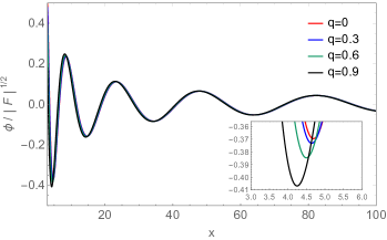
Figure 1: Normalized scalar field profile $\phi(x)/|F|^{1/2}$ as a function of the radial coordinate $x$, for different values of the charge-mass ratio $q$, as given by Eq. (30). The zoomed-in window pertains to the region between the photon sphere $x_{\text{ph}}$ and the innermost stable circular orbit $x_{\text{isco}}$, which uncovers the effect of the BH charge on the scalar profile.

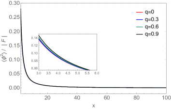
Figure 2: Normalized time-averaging of the square scalar field profile $\langle\phi^{2}\rangle/|F|$ as a function of the radial coordinate $x$, for different values of the charge-mass ratio $q$, as derived from Eq. (30). The zoomed-in window pertains to the region between the photon sphere $x_{\text{ph}}$ and the innermost stable circular orbit $x_{\text{isco}}$.

II.2.4 Density profile

From relativistic action (1), it is possible to obtain the energy-momentum tensor $T_{\alpha\beta}=\partial_{\alpha}\phi\partial_{\beta}\phi+g_{\alpha\beta}\mathcal{L}_{\phi}$, where $\mathcal{L}_{\phi}$ is the lagrangian of the SF. Under the symmetry of our problem (4), we can express the energy density of the SF $\rho_{\phi}$, which is associated with the time-time component of the energy-momentum tensor

$$\rho_{\phi}\equiv-T^{t}_{t}=\frac{1}{2f}\left(\frac{\partial\phi}{\partial t}\right)^{2}+\frac{1}{2g}\left(\frac{\partial\phi}{\partial r}\right)^{2}+V(\phi).$$ (31)

Replacing the SF profile (18) in the previous equation and considering the large mass limit, we obtain

$$\rho_{\phi}=\rho\left[\frac{(2-f)}{f}\sin^{2}(mt-s)+\cos^{2}(mt-s)\right].$$ (32)

Finally, expressing it in terms of the flux $F$ and averaging over the rapid oscillations with a period of $2\pi/m$, we obtain:

$$\langle\rho_{\phi}\rangle=-\frac{4F}{(2M)^{2}x^{2}f\sqrt{1-f}}.$$ (33)

It is important to note that $q$ is constrained between 0 and 0.9 according to the EHT Kocherlakota et al. (2021); Akiyama et al. (2021, 2022); Vagnozzi et al. (2022). With all of this in mind, we can study the behavior of the density profile of this massive SF around a RN-BH. The average energy density $\langle\rho_{\phi}\rangle$ diverges as we approach the horizon. This divergence is caused by the term $1/f$, as $f\to 0$, as a result of using non-regular coordinates. At large distances, we have $\langle\rho_{\phi}\rangle\propto x^{-3/2}$ and $|\;v\;|\propto x^{-1/2}$. This can be interpreted as a free particle falling from infinity with a velocity $\propto r^{-1/2}$ due to the conservation of energy, similar to virialized DM halos $v_{r}^{2}\thicksim\Phi\thicksim M/r$.

To provide a clearer understanding of the behavior of the massive SF around an RN-BH, Fig. (3) displays the normalized energy density of the SF, referred to as $\langle\rho_{\phi}\rangle/|F/(2M)^{2}|$, for various values of $q$. It can be observed that at larger distances, the influence of $q$ becomes imperceptible. This fact arises, not surprisingly, because the term $(q/x)^{2}$ within the metric function rapidly diminishes with increasing distance. However, the zoomed-in window suggests that $q$ has an impact on the region located between the photon sphere $x_{\text{ph}}$ and the innermost stable circular orbit $x_{\text{isco}}$—a region where marginally bound orbits $x_{\text{mb}}$ are typically located, making it inevitable to fall into the RN-BH. As the charge is turned on, the density profile becomes less cuspy compared to the Schwarzschild case at small radii. At such distances, the profile no longer follows the simple scaling: $\rho\propto x^{-3/2}$. This is mainly because as $q$ increases, the horizon radius becomes smaller, reducing its effective cross-section for capturing DM particles. The region mentioned above is particularly of interest for current and upcoming BHs experiments in the strong field regime that could potentially reveal deviations from standard geometries, shedding light on “scalar hair” phenomena.

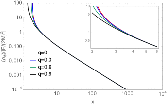
Figure 3: Normalized energy density of the scalar field $\langle\rho_{\phi}\rangle/|F/(2M)^{2}|$ as a function of the radial coordinate x, for different charge-mass ratios q, as given by Eq. (33). The abrupt density spike around the respective horizon is a result of employing nonregular coordinates at the horizon. The zoomed-in window pertains to the region between the radius horizon $x_{\text{h}}$ and the innermost stable circular orbit $x_{\text{isco}}$.

II.2.5 Accretion

We compute the mass accretion rate around a RN-BH. The mass accretion can be obtained from the continuity equation is associated with the component $\nu=t$ of the conservation equations $\nabla_{\mu}T^{\mu}_{\nu}=0$. For a steady state, the mass accretion rate is defined as the energy flow through a closed surface of a sphere, given by

$$\dot{M}(r)=\oint T^{r}_{t}\sqrt{-g}d\theta d\varphi,$$ (34)

where

$$T_{t}^{r}=\frac{1}{g}\frac{\partial\phi}{\partial r}\frac{\partial\phi}{\partial t}.$$ (35)

Using the SF profile (18) and considering the large-mass limit, we can calculate the mass accretion of DM

$$\dot{M}_{\text{SFDM}}=4\pi r^{2}\rho\sqrt{1-f},$$ (36)

We can observe that the above expression is regular at the horizon. Typically, $r_{\text{isco}}$ is identified as the region where the maximum accretion rate is experienced Shapiro and Teukolsky (1983); Gondolo and Silk (1999). However, other studies Sadeghian et al. (2013); Ravanal et al. (2023) suggest that accretion occurs in the region where marginally bound orbits ($r_{\text{mb}}\lesssim r\lesssim r_{\text{isco}}$) are located. Indeed, it is in this region where particle capture occurs. Hence, we shall restrict our analysis to such scales. To better visualize this situation, we show in Fig. (4) various orbits of interest. In particular, we assume that the maximum rate is attained at $r_{\text{mb}}$. Our previous study Ravanal et al. (2023), in the case of a self-interacting scalar field, supports this possibility by indicating that the maximum rate occurs on marginally bound orbits.

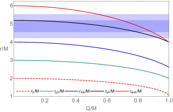
Figure 4: The image displays various orbits and regions of interest in the vicinity of a RN-BH. We can distinguish the horizon $r_{\text{h}}/M$ (dashed red line) Pugliese et al. (2011), the photon sphere $r_{\text{ph}}/M$ (Green line) Pugliese et al. (2011), the marginally bound radius $r_{\text{mb}}/M$ (blue line) Beheshti and Gasperin (2016), the shadow radius $r_{\text{sh}}/M$ of the RN-BH (black line) Vagnozzi et al. (2022), and the innermost stable circular orbit $r_{\text{isco}}/M$ (red line) Pugliese et al. (2011); Gómez and Rodríguez (2023). Additionally, the sky blue region $4.55\lesssim r_{\text{sh}}/M\lesssim 5.21$ corresponds to the $1\sigma$ constraint, while the light blue region $4.21\lesssim r_{\text{sh}}/M\lesssim 5.56$ corresponds to the $2\sigma$ constraint, set by Keck and VLTI telescopes, respectively Vagnozzi et al. (2022). The EHT provides the constraint $Q/M\in[0,0.9]$ Kocherlakota et al. (2021); Akiyama et al. (2021, 2022); Vagnozzi et al. (2022).

We observe a decrease of approximately 50% and 42% in the accretion rate for the maximum allowed charge $q=0.9$ at $r_{\text{mb}}$ and $r_{\text{isco}}$, respectively, compared to the uncharged case. To gain a sense of the order of magnitude of accretion in this scenario, let’s consider a Milky Way-like galaxy, which have a dark matter density $\rho_{\text{DM}}\thicksim 10^{6}M_{\odot}\;\text{pc}^{-3}$ Sadeghian et al. (2013). Evaluating the maximum accretion rate of scalar field dark matter gives $\dot{M}_{\text{SFDM}}\thicksim 10^{-8}M_{\odot}\;\text{yr}^{-1}$. This level of accretion is higher than that found by repulsive SIDM models, which is on the order of $\dot{M}_{\rm SIDM}\sim 10^{-10}M_{\odot}~{}{\rm yr}^{-1}$ Feng et al. (2022); Ravanal et al. (2023). This result makes sense, as the existence of repulsion between particles suggests that the number of particles falling into the BH should be lower. However, all these estimations are small compared to baryonic matter accretion, suggesting the possibility that gravitationally bound structures composed of DM remain present in the galaxy. In fact, these structures should have a critical mass that surpasses millions of solar masses to reach the Bondi-like pressure-regulated infall Gómez and Valageas (2024).

III Comparison with previous results

III.0.1 Self-interacting scalar field dark matter

We present a brief summary of our previous work Ravanal et al. (2023) and highlight how this new work connects with it. When a quartic self-interaction potential is included in Eq. (2), the nonlinear Klein-Gordon equation is obtained. In the large scalar-mass limit (3), this equation can be identified as a Duffing-type equation Kovacic and Brennan (2011), which describes a nonlinear harmonic oscillator, and its analytical solution can be expressed in terms of Jacobi elliptic functions Brax et al. (2020); Frasca (2011). It is important to note that at distances beyond the transition radius $r_{\text{sg}}$, we enter the domain where the self-gravity of the soliton turns out to be important. This arises from the hydrostatic equilibrium between the repulsive self-interaction and the self-gravity of the scalar cloud, unlike in the FDM case where the balance occurs between the self-gravity of the scalar cloud and the quantum pressure arising from the uncertainty principle.

In Fig. (5), we present a comparison between the case of repulsive self-interaction (see Eq (32) in Ravanal et al. (2023)) and the non-interacting case (33). The first thing we notice is a significant change in slope between both cases. This difference lies in that the repulsive self-interaction stabilizes the self-gravity of the SF cloud. In the non-interacting scenario, the density decreases as $\langle\rho_{\phi}\rangle\propto r^{-3/2}$, while in the self-interacting scenario, it decreases as $\langle\rho_{\phi}\rangle\propto r^{-1}$, at radii between $r_{\rm h}\ll r\ll r_{\rm sg}$. Such behaviors strictly hold when the effect of the charge becomes unimportant, which happens at radii larger than the $x_{isco}$, as can be seen in the figure.

More importantly, in the small zoom of the image, we can see the impact of $q$ in the regions delimited by $x_{\text{ph}}$ and $x_{\text{isco}}$. This region is known as the marginally bound orbit $x_{\text{mb}}$, where the fall into the BH is inevitable for any massive particle. As we explained earlier, this fact is linked to the decrease in the cross-section due to the modification of the horizon caused by the effect of $q$. At small radii, and as the charge increases in both cases, the density profile becomes then less cuspy compared to the Schwarzschild case, as can be inferred from Eq. (33). As a consequence of the charge, the profile no longer follows the simple scaling found in the uncharged case: $\rho\propto r^{-3/2}$ or $\rho\propto r^{-1}$ at small radii.

On the other hand, we notice that both curves approach each other as we get closer to the BH. The reason for this is that self-interactions cannot counteract the gravitational effects near the horizon (see Appendix in Ravanal et al. (2023) for an explicit demonstration). This is because in the strong field regime, self-interactions become negligible. In the opposite scale, we observe that the effect of the charge is practically negligible, as the metric function decreases as $(q/x)^{2}$ at large distances. The effect of the charge is barely appreciable for the self-interacting case.

As a final remark, we have verified that the radial velocities also differ, being $v_{r}\propto r^{-1}$ Brax et al. (2020) and $v_{r}\propto r^{-1/2}$ (see Eq. (28)) for the interactive and non-interactive cases, respectively. This is due to the need to satisfy the condition of constant energy flux, that is, independent of radii $r$.

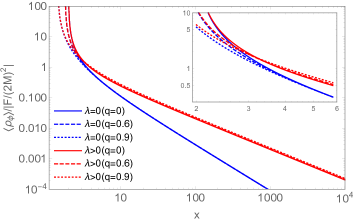
Figure 5: Comparison between the normalized energy density of the self-interacting scalar field (see Eq (32) in Ravanal et al. (2023)) in red and the non-interacting one (33) in blue, as a function of the radial coordinate $x$ for $q=0,0.6,0.9$. Here $\lambda$ represents the self-interaction of the SF. The small zoom corresponds to the region between $x_{\text{h}}$ and $x_{\text{isco}}$.

III.0.2 Axion-like dark matter particles

As a proof of concept, we compare the SF profile in different particle mass regimes, covering a wide class of SF dark matter scenarios. We pay particular attention to the large mass limit. Unfortunately, since the charged case has not been examined in such cases, we must restrict this comparison to the Schwarzschild BH. Within our approach, such a comparison makes sense at large radii when the term $Q^{2}/r^{2}$ can be safely ignored. Several authors have previously examined the massive Klein-Gordon equation Unruh (1976); Detweiler (1980). The exact solutions to this equation can be expressed in terms of the confluent Heun function Fiziev (2006a, b); Bezerra et al. (2014); Vieira et al. (2014); Konoplya and Zhidenko (2006); Barranco et al. (2012). This problem has been revisited by Hui et al. (2019) and recently extended by Bucciotti and Trincherini (2023), including the effects of angular momentum in the SF.

In the context of a BH immersed in DM, there is a possibility of developing a “scalar hair”. For a massive and oscillating non-interacting SF, the authors of Hui et al. (2019) have identified different mass regimes (see Table 1 in Hui et al. (2019)) that can distinctly impact the scalar field profile. Regime IV corresponds to $m>r_{\text{h}}^{-1}$, while Regime III is identified with $(r_{\text{sg}}r_{\text{h}})^{-1/2}\lesssim m\lesssim r_{\text{h}}^{-1}$. Furthermore, they divided the surroundings of the BH into two clearly defined regions: the first region is dominated by the BH’s geometry, extending up to a self-gravitating radius $r_{\text{sg}}$, while the second region lies beyond this point. Our large-mass regime ($r_{\text{h}}\gg 1/m$) corresponds indeed to the particle limit (regime IV in their prescription). Accordingly, they obtained the following expression for the SF profile

$$r_{\text{h}}\lesssim r\lesssim r_{\text{sg}}\;\;:\;\;\phi\thicksim r^{-3/4}\mathrm{e}^{-imt}\mathrm{e}^{-i2m\sqrt{rr_{h}}}.$$ (37)

We can observe that the amplitude of the SF profile behaves in the same way as in our case Eq. (30), as it follows the same power law $\phi\propto r^{-3/4}$. The regime III is particularly interesting because it encompasses both particle-like and wave-like behavior

$$m^{-2}r_{\text{h}}^{-1}\lesssim r\lesssim r_{\text{sg}}:\phi\thicksim r^{-3/4}\mathrm{e}^{-imt}\cos\>(2m\sqrt{rr_{h}}-3\pi/4).$$ (38)

In fact, its amplitude exhibits the same behavior as $\phi\propto r^{-3/4}$, but with an additional modulation. They obtained a density profile $\rho\propto r^{-3/2}$. This profile is interpreted as a constant and steady energy flow falling into the BH at a velocity $v_{r}\propto r^{-1/2}$, which aligns with the behavior identified in Eq. (33). As an aside, in the regime of small mass, the aforementioned author asserts that the SF profile behaves according to the power law $\phi\propto r^{-1}$, as in the Jacobson’s preliminary result Jacobson (1999).

As noted in Bucciotti and Trincherini (2023), in the large mass regime and for distances far from the BH, the SF profile is independent of the angular momentum, as it follows the same power law $\phi\propto r^{-3/4}$ (see Eq. (2.19) in Bucciotti and Trincherini (2023)). In the same direction, the authors of Clough et al. (2019) numerically calculated the SF profile in the large mass regime, considering the backreaction of the SF, and found that at significant distances from the BH, the envelopes of the SF profile follow the same power law $\phi\propto r^{-3/4}$ (see Fig. 1 in Clough et al. (2019)).

IV DISCUSSION AND CONCLUSION

The last decade has been thrilling in terms of astrophysical observations, reaching unprecedented resolutions, even on the order of the event horizon. These observations, conducted in the strong field regime, have the potential to provide unique insights not only into the intrinsic properties of BHs but also into the environments they inhabit. A key assumption in this context is the potential influence of DM on these observations, leaving distinctive signatures that could contribute to unveiling its elusive nature.

Therefore, it is of vital importance to develop models that deviate from the Schwarzschild paradigm. In this line of thinking, our study is situated, addressing the non-interactive case of the SF model and exploring the impact of electric charge $Q$ on the behavior of SF around a RN-BH. All of this is coupled with the results obtained by the EHT collaboration, which leaves open the possibility that BHs may have a non-zero electric charge. In general terms, with a 2$\sigma$ confidence level, this electric charge is found in an approximate range of $q=Q/M\in[0,0.9]$. Therefore, we limit ourselves to considering these constraints and connect these results with our previous research Ravanal et al. (2023).

The effect of $Q$ becomes relevant in the vicinity of the BH, especially in the region where marginally bound orbits are located, as shown in Fig. (1) and Fig. (3). As expected, this effect diminishes due to the $r^{-2}$ term present in the metric function $f$ and becomes less relevant as we move away from the RN-BH. At such distances, the scalar field profile decreases as $\phi\propto r^{-3/4}$, while the density profile decreases as $\rho\propto r^{-3/2}$ and the radial velocity as $v_{r}\propto r^{-1/2}$.

A notable fact is the change in slope in the density profile between the non-interactive and interactive cases, with the behavior of the latter being proportional to $r^{-1}$, and its radial velocity also following suit. This change is due to the nature of the fields, as the repulsive self-interaction slows down the fall of DM. Additionally, we require a steady-state behavior for the flow of the fields, so it must be independent of $r$. These values fall within the range typically considered by different models of power-law exponents for DM density profiles $\rho_{\text{DM}}\propto r^{-\gamma}$ for $\gamma$ $\in[0,5]$ Ferreira (2021).

An interesting inference is uncovered from Fig. (5): the charge has a non-trivial impact on the density profile within marginally bound orbits. This leads us to the question: is it possible to extract information about the DM properties from BH observations within a beyond the Schwarzschild geometry? At first glance, it seems very challenging, but with the upcoming high-resolution BH experiments in the strong-field scale, we expect to detect the famous “scalar hair” and characterize the spacetime geometry unprecedentedly.

We found that the maximum accretion rate of the SF in marginally bound orbits, i.e., between $r_{\text{mb}}$ and $r_{\text{isco}}$, decreases by up to 50 % in the case of maximum allowed charge compared to the uncharged scenario. The choice of $r_{\text{mb}}$ as the upper limit is based on the premise that, with the SF having a nonzero mass, the capture of particles in these orbits is more probable and the fall into the BH seems inevitable, as there is no point of return once entering that radius. We also obtained an order of magnitude estimate for the accretion of SF dark matter $\dot{M}_{\text{SFDM}}\thicksim 10^{-8}M_{\odot}\;\text{yr}^{-1}$, which is higher compared to the self-interacting case $\dot{M}_{\rm SIDM}\sim 10^{-10}M_{\odot}~{}{\rm yr}^{-1}$ Ravanal et al. (2023). In both cases, the value is small compared to the usual accretion of baryons (Bondi or Eddington) reported in previous research Salpeter (1964); Bondi and Hoyle (1944); Bondi (1952); Edgar (2004); Akiyama et al. (2021). This relatively small number leaves open the possibility that structures at the subgalactic or galactic level composed of DM continue to exist at present times, as these structures are typically estimated to have hundreds of thousands or millions of solar masses.

In summary, current and future observations of BHs provide a unique opportunity to investigate the role that DM plays in the dynamics of these cosmic objects and their surroundings. These observations, supported by theoretical advances, have the potential to shed light on the nature of DM and its interactions with BHs. Although our study is modest, it has provided a different perspective, often overlooked, on the impact of electric charge on BHs and its secular effect in the vicinity. We hope that our findings open new avenues for future research in this fascinating field, contributing to the understanding of this elusive component of our Universe.

V ACKNOWLEDGEMENTS

Y. R is supported by Beca Doctorado Convenio Marco de la Universidad de Santiago de Chile (USACH) from 2019-2020 and by Beca Doctorado Nacional año 2021 Folio No. 21211644 de la Agencia Nacional de Investigacion y Desarrollo de Chile (ANID). G. G acknowledges financial support from Agencia Nacional de Investigación y Desarrollo (ANID), Chile, through the FONDECYT postdoctoral Grant No. 3210417. N.C acknowledges the support of Universidad de Santiago de Chile (USACH), through Proyecto DICYT N° 042131CM, Vicerrectoría de Investigación, Desarrollo e Innovación.

*

References

- Spergel et al. (2003) D. N. Spergel et al. (WMAP), Astrophys. J. Suppl. 148, 175 (2003), arXiv:astro-ph/0302209 .
- Ade et al. (2016) P. A. R. Ade et al. (Planck), Astron. Astrophys. 594, A13 (2016), arXiv:1502.01589 [astro-ph.CO] .
- Aghanim et al. (2020) N. Aghanim et al. (Planck), Astron. Astrophys. 641, A6 (2020), [Erratum: Astron.Astrophys. 652, C4 (2021)], arXiv:1807.06209 [astro-ph.CO] .
- Tegmark et al. (2004) M. Tegmark et al. (SDSS), Astrophys. J. 606, 702 (2004), arXiv:astro-ph/0310725 .
- Anderson et al. (2014) L. Anderson et al. (BOSS), Mon. Not. Roy. Astron. Soc. 441, 24 (2014), arXiv:1312.4877 [astro-ph.CO] .
- Alam et al. (2017) S. Alam et al. (BOSS), Mon. Not. Roy. Astron. Soc. 470, 2617 (2017), arXiv:1607.03155 [astro-ph.CO] .
- Navarro et al. (1996) J. F. Navarro, C. S. Frenk, and S. D. M. White, Astrophys. J. 462, 563 (1996), arXiv:astro-ph/9508025 .
- Moore (1994) B. Moore, Nature 370, 629 (1994).
- de Blok (2010) W. J. G. de Blok, Adv. Astron. 2010, 789293 (2010), arXiv:0910.3538 [astro-ph.CO] .
- Oh et al. (2011) S.-H. Oh, C. Brook, F. Governato, E. Brinks, L. Mayer, W. J. G. de Blok, A. Brooks, and F. Walter, Astron. J. 142, 24 (2011), arXiv:1011.2777 [astro-ph.CO] .
- Moore et al. (1999) B. Moore, S. Ghigna, F. Governato, G. Lake, T. R. Quinn, J. Stadel, and P. Tozzi, Astrophys. J. Lett. 524, L19 (1999), arXiv:astro-ph/9907411 .
- Bullock et al. (2000) J. S. Bullock, A. V. Kravtsov, and D. H. Weinberg, Astrophys. J. 539, 517 (2000), arXiv:astro-ph/0002214 .
- Boylan-Kolchin et al. (2011) M. Boylan-Kolchin, J. S. Bullock, and M. Kaplinghat, Mon. Not. Roy. Astron. Soc. 415, L40 (2011), arXiv:1103.0007 [astro-ph.CO] .
- Garrison-Kimmel et al. (2014) S. Garrison-Kimmel, M. Boylan-Kolchin, J. S. Bullock, and E. N. Kirby, Mon. Not. Roy. Astron. Soc. 444, 222 (2014), arXiv:1404.5313 [astro-ph.GA] .
- Del Popolo and Le Delliou (2017) A. Del Popolo and M. Le Delliou, Galaxies 5, 17 (2017), arXiv:1606.07790 [astro-ph.CO] .
- Dutton et al. (2019) A. A. Dutton, A. V. Macciò, T. Buck, K. L. Dixon, M. Blank, and A. Obreja, Mon. Not. Roy. Astron. Soc. 486, 655 (2019), arXiv:1811.10625 [astro-ph.GA] .
- Dutton et al. (2020) A. A. Dutton, T. Buck, A. V. Macciò, K. L. Dixon, M. Blank, and A. Obreja, (2020), 10.1093/mnras/staa3028, arXiv:2011.11351 [astro-ph.GA] .
- Sommer-Larsen and Vedel (1999) J. Sommer-Larsen and H. Vedel, Astrophys. J. 519, 501 (1999), arXiv:astro-ph/9801094 .
- Milgrom (1983) M. Milgrom, Astrophys. J. 270, 365 (1983).
- Hu et al. (2000) W. Hu, R. Barkana, and A. Gruzinov, Phys. Rev. Lett. 85, 1158 (2000), arXiv:astro-ph/0003365 .
- Hui et al. (2017) L. Hui, J. P. Ostriker, S. Tremaine, and E. Witten, Phys. Rev. D 95, 043541 (2017), arXiv:1610.08297 [astro-ph.CO] .
- Ferreira (2021) E. G. M. Ferreira, Astron. Astrophys. Rev. 29, 7 (2021), arXiv:2005.03254 [astro-ph.CO] .
- Sin (1994) S.-J. Sin, Phys. Rev. D 50, 3650 (1994), arXiv:hep-ph/9205208 .
- Ji and Sin (1994) S. U. Ji and S. J. Sin, Phys. Rev. D 50, 3655 (1994), arXiv:hep-ph/9409267 .
- Seidel and Suen (1990) E. Seidel and W.-M. Suen, Phys. Rev. D 42, 384 (1990).
- Matos and Guzman (2000) T. Matos and F. S. Guzman, Class. Quant. Grav. 17, L9 (2000), arXiv:gr-qc/9810028 .
- Hui et al. (2019) L. Hui, D. Kabat, X. Li, L. Santoni, and S. S. C. Wong, JCAP 06, 038 (2019), arXiv:1904.12803 [gr-qc] .
- Dave and Goswami (2023) B. Dave and G. Goswami, (2023), arXiv:2304.04463 [astro-ph.CO] .
- Goodman (2000) J. Goodman, New Astron. 5, 103 (2000), arXiv:astro-ph/0003018 .
- Peebles (2000) P. J. E. Peebles, Astrophys. J. Lett. 534, L127 (2000), arXiv:astro-ph/0002495 .
- Arbey et al. (2003) A. Arbey, J. Lesgourgues, and P. Salati, Phys. Rev. D 68, 023511 (2003), arXiv:astro-ph/0301533 .
- Boehmer and Harko (2007) C. G. Boehmer and T. Harko, JCAP 06, 025 (2007), arXiv:0705.4158 [astro-ph] .
- Lee and Lim (2010) J.-W. Lee and S. Lim, JCAP 01, 007 (2010), arXiv:0812.1342 [astro-ph] .
- Harko (2011) T. Harko, JCAP 05, 022 (2011), arXiv:1105.2996 [astro-ph.CO] .
- Rindler-Daller and Shapiro (2012) T. Rindler-Daller and P. R. Shapiro, Mon. Not. Roy. Astron. Soc. 422, 135 (2012), arXiv:1106.1256 [astro-ph.CO] .
- Suárez et al. (2014) A. Suárez, V. H. Robles, and T. Matos, Astrophys. Space Sci. Proc. 38, 107 (2014), arXiv:1302.0903 [astro-ph.CO] .
- Ureña López (2019) L. A. Ureña López, Front. Astron. Space Sci. 6, 47 (2019).
- Peccei and Quinn (1977) R. D. Peccei and H. R. Quinn, Phys. Rev. Lett. 38, 1440 (1977).
- Wilczek (1978) F. Wilczek, Phys. Rev. Lett. 40, 279 (1978).
- Weinberg (1978) S. Weinberg, Phys. Rev. Lett. 40, 223 (1978).
- Marsh (2016) D. J. E. Marsh, Phys. Rept. 643, 1 (2016), arXiv:1510.07633 [astro-ph.CO] .
- Kobayashi et al. (2017) T. Kobayashi, R. Murgia, A. De Simone, V. Iršič, and M. Viel, Phys. Rev. D 96, 123514 (2017), arXiv:1708.00015 [astro-ph.CO] .
- Abel et al. (2017) C. Abel et al., Phys. Rev. X 7, 041034 (2017), arXiv:1708.06367 [hep-ph] .
- Brito et al. (2017a) R. Brito, S. Ghosh, E. Barausse, E. Berti, V. Cardoso, I. Dvorkin, A. Klein, and P. Pani, Phys. Rev. Lett. 119, 131101 (2017a), arXiv:1706.05097 [gr-qc] .
- Brito et al. (2017b) R. Brito, S. Ghosh, E. Barausse, E. Berti, V. Cardoso, I. Dvorkin, A. Klein, and P. Pani, Phys. Rev. D 96, 064050 (2017b), arXiv:1706.06311 [gr-qc] .
- Arbey et al. (2001) A. Arbey, J. Lesgourgues, and P. Salati, Phys. Rev. D 64, 123528 (2001), arXiv:astro-ph/0105564 .
- Schive et al. (2014) H.-Y. Schive, M.-H. Liao, T.-P. Woo, S.-K. Wong, T. Chiueh, T. Broadhurst, and W. Y. P. Hwang, Phys. Rev. Lett. 113, 261302 (2014), arXiv:1407.7762 [astro-ph.GA] .
- Marsh and Pop (2015) D. J. E. Marsh and A.-R. Pop, Mon. Not. Roy. Astron. Soc. 451, 2479 (2015), arXiv:1502.03456 [astro-ph.CO] .
- Schwabe et al. (2016) B. Schwabe, J. C. Niemeyer, and J. F. Engels, Phys. Rev. D 94, 043513 (2016), arXiv:1606.05151 [astro-ph.CO] .
- Mocz et al. (2017) P. Mocz, M. Vogelsberger, V. H. Robles, J. Zavala, M. Boylan-Kolchin, A. Fialkov, and L. Hernquist, Mon. Not. Roy. Astron. Soc. 471, 4559 (2017), arXiv:1705.05845 [astro-ph.CO] .
- Levkov et al. (2018) D. G. Levkov, A. G. Panin, and I. I. Tkachev, Phys. Rev. Lett. 121, 151301 (2018), arXiv:1804.05857 [astro-ph.CO] .
- Chavanis (2011) P.-H. Chavanis, Phys. Rev. D 84, 043531 (2011), arXiv:1103.2050 [astro-ph.CO] .
- Chavanis and Delfini (2011) P.-H. Chavanis and L. Delfini, Phys. Rev. D 84, 043532 (2011), arXiv:1103.2054 [astro-ph.CO] .
- Schneider (2015) P. Schneider, Extragalactic Astronomy and Cosmology: An Introduction (2015).
- Peebles (1969) P. J. E. Peebles, Astrophys. J. 155, 393 (1969).
- Kain and Ling (2010) B. Kain and H. Y. Ling, Phys. Rev. D 82, 064042 (2010), arXiv:1004.4692 [hep-ph] .
- Iršič et al. (2017) V. Iršič, M. Viel, M. G. Haehnelt, J. S. Bolton, and G. D. Becker, Phys. Rev. Lett. 119, 031302 (2017), arXiv:1703.04683 [astro-ph.CO] .
- Rogers and Peiris (2021) K. K. Rogers and H. V. Peiris, Phys. Rev. Lett. 126, 071302 (2021), arXiv:2007.12705 [astro-ph.CO] .
- Bar et al. (2022) N. Bar, K. Blum, and C. Sun, Phys. Rev. D 105, 083015 (2022), arXiv:2111.03070 [hep-ph] .
- Kormendy and Richstone (1995) J. Kormendy and D. Richstone, Ann. Rev. Astron. Astrophys. 33, 581 (1995).
- Ferrarese and Ford (2005) L. Ferrarese and H. Ford, Space Sci. Rev. 116, 523 (2005), arXiv:astro-ph/0411247 .
- Narayan (2005) R. Narayan, New J. Phys. 7, 199 (2005), arXiv:gr-qc/0506078 .
- Zakharov (2014) A. F. Zakharov, Phys. Rev. D 90, 062007 (2014), arXiv:1407.7457 [gr-qc] .
- Juraeva et al. (2021) N. Juraeva, J. Rayimbaev, A. Abdujabbarov, B. Ahmedov, and S. Palvanov, Eur. Phys. J. C 81, 70 (2021).
- Kocherlakota et al. (2021) P. Kocherlakota et al. (Event Horizon Telescope), Phys. Rev. D 103, 104047 (2021), arXiv:2105.09343 [gr-qc] .
- Akiyama et al. (2022) K. Akiyama et al. (Event Horizon Telescope), Astrophys. J. Lett. 930, L17 (2022).
- Vagnozzi et al. (2022) S. Vagnozzi et al., (2022), arXiv:2205.07787 [gr-qc] .
- Abbott et al. (2016) B. P. Abbott et al. (LIGO Scientific, Virgo), Phys. Rev. Lett. 116, 061102 (2016), arXiv:1602.03837 [gr-qc] .
- Eda et al. (2013) K. Eda, Y. Itoh, S. Kuroyanagi, and J. Silk, Phys. Rev. Lett. 110, 221101 (2013), arXiv:1301.5971 [gr-qc] .
- Lacroix and Silk (2013) T. Lacroix and J. Silk, Astron. Astrophys. 554, A36 (2013), arXiv:1211.4861 [astro-ph.GA] .
- Kavanagh et al. (2020) B. J. Kavanagh, D. A. Nichols, G. Bertone, and D. Gaggero, Phys. Rev. D 102, 083006 (2020), arXiv:2002.12811 [gr-qc] .
- Gómez et al. (2016) L. G. Gómez, C. R. Argüelles, V. Perlick, J. A. Rueda, and R. Ruffini, Phys. Rev. D 94, 123004 (2016), arXiv:1610.03442 [astro-ph.GA] .
- Bar et al. (2019) N. Bar, K. Blum, T. Lacroix, and P. Panci, JCAP 07, 045 (2019), arXiv:1905.11745 [astro-ph.CO] .
- Saurabh and Jusufi (2021) K. Saurabh and K. Jusufi, Eur. Phys. J. C 81, 490 (2021), arXiv:2009.10599 [gr-qc] .
- Boudon et al. (2023) A. Boudon, P. Brax, P. Valageas, and L. K. Wong, (2023), arXiv:2305.18540 [astro-ph.CO] .
- Chakrabarti et al. (2022) S. Chakrabarti, B. Dave, K. Dutta, and G. Goswami, JCAP 09, 074 (2022), arXiv:2202.11081 [astro-ph.CO] .
- Sadeghian et al. (2013) L. Sadeghian, F. Ferrer, and C. M. Will, Phys. Rev. D 88, 063522 (2013), arXiv:1305.2619 [astro-ph.GA] .
- Barranco et al. (2011) J. Barranco, A. Bernal, J. C. Degollado, A. Diez-Tejedor, M. Megevand, M. Alcubierre, D. Nunez, and O. Sarbach, Phys. Rev. D 84, 083008 (2011), arXiv:1108.0931 [gr-qc] .
- Clough et al. (2019) K. Clough, P. G. Ferreira, and M. Lagos, Phys. Rev. D 100, 063014 (2019), arXiv:1904.12783 [gr-qc] .
- Bamber et al. (2021) J. Bamber, K. Clough, P. G. Ferreira, L. Hui, and M. Lagos, Phys. Rev. D 103, 044059 (2021), arXiv:2011.07870 [gr-qc] .
- Aguilar-Nieto et al. (2023) A. Aguilar-Nieto, V. Jaramillo, J. Barranco, A. Bernal, J. C. Degollado, and D. Núñez, Phys. Rev. D 107, 044070 (2023), arXiv:2211.10456 [gr-qc] .
- Brax et al. (2020) P. Brax, J. A. R. Cembranos, and P. Valageas, Phys. Rev. D 101, 023521 (2020), arXiv:1909.02614 [astro-ph.CO] .
- Vicente and Cardoso (2022) R. Vicente and V. Cardoso, Phys. Rev. D 105, 083008 (2022), arXiv:2201.08854 [gr-qc] .
- Cardoso et al. (2022) V. Cardoso, T. Ikeda, R. Vicente, and M. Zilhão, Phys. Rev. D 106, L121302 (2022), arXiv:2207.09469 [gr-qc] .
- Jacobson (1999) T. Jacobson, Phys. Rev. Lett. 83, 2699 (1999), arXiv:astro-ph/9905303 .
- Brihaye and Hartmann (2022) Y. Brihaye and B. Hartmann, Class. Quant. Grav. 39, 015010 (2022), arXiv:2108.02248 [gr-qc] .
- Unruh (1976) W. G. Unruh, Phys. Rev. D 14, 3251 (1976).
- Detweiler (1980) S. L. Detweiler, Phys. Rev. D 22, 2323 (1980).
- Benone et al. (2014) C. L. Benone, E. S. de Oliveira, S. R. Dolan, and L. C. B. Crispino, Phys. Rev. D 89, 104053 (2014), arXiv:1404.0687 [gr-qc] .
- Reissner (1916) H. Reissner, Annalen der Physik 355, 106 (1916).
- Ravanal et al. (2023) Y. Ravanal, G. Gómez, and N. Cruz, Phys. Rev. D 108, 083004 (2023), arXiv:2306.10204 [astro-ph.CO] .
- Feng et al. (2022) W.-X. Feng, A. Parisi, C.-S. Chen, and F.-L. Lin, JCAP 08, 032 (2022), arXiv:2112.05160 [astro-ph.HE] .
- Gómez and Valageas (2024) G. Gómez and P. Valageas, (2024), arXiv:2403.08988 [astro-ph.CO] .
- Bucciotti and Trincherini (2023) B. Bucciotti and E. Trincherini, (2023), arXiv:2309.02482 [hep-th] .
- Brax et al. (2019) P. Brax, J. A. R. Cembranos, and P. Valageas, Phys. Rev. D 100, 023526 (2019), arXiv:1906.00730 [astro-ph.CO] .
- Akiyama et al. (2021) K. Akiyama et al. (Event Horizon Telescope), Astrophys. J. Lett. 910, L13 (2021), arXiv:2105.01173 [astro-ph.HE] .
- Madelung (1927) E. Madelung, z. Phys 40, 322 (1927).
- Shapiro and Teukolsky (1983) S. L. Shapiro and S. A. Teukolsky, Black holes, white dwarfs, and neutron stars: The physics of compact objects (1983).
- Gondolo and Silk (1999) P. Gondolo and J. Silk, Phys. Rev. Lett. 83, 1719 (1999), arXiv:astro-ph/9906391 .
- Pugliese et al. (2011) D. Pugliese, H. Quevedo, and R. Ruffini, Phys. Rev. D 83, 024021 (2011), arXiv:1012.5411 [astro-ph.HE] .
- Beheshti and Gasperin (2016) S. Beheshti and E. Gasperin, Phys. Rev. D 94, 024015 (2016), arXiv:1512.08707 [gr-qc] .
- Gómez and Rodríguez (2023) G. Gómez and J. F. Rodríguez, Phys. Rev. D 108, 024069 (2023), arXiv:2301.05222 [gr-qc] .
- Kovacic and Brennan (2011) I. Kovacic and M. J. Brennan, The Duffing equation: nonlinear oscillators and their behaviour (John Wiley & Sons, 2011).
- Frasca (2011) M. Frasca, J. Nonlin. Math. Phys. 18, 291 (2011), arXiv:0907.4053 [math-ph] .
- Fiziev (2006a) P. P. Fiziev, Class. Quant. Grav. 23, 2447 (2006a), arXiv:gr-qc/0509123 .
- Fiziev (2006b) P. P. Fiziev, (2006b), arXiv:gr-qc/0603003 .
- Bezerra et al. (2014) V. B. Bezerra, H. S. Vieira, and A. A. Costa, Class. Quant. Grav. 31, 045003 (2014), arXiv:1312.4823 [gr-qc] .
- Vieira et al. (2014) H. S. Vieira, V. B. Bezerra, and C. R. Muniz, Annals Phys. 350, 14 (2014), arXiv:1401.5397 [gr-qc] .
- Konoplya and Zhidenko (2006) R. A. Konoplya and A. Zhidenko, Phys. Rev. D 73, 124040 (2006), arXiv:gr-qc/0605013 .
- Barranco et al. (2012) J. Barranco, A. Bernal, J. C. Degollado, A. Diez-Tejedor, M. Megevand, M. Alcubierre, D. Nunez, and O. Sarbach, Phys. Rev. Lett. 109, 081102 (2012), arXiv:1207.2153 [gr-qc] .
- Salpeter (1964) E. E. Salpeter, Astrophys. J. 140, 796 (1964).
- Bondi and Hoyle (1944) H. Bondi and F. Hoyle, Mon. Not. Roy. Astron. Soc. 104, 273 (1944).
- Bondi (1952) H. Bondi, Mon. Not. Roy. Astron. Soc. 112, 195 (1952).
- Edgar (2004) R. G. Edgar, New Astron. Rev. 48, 843 (2004), arXiv:astro-ph/0406166 .