Synchronization Conditions for Nonlinear Oscillator Networks

Abstract

Understanding conditions for the synchronization of a network of interconnected oscillators is a challenging problem. Typically, only sufficient conditions are reported for the synchronization problem. Here, we adopted the Lyapunov-Floquet theory and the Master Stability Function approach in order to derive the synchronization conditions for a set of coupled nonlinear oscillators. We found that the positivity of the coupling constant is a necessary and sufficient condition for synchronizing linearly full-state coupled identical oscillators. Moreover, in the case of partial state coupling, the asymptotic convergence of volume in state space is ensured by a positive coupling constant. The numerical calculation of the Master Stability Function for a benchmark two-dimensional oscillator validates the synchronization corresponding to the positive coupling. The results are illustrated using numerical simulations and experimentation on benchmark oscillators.

I Introduction

Synchronization of oscillators is a phenomenon that occurs in a wide variety of natural and engineered contexts. Examples include synchronized oscillations in biology [1, 2, 3, 4], neuroscience [5, 6, 7, 8], and electronics [9, 10, 11, 12, 13, 14]. Understanding conditions for synchronization to occur would benefit their analysis and design.

A significant advance in obtaining conditions for synchronization was the Master Stability Function approach [15]. Through a computation of the Floquet multipliers of nodes of a network of oscillators, conditions for synchronization could be verified numerically. There have been several attempts to obtain theoretical conditions for synchronization [16, 17, 18, 19, 20, 21, 22, 23], but these are often conservative and provide only sufficient conditions. For example, the synchronization condition in the case of coupled Van der Pol oscillators, obtained using a Lyapunov function approach and a contraction theory-based approach, is that the critical coupling gain depends on the system parameter and the connectivity graph.

In addition to numerical studies, electronic implementations of oscillator networks have been investigated as more realistic models that often show rich dynamics [12, 13, 11, 23, 24, 25]. These studies provide important foundations for the analysis and design of synchronization. However, the problem of obtaining tighter bounds on the coupling strength for an oscillator network is generally unresolved.

Here, we aim to obtain the synchronizing condition for a set of coupled nonlinear oscillators. To derive these conditions, we used the Lyapunov-Floquet Theory and the Master Stability Function approach. The key finding is that the positivity of the coupling constant is a necessary and sufficient condition for the synchronization of a network of identical oscillators connected linearly in a full-state fashion. A positive coupling constant assures that the volume in the state space converges to zero asymptotically for a set of oscillators with partial state linear coupling. Moreover, a numerical computation of the Master Stability Function for a benchmark two-dimensional oscillator confirm the synchronization behavior for positive coupling. These findings are demonstrated on benchmark oscillators by numerical simulations, LT SPICE, and electronic implementation.

II Mathematical Background

This section provides a brief overview of the relevant mathematical theory that is used in this study. Consider a nonlinear dynamical system

$$\dot{x}_{i}=f\left(x_{i}\right),\text{ }x_{i}\in\mathbb{R}^{m},$$ (1)

with a limit cycle $x_{s}(t)$ with time period $T$. Linearizing this system around $x=x_{s}(t)$ gives the linear time-periodic system

$$\dot{y}=A(t)y,\text{ }y\in\mathbb{R}^{m},$$ (2)

$A(t)=Df(x_{s}(t))$, where $Df$ is the Jacobian of $f$ at $x(t)=x_{s}(t)$.

II-A Floquet Theory

Floquet theory was developed to describe the behavior of a system of linear differential equations with time-periodic coefficients [26]. The theory introduces the concept of the Floquet multipliers ($\mu$), which are eigenvalue-like entities that describe the exponential growth or decay of solutions over one time period of the system. The fundamental solutions denote the state transition by $\phi(t,t_{0})$. Define $R$ by $e^{RT}=\phi(T,0)$ and $P^{-1}(t)=\phi(t,0)e^{-RT}$. Then $P^{-1}(t)$ is periodic with period $T$ as $P^{-1}(t+T)=\phi(t+T,0)e^{-R(t+T)}=\phi(t+T,T).\phi(T,0).e^{-RT}.e^{-Rt}=\phi(t,0).e^{-Rt}=P^{-1}(t)$. In the co-ordinates $z=P(t)y$, the system is the linear time invariant system $\dot{z}=Rz$ as $\dot{P}(t)P^{-1}(t)+P(t)A(t)P^{-1}(t)=R.$ The eigenvalues of $R$, called the Floquet exponents, determine the stability. Floquet multipliers are the eigenvalues of $e^{RT}$. For asymptotic stability, one of the Floquet multiplier has absolute value as $1$, representing perturbations along the limit cycle, and others have moduli strictly less than $1$.

II-B Master Stability Function

Consider $n$ identical oscillators

$$\dot{x}_{i}=f\left(x_{i}\right),\text{ }x_{i}\in\mathbb{R}^{m},\text{ }i\in\{1,2,...,n\},$$ (3)

diffusively and identically coupled in a fully connected network

$$\dot{x}_{i}=f\left(x_{i}\right)+K\sum_{j\in{N_{i}}}G_{ij}H\left(x_{j}\right),$$ (4)

where $K$ is the coupling constant, $N_{i}$ is the neighborhood of the oscillator $i$, $G=[a_{ij}]$ is the graph Laplacian and $H$ is an matrix containing information on the coupled variables. For linear coupling, the coupling between an oscillator $i$ and an oscillator $j\in N_{i}$ is $K(x_{j}-x_{i})$. A simplified representation is

$$\dot{X}=I_{n}\otimes f(X)+KG\otimes H(X),$$ (5)

where $X=\left[x_{1}^{T},x_{2}^{T},\ldots,x_{n}^{T}\right]^{T}$ is a $nm$-dimensional state vector, and $\otimes$ is the Kronecker product. Linearisation around the state $X_{s}=\left[x_{s}^{T},x_{s}^{T},\ldots,x_{s}^{T}\right]^{T}$ yields

$$\dot{Y}=\left[I_{n}\otimes Df\left(x_{s}\right)-KG\otimes DH\left(x_{s}\right)\right]Y,$$ (6)

where $DH(x_{s})$ is the Jacobian of $H$ at $x(t)=x_{s}(t)$. Equation (6) can be written in block matrix form by introducing a transformation $\zeta=(Q\otimes I_{n})Y$, where $Q$ is the transformation matrix. On diagonalising $G$ through the transformation $Q$, where $Q^{-1}GQ=\text{diag}\left[0,\lambda_{2},\lambda_{3},...,\lambda_{n}\right]$, $0<\lambda_{2}\leq\lambda_{3}\leq,...,\leq\lambda_{n}$. In transformed co-ordinates, the dynamics are in block form, with each block representing an eigenmode

$$\dot{\zeta_{i}}=[DF\left(x_{s}\right)-K\lambda_{i}DH\left(x_{s}\right)]\zeta_{i},\text{ }i=1,2,...,n.$$ (7)

$\zeta_{i}$ is referred as the synchronization mode. The dynamics corresponding to the first eigenmode is $\dot{\zeta}_{1}=DF(x_{S})\zeta_{1}$, which is the same as the linearised dynamics around the limit cycle. Assuming this mode to be stable, the stability of the synchronized state is determined by Floquet multipliers of all other eigenmodes. The Master Stability Function ($\mu_{max}(\lambda)$) is the largest non-unity Floquet multiplier of the system matrix $[DF\left(x_{s}\right)-K\lambda DH\left(x_{s}\right)]$. The necessary and sufficient condition for the stability of the limit cycle is $\mu_{max}(\lambda)<1$.

III Condition For Synchronization

This section investigates the condition for synchronization of identical oscillators coupled identically and linearly. Synchronization of two or more identical oscillators is defined as the situation when the difference between their corresponding states is asymptotically zero.

Theorem 1

A network of identical oscillators (4) coupled identically and linearly in full-state fashion synchronizes if and only if $K>0$.

Proof:

The proof relies on the Lyapunov-Floquet transformation $P(t)\in\mathbb{R}^{m\times m}$ [27] and the fact that for identical linear full-state coupling, $DH=I.$ Applying the transformation $P(t)$ at each eigenmode $\lambda_{i}$ (refer (7)) results in

$$\dot{Z}_{i}=(R-KP(t)DH(x_{s})P^{-1}(t))Z_{i},\text{ }i=1,2,...,n,$$ (8)

$$\dot{Z}_{i}=(R-K\lambda_{i}I)Z_{i},\text{ }i=1,2,...,n,$$ (9)

where $R$ is defined in subsection II-A. For $K=0$, system dynamics (7) become uncoupled, and the matrix $R\in\mathbb{R}^{m\times m}$ has one eigenvalue at $0$ and other $(m-1)$ eigenvalues with strictly negative real parts. For coupled dynamics in (9), the eigenvalues are the roots of the polynomial,

$$\det(sI-(R-K\lambda_{i}I))=0,$$

$$\Rightarrow\det((s+K\lambda_{i})I-R)=0.$$

The roots of the above characteristic equation depend on the coupling strength $K$ and the eigenmode $\lambda_{i}$. To prove sufficiency, first assume that $K>0$ and define $s+K\lambda_{i}=\alpha\text{ }\Rightarrow s=\alpha-K\lambda_{i}$. For $K=0,\text{ }s=\alpha$, and the eigenvalues are same as those of $R$. One can conclude that the set of eigenvalues of $(R-K\lambda_{i}I)$ are the same as the set of the eigenvalues of $R$ except offset by $-K\lambda_{i}$. All eigenvalues of $R$ corresponding to each synchronization modes ($\lambda_{i}$) have a strictly negative real part except for one eigenvalue of the first eigenmode ($\lambda_{1}=0$), which is zero.

To prove the necessary condition, we suppose that $K<0$. Define $s+K\lambda_{i}=\alpha\text{ }\Rightarrow s=\alpha-K\lambda_{i}$. We use the method of contradiction and assume that the synchronization is achieved if $K<0$. The matrix $R\in\mathbb{R}^{m\times m}$ has one eigenvalue $0$ and other $(m-1)$ eigenvalues with strictly negative real parts. However, as $K<0$, the first eigenvalue of matrix $R$, which is zero, moves to the right half of the complex plane for all eigenmode $\lambda_{i}$, ($i=2,...,n$). It means that at least one of the eigenvalues of ($R-K\lambda_{i}I$) corresponding to $i^{th}$ eigenmode has a positive real part. This contradicts the supposition. ∎

Remark 1

Using the Lyapunov-Floquet transformation, the necessary and sufficient condition on the coupling gain $K$ for the synchronization of $n$ oscillators has been obtained to be $K>0$. This condition is non-conservative as compare to existing results. For example, using a contraction theory-based approach, a sufficient condition for the synchronization of $n$ coupled oscillators was found to be $K>\frac{\alpha}{n}$, where $\alpha$ is an upper bound of a matrix measure of the associated Jacobian [17]. Moreover, using a Lyapunov function-based approach, a similar sufficient condition for the synchronization of $n$ coupled Van der Pol oscillators was found to be $K>\mu/n$, where $\mu$ is the system parameter[23].

Theorem 1 is derived in the case that all states are coupled. When only some states are coupled (referred to as a partially coupled system). In general, $DH=diag[d_{1},d_{2},...,d_{n}]$ where $d_{i}\in\{0,1\}$ $i=1,2,...,n$ and not all $d_{i}=1$ simultaneously. The above proof doesn’t work because the matrix multiplication of $P(t)$ and $DH$ is not necessarily commutative. However, a sufficient condition on the time evolution of the determinant of the state transition matrix is obtained using Abel-Jacobi-Liouville (AJL) identity [28].

Theorem 2

For the network of identical oscillators (4) coupled linearly in a partial state fashion, $K>0$ implies $\lim\limits_{t\to\infty}\operatorname{det}\phi(t,t_{0})=0$, where $\phi(t,t_{0})$ is the state transition matrix of (7).

Proof:

The AJL identity for an uncoupled system (2) is

$$\operatorname{det}\phi\left(t,t_{0}\right)=\exp\left[\int_{t_{0}}^{t}{\operatorname{tr}(DF(x_{s}(\tau))d\tau)}\right],$$ (10)

where $\operatorname{det}\phi\left(t,t_{0}\right)$ is the state transition matrix. The determinant of the transition matrix can be interpreted as a measure of the volume in the phase space. For the linearized partial state coupled system (7), the state transition matrix corresponding to each eigenmode follows

$$\operatorname{det}\phi\left(t,t_{0}\right)=\exp\left[\int_{t_{0}}^{t}{\operatorname{tr}(DF(x_{s}(\tau))-K\lambda_{i}DH(x_{s}))d\tau}\right],$$ (11)

$$=\exp\left[\int_{t_{0}}^{t}{(\operatorname{tr}(DF(x_{s}(\tau)))d\tau)}\right]\exp(-K\lambda_{i}(t-t_{0})).$$ (12)

For positive coupling gain $K>0$, (12) ensures the convergence of $\operatorname{det}\phi\left(t,t_{0}\right)$. In other words, for positive values of $K$, $\operatorname{det}\phi\left(t,t_{0}\right)$ $\rightarrow 0$ as $t\rightarrow\infty$. ∎

We further used a numerical approach to study the synchronization behavior of a second-order partial-state coupled system (7). For this purpose, the Master Stability Function was calculated numerically [15]. We found the maximum Floquet multiplier is a decreasing function of the coupling strength ($K$). This has been shown in Fig. 1. As the maximum Floquet multiplier is less than one for $K>0$, the computation suggests synchronization.

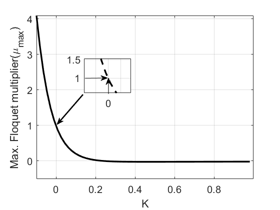
Figure 1: Numerical computation of the Master Stability Function for a coupled Van der Pol oscillator shows that the maximum Floquet multiplier decreases as the coupling strength ($K$) increases. Calculating the Floquet multiplier numerically required calculating the period and limit cycle. Solve the matrix differential equation over one period given the Identity matrix as the initial condition

IV Numerical Simulations

The present section uses numerical simulations to report the synchronization behavior for both full-state and partial-state coupling. Here, oscillators were coupled linearly. As case studies, two benchmark oscillators are considered— the Van der Pol oscillator [2] and the repressilator [29, 30, 31].

Example 1: Van der Pol oscillator. The Van der Pol oscillator is a nonlinear oscillator that exhibits limit cycle behavior and is frequently employed to simulate self-sustained oscillations. This oscillator describes the behavior of a nonlinearly damped oscillator and is modeled as

$$\begin{split}\dot{x}_{1}&=x_{2},\\ \dot{x}_{2}&=\mu(1-x_{1}^{2})x_{2}-x_{1},\end{split}$$

where $\mu$ is a parameter. We investigated synchronization for a coupling gain $K>0$. The graph Laplacian and the linearized coupling matrix of three coupled oscillators with full-state coupling are, respectively

$$G=\begin{pmatrix}2&-1&-1\\ -1&2&-1\\ -1&-1&2\end{pmatrix}\text{ and }DH=\textbf{I}_{2\times 2}.$$ (13)

We denote $x_{ij}$ as the $j^{th}$ state of the $i^{th}$ oscillator, where $j\in\{1,2\}$ and $i\in\{1,2,3\}$. In the absence of coupling, all three oscillators oscillate independently between $0-20$ sec ( Fig. 2(a)). After $20$ sec, the coupling gain ($K=1$) is turned on, and the oscillators get synchronized (Fig. 2(a)).

In partial-state coupling, the graph Laplacian matrix of coupled three oscillators was the same as (13), but the linearized coupling matrix $DH$ was $\begin{pmatrix}0&0\\ 0&1\end{pmatrix},$ This means that only the second state from each oscillator is coupled. As the coupling gain ($K=1$) is turned on at $t=20$sec, all three oscillators get synchronized (Fig. 2(b)).

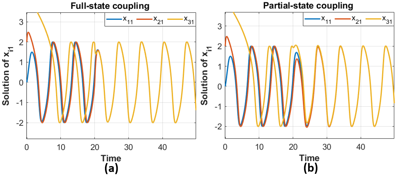
Figure 2: Numerical simulation of three coupled Van der Pol oscillators for $\mu=1$, $\text{initial condition:}(x_{10}=[0,1],x_{20}=[2,3],x_{30}=[4,5])$ and $K=1$. (a) Synchronization with full-state coupling. (b) Synchronization with partial-state coupling

Example 2: Repressilator.

This oscillator models a biomolecular oscillator with three proteins inhibiting each other’s expression in a cyclic fashion. The mathematical model of a repressilator is

$$\begin{split}\frac{dm_{j}}{dt}&=-m_{j}+\frac{\alpha}{1+p_{j-1}^{n}}+\alpha_{0},\\ \frac{dp_{j}}{dt}&=-\beta(p_{j}-m_{j}),\hskip 7.11317ptj=1,2,3,\end{split}$$ (14)

where $p_{i}$ and $m_{i}$ are the concentrations of proteins and the concentration of the corresponding mRNA, respectively. The parameters are $\alpha$, $\alpha_{0}$, $\beta,$ and $n$, with $p_{0}\equiv p_{3}$. In particular, $\frac{\alpha}{1+p_{i}^{n}}$ represents the nonlinear sigmoidal function.

Three identical repressilators were coupled with full-state and partial-state coupling. For full-state coupling, the graph Laplacian matrix is similar to (13), but the linearized coupling matrix is $I_{3\times 3}$. We denote $p_{ij}$ as the $j^{th}$ state of the $i^{th}$ oscillator, where $j\in\{1,2,3\}$ and $i\in\{1,2,3\}$. Initially, all the repressilators oscillate independently (Fig. 3). As the coupling gain ($K=1$) is turned on at $t=20$sec, the oscillators acheived synchronization(Fig. 3(a)).

Similar behavior has been observed for the partial-state coupling. The graph Laplacian matrix is same as (13) and the linearized coupling matrix is $DH=Diag([0\hskip 5.69046pt1\hskip 5.69046pt0\hskip 5.69046pt1\hskip 5.69046pt0\hskip 5.69046pt1])$. As the coupling gain ($K=1$) is turned on at $t=20$sec, oscillators get synchronized 3(b).

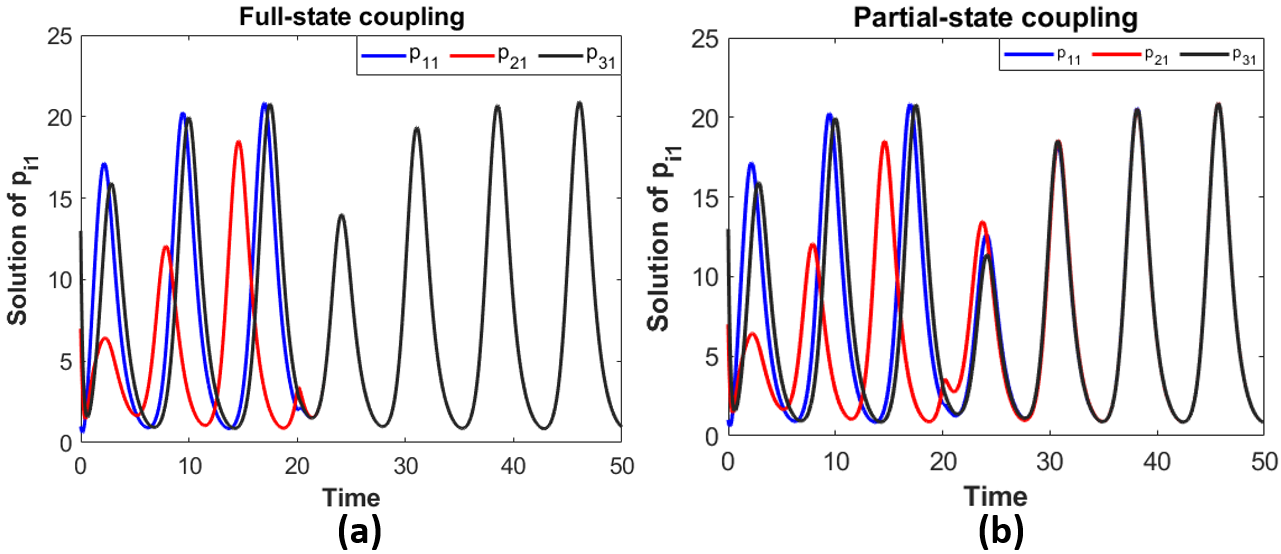
Figure 3: Numerical simulation of three coupled repressilator for different parameters value $\alpha=1000$, $\alpha_{0}=1$, $\beta=5$, $n=2$, $\text{initial condition:}(p_{10}=[0,1,0,3,0,5],p_{20}=[0,7,0,9,0,11],p_{30}=[0,13,15,17,4,6])$ and $K=1$. (a) Synchronization with full-state coupling (b) Synchronization with partial-state coupling.

V Experimental Results

To complement the numerical simulations, an electronic testbed was designed to investigate the synchronization behaviour of nonlinear oscillators.

Symbol	Parameter	Value	Units
$R_{i}$	resistor	$1.0\pm 5\%$	$K\Omega$
$R_{j}$	resistor	$1.0\pm 5\%$	$M\Omega$
$C_{i}$	capacitor	$1.0\pm 10\%$	$\mu F$
op-amp	UA741CN
Potentiometer	variable resistor	$100.0\pm 5\%$	$K\Omega$
$V_{1}$ and $V_{2}$	voltage source	$\pm 12$	V
Analog multiplier	AD633JNZ

TABLE I: Electronic components in the experiment

Example 1: Van der Pol oscillator. The oscillator circuit was realized using operational amplifiers, analog multipliers, resistors, and capacitors [32]. Op-amps introduce nonlinearities, while analog multipliers capture the quadratic terms in the Van der Pol equation. Resistors and capacitors are used to tune the time constants and obtain the oscillator behavior. The electronic circuit of the Van der Pol oscillator is given in Fig. 4.

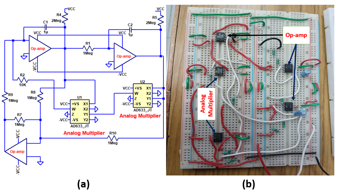
Figure 4: Circuit diagram of a Van der Pol oscillator. (a) LT Spice design, (b) experimental implementation.

We investigated the synchronization behavior of three identical Van der Pol oscillators connected in all-to-all topology. The LT Spice simulation, using the components value listed in Table 1, is shown in Fig. 5(a). As depicted in the figure, the Van der Pol oscillators exhibited independent oscillations between $0-50$ sec. After $50$ sec, the coupling is turned on, and all three oscillators get synchronized (Fig. 5(a)).

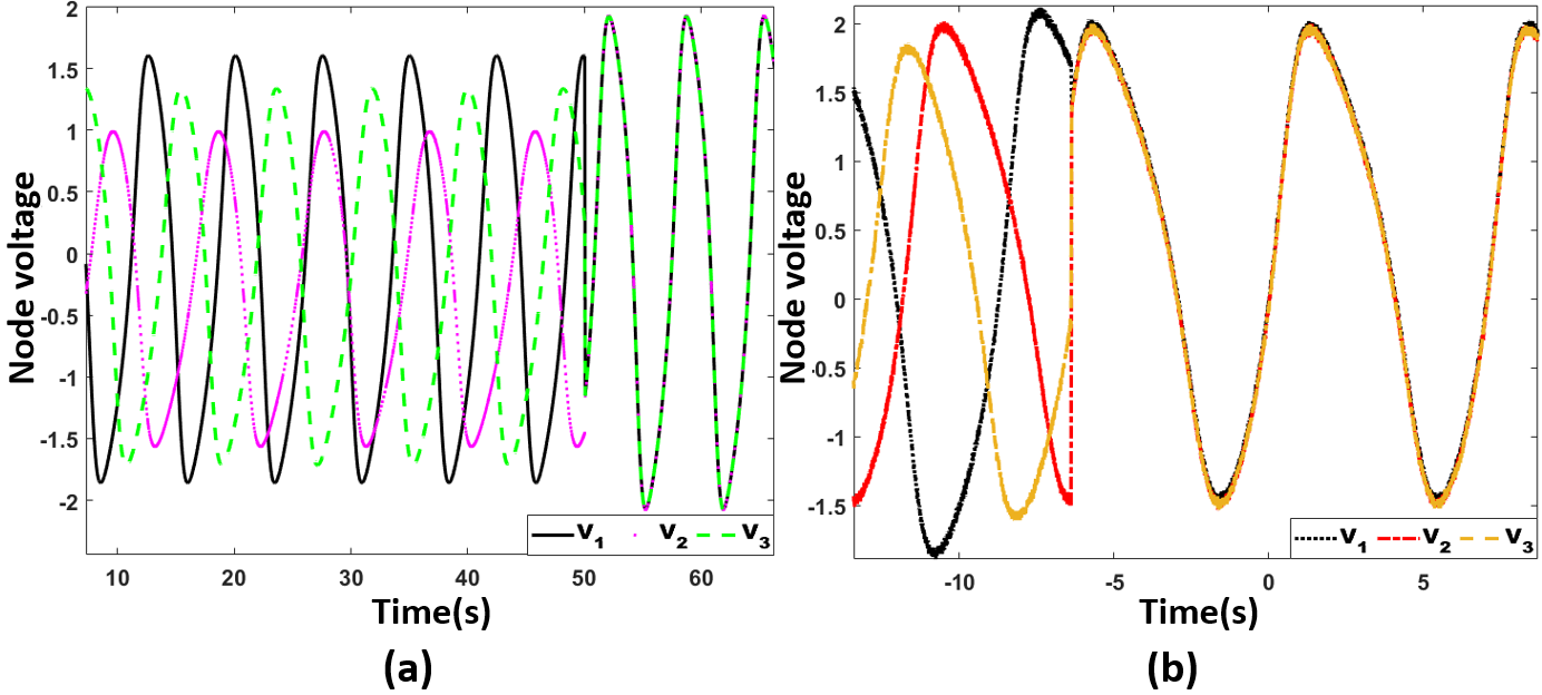
Figure 5: Synchronization of three Van der Pol oscillators coupled with different physical parameters is given in Table 1. (a) LT Spice simulation and (b) experiment.

Similar behavior was observed experimentally (Fig. 5(b)), where the coupling gain was set by varying a potentiometer.

Example 2: Repressilator. Each oscillator was implemented using three op-amps, resistors, and capacitors in a negative feedback ring topology (Fig. 6) [13, 14]. The nonlinear sigmoidal [33] characteristic of the op-amp was well suited to the nonlinearity in the repressilator equations. The output voltage of each of the op-amps was analogous to protein concentration. A resistor-capacitor network was used to implement the integration. The component values and biasing voltages are listed in Table 1.

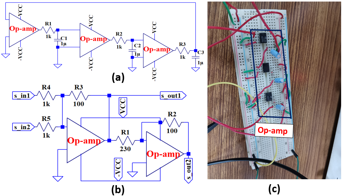
Figure 6: Circuit diagram of repressilator. (a) LT Spice design, (b) coupling circuit, (c) experimental implementation

We found that the circuit exhibited oscillations in the LT Spice simulations. As the output voltage of node two ($V_{2}$) increases, it results in the reduction of the output voltage $V_{3}$. This is because of the influence at the inverting input of the corresponding op-amps and the crossing of the threshold voltage, which is $0$ V. Similarly, as $V_{3}$ decreases, $V_{1}$ will increase, which in turn will decrease $V_{2}$. This process leads to oscillatory behavior. The phase difference between successive nodes was 120 ^∘, as expected for a 3-node ring oscillator. All three repressilators were connected in an all-to-all topology and were synchronized once the coupling was activated at $t=0.034$ sec (Fig. 7(a)). Before the coupling was activated, all the oscillators were oscillating independently (Fig. 7(a)). Similar behaviour was observed experimentally (Fig. 7(b)), where the coupling gain was set by varying a potentiometer.

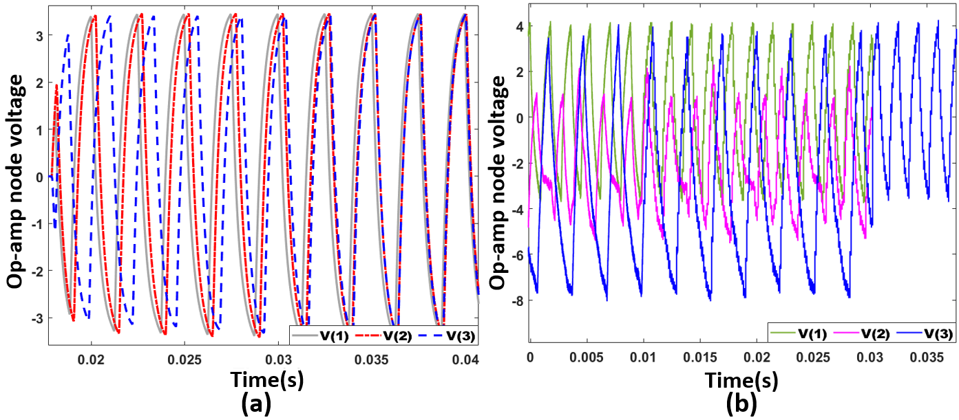
Figure 7: Synchronization of three coupled repressilators with different physical parameters is given in Table 1. (a) LT Spice simulation and (b) experiment.

VI Conclusion

We proved a necessary and sufficient condition for synchronizing a network of identical oscillators coupled linearly and in a full-state fashion. The derived condition is that the coupling constant is positive. These conditions are derived using the Lyapunov-Floquet theory and the Master Stability Function approach. Moreover, in the case of partial state coupling, a positive coupling constant ensures that the volume in the state space converges to zero asymptotically. Numerical computation of the Master Stability Function for a second-order oscillator showed that a positive coupling ensures synchronization. These results are illustrated on benchmark oscillators using numerical simulations, LT SPICE, and electronic implementation.

References

- [1] S. Strogatz, “Sync: The emerging science of spontaneous order,” 2004.
- [2] A. Pikovsky, J. Kurths, M. Rosenblum, and J. Kurths, Synchronization: a universal concept in nonlinear sciences. No. 12, Cambridge university press, 2003.
- [3] B. Ermentrout, “An adaptive model for synchrony in the firefly pteroptyx malaccae,” Journal of Mathematical Biology, vol. 29, no. 6, pp. 571–585, 1991.
- [4] S. H. Strogatz, “Nonlinear dynamics and chaos,” 1996.
- [5] E. M. Izhikevich, Dynamical systems in neuroscience. MIT press, 2007.
- [6] C. D. Brody and J. Hopfield, “Simple networks for spike-timing-based computation, with application to olfactory processing,” Neuron, vol. 37, no. 5, pp. 843–852, 2003.
- [7] N. Kopell, “We got rhythm: Dynamical systems of the nervous system,” Notices of the AMS, vol. 47, no. 1, pp. 6–16, 2000.
- [8] W. Singer, “Neuronal synchrony: a versatile code for the definition of relations?,” Neuron, vol. 24, no. 1, pp. 49–65, 1999.
- [9] T. L. Carroll and L. M. Pecora, “Synchronizing nonautonomous chaotic circuits,” IEEE Transactions on Circuits and Systems II: Analog and Digital Signal Processing, vol. 40, no. 10, pp. 646–650, 1993.
- [10] Y. Tang, A. Mees, and L. Chua, “Synchronization and chaos,” IEEE Transactions on Circuits and Systems, vol. 30, no. 9, pp. 620–626, 1983.
- [11] C. W. Wu and L. O. Chua, “Synchronization in an array of linearly coupled dynamical systems,” IEEE Transactions on Circuits and Systems I: Fundamental Theory and Applications, vol. 42, no. 8, pp. 430–447, 1995.
- [12] Z. Liu, J. Ma, G. Zhang, and Y. Zhang, “Synchronization control between two Chua’s circuits via capacitive coupling,” Applied Mathematics and Computation, vol. 360, pp. 94–106, 2019.
- [13] J. M. Buldú, J. García-Ojalvo, A. Wagemakers, and M. A. Sanjuán, “Electronic design of synthetic genetic networks,” International Journal of Bifurcation and Chaos, vol. 17, no. 10, pp. 3507–3511, 2007.
- [14] S. Y. Shafi, M. Arcak, M. Jovanović, and A. K. Packard, “Synchronization of diffusively-coupled limit cycle oscillators,” Automatica, vol. 49, no. 12, pp. 3613–3622, 2013.
- [15] L. M. Pecora and T. L. Carroll, “Master stability functions for synchronized coupled systems,” Physical Review Letters, vol. 80, no. 10, pp. 2109–2112, 1998.
- [16] W. Wang and J.-J. E. Slotine, “On partial contraction analysis for coupled nonlinear oscillators,” Biological cybernetics, vol. 92, no. 1, pp. 38–53, 2005.
- [17] G. Russo and J. J. E. Slotine, “Global convergence of quorum-sensing networks,” Physical Review E, vol. 82, no. 4, p. 041919, 2010.
- [18] L. Scardovi and R. Sepulchre, “Synchronization in networks of identical linear systems,” in 47th Conference on Decision and Control (CDC), pp. 546–551, IEEE, 2008.
- [19] M. Barahona and L. M. Pecora, “Synchronization in small-world systems,” Physical review letters, vol. 89, no. 5, p. 054101, 2002.
- [20] H. Gu, K. Liu, and J. Lü, “Adaptive pi control for synchronization of complex networks with stochastic coupling and nonlinear dynamics,” IEEE Transactions on Circuits and Systems I: Regular Papers, vol. 67, no. 12, pp. 5268–5280, 2020.
- [21] A. Jadbabaie, N. Motee, and M. Barahona, “On the stability of the kuramoto model of coupled nonlinear oscillators,” in Proceedings of the 2004 American Control Conference, vol. 5, pp. 4296–4301, IEEE, 2004.
- [22] E. N. Davison, B. Dey, and N. E. Leonard, “Synchronization bound for networks of nonlinear oscillators,” in 54th Annual Allerton Conference on Communication, Control, and Computing (Allerton), pp. 1110–1115, IEEE, 2016.
- [23] S. K. Joshi, S. Sen, and I. N. Kar, “Synchronization of coupled benchmark oscillators: analysis and experiments,” International Journal of Dynamics and Control, vol. 10, no. 2, pp. 577–597, 2022.
- [24] A. Wagemakers, J. M. Buldú, J. García-Ojalvo, and M. A. Sanjuán, “Synchronization of electronic genetic networks,” Chaos: An Interdisciplinary Journal of Nonlinear Science, vol. 16, no. 1, p. 013127, 2006.
- [25] M. Lodi, M. Forti, and M. Storace, “Stability analysis of the synchronous solution in arrays of memristive Chua’s circuits,” IEEE Transactions on Circuits and Systems II: Express Briefs, no. 5, pp. 1694–1698, 2023.
- [26] V. A. Yakubovich and V. M. Starzhinskii, Linear differential equations with periodic coefficients. New York: Wiley, 1975.
- [27] S. Sinha, R. Pandiyan, and J. Bibb, “Liapunov-floquet transformation: Computation and applications to periodic systems,” Journal of Vibration and Acoustics, vol. 118, pp. 209–219, 1996.
- [28] R. W. Brockett, Finite dimensional linear systems. SIAM, 2015.
- [29] M. B. Elowitz and S. Leibler, “A synthetic oscillatory network of transcriptional regulators,” Nature, vol. 403, no. 6767, pp. 335–338, 2000.
- [30] E. H. Hellen, E. Volkov, J. Kurths, and S. K. Dana, “An electronic analog of synthetic genetic networks,” PLoS One, vol. 6, no. 8, p. e23286, 2011.
- [31] E. H. Hellen, S. K. Dana, B. Zhurov, and E. Volkov, “Electronic implementation of a repressilator with quorum sensing feedback,” PLoS One, vol. 8, no. 5, p. e62997, 2013.
- [32] J. K. Roberge, Operational amplifiers: theory and practice, vol. 197. Wiley New York, 1975.
- [33] R. Gesztelyi, J. Zsuga, A. Kemeny-Beke, B. Varga, B. Juhasz, and A. Tosaki, “The hill equation and the origin of quantitative pharmacology,” Archive for history of exact sciences, vol. 66, no. 4, pp. 427–438, 2012.