Best-in-class modeling:
A novel strategy to discover constitutive models for soft matter systems

Abstract

The ability to automatically discover interpretable mathematical models from data could forever change how we model soft matter systems. For convex discovery problems with a unique global minimum, model discovery is well-established. It uses a classical top-down approach that first calculates a dense parameter vector, and then sparsifies the vector by gradually removing terms. For non-convex discovery problems with multiple local minima, this strategy is infeasible since the initial parameter vector is generally non-unique. Here we propose a novel bottom-up approach that starts with a sparse single-term vector, and then densifies the vector by systematically adding terms. Along the way, we discover models of gradually increasing complexity, a strategy that we call best-in-class modeling. To identify and select successful candidate terms, we reverse-engineer a library of sixteen functional building blocks that integrate a century of knowledge in material modeling with recent trends in machine learning and artificial intelligence. Yet, instead of solving the NP hard discrete combinatorial problem with $2^{16}=65,536$ possible combinations of terms, best-in-class modeling starts with the best one-term model and iteratively repeats adding terms, until the objective function meets a user-defined convergence criterion. Strikingly, for most practical purposes, we achieve good convergence with only one or two terms. We illustrate the best-in-class one- and two-term models for a variety of soft matter systems including rubber, brain, artificial meat, skin, and arteries. Our discovered models display distinct and unexpected features for each family of materials, and suggest that best-in-class modeling is an efficient, robust, and easy-to-use strategy to discover the mechanical signatures of traditional and unconventional soft materials. We anticipate that our technology will generalize naturally to other classes of natural and man made soft matter with applications in artificial organs, stretchable electronics, soft robotics, and artificial meat.

1 Motivation

Exactly 200 years ago, Augustin-Louis Cauchy formalized the concept of stress [8]. Ever since then, research in mechanics has focused on discovering mathematical models that map strains onto stresses [42]. As we now know, this is by no means trivial. In fact, for more almost a century, the limiting roadblock between experiments and simulation has been the process of material modeling [19]: Material modeling is limited to expert specialists, prone to user bias, and vulnerable to human error. Yet, today, as we are discovering new soft materials at an unprecedented rate, material modeling has become more important than ever. Soft materials are emerging everywhere, in artificial organs, wearable devices, stretchable electronics, soft robotics, smart textiles, and even in artificial meat. This creates a unique opportunity: What if we could take the human out of the loop and automate the process of model discovery?
Automating model discovery is precisely what this manuscript is about. We propose a novel technology that leverages recent developments in artificial intelligence [27], machine learning [2], and constitutive neural networks [30] to autonomously discover the best model and parameters to describe soft matter systems. Our approach builds on recent developments to systematically learn stresses from strains using neural networks [14, 25, 52]. However, rather than using generic off-the-shelf network architectures, we embrace a recent trend in the mechanics community to develop our own constitutive neural networks that satisfy physical restrictions and thermodynamic constraints [29, 31]. While most of these approaches focus on finding the best-fit model regardless of model complexity [3, 53], our goal is to discover models that not only explain given data, but are also interpretable and generalizable by design [6, 11, 32]. Practically speaking, the models we seek to discover need to be sparse.
Sparse regression is a special type of regression that prevents overfitting by training a large number of parameters to zero [54]. This is especially useful in high-dimensional settings, where it generates simple interpretable models with a small subset of non-zero parameters [13]. Sparse regression translates model discovery into a discrete subset selection or feature extraction task that is known in statistics as $L_{0}$ regularization [12]. In the context of linear regression, subset selection has become standard textbook knowledge [18]. In the context of nonlinear regression, when analytical solutions are rare, subset selection is much more nuanced, general recommendations are difficult, and feature extraction becomes highly problem-specific [24]. To be clear, this limitation is not exclusively inherent to automated model discovery with constitutive neural networks; it applies to distilling scientific knowledge from data in general [46]. In fluid mechanics, a typical example is turbulence modeling, where we seek to approximate intricate interactions between different scales that can be well represented through polynomials [5]. In solid mechanics, we seek to approximate complex material behaviors at the microscopic scale through a combination of polynomials [17], exponentials [9, 21], logarithms [16], and powers [41, 58]. In the context of model discovery, polynomial models translate into a convex linear optimization problem with a single unique global minimum, while exponential, logarithmic, or power models translate into a non-convex nonlinear optimization problem with possibly multiple local minima [36]. This raises the question how do we robustly discover interpretable and generalizable constitutive models from data?

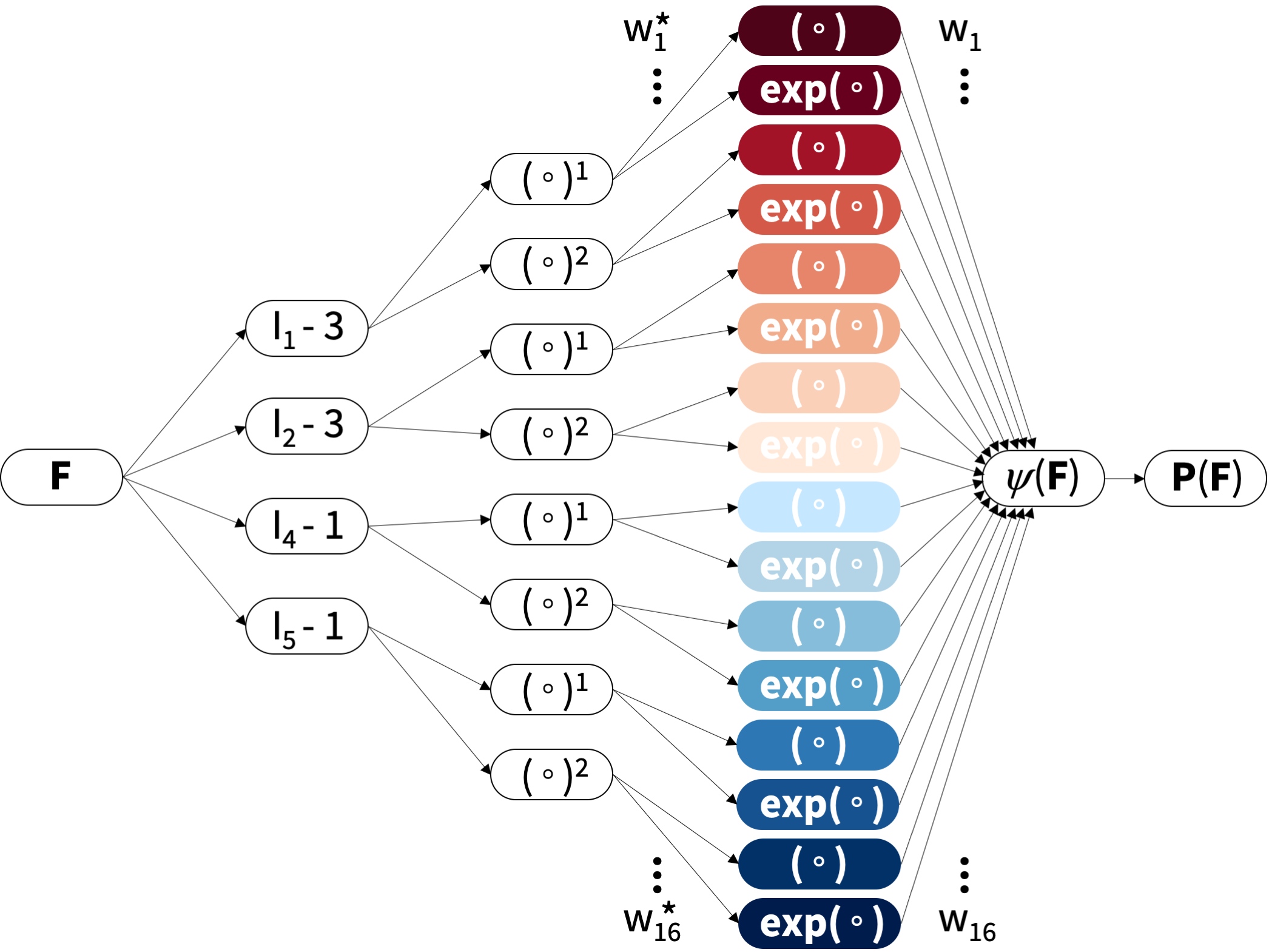
Figure 1: Constitutive neural network for best-in-class modeling. The network takes the deformation gradient $F$ as input and outputs the free energy function $\psi$ from which we calculate the stress $\mbox{\boldmath$P$}{}=\partial\psi/\partial\mbox{\boldmath$F$}{}$. The network first calculates functions of four invariants $[I_{1}-3],[I_{2}-3],[I_{4}-1],[I_{5}-1]]$ and feeds them into its two hidden layers. The first layer generates the first and second powers $(\circ)$ and $(\circ)^{2}$ of the invariants and the second layer applies the identity and exponential function $(\circ)$ and $\exp(\circ)$ to these powers multiplied by the weights $\mbox{\boldmath$w$}{}^{*}=[w_{1}^{*},...w_{16}^{*}]$. The free energy function $\psi$ is the sum of these sixteen color-coded terms, multiplied by the weights $\mbox{\boldmath$w$}{}=[w_{1},...w_{16}]$. Red terms associated with the weights $w_{1},...,w_{8}$ are isotropic terms; blue terms associated with the weights $w_{9},...,w_{16}$ are anisotropic terms. We train the network by minimizing the error between model $\mbox{\boldmath$P$}{}(\mbox{\boldmath$F$}{},\mbox{\boldmath$w$}{},\mbox{\boldmath$w$}{}^{*})$ and data $\hat{\mbox{\boldmath$P$}{}}$ to learn the network parameters $w$ and $\mbox{\boldmath$w$}{}^{*}$, and apply L₀ regularization to sparsify the parameter vector $w$.

Two competing strategies have emerged to discover interpretable mathematical models: sparsification and densification. For convex discovery problems with a unique global minimum, sparsification has been well established through a top-down approach [5, 10]. It first calculates a dense parameter vector at the global minimum, and then sparsifies the parameter vector by sequential thresholding, and removes the least relevant terms [59, 60]. For non-convex discovery problems with multiple local minima, this strategy is infeasible since different initial conditions may result in non-unique initial parameter vectors [42]. Instead of trying to sparsify an initially dense parameter vector, it seems reasonable to gradually densify an initially sparse parameter vector from scratch [40]. This bottom-up approach iteratively solves a sequence of discrete combinatorial problems, and densifies the parameter vector by sequentially adding the most relevant terms [36]. Importantly, instead of solving the NP hard discrete combinatorial problem associated with screening all possible combinations of terms [26], we gradually add terms, starting with the best-in-class one-term model, and iteratively repeat adding terms, until the overall loss function meets a user-defined convergence criterion. For most practical purposes, it is sufficient to limit the number of desirable terms to one, two, or three, and identify the best-in-class model of each class. The objective of this manuscript is to establish the concept of best-in-class modeling and discover the best one- and two-term models for five distinct soft matter systems: rubber, brain, artificial meat, skin, and arteries.

2 Continuum mechanics

Kinematics. Throughout this manuscript, we illustrate best-in-class model discovery for mechanical test data from tension, compression, and shear tests. During mechanical testing [57], particles $X$ of the undeformed sample map to particles $\mbox{\boldmath$x$}{}=\mbox{\boldmath$\varphi$}{}(\mbox{\boldmath$X$}{})$ of the deformed sample via the deformation map $\varphi$. Its gradient with respect to the undeformed coordinates $X$ is the deformation gradient $F$ with Jacobian $J$,

$$\mbox{\boldmath$F$}{}=\nabla_{\bm{X}}\mbox{\boldmath$\varphi$}{}\quad\mbox{and}\quad J=\det(\mbox{\boldmath$F$}{})\,.$$ (1)

Here we consider perfectly incompressible materials with a constant Jacobian $J=1$, and transversely isotropic materials with one pronounced direction $\mbox{\boldmath$n$}{}_{0}$. The undeformed direction vector has a unit length, $||\,\mbox{\boldmath$n$}{}_{0}\,||=1$, and maps onto the deformed direction vector, $\mbox{\boldmath$n$}{}=\mbox{\boldmath$F$}{}\cdot\mbox{\boldmath$n$}{}_{0}$, with a stretch, $||\,\mbox{\boldmath$n$}{}\,||=\lambda_{\rm{n}}$. We characterize the deformation state of the sample through the two isotropic invariants $I_{1}$ and $I_{2}$ and two anisotropic invariants $I_{4}$ and $I_{5}$ [47],

$$\begin{array}[]{r@{\hspace*{0.05cm}}c@{\hspace*{0.10cm}} r@{\hspace*{0.05cm}}c@{\hspace*{0.05cm}} l@{\hspace*{0.50cm}}l@{\hspace*{0.05cm}} c@{\hspace*{0.10cm}}r@{\hspace*{0.05cm}} c@{\hspace*{0.05cm}}l@{\hspace*{-0.1cm}}}I_{1}\hskip 1.42271pt&=\hfil\hskip 2.84544pt&[\hskip 1.42271pt&\mbox{\boldmath$F$}{}^{\mbox{{\scriptsize{${\rm{t}}$}}}{}}\cdot\mbox{\boldmath$F$}{}\hfil\hskip 1.42271pt&]:\mbox{\boldmath$I$}{}\hfil\hskip 14.22636pt&I_{2}\hfil\hskip 1.42271pt&=\hfil\hskip 2.84544pt&\frac{1}{2}\;[I_{1}^{2}-[\hskip 1.42271pt&\mbox{\boldmath$F$}{}^{\mbox{{\scriptsize{${\rm{t}}$}}}{}}\cdot\mbox{\boldmath$F$}{}\hfil\hskip 1.42271pt&]:[\,\mbox{\boldmath$F$}{}^{\mbox{{\scriptsize{${\rm{t}}$}}}{}}\cdot\mbox{\boldmath$F$}{}\,]]\\ I_{4}\hskip 1.42271pt&=\hfil\hskip 2.84544pt&\mbox{\boldmath$n$}{}_{0}\cdot[\hskip 1.42271pt&\mbox{\boldmath$F$}{}^{\mbox{{\scriptsize{${\rm{t}}$}}}{}}\cdot\mbox{\boldmath$F$}{}\hfil\hskip 1.42271pt&]\cdot\mbox{\boldmath$n$}{}_{0}\hfil\hskip 14.22636pt&I_{5}\hfil\hskip 1.42271pt&=\hfil\hskip 2.84544pt&\mbox{\boldmath$n$}{}_{0}\cdot[\hskip 1.42271pt&\mbox{\boldmath$F$}{}^{\mbox{{\scriptsize{${\rm{t}}$}}}{}}\cdot\mbox{\boldmath$F$}{}\hfil\hskip 1.42271pt&]^{2}\!\cdot\mbox{\boldmath$n$}{}_{0}\,,\end{array}$$ (2)

and note that the third invariant is constant, $I_{3}=J^{2}=1$, and the fourth invariant is the stretch of the direction vector squared, $I_{4}=\lambda_{\rm{n}}^{2}$.
Constitutive equations. We reverse-engineer a free energy function for perfectly incompressible, transversely isotropic, hyperelastic materials as a function of these four invariants $[I_{1}-3]$, $[I_{2}-3]$, $[I_{4}-1]$, $[I_{5}-1]$, raised to the first and second powers, $(\circ)^{1}$ and $(\circ)^{2}$, embedded into the identity $(\circ)$ and the exponential function $(\rm{exp}(\circ)-1)$ [31]. Figure 1 illustrates how the weighted sum of all sixteen terms defines the strain energy function $\psi(\mbox{\boldmath$F$}{})$ [33],

$$\begin{array}[]{l@{\hspace*{.10cm}}c@{\hspace*{.10cm}} l@{\hspace*{.05cm}}l@{\hspace*{.05cm}} l@{\hspace*{.10cm}}l@{\hspace*{.05cm}} l@{\hspace*{.10cm}}l@{\hspace*{.00cm}}l}\psi\hfil\hskip 2.84544pt&=\hfil\hskip 2.84544pt&w_{1}\hfil\hskip 1.42271pt&[I_{1}-3]\hfil\hskip 1.42271pt&+\hfil\hskip 2.84544pt&w_{2}\hfil\hskip 1.42271pt&[\,\exp(w^{*}_{2}\hfil\hskip 2.84544pt&[I_{1}-3]&)-1]\\ \hfil\hskip 2.84544pt&+\hfil\hskip 2.84544pt&w_{3}\hfil\hskip 1.42271pt&[I_{1}-3]^{2}\hfil\hskip 1.42271pt&+\hfil\hskip 2.84544pt&w_{4}\hfil\hskip 1.42271pt&[\,\exp(w^{*}_{4}\hfil\hskip 2.84544pt&[I_{1}-3]^{2}&)-1]\\ \hfil\hskip 2.84544pt&+\hfil\hskip 2.84544pt&w_{5}\hfil\hskip 1.42271pt&[I_{2}-3]\hfil\hskip 1.42271pt&+\hfil\hskip 2.84544pt&w_{6}\hfil\hskip 1.42271pt&[\,\exp(w^{*}_{6}\hfil\hskip 2.84544pt&[I_{2}-3]&)-1]\\ \hfil\hskip 2.84544pt&+\hfil\hskip 2.84544pt&w_{7}\hfil\hskip 1.42271pt&[I_{2}-3]^{2}\hfil\hskip 1.42271pt&+\hfil\hskip 2.84544pt&w_{8}\hfil\hskip 1.42271pt&[\,\exp(w^{*}_{8}\hfil\hskip 2.84544pt&[I_{2}-3]^{2}&)-1]\\ \hfil\hskip 2.84544pt&+\hfil\hskip 2.84544pt&w_{9}\hfil\hskip 1.42271pt&[I_{4}-1]\hfil\hskip 1.42271pt&+\hfil\hskip 2.84544pt&w_{10}\hfil\hskip 1.42271pt&[\,\exp(w^{*}_{10}\hfil\hskip 2.84544pt&[I_{4}-1]&)-1]\\ \hfil\hskip 2.84544pt&+\hfil\hskip 2.84544pt&w_{11}\hfil\hskip 1.42271pt&[I_{4}-1]^{2}\hfil\hskip 1.42271pt&+\hfil\hskip 2.84544pt&w_{12}\hfil\hskip 1.42271pt&[\,\exp(w^{*}_{12}\hfil\hskip 2.84544pt&[I_{4}-1]^{2}&)-1]\\ \hfil\hskip 2.84544pt&+\hfil\hskip 2.84544pt&w_{13}\hfil\hskip 1.42271pt&[I_{5}-1]\hfil\hskip 1.42271pt&+\hfil\hskip 2.84544pt&w_{14}\hfil\hskip 1.42271pt&[\,\exp(w^{*}_{14}\hfil\hskip 2.84544pt&[I_{5}-1]&)-1]\\ \hfil\hskip 2.84544pt&+\hfil\hskip 2.84544pt&w_{15}\hfil\hskip 1.42271pt&[I_{5}-1]^{2}\hfil\hskip 1.42271pt&+\hfil\hskip 2.84544pt&w_{16}\hfil\hskip 1.42271pt&[\,\exp(w^{*}_{16}\hfil\hskip 2.84544pt&[I_{5}-1]^{2}&)-1]\,,\end{array}$$ (3)

To satisfy perfect incompressibility, we correct the free energy function by the pressure term, $\psi^{*}=-p\,[J-1]$, where $p$ is the hydrostatic pressure that we determine from the boundary conditions. We consider hyperelastic materials that satisfy the second law of thermodynamics. Their Piola stress $\mbox{\boldmath$P$}{}=\partial\psi(\mbox{\boldmath$F$}{})/\partial\mbox{\boldmath$F$}{}$ is the derivative of the free energy $\psi(\mbox{\boldmath$F$}{})$ with respect to the deformation gradient $F$,

$$\mbox{\boldmath$P$}{}=\frac{\partial\psi}{\partial\bm{F}}-p\,\bm{F}^{\text{-t}}\,.$$ (4)

This results in the following explicit representation of the Piola stress [20],

$$\mbox{\boldmath$P$}{}=\displaystyle{\frac{\partial\psi}{\partial I_{1}}\frac{\partial I_{1}}{\partial\mbox{\boldmath$F$}{}}}+\displaystyle{\frac{\partial\psi}{\partial I_{2}}\frac{\partial I_{2}}{\partial\mbox{\boldmath$F$}{}}}+\displaystyle{\frac{\partial\psi}{\partial I_{4}}\frac{\partial I_{4}}{\partial\mbox{\boldmath$F$}{}}}+\displaystyle{\frac{\partial\psi}{\partial I_{5}}\frac{\partial I_{5}}{\partial\mbox{\boldmath$F$}{}}}-\displaystyle{p\,\mbox{\boldmath$F$}{}^{-{\mbox{{\scriptsize{${\rm{t}}$}}}{}}}}\,.$$ (5)

with the following explicit expressions of the derivatives with respect to the four invariants [33],

$$\begin{array}[]{l@{\hspace*{0.10cm}}l@{\hspace*{0.1cm}} l@{\hspace*{0.04cm}}l@{\hspace*{0.0cm}} l@{\hspace*{0.04cm}}l@{\hspace*{0.1cm}} l@{\hspace*{0.10cm}}l@{\hspace*{0.1cm}} l@{\hspace*{0.04cm}}l@{\hspace*{0.0cm}}l}\displaystyle{\frac{\partial\psi}{\partial I_{1}}}\hfil\hskip 2.84544pt&=\hfil\hskip 2.84544pt&\hfil\hskip 1.13791pt&w_{1}&\hfil\hskip 1.13791pt&+\hfil\hskip 2.84544pt&w_{2}\hfil\hskip 2.84544pt&w^{*}_{2}\hfil\hskip 2.84544pt&\exp(w^{*}_{2}\hfil\hskip 1.13791pt&[I_{1}-3]&)\\[-4.0pt] \hfil\hskip 2.84544pt&+\hfil\hskip 2.84544pt&2\,[I_{1}-3][\hfil\hskip 1.13791pt&w_{3}&\hfil\hskip 1.13791pt&+\hfil\hskip 2.84544pt&w_{4}\hfil\hskip 2.84544pt&w^{*}_{4}\hfil\hskip 2.84544pt&\exp(w^{*}_{4}\hfil\hskip 1.13791pt&[I_{1}-3]^{2}&)]\\[-4.0pt] \displaystyle{\frac{\partial\psi}{\partial I_{2}}}\hfil\hskip 2.84544pt&=\hfil\hskip 2.84544pt&\hfil\hskip 1.13791pt&w_{5}&\hfil\hskip 1.13791pt&+\hfil\hskip 2.84544pt&w_{6}\hfil\hskip 2.84544pt&w^{*}_{6}\hfil\hskip 2.84544pt&\exp(w^{*}_{6}\hfil\hskip 1.13791pt&[I_{2}-3]&)\\[-4.0pt] \hfil\hskip 2.84544pt&+\hfil\hskip 2.84544pt&2\,[I_{2}-3][\hfil\hskip 1.13791pt&w_{7}&\hfil\hskip 1.13791pt&+\hfil\hskip 2.84544pt&w_{8}\hfil\hskip 2.84544pt&w^{*}_{8}\hfil\hskip 2.84544pt&\exp(w^{*}_{8}\hfil\hskip 1.13791pt&[I_{2}-3]^{2}&)]\\[-4.0pt] \displaystyle{\frac{\partial\psi}{\partial I_{4}}}\hfil\hskip 2.84544pt&=\hfil\hskip 2.84544pt&\hfil\hskip 1.13791pt&w_{9}&\hfil\hskip 1.13791pt&+\hfil\hskip 2.84544pt&w_{10}\hfil\hskip 2.84544pt&w^{*}_{10}\hfil\hskip 2.84544pt&\exp(w^{*}_{10}\hfil\hskip 1.13791pt&[I_{4}-1]&)\\[-4.0pt] \hfil\hskip 2.84544pt&+\hfil\hskip 2.84544pt&2\,[I_{4}-1][\hfil\hskip 1.13791pt&w_{11}&\hfil\hskip 1.13791pt&+\hfil\hskip 2.84544pt&w_{12}\hfil\hskip 2.84544pt&w^{*}_{12}\hfil\hskip 2.84544pt&\exp(w^{*}_{12}\hfil\hskip 1.13791pt&[I_{4}-1]^{2}&)]\\[-4.0pt] \displaystyle{\frac{\partial\psi}{\partial I_{5}}}\hfil\hskip 2.84544pt&=\hfil\hskip 2.84544pt&\hfil\hskip 1.13791pt&w_{13}&\hfil\hskip 1.13791pt&+\hfil\hskip 2.84544pt&w_{14}\hfil\hskip 2.84544pt&w^{*}_{14}\hfil\hskip 2.84544pt&\exp(\,w^{*}_{14}\hfil\hskip 1.13791pt&[I_{5}-1]&)\\[-4.0pt] \hfil\hskip 2.84544pt&+\hfil\hskip 2.84544pt&2\,[I_{5}-1][\hfil\hskip 1.13791pt&w_{15}&\hfil\hskip 1.13791pt&+\hfil\hskip 2.84544pt&w_{16}\hfil\hskip 2.84544pt&w^{*}_{16}\hfil\hskip 2.84544pt&\exp(\,w^{*}_{16}\hfil\hskip 1.13791pt&[I_{5}-1]^{2}&)].\end{array}$$ (6)

Our model contains 24 model parameters in total, sixteen with the unit of stiffness, $\mbox{\boldmath$w$}{}=[w_{1},w_{2},w_{3},w_{4},w_{5},w_{6},w_{7},w_{8},$ $w_{9},w_{10},w_{11},w_{12},w_{13},w_{14},w_{15},w_{16}]$, and eight unit-less, $\mbox{\boldmath$w$}{}^{*}=[1,w_{2}^{*},1,w^{*}_{4},1,w^{*}_{6},1,w^{*}_{8},1,w^{*}_{10},1,w^{*}_{12},1,w^{*}_{14},1,w^{*}_{16}]$, where all eight odd unit-less weights are constant and equal to one. To comply with physical constraints, we constrain all parameters to always remain non-negative, $\mbox{\boldmath$w$}{}\geq\mbox{\boldmath$0$}{}$ and $\mbox{\boldmath$w$}{}^{*}\geq\mbox{\boldmath$0$}{}$.

3 Data

We consider data from homogeneous uniaxial tension and compression, simple shear, pure shear, equibiaxial extension, and biaxial extension tests on vulcanized rubber [55], human brain gray and white matter [7], artificial meat tofurkey [49], porcine skin [33], and human aortic media and adventitia [44].
Uniaxial tension and compression. For the case of uniaxial tension and compression, with a stretch $\lambda$ in the $\{1,1\}$-direction, such that $\mbox{\boldmath$F$}{}=\mbox{diag}\,\{\,\lambda,\lambda^{-1/2},\lambda^{-1/2}\,\}$ and $\mbox{\boldmath$P$}{}=\mbox{diag}\,\{\,P_{11},0,0\,\}$, the stress-stretch relation for isotropic materials [32] is

$$P_{11}=2\,\left[\frac{\partial\psi}{\partial I_{1}}+\frac{1}{\lambda}\frac{\partial\psi}{\partial I_{2}}\right]\left[\lambda-\frac{1}{\lambda^{2}}\right]\,.$$ (7)

Simple shear. For the case of simple shear, with a shear $\gamma$ in the $\{1,2\}$-direction, such that $F_{12}=\gamma$, the shear stress-strain relation for isotropic materials [32] is

$$P_{12}=2\,\left[\frac{\partial\psi}{\partial I_{1}}+\frac{\partial\psi}{\partial I_{2}}\right]\gamma\,.$$ (8)

Pure shear. For the case of pure shear of a long rectangular specimen stretched with $\lambda$ along its short axis in the $\{1,1\}$-direction, and no deformation along it long axis in the $\{2,2\}$-direction, such that $\mbox{\boldmath$F$}{}=\mbox{diag}\,\{\,\lambda,1,\lambda^{-1}\,\}$ and $\mbox{\boldmath$P$}{}=\mbox{diag}\,\{\,P_{11},P_{22},0\,\}$, the stress-stretch relations for isotropic materials [31] are

$$\begin{array}[]{c@{\hspace*{.10cm}}c@{\hspace*{.10cm}} c@{\hspace*{.05cm}}c@{\hspace*{.05cm}} c@{\hspace*{.05cm}}r@{\hspace*{.05cm}}l}P_{11}\hfil\hskip 2.84544pt&=\hfil\hskip 2.84544pt&\displaystyle{2}\hfil\hskip 1.42271pt&\displaystyle{\left[\frac{\partial\psi}{\partial I_{1}}\right.}\hfil\hskip 1.42271pt&+\hfil\hskip 1.42271pt&\displaystyle{\left.\frac{\partial\psi}{\partial I_{2}}\right]}\hskip 1.42271pt&\displaystyle{\left[\lambda-\frac{1}{\lambda^{3}}\right]}\\[12.91663pt] P_{22}\hfil\hskip 2.84544pt&=\hfil\hskip 2.84544pt&\displaystyle{2}\hfil\hskip 1.42271pt&\displaystyle{\left[\frac{\partial\psi}{\partial I_{1}}\right.}\hfil\hskip 1.42271pt&+\hfil\hskip 1.42271pt&\displaystyle{\left.\lambda^{2}\frac{\partial\psi}{\partial I_{2}}\right]}\hskip 1.42271pt&\displaystyle{\left[1-\frac{1}{\lambda^{2}}\right]}\,.\end{array}$$ (9)

Equibiaxial extension. For the case of equibiaxial extension, with a stretch $\lambda$ in the $\{1,1\}$- and $\{2,2\}$-directions, such that $\mbox{\boldmath$F$}{}=\mbox{diag}\,\{\,\lambda,\lambda,\lambda^{-2}\,\}$ and $\mbox{\boldmath$P$}{}=\mbox{diag}\,\{\,P_{11},P_{22},0\,\}$, the stress-stretch relation for isotropic materials [31] is

$$P_{11}=2\,\left[\frac{\partial\psi}{\partial I_{1}}+\lambda^{2}\frac{\partial\psi}{\partial I_{2}}\right]\left[\lambda-\frac{1}{\lambda^{5}}\right]=P_{22}\,.$$ (10)

Biaxial extension. For the case of biaxial extension, with stretches $\lambda_{1}$ and $\lambda_{2}$ in the $\{1,1\}$- and $\{2,2\}$-directions, such that $\mbox{\boldmath$F$}{}=\mbox{diag}\,\{\,\lambda_{1},\lambda_{2},(\lambda_{1}\lambda_{2})^{-1}\,\}$ and $\mbox{\boldmath$P$}{}=\mbox{diag}\,\{\,P_{11},P_{22},0\,\}$, the stress-stretch relations for transversely isotropic materials with one single fiber family [33] are

$$\begin{array}[]{ @{\hspace*{.02cm}} c@{\hspace*{.05cm}}c@{\hspace*{.05cm}} c@{\hspace*{.05cm}}c@{\hspace*{.05cm}} c@{\hspace*{.05cm}}c@{\hspace*{.05cm}} c@{\hspace*{.05cm}}c@{\hspace*{.05cm}}l}\hskip 0.56917pt\lx@intercol\hfil P_{11}\hfil\hskip 1.42271pt&=\hfil\hskip 1.42271pt&\displaystyle{2}\hfil\hskip 1.42271pt&\displaystyle{\left[\lambda_{1}-\frac{1}{\lambda_{1}^{2}\lambda_{2}^{2}}\right]}\hfil\hskip 1.42271pt&\displaystyle{\frac{\partial\psi}{\partial I_{1}}}\hfil\hskip 1.42271pt&+\hfil\hskip 1.42271pt&\displaystyle{2}\hfil\hskip 1.42271pt&\displaystyle{\left[\,\lambda_{1}\lambda_{2}^{2}+\frac{\lambda_{1}-\lambda_{1}^{2}-\lambda_{2}^{2}}{\lambda_{1}^{2}\lambda_{2}^{2}}\right]}\hfil\hskip 1.42271pt&\displaystyle{\frac{\partial\psi}{\partial I_{2}}}\\ \hskip 0.56917pt\lx@intercol\hfil\hfil\hskip 1.42271pt&+\hfil\hskip 1.42271pt&\displaystyle{2}\hfil\hskip 1.42271pt&\displaystyle{\lambda_{1}{\rm{\cos}}^{2}\alpha}\hfil\hskip 1.42271pt&\displaystyle{\frac{\partial\psi}{\partial I_{4}}}\hfil\hskip 1.42271pt&+\hfil\hskip 1.42271pt&\displaystyle{4}\hfil\hskip 1.42271pt&\displaystyle{\lambda_{1}^{3}{\rm{\cos}}^{2}\alpha}\hfil\hskip 1.42271pt&\displaystyle{\frac{\partial\psi}{\partial I_{5}}}\\[6.0pt] \hskip 0.56917pt\lx@intercol\hfil P_{22}\hfil\hskip 1.42271pt&=\hfil\hskip 1.42271pt&\displaystyle{2}\hfil\hskip 1.42271pt&\displaystyle{\left[\lambda_{2}-\frac{1}{\lambda_{1}^{2}\lambda_{2}^{2}}\right]}\hfil\hskip 1.42271pt&\displaystyle{\frac{\partial\psi}{\partial I_{1}}}\hfil\hskip 1.42271pt&+\hfil\hskip 1.42271pt&\displaystyle{2}\hfil\hskip 1.42271pt&\displaystyle{\left[\,\lambda_{1}^{2}\lambda_{2}+\frac{\lambda_{2}-\lambda_{1}^{2}-\lambda_{2}^{2}}{\lambda_{1}^{2}\lambda_{2}^{2}}\right]}\hfil\hskip 1.42271pt&\displaystyle{\frac{\partial\psi}{\partial I_{2}}}\\ \hskip 0.56917pt\lx@intercol\hfil\hfil\hskip 1.42271pt&+\hfil\hskip 1.42271pt&\displaystyle{2}\hfil\hskip 1.42271pt&\displaystyle{\lambda_{2}{\rm{sin}}^{2}\alpha}\hfil\hskip 1.42271pt&\displaystyle{\frac{\partial\psi}{\partial I_{4}}}\hfil\hskip 1.42271pt&+\hfil\hskip 1.42271pt&\displaystyle{4}\hfil\hskip 1.42271pt&\displaystyle{\lambda_{2}^{3}{\rm{\sin}}^{2}\alpha}\hfil\hskip 1.42271pt&\displaystyle{\frac{\partial\psi}{\partial I_{5}}}.\end{array}$$ (11)

The stress-stretch relations for transversely isotropic materials with two symmetric fiber families are identical to equation (11), with the $\partial\psi/\partial I_{4}$ and $\partial\psi/\partial I_{5}$ terms multiplied by an additional factor two [44]. Importantly, for both cases, one single fiber family and two symmetric fiber families, it is critical that the samples are mounted symmetrically to the stretch directions to ensure a shear-free homogeneous deformation state.

4 Best-in-class modeling

To discover the best-in-class models and parameters $w$ and $\mbox{\boldmath$w$}{}^{*}$, we minimize the loss function $L$ that penalizes the error between the discovered model and the experimental data. We characterize this error as the mean squared error, the $L_{2}$-norm of the difference between model $\mbox{\boldmath$P$}{}(\mbox{\boldmath$F$}{}_{i},\mbox{\boldmath$w$}{},\mbox{\boldmath$w$}{}^{*})$ and data $\hat{\mbox{\boldmath$P$}{}}_{i}$, divided by the number of data points $n_{\rm{data}}$. We apply $L_{0}$ regularization and supplement the loss function by the product of the $L_{0}$ norm of the parameter vector $w$, weighted by a penalty parameter $\alpha$,

$$L(\mbox{\boldmath$w$}{},\mbox{\boldmath$w$}{}^{*};\mbox{\boldmath$F$}{})=\frac{1}{n_{\rm{data}}}\!\sum_{i=1}^{n_{\rm{data}}}\!||\mbox{\boldmath$P$}{}(\mbox{\boldmath$F$}{}_{i},\mbox{\boldmath$w$}{},\mbox{\boldmath$w$}{}^{*})-\hat{\mbox{\boldmath$P$}{}}_{i}\,||^{2}+\alpha\,||\,\mbox{\boldmath$w$}{}\,||_{0}\!\rightarrow\min_{\mbox{{\boldmath{\scriptsize{$w$}}}}{}}.$$ (12)

The $L_{0}$ norm is often referred to as the sparse norm and is not a norm in a strict mathematical sense. It refers to the pseudo-norm, $||\,\mbox{\boldmath$w$}{}\,||_{0}=\sum_{i=1}^{n_{\rm{w}}}I(w_{i}\neq 0)$, where $I(\circ)$ is the indicator function that is one if the condition inside the parenthesis is true and zero otherwise. As such, the $L_{0}$ norm counts the number of non-zero entries in a vector and is an explicit switch to penalize model complexity. In the following sections, we minimize the loss function (12) to discover the best models and parameters for rubber, brain, artificial meat, skin, and arteries, report the discovered best-in-class one- and two-term models, and compare them to traditional models used in the literature.
Best-in-class rubber models. To discover the best model and parameters for rubber, we use the popular and widely studied uniaxial tension, equibiaxial tension, and pure shear experiments on vulcanized rubber [31, 55].

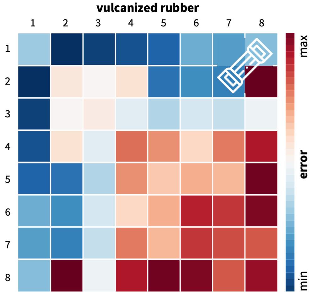
Figure 2: Best-in-class rubber models. Discovered one-term models, diagonal, and two-term models, off-diagonal, for isotropic vulcanized rubber. Models are made up of eight functional building blocks: linear, exponential linear, quadratic, and exponential quadratic terms of the first invariant $I_{1}$, rows and columns 1 to 4, and of the second invariant $I_{2}$, rows and columns 5 to 8. The color code indicates the quality of fit to vulcanized rubber data [55], ranging from dark blue, best fit, to dark red, worst fit.

Figure 2 summarizes the discovered best-in-class one-term models on the diagonale and the best-in-class two-term models on the off-diagonale, where rows and columns 1 to 4 relate to the first invariant $I_{1}$ and rows and columns 5 to 8 relate to the second invariant $I_{2}$. Not surprisingly, the best-in-class one-term model is the linear first-invariant neo Hooke model [56],

$$\psi=w_{1}\,[\,I_{1}-3\,]\,,$$

with $w_{1}=1.815$ MPa, followed by the quadratic model first-invariant model with $w_{3}=0.033$ MPa and the exponential linear first-invariant Demiray model [9] with $w_{2}=3.191$ MPa and $w_{2}^{*}=0.063$. The best-in-class two-term model is the linear and exponential linear first-invariant neo Hooke-Demiray model,

$$\psi=w_{1}\,[\,I_{1}-3\,]+w_{2}\,[\exp(w^{*}_{2}\,[\,I_{1}-3\,])-1],$$

with $w_{1}=1.653$ MPa, $w_{2}=0.824$ MPa, and $w_{2}^{*}=0.070$, followed by the linear and quadratic first-invariant model with $w_{1}=1.292$ MPa and $w_{3}=0.018$ MPa and the linear and exponential quadratic first-invariant model with $w_{1}=1.815$ MPa, $w_{4}=0.154$ MPa, and $w_{4}^{*}=0.002$. Strikingly, the popular linear first- and second-invariant Mooney Rivlin model [37, 45] with $w_{1}=1.788$ MPa and $w_{5}=0.044$ MPa is only the fourth-best two-term model, and performs worse than three other two-term models that feature only the first invariant.
What have we discovered? By simultaneously discovering the best model and parameters–rather than first selecting a model and then fitting its parameters to data–we discover three previously overlooked two-term models for rubber, one with two parameters and two with three, that outperform the widely used Mooney Rivlin model in simultaneously explaining the behavior of vulcanized rubber in uniaxial tension, equibiaxial extension, and pure shear. The discovery of an entirely novel first-invariant-only family of rubber models is quite unexpected, especially because this data set for rubber has been widely studied as a popular benchmark problem for the constitutive modeling of polymers [19, 34, 48, 55].
Best-in-class brain models. To discover the best model and parameters for human brain, we use uniaxial tension, uniaxial compression, and simple shear experiments on human gray and white matter tissue [7, 32, 49].

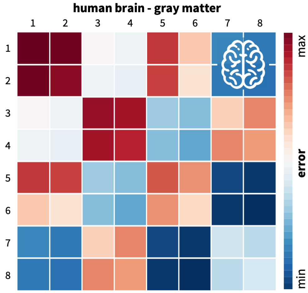
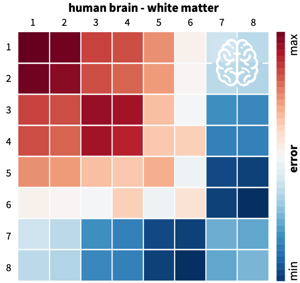
Figure 3: Best-in-class brain models. Discovered one-term models, diagonal, and two-term models, off-diagonal, for isotropic human gray matter. Models are made up of eight functional building blocks: linear, exponential linear, quadratic, and exponential quadratic terms of the first invariant $I_{1}$, rows and columns 1 to 4, and of the second invariant $I_{2}$, rows and columns 5 to 8. The color code indicates the quality of fit to gray matter data [7], ranging from dark blue, best fit, to dark red, worst fit.

Figure 4: Best-in-class brain models. Discovered one-term models, diagonal, and two-term models, off-diagonal, for isotropic human white matter. Models are made up of eight functional building blocks: linear, exponential linear, quadratic, and exponential quadratic terms of the first invariant $I_{1}$, rows and columns 1 to 4, and of the second invariant $I_{2}$, rows and columns 5 to 8. The color code indicates the quality of fit to white matter data [7], ranging from dark blue, best fit, to dark red, worst fit.

Figures 4 and 4 summarize the discovered best-in-class one-term models on the diagonale and the best-in-class two-term models on the off-diagonale. Strikingly, the quality of fit for the one-term models follows exactly the same order for both tissue types: The best-in-class one-term model is the quadratic second-invariant model,

$$\psi=w_{7}\,[\,I_{2}-3\,]^{2}\,,$$

with $w_{7}=19.599$ kPa for gray and $w_{7}=8.671$ kPa for white matter, followed by the exponential quadratic, exponential linear, and linear models, all in the second invariant $I_{2}$, and then by the exponential quadratic, quadratic, exponential linear, and linear models, all in the first invariant $I_{1}$. Notably, the widely used linear first-invariant neo Hooke model [56], $\psi=w_{1}\,[\,I_{1}-3\,]$, with $w_{7}=0.796$ kPa for gray and $w_{7}=0.330$ kPa for white matter, is the worst of all one-term models and Demiray model [9], $\psi=w_{2}\,[\exp(w_{2}^{*}[\,I_{1}-3\,])-1]$, that was designed specifically for soft biological tissues is the second worst. For both tissue types, four models score equally well amongst the best-in-class two-term models: the four combinations of the linear or exponential linear second-invariant term with the quadratic or exponential quadratic second-invariant term. Of those, the simplest model is the linear and quadratic second-invariant model with only two-parameters,

$$\psi=w_{5}\,[\,I_{2}-3\,]+w_{7}\,[\,I_{2}-3\,]^{2}\,,$$

with $w_{5}=0.406$ kPa and $w_{7}=11.178$ kPa for gray and $w_{5}=0.179$ kPa and $w_{7}=4.750$ kPa for white matter. Surprisingly, the popular linear first and second-invariant Mooney Rivlin model [37, 45] performs poorly compared to all other two-term models: For both gray and white matter, its first-invariant parameter is zero, $w_{1}=0.000$ kPa, and only the second-invariant parameter is active, with $w_{5}=0.840$ kPa for gray and $w_{5}=0.354$ kPa for white matter.
What have we discovered? An interesting observation is that the best-in-class plots for gray and white matter in Figures 4 and 4 look remarkably similar, with best fits towards the lower right corner and worst fits towards the upper left. These features are in stark contrast to the best-in-class plot for rubber in Figures 2, which we would not have expected from looking at the data or the fit to a specific model alone. Interestingly, the gold standard approach to first select a model and then fit its parameters to data would have resulted in the two worst performing models, the neo Hooke [56] and Demiray [9] models, which are widely used, but poorly suited for human brain tissue [7]. Instead, our holistic approach discovers a whole new family of second-invariant models that has been overlooked by previous approaches [32]. Strikingly, all second-invariant models consistently outperform the first-invariant models, in both, the best-in-class one-term and two-term categories, both for gray and white matter [36].
Best-in-class artificial meat models. To discover the best model and parameters for artificial meat, we use uniaxial tension, uniaxial compression, and torsion experiments on tofurkey, a plant-based meat substitute of tofu and seitan made from soybean and wheat protein [49].

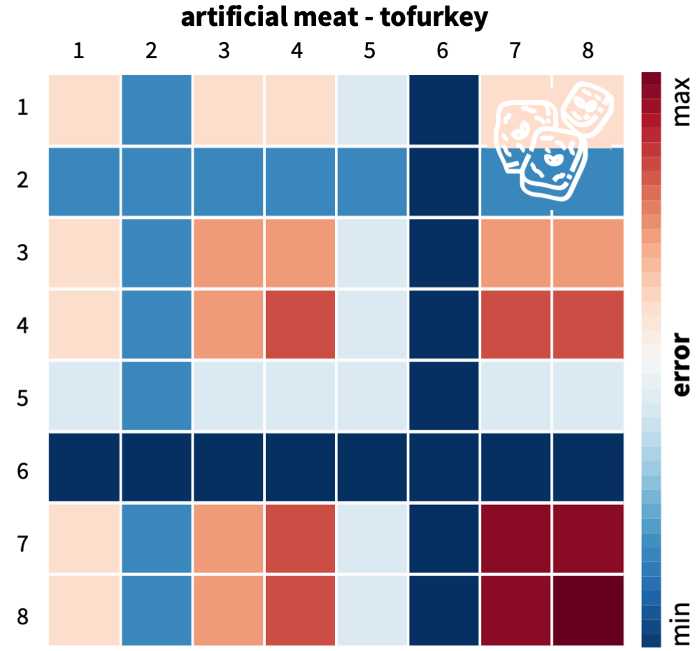
Figure 5: Best-in-class artificial meat models. Discovered one-term models, diagonal, and two-term models, off-diagonal, for isotropic artificial meat tofurkey. Models are made up of eight functional building blocks: linear, exponential linear, quadratic, and exponential quadratic terms of the first invariant $I_{1}$, rows and columns 1 to 4, and of the second invariant $I_{2}$, rows and columns 5 to 8. The color code indicates the quality of fit to white matter data [49], ranging from dark blue, best fit, to dark red, worst fit.

Figure 5 summarizes the discovered best-in-class one-term models on the diagonale and the best-in-class two-term models on the off-diagonale. Interestingly, the best-in-class one-term model is the exponential linear second-invariant model,

$$\psi=w_{6}\,[\exp(w^{*}_{6}\,[\,I_{2}-3\,])-1],$$

with $w_{6}=15.661$ kPa and $w_{6}^{*}=2.020$, closely followed by the exponential linear first-invariant Demiray model [9] with $w_{2}=15.656$ kPa and $w_{2}^{*}=2.021$, the linear second-invariant Blatz Ko model [4] with $w_{5}=32.075$ kPa, and the linear first-invariant neo Hooke model [56] with $w_{1}=32.083$ kPa. Interestingly, the best-in-class two-term models all only contain a single active term, which implies that the additional second term does not improve the overall fit of the model.
What have we discovered? Using our fully automated approach, we have discovered the first ever interpretable model for the plant-based meat substitute tofurkey, a product of soybean and wheat protein. In a naïve approach, we would probably have selected the popular neo Hooke or Mooney Rivlin models to describe this new material. Instead, our automated model discovery reveals that exponential linear models, either in the first or second invariant, provide a better fit than these two models. Unexpectedly, if we were to select a linear model, our study reveals that the second-invariant $[\,I_{2}-3\,]$ Blatz Ko model [4], explains the experimental data better than the first-invariant $[\,I_{1}-3\,]$ neo Hooke model [56]. More broadly, this raises the question why second-invariant models have traditionally been overlooked in constitutive modeling [22].
Best-in-class skin models. To discover the best model and parameters for skin, we use biaxial extension experiments on porcine skin [33, 51].

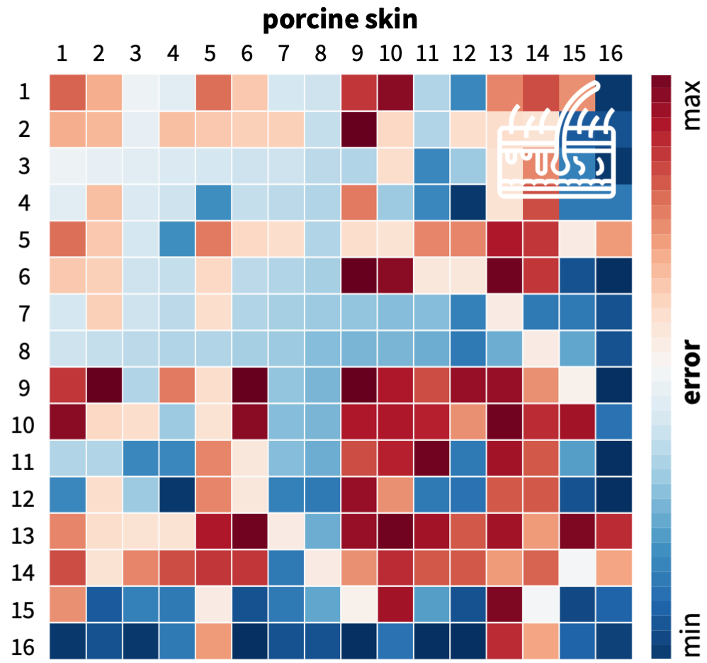
Figure 6: Best-in-class skin models. Discovered one-term models, diagonal, and two-term models, off-diagonal, for transversely isotropic porcine skin. Models are made up of sixteen functional building blocks: linear, exponential linear, quadratic, and exponential quadratic terms of the first invariant $I_{1}$, rows and columns 1 to 4, second invariant $I_{2}$, rows and columns 5 to 8, fourth invariant $I_{4}$, rows and columns 9 to 12, and fifth invariant $I_{5}$, rows and columns 13 to 16. The color code indicates the quality of fit to porcine skin data [51], ranging from dark blue, best fit, to dark red, worst fit.

Figure 6 summarizes the discovered best-in-class one-term models on the diagonale and the best-in-class two-term models on the off-diagonale, where rows and columns 1 to 8 related to the isotropic first and second invariants $I_{1}$ and $I_{2}$ and rows and columns 9 to 16 related to the anisotropic fourth and fifth invariants $I_{4}$ and $I_{5}$. Interestingly, the best-in-class one-term model is the quadratic fifth-invariant model,

$$\psi=w_{15}\,[\,I_{5}-1\,]^{2}$$

with $w_{15}=0.080$ MPa, closely followed by the exponential quadratic fifth-invariant model, with $w_{16}=0.024$ MPa and $w_{16}^{*}=1.934$, and the exponential quadratic fourth-invariant model with $w_{12}=0.185$ MPa and $w_{12}^{*}=1.929$. Only after these three, we find the isotropic one-term models, with the quadratic and exponential quadratic first- and second-invariant models ranking equally well on fourth place. The linear first-invariant neo Hooke model [56] with $w_{1}=0.153$ MPa and the linear second-invariant the Blatz Ko model [4] with $w_{2}=0.141$ MPa share the ninth rank amongst all one-term models. The best in class two-term model combines the exponential quadratic first- and fourth-invariant terms,

$$\psi=w_{4}\,[\exp(w^{*}_{4}\,[\,I_{1}-3\,])^{2}\!-1]+w_{12}\,[\exp(w^{*}_{12}\,[\,I_{4}-3\,])^{2}\!-1],$$

with $w_{4}=0.243$ kPa and $w_{4}^{*}=1.811$ and $w_{12}=0.115$ kPa and $w_{12}^{*}=1.858$. It is followed by a class of models in the last row and column that combine the exponential quadratic fifth-invariant term, $w_{16}\,[\exp(w^{*}_{16}\,[\,I_{5}-3\,])^{2}\!-1]$, with the linear or quadratic first invariant, the exponential linear second invariant, or the linear, quadratic, or exponential quadratic fourth invariant. Notably, neither the classical linear first- and fourth-invariant Lanir model [28] for fibrous connective tissues with $w_{1}=0.078$ MPa and $w_{9}=0.037$ MPa, nor the classical linear first-invariant and exponential quadratic fourth-invariant Holzapfel model [21] for collagenous tissues, with $w_{1}=0.000$ MPa, $w_{12}=0.237$ MPa, and $w_{12}^{*}$=1.783, are amongst the best-in-class two-term models.
What have we discovered? A somewhat unexpected observation is the excellent performance of the quadratic and exponential quadratic fifth-invariant terms in the last two rows and columns. These two terms outperform nearly all other models, both in the one- and two-term categories. The only exception is the best-in-class exponential quadratic first- and fourth-invariant model, a modification of the classical Holzapfel model [21] that replaces the linear isotropic neo Hooke term, $w_{1}\,[\,I_{1}-3\,]$, by a nonlinear isotropic Holzapfel-type term, $w_{4}\,[\exp(w^{*}_{4}\,[\,I_{1}-3\,]^{2})\!-1]$ in the first invariant $I_{1}$. This simple modification of our automated model discovery improves the performance of the classical Holzapfel model and would not have been obvious from looking at the data alone. Microstructurally, our discovery suggests that in skin, not only the collagen fibers, but also the extracellular matrix, display an exponential stiffening with increasing tissue deformation [33].
Best-in-class artery models. To discover the best model and parameters for arteries, we use biaxial extension experiments on the media and adventitia layers of a human artery [38, 44].

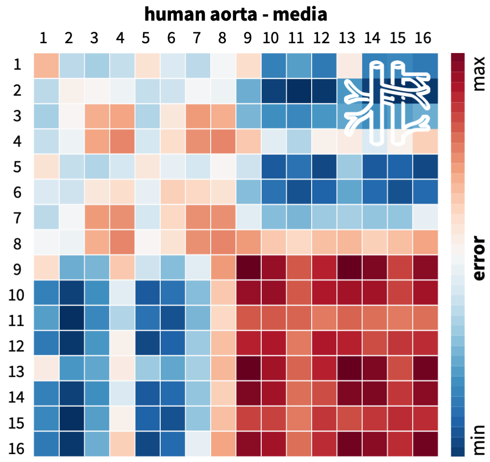
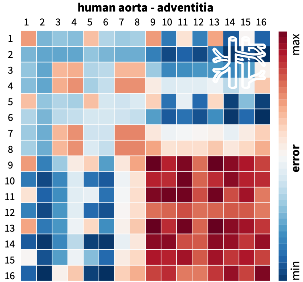
Figure 7: Best-in-class human artery models. Discovered one-term models, diagonal, and two-term models, off-diagonal, for transversely isotropic human arterial media. Models are made up of sixteen functional building blocks: linear, exponential linear, quadratic, and exponential quadratic terms of the first invariant $I_{1}$, rows and columns 1 to 4, second invariant $I_{2}$, rows and columns 5 to 8, fourth invariant $I_{4}$, rows and columns 9 to 12, and fifth invariant $I_{5}$, rows and columns 13 to 16. The color code indicates the quality of fit to human arterial media data [38], ranging from dark blue, best fit, to dark red, worst fit.

Figure 8: Best-in-class human artery models. Discovered one-term models, diagonal, and two-term models, off-diagonal, for transversely isotropic human arterial adventitia. Models are made up of sixteen functional building blocks: linear, exponential linear, quadratic, and exponential quadratic terms of the first invariant $I_{1}$, rows and columns 1 to 4, second invariant $I_{2}$, rows and columns 5 to 8, fourth invariant $I_{4}$, rows and columns 9 to 12, and fifth invariant $I_{5}$, rows and columns 13 to 16. The color code indicates the quality of fit to human arterial adventitia data [38], ranging from dark blue, best fit, to dark red, worst fit.

Figures 8 and 8 summarize the discovered best-in-class one-term models for the media and the adventitia. Strikingly, the four best one-term models are identical for both layers: The best-in-class one-term model is the exponential linear first-invariant Demiray model [9],

$$\psi=w_{2}\,[\exp(w^{*}_{2}\,[\,I_{1}-3\,])\!-1]\,,$$

with $w_{2}=4.929$ kPa and $w_{2}^{*}=3.090$ for the media and $w_{2}=1.866$ kPa and $w_{2}^{*}=2.586$ for the adventitia, followed by the linear first-invariant Blatz Ko model [4] with $w_{5}=22.964$ kPa for the media and $w_{5}=6.336$ kPa for the adventitia, and the exponential linear first-invariant model with $w_{6}=5.462$ kPa and $w_{6}^{*}=2.247$ for the media and $w_{6}=2.713$ kPa and $w_{6}^{*}=1.570$ for the adventitia. The linear first-invariant neo Hooke model [56] only ranks fourth for the media with $w_{1}=29.107$ kPa and fifth for the adventitia with $8.025$ kPa. For both layers, the best-in-class two-term models combine an isotropic exponential linear term, either in $I_{1}$ or $I_{2}$, with an anisotropic quadratic or exponential quadratic term, either in $I_{4}$ or $I_{5}$. An illustrative example is the combination of the exponential linear first-invariant Demiray term [9] with the exponential quadratic fourth-invariant Holzapfel term [21],

$$\psi=w_{2}\,[\exp(w^{*}_{2}\,[\,I_{1}-3\,])\!-1]+w_{12}\,[\exp(w^{*}_{12}\,[\,I_{4}-3\,])^{2}\!-1],$$

with $w_{2}=4.567$ kPa, $w_{2}^{*}=2.934$, $w_{12}=2.399$ kPa, and $w_{12}^{*}=2.146$ for the media and $w_{2}=1.711$ kPa, $w_{2}^{*}=2.469$, $w_{12}=0.249$ kPa, and $w_{12}^{*}=3.969$ for the adventitia. Similar to skin, the classical linear first- and fourth-invariant Lanir model [28] for fibrous connective tissues with $w_{1}=26.757$ kPa and $w_{9}=1.834$ kPa for the media and $w_{1}=7.837$ kPa and $w_{9}=0.127$ kPa for the adventitia fails to explain the experimental data of arteries accurately. While the classical linear first-invariant and exponential quadratic fourth-invariant Holzapfel model [21] for collagenous tissues with $w_{1}=24.403$ kPa, $w_{12}=0.929$ kPa, and $w_{12}^{*}$=4.427 for the media and $w_{1}=6.451$ kPa, $w_{12}=0.150$ kPa, and $w_{12}^{*}$=6.585 for the adventitia performs reasonably well, it does not rank among the best-in-class two-term models.
What have we discovered? Interestingly, the best-in-class plots for the media and adventitia of a human aorta in Figures 8 and 8 look almost identical, with best fits in the upper right and lower left quadrants that combine an isotropic $I_{1}$ or $I_{2}$ term with an anisotropic $I_{4}$ or $I_{5}$ term, and worst fits in the lower right quadrant that combines exclusively anisotropic terms in $I_{4}$ or $I_{5}$. For both aortic layers, these features are much more pronounced than for skin in Figures 6, which we cannot conclude from looking at the data or the fit to a specific model alone. The gold standard model for arterial tissue is the Holzapfel model [21] that combines an isotropic linear first-invariant term and an anisotropic exponential quadratic fourth-invariant term, $\psi=w_{1}\,[\,I_{1}-3\,]+w_{12}\,[\exp(w^{*}_{12}\,[\,I_{4}-3\,])^{2}\!-1]$. Automatic model discovery suggests to replace the linear isotropic neo Hooke term [56], $w_{1}\,[\,I_{1}-3\,]$, with the nonlinear isotropic Demiray term [9], $w_{2}\,[\exp(w^{*}_{2}\,[\,I_{1}-3\,])\!-1]$. The additional second parameter of the Demiray term, the exponential weight factor $w^{*}_{2}$, provides an additional degree of freedom, which results in a better overall fit to the data, as Figures 8 and 8 confirm. Our holistic approach autonomously discovers an exponential isotropic term that has previously been overlooked by transversely isotropic soft tissue models, but promises a much better explanation of the data, with only minor modifications, at no additional computational cost. Interestingly, the nonlinearity in the first invariant has also been acknowledged by the dispersion version of the Holzapfel model [15], $\psi=\frac{1}{2}\,\mu\,[\,I_{1}-3\,]+\frac{1}{2}\,a\,[\,\exp(\,b[\,\kappa\,I_{1}+[1-3\,\kappa]I_{4}-1\,]^{2}\,)-1\,]/{b}$, which introduces a coupling of the first and fourth invariants inside the exponential quadratic term [39]. Microstructurally, our observation suggests that in arteries, not only a single collagen fiber direction, but either fiber dispersion or the entire extracellular matrix, contribute to an isotropic exponential stiffening with increasing tissue deformation [44].

5 Discussion

Distilling knowledge from data lies at the very heart of any scientific discipline [27, 46]. In the context of solid mechanics, this challenge translates into discovering constitutive models that map strains onto stresses [20]. For more than a century, this has been a human-centered process in which a researcher first selects a a mathematical model–or even invents an entirely new one–and then fits its parameters to data [42]. This process is naturally limited to expert specialists, prone to user bias, and vulnerable to human error. Yet, for decades, this has been the gold standard approach; understandably so, because accurate parameter fitting is mathematically challenging and computationally expensive [6]. It is easy to see though that this approach is inherently limited, and even the worlds’s best parameters tell us nothing about the goodness of fit of the model itself [19]. Fortunately, non-convex optimization and statistical learning have massively advanced throughout the past two decades [13, 24, 26], and computational power is no longer a limiting factor. With the recent raise in machine learning and artificial intelligence, it seems natural to re-think the traditional approach, and ask: Whether and how can we discover both model and parameters simultaneously?
When exploring model discovery, importantly, we should not loose sight of our initial objective: Our goal is not to identify just any model that achieves the best fit to the data [19]. In fact, for a finite number of data points, we can always find a model that fits all points exactly. This is precisely what the universal approximation theorem teaches us [23]: A neural network with at least one hidden layer with a sufficient number of nodes and nonlinear activation functions can approximate any continuous function to an arbitrary degree of accuracy. Yet, this is not what we want to do here. Instead, our goal is to discover the best interpretable model with physically meaningful parameters to explain experimental data [6]. We essentially seek sparse models, models that are easy to understand, interpret, and communicate, models that are simple enough to explain the data, but not too simple.
To emphasize simplicity, we start with the simplest of all models that consist of only one term. We select this term from a library of eight terms for isotropic materials, or sixteen terms for transversely isotropic materials [33], using a discrete combinatorics approach [36]. We fit each one-term model by minimizing the loss function, the error between model and data, determine its model parameters, and record the remaining loss. The model with the lowest loss is the best-in-class one-term model, the model with the darkest blue color on the diagonal of the best-in-class plots for rubber, brain, artificial meat, skin, and arteries in Figures 2 to 8. Comparing the best-in-class one-term models already provides a lot more insight than any traditional material modeling approach: Against our intuition, the best-in-class one-term models are different for each family of materials, featuring the first, seventh, sixth, fifteenth, and second terms; yet, they are identical for gray and white matter of the human brain and for the medial and adventitial layers of the human aorta. Strikingly, while the best-in-class linear first-invariant model for rubber, the classical neo Hooke model [56], and the exponential linear first-invariant model for arteries, the Demiray model [9], are well known and widely used, the best-in-class quadratic first-invariant model for the brain, the exponential linear first-invariant model for artificial meat, and the quadratic fifth-invariant model for skin are novel and somewhat unexpected. These result suggest that we more often than not turn to established existing models that are widely used for traditional materials, but are not necessarily the best models for novel families of materials such as artificial meat.
Our observations for the best-in-class one-term models generalize to the two-term models: For both classes of models, it is inexpensive, illustrative, and intuitive to map out the loss function across the 8$\times$8 or 16$\times$16 model discovery space. From a quick side-by-side comparison, we conclude that the best-in-class one- and two-term models are quite different for each family of materials; yet, they are surprisingly similar for both human brain regions [7] and both human artery layers [38]. For all materials, except for artificial meat [49], adding a second term improves the overall fit, as we conclude from the darker blue colors off of the diagonal in Figures 2 to 4 and 6 to 8. In agreement with our intuition, for both skin and arteries, the best-in-class two-term model combines an isotropic first-invariant and an anisotropic fourth-invariant term, both quadratic exponential for skin, and exponential linear and exponential quadratic for arteries. Unexpectedly, neither the best-in-class two-term model for skin nor for arteries features the linear first-invariant neo Hooke term [56] of the original Holzapfel model [21]. Instead, both feature an exponential first-invariant term that suggests that the isotropic extracellular matrix behaves nonlinearly, possibly because of randomly oriented collagen fibers, as suggested by the dispersion version of the Holzapfel model [15]. Notably, for all five materials, we observe a satisfactory reduction of the loss function with only one or two terms. In a recent study of cardiac tissue, with a more complex fully orthotropic microstructure, we have shown that the concept best-in-class modeling generalizes smoothly to three- or more-term models [35]. Taken together, our results suggest that best-in-class modeling provides a quick and intuitive insight into the macroscopic behavior–and possibly even the microstructural architecture–of traditional and new isotropic and transversely isotropic hyperelastic materials.

6 Conclusion

Throughout this manuscript, we have proposed, illustrated, and discussed a novel method to discover interpretable constitutive models from data: best-in-class modeling. In the age of machine learning, a plethora of alternative approaches is currently emerging to derive mathematical models for natural and man-made soft matter systems. While these classical machine learning models provide an excellent fit to the data, most of them are non-generalizable and non-interpretable, they tend to overfit sparse data, and violate physical laws. Here we integrate a century of knowledge in material modeling with recent trends in machine learning and artificial intelligence to discover sparse constitutive models that are generalizable and interpretable by design, while also obeying the fundamental laws of physics. Notably, we do not solve the NP hard discrete combinatorial problem of subset selection by screening all possible combinations of terms. Instead, we start with the best one-term model and iteratively repeat adding terms, to reduce the objective function below a user-defined threshold level. We illustrate the concept of best-in-class modeling for a variety of soft matter systems with eight-term models for rubber, brain, and artificial meat, and sixteen-term models for skin and arteries, which feature 256 and 65,536 possible combinations of terms. Our results suggest that, for all five families of materials, it is sufficient to limit the number of relevant terms to one or two. This implies that we only need to analyze 4 $\times$ 8 one-term and 4 $\times$ 28 two-term isotropic and 3 $\times$ 16 one-term and 3 $\times$ 120 two-term transversely isotropic models, a total of 552 discrete models. Our discovered models reveal several distinct and unexpected features for each family of materials and suggest that best-in-class modeling is an efficient, robust, and easy-to-use strategy to discover the mechanical signatures of traditional and unconventional soft matter systems. Our technology reveals novel insights to characterize, create, and functionalize soft materials and promises to accelerate discovery and innovation of soft matter systems including artificial organs, stretchable electronics, soft robotics, and artificial meat.

References

- [1] Abdusalamov R, Hillgartner M, Itskov M. Automatic generation of interpretable hyperelastic models by symbolic regression. International Journal for Numerical Methods in Engineering 2023;124:2093-2104.
- [2] Alber M, Buganza Tepole A, Cannon W, De S, Dura-Bernal S, Garikipati K, Karniadakis GE, Lytton WW, Perdikaris P, Petzold L, Kuhl E. Integrating machine learning and multiscale modeling: Perspectives, challenges, and opportunities in the biological, biomedical, and behavioral sciences. npj Digital Medicine 2019;2:115.
- [3] As’ad F, Avery P, Farhat C. A mechanics‐informed artificial neural network approach in data‐driven constitutive modeling. International Journal for Numerical Methods in Engineering 2022;123:2738-2759.
- [4] Blatz PJ, Ko WL. Application of finite elastic theory to the deformation of rubbery materials. Transactions of the Society of Rheology 1962;6:223-251.
- [5] Brunton SL, Proctor JP, Kutz JN. Discovering governing equations from data by sparse identification of nonlinear dynamical systems. Proceedings of the National Academy of Sciences 2016;113:3932-3937.
- [6] Brunton SL, Kutz JN. Data-Driven Science and Engineering: Machine Learning, Dynamical Systems, and Control. First Edition, 2019. Cambridge University Press, Massachusetts.
- [7] Budday S, Sommer G, Birkl C, Langkammer C, Jaybaeck J, Kohnert, Bauer M, Paulsen F, Steinmann P, Kuhl E, Holzapfel GA. Mechanical characterization of human brain tissue. Acta Biomaterialia 2017;48:319-340.
- [8] Cauchy AL. Recherches sur l’equilibre et le mouvement intérieur des corps solides ou fluides, élastiques ou non élastiques. Bulletin de la Sociece Philomathique de Paris 1823;9-13.
- [9] Demiray H. A note on the elasticity of soft biological tissues. Journal of Biomechanics 1972;5:309-311.
- [10] Flaschel M, Kumar S, De Lorenzis L. Unsupervised discovery of interpretable hyperelastic constitutive laws. Computer Methods in Applied Mechanics and Engineering 2021;381:113852.
- [11] Flaschel M, Kumar S, De Lorenzis L. Automated discovery of generalized standard material models with EUCLID. Computer Methods in Applied Mechanics and Engineering 2023;405:115867.
- [12] Frank IE, Friedman JH. A statistical view of some chemometrics regression tools. Technometrics 1993;35:109-135.
- [13] Friedman JH. Sparse regression in and classification. International Journal for Forecasting 2012;28:722-738.
- [14] Fuhg JN, Bouklas N. On physics-informed data-driven isotropic and anisotropic constitutive models through probabilistic machine learning and space-filling sampling. Computer Methods in Applied Mechanics and Engineering 2022;394:114915.
- [15] Gasser TC, Ogden RW, Holzapfel GA. Hyperelastic modelling of arterial layers with distributed collagen fibre orientations. Journal of the Royal Society Interface 2006;3:15–35.
- [16] Gent A. A new constitutive relation for rubber. Rubber Chemistry and Technology 1996;69:59–61.
- [17] Hartmann S, Neff P (2003) Polyconvexity of generalized polynomial-type hyperelastic strain energy functions for near-incompressibility. International Journal of Solids and Structures 40: 2767-2791.
- [18] Hastie T, Tibshirani R, Friedman J. The Elements of Statistical Learning. Second Edition; 2009. Springer, New York.
- [19] He H, Zhang Q, Zhang Y, Chen J, Zhang L, Li F. A comparative study of 85 hyperelastic constitutive models for both unfilled fubber and highly filled rubber nanocomposite material. Nano Materials Science 2022;4:64-82.
- [20] Holzapfel GA (2000) Nonlinear Solid Mechanics: A Continuum Approach to Engineering. John Wiley & Sons, Chichester.
- [21] Holzapfel GA, Gasser TC, Ogden RW. A new constitutive framework for arterial wall mechanics and comparative study of material models. Journal of Elasticity 2000;61:1-48.
- [22] Horgan CO, Ogden RW, Saccomandi G. A theory of stress softening of elastomers based on finite chain extensibility Proceedings of the Royal Society London A 2004;460:1737-1754.
- [23] Hornik K, Stinchcombe M, White H. Multilayer feedforward networks are universal approximators. Neural Networks 1989;2:359–366.
- [24] James G, Witten D, Hastie T, Tibshirani R. An Introduction to Statistical Learning. Second Edition; 2013. Springer, New York.
- [25] Klein DK, Fernandez M, Martin RJ, Neff P, Weeger O. Polyconvex anisotropic hyperelasticity with neural networks. Journal of the Mechanics and Physics of Solids 2022;159:105703.
- [26] Korte BH, Vgyen J (2011) Combinatorial Optimization. Springer, Berlin.
- [27] Kramer S, Cerrato M, Dzeroski S, King R. Automated scientific discovery: From equation discovery to autonomous discovery systems. arXiv 2023; doi:10.48550/arXiv.2305.02251.
- [28] Lanir Y. Constitutive equations for fibrous connective tissues. Journal of Biomechanics 1983;16:1-12.
- [29] Linden L, Klein DK, Kalinka KA, Brummund J, Weeger O, Kästner M. Neural networks meet hyperelasticity: A guide to enforcing physics. Journal of the Mechanics and Physics of Solids 2023;179:105363.
- [30] Linka K, Hillgartner M, Abdolazizi KP, Aydin RC, Itskov M, Cyron CJ. Constitutive artificial neural networks: A fast and general approach to predictive data-driven constitutive modeling by deep learning. Journal of Computational Physics 2021;429:110010.
- [31] Linka K, Kuhl E. A new family of Constitutive Artificial Neural Networks towards automated model discovery. Computer Methods in Applied Mechanics and Engineering 2023;403:115731.
- [32] Linka K, St Pierre SR, Kuhl E. Automated model discovery for human brain using Constitutive Artificial Neural Networks. Acta Biomaterialia 2023;160:134-151.
- [33] Linka K, Buganza Tepole A, Holzapfel GA, Kuhl E. Automated model discovery for skin: Discovering the best model, data, and experiment. Computer Methods in Applied Mechanics and Engineering 2023;403:115731.
- [34] Mahnken R. Strain mode-dependent weighting functions in hyperelasticity accounting for verification, validation, and stability of material parameters. Archive of Applied Mechanics 2022;92:713-754.
- [35] Martonova D, Peirlinck M, Linka K, Holzapfel GA, Leyendecker S, Kuhl E. Automated model discovery for human cardiac tissue: Discovering the best model and parameters. itbioRxiv 2024; doi:10.1101/2024.02.27.582427.
- [36] McCulloch JA, St. Pierre SR, Linka K, Kuhl E. On sparse regression, Lp-regularization, and automated model discovery. International Journal for Numerical Methods in Engineering 2024; e7481.
- [37] Mooney M. A theory of large elastic deformations. Journal of Applied Physics 1940;11:582-590.
- [38] Niestrawska JA, Viertler C, Regitnig P, Cohnert TU, Sommer G, Holzapfel GA. Microstructure and mechanics of healthy and aneurysmatic abdominal aortas: experimental analysis and modelling. Journal of the Royal Society Interface 2016;13:20160620.
- [39] Niestrawska JA, Haspinger DC, Holzapfel GA. The influence of fiber dispersion on the mechanical response of aortic tissues in health and disease: a computational study. Computer Methods in Biomechanics and Biomedical Engineering 2018;21:99-112.
- [40] Nikolov DP, Srivastava S, Abeid BA, Scheven UM, Arruda EM, Garikipati K, Estrada JB. Ogden material calibration via magnetic resonance cartography, parameter sensitivity and variational system identification. Philosophical Transactions of the Royal Society A 2022;380:20210324.
- [41] Ogden RW. Large deformation isotropic elasticity – on the correlation of theory and experiment for incompressible rubberlike solids. Proceedings of the Royal Society London Series A 1972;326:565-584.
- [42] Ogden RW, Saccomandi G, Sgura I. Fitting hyperelastic models to experimental data. Computational Mechanics 2004:34:484-502.
- [43] Peirlinck M, Linka K, Hurtado JA, Kuhl E. On automated model discovery and a universal material subroutine for hyperelastic materials. Computer Methods in Applied Mechanics and Engineering. 2024;418:116534.
- [44] Peirlinck M, Linka K, Hurtado JA, Holzapfel GA, Kuhl E. Democratizing biomedical simulation through automated model discovery and a universal material subroutine. bioRxiv 2023; doi:10.1101/2023.12.06.570487.
- [45] Rivlin RS. Large elastic deformations of isotropic materials. IV. Further developments of the general theory. Philosophical Transactions of the Royal Society of London Series A 1948;241:379–397.
- [46] Schmidt M, Lipson H. Distilling free-form natural laws from experimental data. Science 2009;324:81-85.
- [47] Spencer AJM (1971) Theory of Invariants. In: Eringen AC, Ed., Continuum Physics Vol. 1: 239-353, Academic Press, New York.
- [48] Steinmann P, Hossain M, Possart G. Hyperelastic models for rubber-like materials: consistent tangent operators and suitability for Treloar’s data. Archive of Applied Mechanics 2012;82:1183-1217.
- [49] St Pierre SR, Rajasekharan D, Darwin EC, Linka K, Levenston ME, Kuhl E. Discovering the mechanics of artificial and real meat. Computer Methods in Applied Mechanics and Engineering 2023;415:116236.
- [50] St Pierre SR, Linka K, Kuhl E. Principal-stretch-based constitutive neural networks autonomously discover a subclass of Ogden models for human brain tissue. Brain Multiphysics 2023;4:100066.
- [51] Tac V, Sahli Costabal F, Buganza Tepole A. Data-driven tissue mechanics with polyconvex neural ordinary differential equations. Computer Methods in Applied Mechanics and Engineering 2022;398:115248.
- [52] Tac V, Sree FC, Rausch MK, Buganza Tepole A. Data-driven modeling of the mechanical behavior of anisotropic soft biological tissue. Engineering with Computers 2022;73:49-65.
- [53] Tac V, Linka K, Sahli Costabal F, Kuhl E, Buganza Tepole A. Benchmarking physics-informed frameworks for data-driven hyperelasticity. Computational Mechanics 2024;73:49-65.
- [54] Tibshirani R. Regression shrinkage and selection via the lasso. Journal of the Royal Statistical Society B 1996;58:267-288.
- [55] Treloar LRG. Stress-strain data for vulcanised rubber under various types of deformation. Transactions of the Faraday Society 1944;40:59-70.
- [56] Treloar LRG. Stresses and birefringence in rubber subjected to general homogeneous strain. Proceedings of the Physical Society 1948;60:135-144.
- [57] Truesdell C, Noll W. non linear field theories of mechanics. In: Flügge S, Ed., Encyclopedia of Physics, Vol. III/3; 1965. Spinger, Berlin.
- [58] Valanis K, Landel RF. The strain-energy function of a hyperelastic material in terms of the extension ratios. Journal of Applied Physics 1967;38:2997–3002.
- [59] Wang Z, Estrada JB, Arruda EM, Garikipati K. Inference of deformation mechanisms and constitutive response of soft material surrogates of biological tissue by full-field characterization and data-driven variational system identification. Journal of the Mechanics and Physics of Solids 2021;153:104474.
- [60] Zhang L, Schaeffer H. On the convergence of the SINDy algorithm. Multiscale Modeling and Simulation 2019;17:948-972.