Dual Ensemble Kalman Filter for Stochastic Optimal Control

Abstract

In this paper, stochastic optimal control problems in continuous time and space are considered. In recent years, such problems have received renewed attention from the lens of reinforcement learning (RL) which is also one of our motivation. The main contribution is a simulation-based algorithm – dual ensemble Kalman filter (EnKF) – to numerically approximate the solution of these problems. The paper extends our previous work where the dual EnKF was applied in deterministic settings of the problem. The theoretical results and algorithms are illustrated with numerical experiments.

I Introduction

Many types of reinforcement learning (RL) algorithms may be viewed as “simulation-based” where a model of a control system is simulated to evaluate and iteratively improve a policy. In continuous-type continuous-space settings of this paper, the optimal policy may be obtained from solving the Hamilton-Jacobi-Bellman (HJB) equation for the value function (in linear Gaussian settings, the equation reduces to a differential Riccati equation (DRE)). A simulation-based algorithm is useful for approximating the solution of the HJB or the DRE for the cases where the state-space is too large or the model parameters are not explicitly available (even though a simulator for the same is).

In this paper, we consider optimal control problems where the the control system is an Itô stochastic differential equation (SDE) as follows:

$$\mathrm{d}X_{t} =(a(X_{t})+b(X_{t})U_{t})\mathrm{d}t+\sigma(X_{t})\mathrm{d}W_{t},$$ (1a)

$$X_{0} =x$$ (1b)

where $X:=\{X_{t}:0\leq t\leq T\}$ is the $\mathbb{R}^{d}$-valued state process, $U:=\{U_{t}:0\leq t\leq T\}$ is the $\mathbb{R}^{m}$-valued control input, $W:=\{W_{t}:t\geq 0\leq t\leq T\}$ is a standard Brownian motion (B.M.), and $a(\cdot),b(\cdot),\sigma(\cdot)$ are twice continuously differentiable functions of their arguments. The model is said to be deterministic if $\sigma(x)=0$ for all $x\in\mathbb{R}^{d}$. The model is said to be linear Gaussian if $a(x)=Ax$, $b(x)=B$, and $\sigma(x)=\sigma$.

Our objective in this paper is to design a simulation-based algorithm to approximate (or learn) the optimal control law. Two types of control objectives are considered for this purpose: (i) stochastic optimal control (SOC); and (ii) risk sensitive control (RSC), both over a finite-time horizon $[0,T]$. The infinite-horizon case is obtained by letting $T\to\infty$.

The help explain the main idea of this paper, consider the SOC problem. Let $v_{t}(\cdot)$ denote the optimal value function for this problem (for the linear Gaussian model with quadratic cost (LQG), the value function $v_{t}(x)=x^{\intercal}P_{t}x+g_{t}$ is quadratic). Instead of computing $v_{t}(x)$ by solving the HJB (or the DRE) equation, our perspective is to view $\exp(-v_{t}(x))$ as an un-normalized form of a probability density, denoted as $p_{t}(x)$. That is,

$$p_{t}(x)=\frac{\exp(-v_{t}(x))}{\int_{\mathbb{R}^{d}}\exp(-v_{t}(z))\mathrm{d}z},\quad x\in\mathbb{R}^{d},\;0\leq t\leq T$$

(For LQG, assuming $P_{t}$ is invertible, $p_{t}={\cal N}(0,P_{t}^{-1})$ is a Gaussian density).

I-A Contribution of this paper

Our aim is to approximate the density $p_{t}(\cdot)$ as an ensemble $\{Y_{t}^{i}\in\mathbb{R}^{d}:0\leq t\leq T,1\leq i\leq N\}$ such that

$$Y_{t}^{i}\stackrel{{\scriptstyle\text{i.i.d.}}}{{\sim}}p_{t}(\cdot),\quad i=1,2,\ldots,N,\quad 0\leq t\leq T$$ (2)

(For LQG, $Y_{t}^{i}\stackrel{{\scriptstyle\text{i.i.d.}}}{{\sim}}{\cal N}(0,P_{t}^{-1})$ for $0\leq t\leq T$).

The proposed simulation-based algorithm is a backward-in-time controlled interacting particle system:

$$\mathrm{d}Y^{i}_{t} =\underbrace{a(Y_{t}^{i})\mathrm{d}t+b\mathrm{d}\overset{\shortleftarrow}{\eta}_{t}^{i}+\sigma(Y_{t}^{i})\mathrm{d}\overset{\shortleftarrow}{W}_{t}^{i}}_{i-\text{th copy of model}~{}\eqref{eq:dyn}}+\underbrace{{\cal A}_{t}(Y_{t}^{i};p_{t}^{(N)})\mathrm{d}t}_{\text{mean field term}}$$ (3a)

$$Y_{T}^{i} \stackrel{{\scriptstyle\text{i.i.d.}}}{{\sim}}\frac{\exp(-\mathcal{G}(\cdot))}{\int_{\mathbb{R}^{d}}\exp(-\mathcal{G}(z))\mathrm{d}z},\quad i=1,2,\ldots,N,$$ (3b)

where $\mathcal{G}$ is the terminal condition for the value function (for LQG it is a quadratic function of the state), and $p_{t}^{(N)}$ is the empirical distribution of the ensemble. The design problem is to design $\eta:=\{(\eta_{t}^{i},:0\leq t\leq T\}$ and ${\cal A}:=\{{\cal A}_{t}:0\leq t\leq T\}$ such that (2) holds in the mean-field limit ($N=\infty$).

The first such algorithm appears in our prior work [1] where explicit forms of ${\eta}$ and ${\cal A}$ are described for the deterministic setting of the problem. The resulting algorithm is referred to as the dual ensemble Kalman filter (EnKF). The contribution of this paper is to extend the dual EnKF to stochastic setting for the SOC and RSC problems. The specific types of cost structures are introduced in Sec. II.

I-B Relationship to literature

The idea of transforming an optimal control problem into a sampling problem is not new. For the SOC problem, the idea has its roots in the log transform which appears in [2] and is related to the minimum energy duality which is even older [3, 4]. These types of transformations are routinely re-discovered and have been applied for solving sampling/inference problems as optimal control problems and vice-versa (see [5, 6, 7, 8, 9, 10] and [11] for a review). In the control community, the moving horizon estimator is an example of the minimum energy duality [12, Ch. 4].

What is perhaps new in [1] are two aspects of (3):

1. Design of ${\eta}_{t}^{i}$ as a B.M. This may be regarded as the exploration signal in RL.

2. Design of ${\cal A}_{t}(\cdot;\cdot)$. This is the idea of designing interactions between simulations to approximate the solution of the HJB equation.

In numerical performance and theoretical guarantees, these algorithms can be order of magnitude better than the competing approaches (detailed comparisons can be found in [1, Table 1]). There are some recent papers from other groups [13, 14] which also use interacting particle systems to solve stochastic optimal control problems, a detailed comparison to which is presented in the main body of the paper.

It is noted that while the use of EnKF and controlled interacting particle systems appears to be new for optimal control and RL, EnKF is a standard simulation-based algorithm in the filtering (data assimilation) applications [15].

I-C Organisation of paper

The outline of the remainder of this paper is as follows. The mathematical formulations for the SOC and RSC problems appear in Sec. II. The simulation-based algorithm to approximate its solution appears in Sec. III. Each of these sections include a discussion of historical and recent literature on these topics. The algorithms are numerically illustrated in Sec. IV.

II Problem Formulation

Notation: Given a symmetric positive semi-definite matrix $Q$, we let $|z|_{Q}\coloneqq z^{\intercal}Qz$. The normal distribution is represented as $\mathcal{N}(\cdot,\cdot)$ where the first argument is the mean and second is the covariance. We let $\text{Cov}(\cdot)$ represent covariance.

II-A Deterministic Optimal Control (DOC)

The simplest formulation is the deterministic case obtained when $\sigma=0$. In this case, the SDE (1) reduces to an ordinary differential equation and $X$ and $U$ are both deterministic processes. The deterministic optimal control objective is as follows:

$$J_{T}^{\text{\tiny DOC}}(U):=\int_{0}^{T}{\mathchoice{\genfrac{}{}{}{1}{1}{2}}{\genfrac{}{}{}{2}{1}{2}}{\genfrac{}{}{}{3}{1}{2}}{\genfrac{}{}{}{4}{1}{2}}}\left(|c(X_{t})|^{2}+|U_{t}|^{2}_{R}\right)\mathrm{d}t+\,\mathcal{G}(X_{T})$$

where $c,\mathcal{G}$ are twice continuously differentiably real valued function, with $\mathcal{G}$ taking only non-negative value and $R$ is a symmetric strictly positive definite matrix.

In a prior work [1], a simulation-based algorithm for approximation of the optimal control law is described. The algorithm is referred to as the dual ensemble Kalman filter or dual EnKF for short. The goal of the present paper is to generalize and extend the dual EnKF to the stochastic optimal control problem for the system (1) when $\sigma\neq 0$. For this purpose, the following types of cost structures are considered.

II-B Stochastic Optimal Control (SOC)

The stochastic optimal control objective is as follows:

$$J_{T}^{\text{\tiny SOC}}(U):={\sf E}\left(J_{T}^{\text{\tiny DOC}}(U)\right)$$

where randomness enters due to the Brownian motion in (1), and as noted earlier, we require the control to be adapted to the filtration generated by the Brownian motion.

II-C Risk Sensitive Control (RSC)

For risk sensitive control, the following objective is of interest [16, Equation (1)]:

$$J_{T}^{\text{\tiny RSC}}(U)=\theta^{-1}\log{\sf E}\left(\exp{(\theta J_{T}^{\text{\tiny DOC}}(U))}\right)$$

where $\theta\in\mathbb{R}\setminus\{0\}$ is referred to as the risk sensitive parameter. The case $\theta>0$ is known as risk averse and $\theta<0$ as risk seeking. A rigorous treatment of this problem, along with its motivations, appear in [16], [17, Section 8]. We note that the cost is always non-negative for every $\theta\neq 0$ because $\exp{(\theta J_{T}^{\text{\tiny DOC}}(U))}>1$ if $\theta>0$ and $\exp{(\theta J_{T}^{\text{\tiny DOC}}(U))}<1$ when $\theta<0$ for all $U$.

II-D Linear Quadratic (LQ) Control

Suppose the system (1) has linear time invariant dynamics (LTI), that is, $a(z)=Az$, $b(z)u=Bu$ and $\sigma(z)=\sigma$, and the cost has a quadratic structure, that is, $|c(z)|^{2}=|Cz|^{2}$ and $\mathcal{G}(z)=|z|_{G}^{2}$ for matrices $A,B,\sigma,C,G$ where $G^{\intercal}=G\succ 0$.

Assumption 1

$(A,B)$ is controllable, $(A,C)$ is observable, and $BR^{-1}B^{\intercal}-\theta\sigma\sigma^{\intercal}\succ 0$.

The last assumption is needed to ensure positive definiteness of the solution to the Riccati equation, which is introduced in subsequent sections [18, Equation (90)]. In this case SOC is called linear quadratic Gaussian (LQG) and RSC is called linear quadratic exponential Gaussian (LEQG).

II-E Literature survey

SOC: SOC is a standard and well studied problem in stochastic control theory [19, 20, 21]. Two approaches to solve it are using the stochastic maximum principle, and stochastic HJB equation [20].

RSC: The RSC has a long history going back to early works like [18] and [22]. A more recent introduction to LEQG can be found in [16], [17],[23], and for some recent surveys on the topic, see [24], [25], [26]. A stochastic maximum principle for LEQG was established in [27], and [28] solved the problem using fundamental ideas like completion of squares and Girsanov theorem. The connection of LEQG to games is also a well studied area, see for example, [18], [23], in which the connection to linear quadratic zero sum differential games is demonstrated, and [29] for how non-linear exponential cost problem relate to differential games.

III Proposed methodology

	$\mathcal{H}(v)$
SOC	${\mathchoice{\genfrac{}{}{}{1}{1}{2}}{\genfrac{}{}{}{2}{1}{2}}{\genfrac{}{}{}{3}{1}{2}}{\genfrac{}{}{}{4}{1}{2}}}|c|^{2}+(\nabla v)^{\intercal}a-{\mathchoice{\genfrac{}{}{}{1}{1}{2}}{\genfrac{}{}{}{2}{1}{2}}{\genfrac{}{}{}{3}{1}{2}}{\genfrac{}{}{}{4}{1}{2}}}(\nabla v)^{\intercal}D\nabla v+{\mathchoice{\genfrac{}{}{}{1}{1}{2}}{\genfrac{}{}{}{2}{1}{2}}{\genfrac{}{}{}{3}{1}{2}}{\genfrac{}{}{}{4}{1}{2}}}\mathrm{tr}(\Sigma\nabla^{2}v)$
RSC	${\mathchoice{\genfrac{}{}{}{1}{1}{2}}{\genfrac{}{}{}{2}{1}{2}}{\genfrac{}{}{}{3}{1}{2}}{\genfrac{}{}{}{4}{1}{2}}}|c|^{2}+(\nabla v)^{\intercal}a-\frac{1}{2}(\nabla v)^{\intercal}(D-\theta\Sigma)\nabla v+\frac{1}{2}\mathrm{tr}(\Sigma\nabla^{2}v)$

TABLE I: The right-hand-side of the HJB equation (4) for the SOC and RSC problems. The notations $D\coloneqq bR^{-1}b^{\intercal}$ and $\Sigma\coloneqq\sigma\sigma^{\intercal}$.

The proposed methodology is presented in three subsections. In Sec. III-A, we relate the value function for the optimal control problems to a probability density function. In Sec. III-B, we relate the probability density function to a suitably designed stochastic process that can be simulated as an interacting particle system. Finally, in Sec. III-C, we present the specialization to the LQ setting, followed by a Gaussian approximation procedure that can be applied to nonlinear setup.

III-A Transforming value function to probability density

Consider the SOC and RSC problems. Value function $\{v_{t}(x):0\leq t\leq T,x\in\mathbb{R}^{d}\}$ is defined as the optimal cost-to-go over the horizon $[t,T]$ when the state $X_{t}=x$. According to the dynamic programming principle, the value function satisfies the Hamilton Jacobi Bellman (HJB) partial differential equation (PDE)

$$-\frac{\partial v}{\partial t}=\mathcal{H}(v),\quad v_{T}=\mathcal{G}$$ (4)

where $\mathcal{H}$ is given in Table I [16, Equation (3)],[20, Equation (11.2.5)]. The optimal control is obtained as a function of $v$ as

$$U_{t}^{*}=-R^{-1}b(X_{t})^{\intercal}v_{t}(X_{t}).$$ (5)

In this paper, our strategy is to introduce a bijection $\psi:\mathbb{R}\to\mathbb{R}$ so that

$$p_{t}(x):=\frac{\psi(v_{t}(x))}{\int\psi(v_{t}(x))\mathrm{d}x},\quad 0\leq t\leq T,\;x\in\mathbb{R}^{d}$$ (6)

has the meaning of a probability density function. The bijection $\psi$ is selected according to

$$\psi(z)\coloneqq\begin{cases}\exp(-z);&\text{SOC}\\ \exp(-|\theta|z);&\text{RSC}\end{cases}$$ (7)

Our choice of $\psi$ is inspired from the log transform which is routinely used in risk sensitive control [17]. Since the value function is always positive, $\psi$ has been appropriately adjusted so that the quantity inside the exponential is negative. We also note that our method is only intended for situations when $\psi(v_{t}(\cdot))\in L^{1}(\mathbb{R})$ for all $0\leq t\leq T$.

Cost	${\mathcal{D}}(\Lambda)$
LQG	$A^{\intercal}\Lambda+\Lambda A+C^{\intercal}C-\Lambda BR^{-1}B^{\intercal}\Lambda$
LEQG	$A^{\intercal}\Lambda+\Lambda A+C^{\intercal}C-\Lambda(BR^{-1}B^{\intercal}-\theta\sigma\sigma^{\intercal})\Lambda$

TABLE II: Expression for DRE in (11)

III-B Mean-field process

The goal is to design a (mean-field) stochastic process that has the same density function as $\{p_{t}:0\leq t\leq T\}$.

Cost	${\mathcal{D}^{\dagger}}(\Lambda)$
LQG	$A\Lambda+\Lambda A^{\intercal}-BR^{-1}B^{\intercal}+\Lambda C^{\intercal}C\Lambda$
LEQG	$A\Lambda+\Lambda A^{\intercal}-\frac{1}{|\theta|}(BR^{-1}B^{\intercal}-\theta\sigma\sigma^{\intercal})+|\theta|\Lambda C^{\intercal}C\Lambda$

TABLE III: Expression for the Dual DRE in (12)

Define a stochastic process ${Y}=\{{Y}_{t}\in\mathbb{R}^{d}:0\leq t\leq T\}$ as a solution of the following backward (in time) SDE:

$$\mathrm{d}{Y}_{t} =a({Y}_{t})\mathrm{d}t+b({Y}_{t})\mathrm{d}\overset{\shortleftarrow}{{\eta}}_{t}+\sigma({Y}_{t})\mathrm{d}\overset{\shortleftarrow}{W}_{t}$$

$$\qquad+(\mathcal{I}_{t}({Y}_{t};\bar{p}_{t})+\mathcal{C}_{t}({Y}_{t};\bar{p}_{t}))\mathrm{d}t$$ (8a)

$${Y}_{T} \sim\frac{\psi(\mathcal{G}(\cdot))}{\int\psi(\mathcal{G}(z))\mathrm{d}z}$$ (8b)

where ${{\eta}}=\{{{\eta}}_{t}\in\mathbb{R}^{m}:0\leq t\leq T\}$ is a B.M. with a suitably chosen covariance matrix, $\mathcal{I}_{t}(\cdot;\cdot),\mathcal{C}_{t}(\cdot;\cdot)$ is a suitably chosen vector field, and $\bar{p}_{t}$ is the density of ${Y}$. Here we have written the mean field term $\mathcal{A}$ introduced earlier as a sum of $\mathcal{I}+\mathcal{C}$, and the reason for which will be made clear later in this exposition. The meaning of the backward arrow on $\mathrm{d}\overset{\shortleftarrow}{{\eta}},\mathrm{d}\overset{\shortleftarrow}{W}$ in (8) is that the SDE is simulated backward in time starting from the terminal condition specified at time $t=T$. The reader is referred to [30, Sec. 4.2] for the definition of the backward Itô-integral. The mean-field process is useful because of the following proposition.

Proposition 1

Consider the mean-field process (8). Suppose $\text{Cov}(\eta)$ is Selected according to Table V, $\mathcal{I}$ and $\mathcal{C}$ satisfy the PDEs

$$-\nabla\cdot(\bar{p}_{t}(\cdot)\mathcal{I}_{t}(\cdot;\bar{p}_{t})) =\bar{p}_{t}(h_{t}(\cdot)-\hat{h}_{t}),$$ (9a)

$$-\nabla\cdot(\bar{p}_{t}(\cdot)\mathcal{C}_{t}(\cdot;\bar{p}_{t})) =\mathcal{V}_{t}(\cdot),$$ (9b)

where $\mathcal{V}_{t}(\cdot)$, $h$ also appear in Table V, and $\hat{h}_{t}\coloneqq\int\bar{p}_{t}(z)h_{t}(z)\mathrm{d}z$. Then,

$$\bar{p}_{t}=p_{t},\quad\forall t\in[0,T],$$ (10)

where $\bar{p}_{t}$ is the probability density function of ${Y}_{t}$ and $p_{t}$ is defined in (6) in terms of the value function. The optimal control is expressed as a function of $\bar{p}_{t}$ according to

$$U_{t}^{*}=\begin{cases}R^{-1}b(X_{t})^{\intercal}\nabla\log\bar{p}_{t}(X_{t});&\text{SOC}\\ (|\theta|R)^{-1}b(X_{t})^{\intercal}\nabla\log\bar{p}_{t}(X_{t});&\text{RSC}\\ \end{cases}$$

Proof:

See Appendix A. ∎

The significance of Prop. 1 is that the optimal control policy $\phi_{t}(\cdot)$ can now be obtained in terms of the statistics of the random variable ${Y}_{t}$. The PDEs written may not always be analytically tractable, in which case, one has to rely on numerical approximation techniques. We call $\mathcal{I}$ as the interaction term, and $\mathcal{C}$ as the correction term, since the latter accounts for non-constant system model. In other words, if $b,\sigma$ are constants, then $\mathcal{C}$ becomes 0 for RSC with $\theta<0$, and otherwise $\mathcal{V}$ simplifies to $\mathrm{tr}(\nabla^{2}\bar{p}_{t})$ for RSC with $\theta>0$ and ${\mathchoice{\genfrac{}{}{}{1}{1}{2}}{\genfrac{}{}{}{2}{1}{2}}{\genfrac{}{}{}{3}{1}{2}}{\genfrac{}{}{}{4}{1}{2}}}\mathrm{tr}(\nabla^{2}\bar{p}_{t})$ for SOC.

	$\mathcal{I}_{t}^{\text{LQ}}(z;n_{t},S_{t})$	$\mathcal{C}_{t}^{\text{LQ}}(z;n_{t},S_{t})$
LQG	${\mathchoice{\genfrac{}{}{}{1}{1}{2}}{\genfrac{}{}{}{2}{1}{2}}{\genfrac{}{}{}{3}{1}{2}}{\genfrac{}{}{}{4}{1}{2}}}S_{t}C^{\intercal}C(z+n_{t})$	${\mathchoice{\genfrac{}{}{}{1}{1}{2}}{\genfrac{}{}{}{2}{1}{2}}{\genfrac{}{}{}{3}{1}{2}}{\genfrac{}{}{}{4}{1}{2}}}\Sigma S_{t}^{-1}(z-n_{t})$
LEQG	$\frac{|\theta|}{2}S_{t}C^{\intercal}C(z+n_{t})$	$\Sigma S_{t}^{-1}(z-n_{t})$
$\theta>0$
LEQG		$0$
$\theta<0$

TABLE IV: Vector fields for LQ case in (13).

Cost	$\mathcal{V}(\cdot)$	$h_{t}(\cdot)$	$\text{Cov}(\eta)$
LQG	${\mathchoice{\genfrac{}{}{}{1}{1}{2}}{\genfrac{}{}{}{2}{1}{2}}{\genfrac{}{}{}{3}{1}{2}}{\genfrac{}{}{}{4}{1}{2}}}\nabla^{2}\cdot(\Sigma\bar{p}_{t})$	${\mathchoice{\genfrac{}{}{}{1}{1}{2}}{\genfrac{}{}{}{2}{1}{2}}{\genfrac{}{}{}{3}{1}{2}}{\genfrac{}{}{}{4}{1}{2}}}|c|^{2}+\nabla\cdot a+{\mathchoice{\genfrac{}{}{}{1}{1}{2}}{\genfrac{}{}{}{2}{1}{2}}{\genfrac{}{}{}{3}{1}{2}}{\genfrac{}{}{}{4}{1}{2}}}\mathrm{tr}((D-\Sigma)\nabla^{2}\log(\bar{p}_{t}))$	$R^{-1}$
LEQG	$\nabla\cdot(\bar{p}_{t}\nabla\cdot(\Sigma-\frac{1}{\theta}D))$	$-\frac{\theta}{2}|c|^{2}+\nabla\cdot a+{\mathchoice{\genfrac{}{}{}{1}{1}{2}}{\genfrac{}{}{}{2}{1}{2}}{\genfrac{}{}{}{3}{1}{2}}{\genfrac{}{}{}{4}{1}{2}}}\nabla^{2}\cdot(\frac{1}{\theta}D-\Sigma)-\frac{1}{2\theta}\mathrm{tr}(D\nabla^{2}\log\bar{p}_{t})$	$(\sqrt{|\theta|}R)^{-1}$
$\theta<0$
LEQG	$\nabla^{2}\cdot(\bar{p}_{t}\Sigma)+\nabla\cdot(\bar{p}_{t}\nabla\cdot(\frac{1}{\theta}D-\Sigma))$	$\frac{\theta}{2}|c|^{2}+\nabla\cdot a-\nabla^{2}\cdot(\frac{1}{\theta}D-\Sigma)+{\mathchoice{\genfrac{}{}{}{1}{1}{2}}{\genfrac{}{}{}{2}{1}{2}}{\genfrac{}{}{}{3}{1}{2}}{\genfrac{}{}{}{4}{1}{2}}}\mathrm{tr}((\frac{1}{\theta}D-2\Sigma)\nabla^{2}\log\bar{p}_{t})$	$(\sqrt{|\theta|}R)^{-1}$
$\theta>0$

TABLE V: Details for the Poisson equation (9) in Proposition 1.

III-C LQ setting

In this scenario, the value function is obtained as

$$v_{t}(x)={\mathchoice{\genfrac{}{}{}{1}{1}{2}}{\genfrac{}{}{}{2}{1}{2}}{\genfrac{}{}{}{3}{1}{2}}{\genfrac{}{}{}{4}{1}{2}}}x^{\intercal}P_{t}x+g_{t}$$

where $\{P_{t}:0\leq t\leq T\}$ is a matrix valued process which is the solution of the backward (in time) differential Riccati equation (DRE)

$$-\frac{\mathrm{d}}{\mathrm{d}t}P_{t}=\mathcal{D}(P_{t}),\quad P_{T}=G$$ (11)

where the expressions for the $\mathcal{D}(\cdot)$ are in Table II, and

$$-\dot{g}_{t}=\mathrm{tr}(\sigma\sigma^{\intercal}P_{t}),\quad g_{T}=0.$$

Under the Assumption 1, $P_{t}\succ 0$ for $0\leq t\leq T$ whenever $G\succ 0$ [31, Sec. 24], [18, Equation (90)]. Then density $p_{t}$ obtained from the value function then always takes the form $\mathcal{N}(0,S_{t})$, where

$$S_{t}:=\begin{cases}P_{t}^{-1};\quad&\text{LQG}\\ (|\theta|P_{t})^{-1};\quad&\text{LEQG}\end{cases},\quad 0\leq t\leq T.$$

It is readily verified that $\{S_{t}:0\leq t\leq T\}$ also solves a DRE

$$-\frac{\mathrm{d}}{\mathrm{d}t}S_{t}=\mathcal{D}^{\dagger}(S_{t}),$$ (12)

which represents the dual of (11), and the expressions for $\mathcal{D}^{\dagger}$ appear in Table III. The expressions for $\mathcal{I},\mathcal{C},\eta$ in this scenario are denoted by a superscript ${}^{\text{LQ}}$ and appear in Table IV. The derivations of these expressions appear in Appendix A.

The mean-field process is empirically approximated by simulating a system of controlled interacting particles according to

$$\mathrm{d}{Y}^{i}_{t}=\underbrace{A{Y}^{i}_{t}\mathrm{d}t+B\mathrm{d}\overset{\shortleftarrow}{\eta}^{i}_{t}+\sigma\mathrm{d}\overset{\shortleftarrow}{W}^{i}_{t}}_{\text{i-th copy of model}~{}\eqref{eq:dyn}}$$

$$+\underbrace{\mathcal{I}_{t}^{\text{LQ}}({Y}^{i}_{t};n_{t}^{(N)},S_{t}^{(N)})+\mathcal{C}_{t}^{\text{LQ}}({Y}^{i}_{t};n_{t}^{(N)},S_{t}^{(N)})\mathrm{d}t}_{\text{data assimilation process}}$$ (13a)

$${Y}^{i}_{T}\stackrel{{\scriptstyle\text{i.i.d}}}{{\sim}}\mathcal{N}(0,S_{T}),\quad 1\leq i\leq N,$$ (13b)

${\eta}^{i}$ and $W^{i}$ are an i.i.d copy of ${{\eta}}$ and $W$ respectively, $n^{(N)}_{t}:=N^{-1}\sum_{i=1}^{N}{Y}^{i}_{t}$, and

$$S^{(N)}_{t}:=\frac{1}{N-1}\sum_{i=1}^{N}({Y}^{i}_{t}-n^{(N)}_{t})({Y}^{i}_{t}-n^{(N)}_{t})^{\top}$$ (14)

The data assimilation process serves to couple the particles. Without it, the particles are independent of each other. The finite-$N$ system (13) is referred to as the dual EnKF.

Optimal control: Set ${X}^{i}_{t}:=(S^{(N)}_{t})^{-1}({Y}^{i}_{t}-n^{(N)}_{t})$. Define

$$\tilde{K}^{(N)}_{t}\coloneqq\begin{cases}\dfrac{1}{N-1}\sum_{i=1}^{N}{X}^{i}_{t}({X}^{i}_{t})^{\intercal},&\,\,\text{LQG}\\ \vskip 5.0pt\cr\dfrac{1}{(N-1)|\theta|}\sum_{i=1}^{N}{X}^{i}_{t}({X}^{i}_{t})^{\intercal},&\,\,\text{LEQG}\\ \end{cases}$$ (15)

We consider two cases:

1. If the matrix $B$ is explicitly known then

   $$K_{t}^{(N)}=-R^{-1}B^{\intercal}\tilde{K}^{(N)}_{t}$$ (16)

   from which the optimal control policy is approximated as $\phi_{t}^{(N)}(x)=K_{t}^{(N)}x.$

2. If $B$ is unknown, define the Hamiltonian

   $$H^{(N)}(x,\alpha,t) :=\underbrace{{\mathchoice{\genfrac{}{}{}{1}{1}{2}}{\genfrac{}{}{}{2}{1}{2}}{\genfrac{}{}{}{3}{1}{2}}{\genfrac{}{}{}{4}{1}{2}}}|Cx|^{2}\quad+{\mathchoice{\genfrac{}{}{}{1}{1}{2}}{\genfrac{}{}{}{2}{1}{2}}{\genfrac{}{}{}{3}{1}{2}}{\genfrac{}{}{}{4}{1}{2}}}\alpha^{\intercal}R\alpha}_{\text{cost function}}$$

   $$\quad+x^{\intercal}\tilde{K}^{(N)}_{t}\underbrace{(Ax+B\alpha)}_{\text{model}~{}\eqref{eq:dyn}}$$

   from which the optimal control policy is approximated as

   $$\phi_{t}^{(N)}(x)=\mathop{\text{\rm arg\,min}}_{a\in\mathbb{R}^{m}}H^{(N)}(x,a,t)$$

   We obtain $(Ax+B\alpha)$ by averaging the model (1) $N_{s}$ many times. The error in estimation would scale as $1/N_{s}$ from the strong law of large numbers. There are several zeroth-order approaches to solve the minimization problem, e.g., by constructing 2-point estimators for the gradient. Since the objective function is quadratic and the matrix $R$ is known, $m$ queries of $H^{(N)}(x,\cdot,t)$ are sufficient to compute $\phi_{t}^{(N)}(x)$.

The interacting particle system (13) is simulated using Euler-Maruyama discretization scheme, where the direction of time is reversed. The discretization scheme is similar to the dual EnKF algorithm that appears in [1].

The correction and interaction terms are simplified under certain assumption about the model, as described in the following result.

Proposition 2

Consider the mean-field process in the LQ setting.

1. For LQG, if $BR^{-1}B^{\intercal}=\sigma\sigma^{\intercal}+B\tilde{R}B^{\intercal}$ for some $\tilde{R}\succeq 0$, then set $\text{Cov}({\eta})=\tilde{R}$ and $\mathcal{C}_{t}\equiv 0$. In particular, if $\sigma=BR^{-{\mathchoice{\genfrac{}{}{}{1}{1}{2}}{\genfrac{}{}{}{2}{1}{2}}{\genfrac{}{}{}{3}{1}{2}}{\genfrac{}{}{}{4}{1}{2}}}}$, then $\eta\equiv 0$.

2. For LEQG with $\theta>0$, if $BR^{-1}B^{\intercal}=2\theta\sigma\sigma^{\intercal}+\theta B\tilde{R}B^{\intercal}$ for some $\tilde{R}\succeq 0$, then set $\text{Cov}({\eta})=\tilde{R}$ and $\mathcal{C}_{t}\equiv 0$. In particular, if $\sigma=B(2\theta R)^{-{\mathchoice{\genfrac{}{}{}{1}{1}{2}}{\genfrac{}{}{}{2}{1}{2}}{\genfrac{}{}{}{3}{1}{2}}{\genfrac{}{}{}{4}{1}{2}}}}$, then $\eta\equiv 0$.

Proof:

See Appendix A. ∎

Remark 1

We make some observations on making our algorithm model-free. In the earlier work [1], emphasis was on designing algorithms which can be implemented without having access to the model parameters in (1), but with only access to model evaluations. The LEQG for $\theta<0$ is model free, since the vector field $\mathcal{I}^{\text{LQ}}$ does not involve any of the model parameters $A,B,\sigma$. Similarly, the situations considered in Proposition 2 can be implemented in a model free manner.

III-D Gaussian Approximation

For a numerical approximation of the solution of the Poisson equations, we notice that the terms simplify in the following case:

1. $a(x)$ is conservative, i.e. $\nabla\cdot a(x)=0$.

2. If $b(x)=B$ then $\nabla\cdot D=0$.

3. If $\sigma(x)=\sigma$ then $\nabla\cdot\Sigma=0$.

Making these simplifications, and considering a Gaussian approximation for the density $p_{t}$ we get

$$h_{t}(x)=\frac{1}{2}|c(x)|^{2}+\text{(constant)}$$

which makes the solution of (9) simpler. This is useful to obtain a dual EnKF algorithm:

$$\mathrm{d}{Y}^{i}_{t}=\underbrace{a({Y}^{i}_{t})\mathrm{d}t+b({Y}^{i}_{t})\mathrm{d}\overset{\shortleftarrow}{\eta}^{i}_{t}+\sigma\mathrm{d}\overset{\shortleftarrow}{W}^{i}_{t}}_{\text{i-th copy of model}~{}\eqref{eq:dyn}}$$

$$+\underbrace{\mathcal{I}_{t}^{\text{GA}}({Y}^{i}_{t};n_{t}^{(N)},S_{t}^{(N)})+\mathcal{C}_{t}^{\text{LQ}}({Y}^{i}_{t};n_{t}^{(N)},S_{t}^{(N)})\mathrm{d}t}_{\text{data assimilation process}}$$

$${Y}^{i}_{T}\stackrel{{\scriptstyle\text{i.i.d}}}{{\sim}}\mathcal{N}(0,S_{T}),\quad 1\leq i\leq N,$$

where the vector field $\mathcal{C}^{\text{LQ}}$ is the same as the linear quadratic case (Table IV), $\eta^{i}:=\{\eta_{t}^{i}\in\mathbb{R}^{m}:i:0\leq t\leq T\}$ is an independent copy of ${\eta}$, and

$$\mathcal{I}_{t}^{\text{GA}}({Y}^{i}_{t};n_{t}^{(N)},S_{t}^{(N)}):=\begin{cases}\frac{1}{2(N-1)}\tilde{\mathcal{I}};&\text{SOC}\\ \vskip 5.0pt\cr\frac{1}{2|\theta|(N-1)}\tilde{\mathcal{I}};&\text{RSC}\end{cases}$$

where

$$\tilde{\mathcal{I}}:= \sum_{j=1}^{N}({Y}^{j}_{t}-n^{(N)}_{t})(c({Y}^{j}_{t})-\hat{c}_{t}^{(N)})^{\top}(c(Y_{t}^{i})+\hat{c}^{(N)})$$

and $\hat{c}^{(N)}_{t}:=N^{-1}\sum_{i=1}^{N}c({Y}^{i}_{t})$. One may interpret the above as the dual counterpart of the FPF algorithm with a constant gain approximation [32, Example 2].

The optimal control may be approximated as earlier via the Hamiltonian (with $\tilde{K}_{t}^{(N)}$ as in (15)),

$$H^{(N)}(x,\alpha,t) :={\mathchoice{\genfrac{}{}{}{1}{1}{2}}{\genfrac{}{}{}{2}{1}{2}}{\genfrac{}{}{}{3}{1}{2}}{\genfrac{}{}{}{4}{1}{2}}}|c(x)|^{2}+{\mathchoice{\genfrac{}{}{}{1}{1}{2}}{\genfrac{}{}{}{2}{1}{2}}{\genfrac{}{}{}{3}{1}{2}}{\genfrac{}{}{}{4}{1}{2}}}\alpha^{\intercal}R\alpha$$

$$\qquad+x^{\intercal}\tilde{K}_{t}^{(N)}\underbrace{(a(x)+b(x)\alpha)}_{i-\text{th copy of model}~{}\eqref{eq:dyn}}$$

where as before $X_{t}^{i}\coloneqq(S^{(N)}_{t})^{-1}(Y_{t}^{i}-n^{(N)}_{t})$.

III-E Comparison to literature

In recent years, there has been work on using particle based methods to approximate the solution of Fokker Planck equation [33], and the solution of stochastic non-linear affine and quadratic in control problems [13], [14]. In [33], authors express the Fokker Planck equation as a Liouville equation by incorporating the score function (defined as the gradient of log of density) in the dynamics of the original system. Then they adopt a variational representation for the score function and propose a particle based approach to estimate it.

Closely related to our approach are [13], [14] which are also based on the same fundamental idea of turning value functions to probability density functions using the exponential transform. However, in [13] and [14], the density obtained from the value function $p$ is expressed as ratio of two densities $q$ and $\rho$, which is very much like smoothing [34]. To be precise, they write $q_{t}(x)=\rho_{t}(x)p_{t}(x)$, where $\rho$ and $q$ propagates forward in time. The PDEs governing the two densities are as follows

$$\frac{\partial\rho_{t}(x)}{\partial t} =-\nabla\cdot(a\rho_{t})+\mathrm{tr}(\Sigma\nabla^{2}\rho_{t})-\rho_{t}c$$

$$\frac{\partial q_{t}(x)}{\partial t} =-\nabla\cdot((a+bU_{t}^{*})\rho_{t})+\mathrm{tr}(\Sigma\nabla^{2}q_{t})$$

and then they replace $U_{t}^{*}=R^{-1}b^{\intercal}\nabla\log p_{t}=R^{-1}b^{\intercal}(\nabla\log q_{t}-\nabla\log\rho_{t})$. The two densities $\rho$ and $q$ are each simulated as a coupled interacting particle system that involves approximation of the so-called score function, i.e. gradient of the logarithm of density. Although the PDEs for the densities they obtain are very similar to the PDEs that we get (see Table VI), a significant difference is that they need two separate interacting particle systems and their simulation for $q$ utilises the result of the simulation for $\rho$. In contrast, our proposed approach only involves one interacting particle system and is also applicable to risk sensitive case. Although we divide our solution into two parts $\mathcal{I}$ and $\mathcal{C}$, we do it for convenience of notation and comprehension, and they may very well be combined into a single vector field by summing them. Moreover, we lay emphasis on the model-free setting under certain scenarios as stated in Remark 1 while their approach needs access to the model.

IV Numerics

In this section we present results from numerical experiments. We evaluate our algorithm on two examples: the inverted pendulum on cart system (Figure 1) and a spring mass damper system with one mass (Figure 2). The models for both systems appear in [1]. We let LEQGP represent the case with $\theta>0$ and LEQGN the case with $\theta<0$.

For the inverted pendulum on cart, the objective is to stabilise the system at $\theta=\pi$ and $x=0$ where $\theta$ is the angle the pendulum makes with the downward vertical direction, and $x$ is the displacement of the cart from a desired equilibrium. We use the Gaussian approximation method to implement the dual EnKF. algorithm We observe that all three controllers are able to stabilise the system reasonably well at the desired equilibria.

The spring mass damper, is a linear system on which we apply a quadratic cost, and we show convergence of the EnKF output to the solution of the respective ARE.

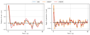
Figure 1: Performance of all three algorithms on inverted pendulum on cart. The task is to stabilise the system state at $x=0$ and $\theta=\pi$.

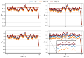
Figure 2: Performance of all three algorithms on spring mass damper. The dashed lines represent the solutions of the respective AREs, and the solid lines are the solutions obtained by running the EnKF algorithm.

Appendix A Proof of main results

Cost	$\frac{\partial p_{t}}{\partial t}$
SOC	$=p_{t}(\dot{\beta}_{t}+{\mathchoice{\genfrac{}{}{}{1}{1}{2}}{\genfrac{}{}{}{2}{1}{2}}{\genfrac{}{}{}{3}{1}{2}}{\genfrac{}{}{}{4}{1}{2}}}|c|^{2})-(\nabla p)^{\intercal}a+\frac{1}{2p_{t}}\nabla p_{t}^{\intercal}(\Sigma-D)\nabla p_{t}-\frac{1}{2}\mathrm{tr}(\Sigma\nabla^{2}p_{t})$
	$=p_{t}(h_{t}-\hat{h}_{t})-\nabla\cdot(p_{t}a)-\frac{1}{2}\nabla^{2}\cdot(Dp_{t})+\nabla\cdot(p_{t}\nabla\cdot D)$
RSC $\theta>0$	$=p_{t}(\dot{\beta}_{t}+\frac{\theta}{2}|c|^{2})-(\nabla p_{t})^{\intercal}a+\frac{1}{2p_{t}}(\nabla p_{t})^{\intercal}(2\Sigma-\frac{1}{\theta}D)\nabla p_{t}-\frac{1}{2}\mathrm{tr}(\Sigma\nabla^{2}p_{t})$
	$=p_{t}(h_{t}-\hat{h})-\nabla\cdot(p_{t}a)-\frac{1}{2}\nabla^{2}\cdot(p_{t}(\frac{1}{\theta}D-\Sigma))+\nabla\cdot(p_{t}\nabla\cdot(\frac{1}{\theta}D-\Sigma))$
RSC $\theta<0$	$=p_{t}(\dot{\beta}_{t}-\frac{\theta}{2}|c|^{2})-(\nabla p_{t})^{\intercal}a+\frac{1}{2\theta p_{t}}(\nabla p_{t})^{\intercal}D\nabla p_{t}-\frac{1}{2}\mathrm{tr}(\Sigma\nabla^{2}p_{t})$
	$=p_{t}(h-\hat{h})-\nabla\cdot(p_{t}a)-\frac{1}{2}\nabla^{2}\cdot(p_{t}(\Sigma-\frac{1}{\theta}D))+\nabla\cdot(p_{t}\nabla\cdot(\Sigma-\frac{1}{\theta}D))$

TABLE VI: PDE for density obtained from (6)

The PDE for $p_{t}(\cdot)$, defined in (6), are expressed in Table VI. Let $R_{\eta}$ denote the covariance of $\eta$, and define $D_{\eta}(z)\coloneqq b(z)R_{\eta}^{-1}b(z)^{\intercal}$. Then the Fokker Planck equation for the mean field system (8) reads

$$\frac{\partial\bar{p}_{t}}{\partial t} =-\nabla\cdot(\bar{p}_{t}(a+\mathcal{I}_{t}(\cdot;\bar{p}_{t})+\mathcal{C}_{t}(\cdot;\bar{p}_{t})))$$

$$\qquad-{\mathchoice{\genfrac{}{}{}{1}{1}{2}}{\genfrac{}{}{}{2}{1}{2}}{\genfrac{}{}{}{3}{1}{2}}{\genfrac{}{}{}{4}{1}{2}}}\nabla^{2}\cdot(p_{t}(D_{\eta}+\Sigma)).$$ (17)

Proof of Proposition 1: Substituting the appropriate vector fields from Table V into (17), we see that $p_{t}(\cdot)$ and $\bar{p}_{t}$ satisfy the same PDEs with the same terminal conditions. We used the following expressions to do the calculations

$$a^{\intercal}\nabla\bar{p}_{t} =\nabla\cdot(\bar{p}_{t}a)-\bar{p}_{t}\nabla\cdot a$$

$$\mathrm{tr}(\Sigma\nabla^{2}\bar{p}_{t}) =\nabla^{2}\cdot(\bar{p}_{t}\Sigma)-2\nabla\cdot(\bar{p}_{t}\nabla\cdot\Sigma)+\bar{p}_{t}\nabla^{2}\cdot\Sigma$$

$$\nabla^{2}\log\bar{p}_{t} =\frac{1}{\bar{p}_{t}}\nabla^{2}\bar{p}_{t}-\frac{1}{\bar{p}_{t}^{2}}\nabla\bar{p}_{t}\nabla\bar{p}_{t}^{\intercal},$$

$$\beta_{t} \coloneqq\int\bar{p}_{t}(z)\mathrm{d}z,\quad\hat{h}\coloneqq\int h(z)\bar{p}_{t}(z)\mathrm{d}z,$$

and since $\int\frac{\partial\bar{p}_{t}}{\partial t}\mathrm{d}z=0$ we have $\dot{\beta}_{t}=-\hat{h}$.

Expressions for LQ case: Since the system is LTI, we have $\nabla\cdot(\frac{1}{\theta}D-\Sigma)=0$, and $\nabla^{2}\cdot(\bar{p}_{t}\Sigma)=\mathrm{tr}(\Sigma\nabla^{2}\bar{p}_{t})$. We postulate that $\bar{p}_{t}=\mathcal{N}(n_{t},S_{t})$, with $n_{t}=0$ for all $0\leq t\leq T$ to verify that the expressions for $\mathcal{I}_{t},\mathcal{C}_{t}$ in Table IV satisfy (9). Now for any trial vector field $\omega_{t}(\cdot)$ we have

$$\nabla\cdot(\bar{p}_{t}\omega_{t})=\bar{p}_{t}\nabla\cdot\omega_{t}+\omega_{t}^{\intercal}(\nabla\bar{p}_{t}).$$

To begin we observe $\nabla\bar{p}_{t}=-\bar{p}_{t}S_{t}^{-1}(z-n_{t})$,

$$\nabla^{2}\bar{p}_{t}=-\bar{p}_{t}S_{t}^{-1}+\bar{p}_{t}S_{t}^{-1}(z-n_{t})(z-n_{t})^{\intercal}S_{t}^{-1},$$

$$\nabla\cdot(S_{t}C^{\intercal}C(z+n_{t}))=S_{t}C^{\intercal}C$$

$$\nabla\cdot(\Sigma S_{t}^{-1}(z-n_{t}))=\Sigma S_{t}^{-1}.$$

Moreover, since $\nabla^{2}\log\bar{p}_{t}=S_{t}^{-1}$, and $\nabla\cdot(Az)=\mathrm{tr}(A)$, we have that

$$h_{t}(z)=\begin{cases}{\mathchoice{\genfrac{}{}{}{1}{1}{2}}{\genfrac{}{}{}{2}{1}{2}}{\genfrac{}{}{}{3}{1}{2}}{\genfrac{}{}{}{4}{1}{2}}}|Cz|^{2}\,+\,(\text{function of }t\text{ only});&\text{LQG}\\ \vskip 5.0pt\cr\frac{|\theta|}{2}|Cz|^{2}\,+\,(\text{function of }t\text{ only});&\text{LEQG}\end{cases}$$

therefore,

$$\hat{h}_{t}=\begin{cases}{\mathchoice{\genfrac{}{}{}{1}{1}{2}}{\genfrac{}{}{}{2}{1}{2}}{\genfrac{}{}{}{3}{1}{2}}{\genfrac{}{}{}{4}{1}{2}}}\mathrm{tr}(C^{\intercal}C(S_{t}+n_{t}n_{t}^{\intercal}));&\text{LQG}\\ \vskip 5.0pt\cr\frac{|\theta|}{2}\mathrm{tr}(C^{\intercal}C(S_{t}+n_{t}n_{t}^{\intercal}));&\text{LEQG}\end{cases}$$

Substituting into (9) we see that the equations are indeed satisfied. The Gaussian hypothesis is also verified because the terminal condition of the mean-field process is Gaussian, and the equation for mean-field process becomes linear.

Proof of Proposition 2: substituting $\mathcal{C}_{t}\equiv 0$ and the corresponding expression for $D_{\eta}$ in (17), and using the simplifications stated above for the LQ case, we see that the Fokker Planck equation (17) matches the PDE for $p$ as given in Table VI.

References

• [1] A. A. Joshi, A. Taghvaei, P. G. Mehta, and S. P. Meyn, “Controlled interacting particle algorithms for simulation-based reinforcement learning,” Systems & Control Letters, vol. 170, p. 105392, 2022. [Online]. Available: https://www.sciencedirect.com/science/article/pii/S0167691122001694
• [2] W. H. Fleming and S. K. Mitter, “Optimal Control and Nonlinear Filtering for Nondegenerate Diffusion Processes,” Stochastics, vol. 8, no. 1, pp. 63–77, January 1982. [Online]. Available: https://doi.org/10.1080/17442508208833228
• [3] O. B. Hijab, “Minimum energy estimation,” Ph.D. dissertation, University of California, Berkeley, 1980.
• [4] R. E. Mortensen, “Maximum-likelihood recursive nonlinear filtering,” Journal of Optimization Theory and Applications, vol. 2, no. 6, pp. 386–394, Nov 1968. [Online]. Available: https://doi.org/10.1007/BF00925744
• [5] E. Todorov, “Linearly-solvable markov decision problems,” in Advances in Neural Information Processing Systems, B. Schölkopf, J. Platt, and T. Hoffman, Eds., vol. 19.   MIT Press, 2007. [Online]. Available: https://proceedings.neurips.cc/paper/2006/file/d806ca13ca3449af72a1ea5aedbed26a-Paper.pdf
• [6] H. J. Kappen, “Linear theory for control of nonlinear stochastic systems,” Phys. Rev. Lett., vol. 95, p. 200201, Nov 2005. [Online]. Available: https://link.aps.org/doi/10.1103/PhysRevLett.95.200201
• [7] ——, “Path integrals and symmetry breaking for optimal control theory,” Journal of Statistical Mechanics: Theory and Experiment, vol. 2005, no. 11, pp. P11 011–P11 011, nov 2005. [Online]. Available: https://doi.org/10.1088/1742-5468/2005/11/p11011
• [8] S. Vijayakumar, K. Rawlik, and M. Toussaint, “On stochastic optimal control and reinforcement learning by approximate inference,” in Robotics: Science and Systems VIII, N. Roy, P. Newman, and S. Srinivasa, Eds., 2013, pp. 353–360.
• [9] M. Toussaint, “Robot trajectory optimization using approximate inference,” in Proceedings of the 26th Annual International Conference on Machine Learning, ser. ICML ’09.   New York, NY, USA: Association for Computing Machinery, 2009, p. 1049–1056. [Online]. Available: https://doi.org/10.1145/1553374.1553508
• [10] C. Hoffmann and P. Rostalski, “Linear optimal control on factor graphs — a message passing perspective —,” IFAC-PapersOnLine, vol. 50, no. 1, pp. 6314–6319, 2017, 20th IFAC World Congress. [Online]. Available: https://www.sciencedirect.com/science/article/pii/S2405896317313800
• [11] S. Levine, “Reinforcement learning and control as probabilistic inference: Tutorial and review,” 2018.
• [12] J. B. Rawlings, D. Q. Mayne, M. Diehl et al., Model predictive control: theory, computation, and design.   Nob Hill Publishing Madison, WI, 2017, vol. 2.
• [13] D. Maoutsa and M. Opper, “Deterministic particle flows for constraining stochastic nonlinear systems,” Phys. Rev. Res., vol. 4, p. 043035, Oct 2022. [Online]. Available: https://link.aps.org/doi/10.1103/PhysRevResearch.4.043035
• [14] S. Reich, “Particle-based algorithm for stochastic optimal control,” 2024.
• [15] G. Evensen, Data Assimilation. The Ensemble Kalman Filter.   New York: Springer-Verlag, 2006.
• [16] H. Nagai, Risk-Sensitive Stochastic Control.   London: Springer London, 2013, pp. 1–9. [Online]. Available: https://doi.org/10.1007/978-1-4471-5102-9_233-1
• [17] Logarithmic Transformations and Risk Sensitivity.   New York, NY: Springer New York, 2006, pp. 227–259. [Online]. Available: https://doi.org/10.1007/0-387-31071-1_6
• [18] D. Jacobson, “Optimal stochastic linear systems with exponential performance criteria and their relation to deterministic differential games,” IEEE Transactions on Automatic Control, vol. 18, no. 2, pp. 124–131, 1973.
• [19] K. J. K. J. Astrom, Introduction to stochastic control theory, ser. Mathematics in science and engineering ; v. 70.   New York: Academic Press, 1970.
• [20] A. Bensoussan, Estimation and Control of Dynamical Systems, ser. Interdisciplinary Applied Mathematics.   Springer International Publishing, 2018. [Online]. Available: https://www.springer.com/gp/book/9783319754550
• [21] J. Doyle, “Guaranteed margins for lqg regulators,” IEEE Transactions on Automatic Control, vol. 23, no. 4, pp. 756–757, 1978.
• [22] P. Whittle, “Risk-sensitive linear/quadratic/gaussian control,” Advances in Applied Probability, vol. 13, no. 4, pp. 764–777, 1981. [Online]. Available: http://www.jstor.org/stable/1426972
• [23] W. H. Fleming, “Risk sensitive stochastic control and differential games,” Communications in Information & Systems, vol. 6, no. 3, pp. 161 – 177, 2006.
• [24] P. Whittle, “Risk sensitivity, a strangely pervasive concept,” Macroeconomic Dynamics, vol. 6, no. 1, p. 5–18, 2002.
• [25] T. Başar, “Robust designs through risk sensitivity: An overview,” Journal of Systems Science and Complexity, vol. 34, no. 5, pp. 1634–1665, Oct 2021. [Online]. Available: https://doi.org/10.1007/s11424-021-1242-6
• [26] A. Biswas and V. S. Borkar, “Ergodic risk-sensitive control—A survey,” Annual Reviews in Control, vol. 55, pp. 118–141, 2023. [Online]. Available: https://www.sciencedirect.com/science/article/pii/S1367578823000068
• [27] A. Lim and X. Y. Zhou, “A maximum principle for risk-sensitive control,” in 42nd IEEE International Conference on Decision and Control, vol. 6, 2003, pp. 5819–5824 Vol.6.
• [28] T. E. Duncan, “Linear-exponential-quadratic gaussian control,” IEEE Transactions on Automatic Control, vol. 58, no. 11, pp. 2910–2911, 2013.
• [29] M. R. James, “Asymptotic analysis of nonlinear stochastic risk-sensitive control and differential games,” Mathematics of Control, Signals and Systems, vol. 5, no. 4, pp. 401–417, Dec 1992. [Online]. Available: https://doi.org/10.1007/BF02134013
• [30] D. Nualart and É. Pardoux, “Stochastic calculus with anticipating integrands,” Probability Theory and Related Fields, vol. 78, no. 4, pp. 535–581, 1988.
• [31] R. W. Brockett, Finite dimensional linear systems.   SIAM, 2015.
• [32] T. Yang, R. Laugesen, P. Mehta, and S. Meyn, “Multivariable feedback particle filter,” Automatica, vol. 71, pp. 10–23, 2016. [Online]. Available: https://www.sciencedirect.com/science/article/pii/S000510981630142X
• [33] D. Maoutsa, S. Reich, and M. Opper, “Interacting particle solutions of fokker–planck equations through gradient–log–density estimation,” Entropy, vol. 22, no. 8, 2020. [Online]. Available: https://www.mdpi.com/1099-4300/22/8/802
• [34] J. W. Kim and P. G. Mehta, “An optimal control derivation of nonlinear smoothing equations,” in Advances in Dynamics, Optimization and Computation, O. Junge, O. Schütze, G. Froyland, S. Ober-Blöbaum, and K. Padberg-Gehle, Eds.   Cham: Springer International Publishing, 2020, pp. 295–311.