Fast and Accurate Relative Motion Tracking for Two Industrial Robots

Abstract

Industrial robotic applications such as spraying, welding, and additive manufacturing frequently require fast, accurate, and uniform motion along a 3D spatial curve. To increase process throughput, some manufacturers propose a dual-robot setup to overcome the speed limitation of a single robot. Industrial robot motion is programmed through waypoints connected by motion primitives (Cartesian linear and circular paths and linear joint paths at constant Cartesian speed). The actual robot motion is affected by the blending between these motion primitives and the pose of the robot (an outstretched/close to singularity pose tends to have larger path-tracking errors). Choosing the waypoints and the speed along each motion segment to achieve the performance requirement is challenging. At present, there is no automated solution, and laborious manual tuning by robot experts is needed to approach the desired performance. In this paper, we present a systematic three-step approach to designing and programming a dual-robot system to optimize system performance. The first step is to select the relative placement between the two robots based on the specified relative motion path. The second step is to select the relative waypoints and the motion primitives. The final step is to update the waypoints iteratively based on the actual relative motion. Waypoint iteration is first executed in simulation and then completed using the actual robots. For performance measures, we use the mean path speed subject to the relative position and orientation constraints and the path speed uniformity constraint. We have demonstrated the effectiveness of this method on two separate testbeds, consisting of ABB robots and FANUC robots, for two challenging test curves. The performance improvement over the current industrial practice baseline is over 300%. Compared to the optimized single-arm case that we have previously reported, the improvement is over 14%.

Keywords: Industrial Robot, Dual-Arm Coordination, Motion Primitive, Motion Optimization, Redundancy Resolution, Trajectory Tracking

I INTRODUCTION

Industrial robots are increasingly deployed in applications such as spray coating [1], arc welding [2], deep rolling [3], surface grinding [4], cold spraying [5], etc., where the tool center point (TCP) frame attached to the end effector needs to track complex geometric paths in both position and orientation. In most applications, the task performance is characterized by the motion speed (how long it takes to complete the task), motion uniformity (how much the speed varies along the path), and motion accuracy (the maximum position and orientation tracking errors along the path).

We have previously presented a systematic approach to optimizing the single 6-dof robot tracking a spatial curve tracking with motion primitives [6]. To further improve the performance (high traversal speed subject to tracking accuracy and motion uniformity requirements), some manufacturers are exploring dual-arm coordinated motion for relative spatial curve tracking, such as in the cold spray coating of the metal leading edge of a turbine blade [7]. A mock-up of the same operation in our lab and in simulation are shown in Fig. 1.

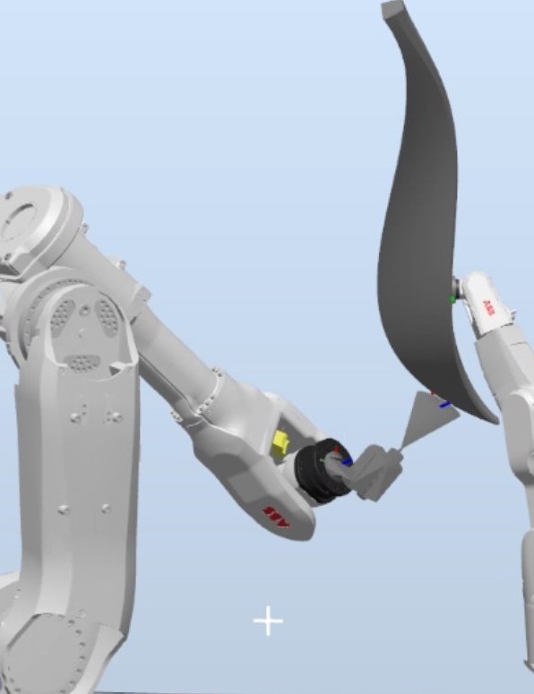
(a) Spraying in Simulation

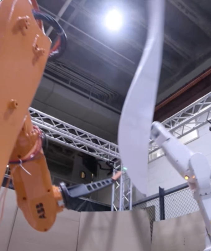
(b) Spraying Mock-up

Figure 1: Dual-arm turbine spraying mock-up in simulation and physical testbed.

To actually achieve the performance gain, there are many parameters that need to be tuned. We group these parameters as follows:

• System Configuration: A major difference between robotic vs. Computer Numerical Control (CNC) motion is that the robot motion constraints (end effector velocity and acceleration) are dependent on the robot pose. The relative configuration between the robots and the pose of each robot (out of the eight possible configurations) can significantly affect the achievable performance.

• Redundant Degrees of Freedom: Typical requirements for robot motion in deposition tasks involve 5 degree-of-freedom (dof), 3 for relative position and 2 for relative orientation (assuming a symmetric spraying pattern). When two 6-dof robots are used, there are 12-dof total, resulting in 7-dof kinematic redundancy to resolve.

• Waypoints and Motion Primitives: Industrial robot motion is specified by waypoints and motion primitives for the motion segments connecting the waypoints. There are three standard motion primitive types: moveL, moveC, moveJ (straight line or circle in the task space, straight line in the joint space). Higher density of waypoints approximates the path more closely, but the motion blending at the waypoints (to avoid acceleration constraints) compromises the speed uniformity and path following fidelity at the waypoints.

Current practice to select these parameters is largely manual, based on heuristics, experience, and trial-and-error iterations. The robots are placed so that both are roughly in the middle of their workspace (neither out-stretched nor tucked-in) throughout the relative motion path. For redundancy resolution, the relative motion is partitioned between the two robots based on their relative speed and size. For motion specification, there are offline programming software packages, e.g., [8, 9, 10], that convert the specified path to a dense set of TCP waypoints and then to a robot program for a given robot vendor, e.g., [11, 12, 13, 14, 15, 16]. Usually, only moveL is used to connect the motion segments. The actual robot motion from the execution of the programmed motion commands will depend on the motion primitives and their parameters (waypoint locations, commanded path speed along the motion segment, size of the blending zone between motion segments) and the pose of the robot, due to the robot joint servo controller behavior and the robot joint motion constraints (joint velocity and acceleration limits). For most industrial robots, robot controller and robot joint constraints are not known to the user. Therefore, programming a robot to achieve the desired performance is currently a time-consuming and largely manual exercise in tuning the motion primitive parameters and the result may be far from optimal.

In this paper, we present a systematic approach to generating a robot motion program to improve the relative tracking performance between two robots. This work extends the single-arm case [6] to the dual-arm scenario. The first step is to optimize the relative placement between the two robots using resolved motion control to track the specified relative motion. The actual robot control will be based on motion primitives, but the resolved motion control gives a good indication of advantageous relative robot placement subject to robot joint velocity and acceleration constraints. The second step is to achieve the best fit of the path with the minimum number of waypoints (blending between waypoints tends to degrade performance). As the actual robot motion will certainly deviate from the commanded motion, the final step is to update the waypoints iteratively based on the actual relative motion tracking error. This update will only be applied to the waypoints around the tracking error exceeding the accuracy constraint, and be based on the gradient of the error with respect to the nearby waypoints. Waypoint iteration is first applied to the robot simulator from the robot vendor. The results are then further refined using the actual robot tracking error.

Cycle time with quality assurance is the main performance assessment metric in practice. Therefore, as a quantitative performance measure, we use the mean path speed subject to the relative position and orientation and the path speed uniformity constraints. For dual-arm coordination, major robot vendors provide an internal synchronized multi-robot module, e.g., ABB Multimove [17], FANUC MultiArm [18] and Coordinated Motion [19], and MOTOMAN Coordinated Control Function [20]. We have developed drivers [21, 22, 23] for these industrial robot multi-arm controllers to command all 12 joints synchronously using the motion primitives. We have demonstrated the effectiveness of our method on a physical robot testbed consisting of an ABB IRB 6640 robot as the spraying robot and an ABB IRB 1200 robot holding the target curve, as shown in Fig. 1(a), with ABB RobotStudio as the simulation platform. We also applied the approach to FANUC M10iA robot (spraying arm) and LR Mate 200iD (target curve arm) in the FANUC simulation platform, RoboGuide. In all cases, the performance improves by over 14% compared with optimized single-arm results, and over 300% compared with baseline results in current industry practice.

II Problem Formulation

Given two robots, with robot 1 designated as the spraying and robot 2 as the arm holding the target curve, we denote the robot $i$ joint angle and angular velocities as $q^{(i)}$ and $\dot{q}^{(i)}$, $i=1,2$. Choose robot 1 tool $z$-axis, $e_{z}^{(1)}$, pointing in the spraying direction, and the TCP position, $p^{(1)}$ as the tip of the sprayer extended by a specified standoff distance in the $e_{z}^{(1)}$ direction. Choose the initial point on the curve as robot 2 TCP denoted by $p^{(2)}$ and tool $z$-axis, $e_{z}^{(2)}$, as the outward normal of the curve surface (as the curve is part of the surface of a part), and the tool $x$-axis, $e_{x}^{(2)}$, pointing in the curve tangent direction as shown in Fig. 2.

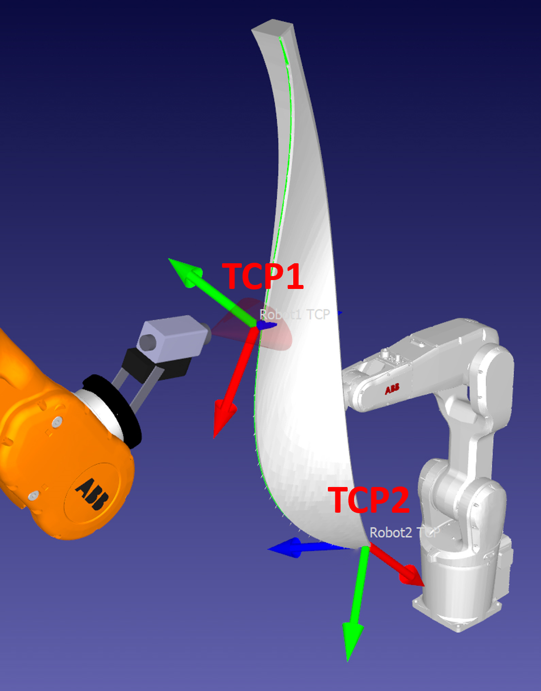
Figure 2: Spray Part, Curve, TCP frames and Tools.

Let $(f_{p}(q,T_{b}),f_{R}(q,T_{b}))$ denote the forward position kinematics mapping joint angle $q$ and base transform $T_{b}$ to the TCP position and orientation. Then $p^{(i)}=f_{p}(q^{(i)},T_{b}^{(i)})$, $R^{(i)}=f_{R}(q^{(i)},T_{b}^{(i)})$. Since only the relative base transform matters, we may set $T_{b}^{(1)}$ as the identity matrix, and will omit it in $f_{p}$ and $f_{R}$ for robot 1. For a given initial arm joint angle $q^{(1)}_{0}$ and $q^{(2)}_{0}$, the pose of the arm (one out of the eight possible choices) is determined if the arms do not cross singularity.

Denote the path length of the target curve from the start of the curve to a point on the curve by $\lambda$ and the total path length by $\lambda_{f}$. Since the target curve is rigidly held by robot 2 end effector, parameterize the curve in terms its position $p^{*}(\lambda)$ and outward surface normal $n^{*}(\lambda)$. The dual arm trajectory optimization problem may be stated as maximizing the constant relative path speed subject to the dual arm kinematics and robot joint velocity and acceleration constraints:
P1: Dual-Arm Trajectory Optimization
Given $\dot{\lambda}=\mu$, $\mu$ is a constant, $\lambda(0)=0$, $\lambda(t_{f})=\lambda_{f}$, $t_{f}=\lambda_{f}/\mu$. Find the configuration parameters $(q^{(1)}_{0},q^{(2)}_{0},T^{(2)}_{b})$ and robot joint velocities $(\dot{q}^{(1)}(\lambda),\dot{q}^{(2)}(\lambda))$, $\lambda\in[0,\lambda_{f}]$, to maximize $\mu$ subject to

$$p^{(1)}(\lambda)-p^{(2)}(\lambda)=R^{(2)}(\lambda)p^{*}(\lambda)$$ (1a)

$$e_{z}^{(1)}(\lambda)=-R^{(2)}(\lambda)n^{*}(\lambda)$$ (1b)

$$\left|{{\dot{q}}^{(i)}}\right|\preccurlyeq v_{\max}^{(i)},\quad\left|{\ddot{q}^{(i)}}\right|\preccurlyeq a_{\max}^{(i)},\quad i=1,2$$ (1c)

Note that $\dot{p}^{(i)}=J^{(i)}(q^{(i)})\dot{q}^{(i)}$, $p^{(i)}(\lambda)=f_{p}^{(i)}(q^{(i)}(\lambda),T_{b}^{(i)})$, $R^{(i)}(\lambda)=f_{R}^{(i)}(q^{(i)}(\lambda),T_{b}^{(i)})$. Path tracking constraints are captured in Eq. (1a)–(1b) for position and surface normal. Together it is a 5-dof constraint for the 12-dof joint velocity variables. Eq. (1c) are the robot joint velocity and acceleration limits, where $\preccurlyeq$ denotes elementwise inequality. We also assume there is an initial ramp up path, so $\dot{q}^{(i)}(0)$ may be nonzero. Since we require the perfect path following:

$$\dot{\lambda} =\frac{d\left\lVert p^{*}(\lambda)\right\rVert}{dt}=\frac{(p^{(1)}-p^{(2)})^{T}(\dot{p}^{(1)}-\dot{p}^{(2)})}{\left\lVert p^{(1)}-p^{(2)}\right\rVert}$$ (2)

$$=\frac{(p^{(1)}-p^{(2)})^{T}}{\left\lVert p^{(1)}-p^{(2)}\right\rVert}(J_{p}^{(1)}(q^{(1)})\dot{q}^{(1)}-J_{p}^{(2)}(q^{(2)})\dot{q}^{(2)}).$$

Then for each choice of the configuration parameters and robot joint velocities, there is a corresponding feasible region in the $(\lambda,\dot{\lambda})$ space corresponding to the constraints. The minimum of the infeasible region is the maximum allowed constant path speed as shown in Fig. 3. The goal of the optimization problem is then to find the parameters and robot joint trajectory so that the minimum of the infeasible region is as large as possible.

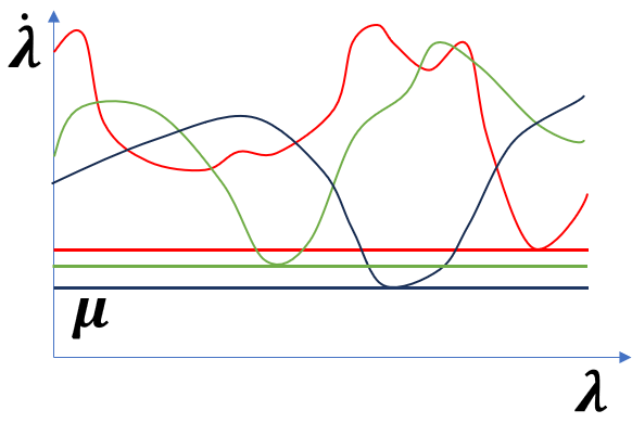
Figure 3: Infinite possible solutions for trajectory tracking with redundancies. Depending on different initial configurations, the $\dot{\lambda}$ profile varies, and we pick the solution with the largest $min(\dot{\lambda})$ along the trajectory and set $\mu$ as the commanded trajectory speed.

In practice, some tolerance of the constraints is acceptable. The optimization problem may be relaxed to the following form:
P2: Relaxed Dual-Arm Trajectory Optimization
Given $\dot{\lambda}=\mu(\lambda)$, $\lambda(0)=0$, $\lambda(t_{f})=\lambda_{f}$, $\int_{0}^{t_{f}}\dot{\lambda}(\tau)\,d\tau=\lambda_{f}$.
Find the configuration parameters $(q^{(1)}_{0},q^{(2)}_{0},T^{(2)}_{b})$ and robot joint velocities $(\dot{q}^{(1)}(\lambda),\dot{q}^{(2)}(\lambda))$, $\lambda\in[0,\lambda_{f}]$, to maximize $\mu_{avg}$, the mean of $\mu(\lambda)$ subject to

$$\sigma(\mu(\lambda))\leq\epsilon_{\mu}\mu_{avg}$$ (3a)

$$\left\lVert p^{(1)}(\lambda)-p^{(2)}(\lambda)-R^{(2)}(\lambda)p^{*}(\lambda)\right\rVert\leq\epsilon_{p}$$ (3b)

$$\left|{\angle(e_{z}{{{}^{(1)}}}(\lambda),-R^{(2)}(\lambda)n^{*}(\lambda))}\right|\leq\epsilon_{n}$$ (3c)

and joint velocity and acceleration bounds in (1c)

The path speed standard deviation is allowed to vary by $\epsilon_{\mu}$ (usually specified as a percentage) about the average path speed. The position and normal tracking errors are allowed to vary by $\epsilon_{p}$ and $\epsilon_{n}$, respectively. In this study, we choose $\epsilon_{\mu}=5\%$, $\epsilon_{p}=0.5mm$, $\epsilon_{n}=3^{\circ}$, based on typical industry specification for cold spray coating of turbine blades.

For industrial robots, there is an additional restriction. The path speed $\mu(\lambda)$ cannot be arbitrarily specified at each point on the path. Instead, robot motion is specified in terms of waypoints connected by motion segments. As shown in Fig. 4, every industrial robot provides three motion primitives for the motion segments:

• moveL: The robot motion is given by the straight line motion between the adjacent waypoints specified in the tool frames: $(p_{k},\beta_{k})$ and $(p_{k+1},\beta_{k+1})$, where $\beta$ is typically the angle-axis product of the tool orientation though other parameterization (e.g., vector quaternion for ABB).

• moveC: The position portion of the robot motion is given by a circular arc in the tool frame. The orientation portion is given by straight line interpolation in a specified parameterization.

• moveJ: The robot motion is given by the straight line motion in the joint space between the adjacent waypoints specified in the joint space: $q_{k}$ and $q_{k+1}$.

Even though the motion primitives are universal, there are subtle differences from vendors to vendors, including target types (joint position or Cartesian pose with specified configuration), blending region specification (in radius or percentage) and speed (percentage or $rad/s$ or $mm/s$). These vendor-specific arguments are taken care of in our robot drivers [21, 22, 23] to parse into vendor-specific programming scripts, such that the optimization algorithm can interface directly.

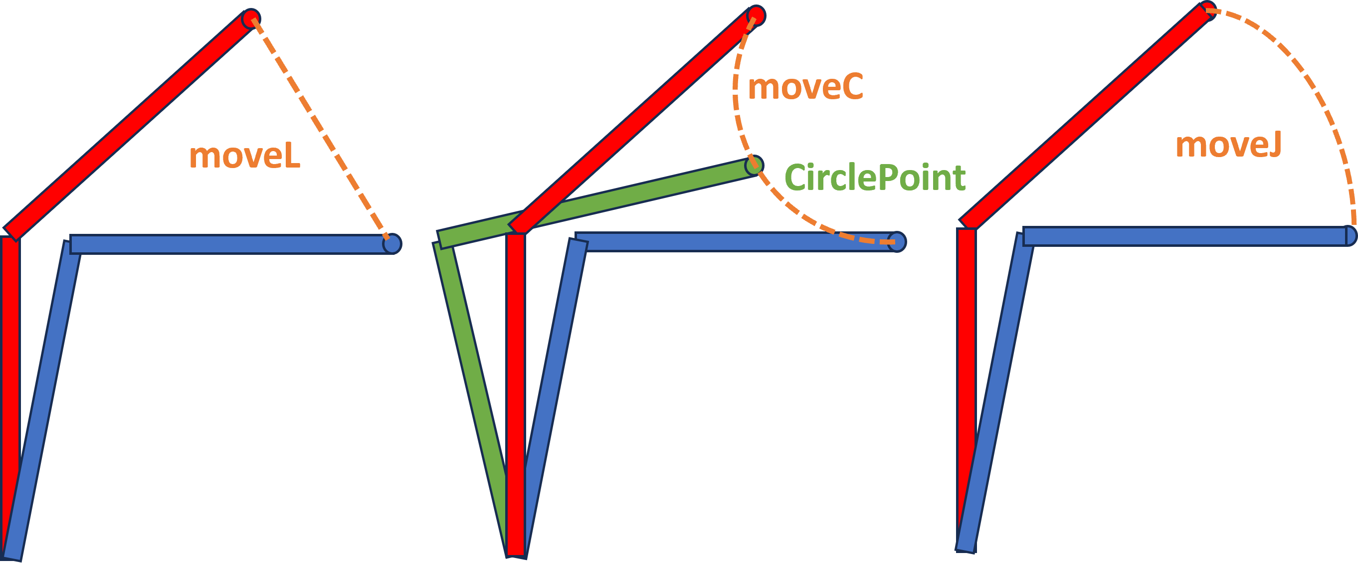
Figure 4: Three types of robot motion primitives. moveL: linear in Cartesian Space; moveC: circular arc in Cartesian space, defined by start, end and a circlepoint; moveJ: linear in joint space.

A motion program for an industrial controller consists of a set of waypoints, indexed as $k=1,\ldots,K$ (with an initial condition as $k=0$), $K$ motion primitives connecting the waypoints, and the Cartesian path speed in the motion segment. To avoid high acceleration at the waypoints, one can specify a blending region as shown in Fig. 5. Different vendors may handle blending differently to smooth out the trajectory, such as blending in joint space directly or in Cartesian space.

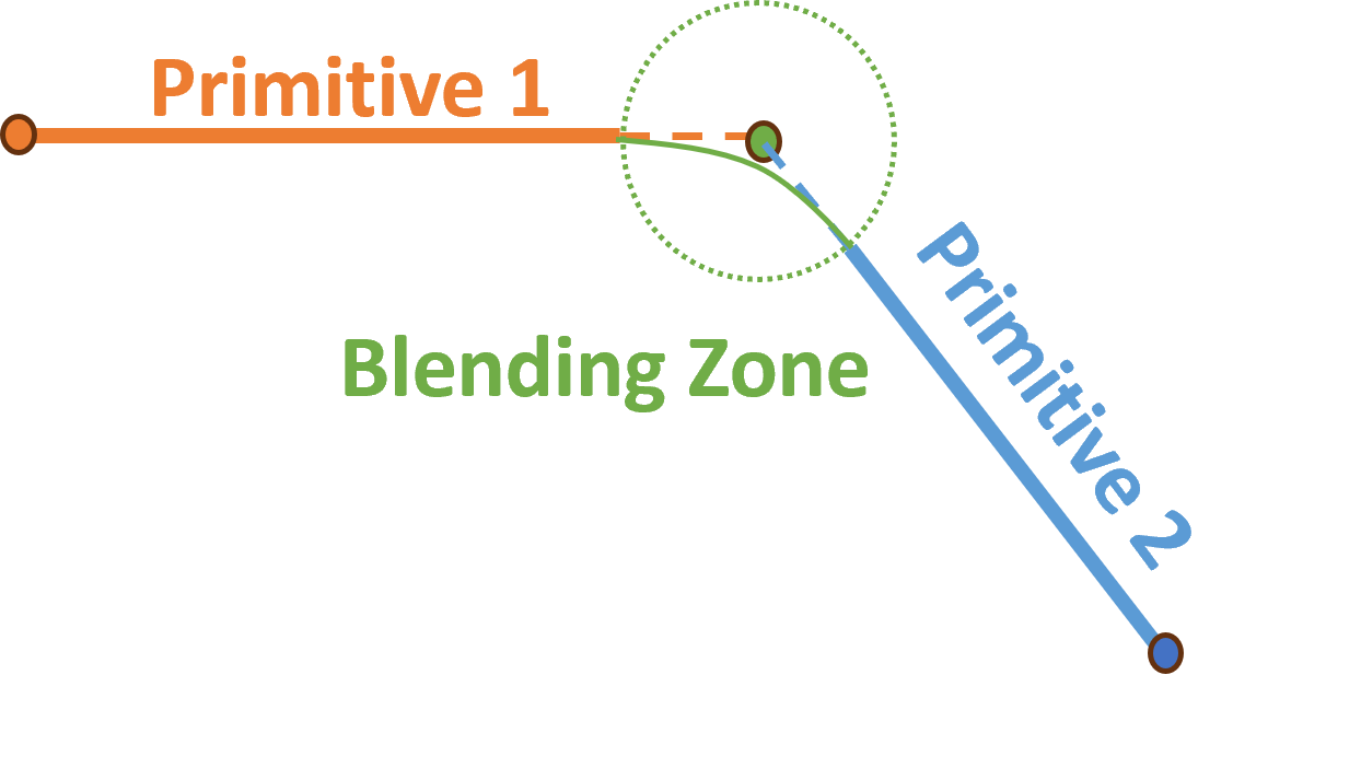
Figure 5: Blending between Two Motion Primitives.

Robot vendors use proprietary blending strategies and low-level motion control algorithms, so the exact behavior of the robot motion is not known a priori. In general, a large blending region tends to have smoother motion (path velocity is more uniform) but a larger error at the waypoint (distance between the motion and the waypoint).

For dual-arm motion, one can specify the waypoints for both robots and they are synchronized based on the slower of the two path speeds so both robots can execute the motion segment in the same time period. The blending zone for dual-arm in synchronized motion is identical to the single-arm case, embedded in the motion primitive commands.

III Solution Approach

III-A Summary Of Approach

We decompose the problem into multiple steps. The first step is to optimize the system configuration based on the idealized optimization problem. The second step is to approximate the optimal solution using the robot motion program consisting of motion primitives. The final step is to adjust the waypoints in the motion program to ensure the constraints are satisfied. These steps are described further below:

• System Configuration Optimization: For a given system configuration $(q^{(1)}_{0},q^{(2)}_{0},T_{b}^{(2)})$, we use dual-arm resolved motion control to find the entire joint space trajectory under constraints (1a)–(1c). A speed estimation model is used to find the maximum constant $\mu$, we then use differential evolution to find the best system configuration to maximize $\mu$.

• Waypoint Optimization: The solution in step 1 is not directly realizable using industrial robot motion programs. Instead, we will approximate the target curve in terms of motion primitives to within a specified tolerance while using the smallest number of waypoints. The reason is that waypoints tend to compromise performance due to the need to blend motion segments. We apply greedy search in this step by choosing the best motion primitive type for each motion segment. We then use the simulator from the robot vendor to check the path constraints (1a)–(1b). The robot velocity and acceleration constraints are typically already enforced in the simulator. The path speed is then lowered from step 1 until the path constraints and speed uniformity constraint (3a) are satisfied.

• Waypoint Iteration: The final step is to adjust the waypoints directly to improve the path constraints, and continue to increase the path speed, until the path or speed uniformity constraints can no longer be satisfied. This step is performed first in simulation and continued with the physical robots if available.

III-B System Configuration Optimization

We first solve the feasibility problem: Given a specified path velocity $\mu$ and system configuration parameters $\theta=(q^{(1)}_{0},q^{(2)}_{0},T_{b}^{(2)})$, find $(\dot{q}^{(1)},\dot{q}^{(2)})$ to satisfy the constraints in P1 (1a)–(1c). Differentiate (1a)–(1b) to convert into equations involve ${\dot{q}}^{(i)}$:

$$J^{(1)}_{p}{\dot{q}}^{(1)}-J^{(2)}_{p}{\dot{q}}^{(2)}+(R^{(2)}p^{*})^{\times}J^{(2)}_{\omega}{\dot{q}}^{(2)} =R^{(2)}{p^{*}}^{\prime}\mu$$ (4a)

$${e_{z}^{(1)}}^{\times}J_{\omega}^{(1)}{\dot{q}}^{(1)}+(R^{(2)}n^{*})^{\times}J^{(2)}_{\omega}{\dot{q}}^{(2)} =R^{(2)}{n^{*}}^{\prime}\mu$$ (4b)

where ($J^{(i)}_{p}$,$J^{(i)}_{\omega})$) are the position and orientation portion of the Jacobian matrix of Robot $i$, $({p^{*}}^{\prime},{n^{*}}^{\prime})$ denote the derivative of $(p^{*},n^{*})$ with respect to $\lambda$, and ^× denote the cross product operation. We use the resolved motion controller [24] that enforces trajectory tracking and joint motion constraints using all robot joints (thus achieving redundancy resolution at the same time). This is based on the constrained least square solution (posed as a quadratic programming, QP, problem):
P3: Dual-Arm Resolved Motion Control
At each $(q^{(1)},q^{(2)})$, solve $(\delta q^{(1)},\delta q^{(2)})$ from the following quadratic program:

$$\min_{\delta q}\left\lVert\bar{J}\delta q-\nu^{*}\right\rVert^{2}+\left\lVert\delta q\right\rVert_{W}^{2}$$ (5a)

 subject to

$$q_{\min}\preccurlyeq q^{(i)}_{k-1}+\delta q^{(i)}\preccurlyeq q_{\max},\,\,i=1,2$$ (5b)

where $\bar{J}\!\!=\!\!\left[\begin{array}[]{cc}\bar{J}^{(1)}(q^{(1)})&\bar{J}^{(2)}(q^{(2)})\end{array}\right]$, $\delta q$ is the stacked vector of $(\delta q^{(1)},\delta q^{(2)})$, $W$ is a weighting matrix, and

$$\bar{J}^{(1)}(q^{(1)}) =\left[\begin{array}[]{c}J^{(1)}_{p}\\ {e_{z}^{(1)}}^{\times}J^{(1)}_{\omega}\end{array}\right]$$ (6c)

$$\bar{J}^{(2)}(q^{(2)}) =\left[\begin{array}[]{c}-J^{(2)}_{p}+(R^{(2)}p^{*})^{\times}J^{(2)}_{\omega}\\ (R^{(2)}n^{*})^{\times}J^{(2)}_{\omega}\end{array}\right]$$ (6f)

$$\nu^{*} =\left[\begin{array}[]{c}R^{(2)}{p^{*}}^{\prime}\mu\\ R^{(2)}{n^{*}}^{\prime}\mu\end{array}\right]$$ (6i)

For all points on the curve, the QP formulation above will generate the corresponding 12 joint angles (if feasible). For the given trajectory for both arms, it is possible to estimate the maximum relative traversal speed based on joint velocity and acceleration constraints.

Industrial robot vendors usually provide joint velocity limits in the data sheets, e.g., [25, 26], but the acceleration limit is undisclosed due to the torque limit and dependence on the robot dynamics, load, and robot configuration. We have used an experimental procedure to determine the robot acceleration limit in various poses. Continuous joint positions are discretized linearly with a resolution of 0.3 $rad$, and at each discrete joint configuration, we command the robot to execute back-and-forth oscillation with maximum commanded speed. The acceleration limit is derived from the recorded joint trajectory, forming a dictionary that maps this configuration to the acceleration limit. To determine the acceleration limit at a given configuration, we find use the near-neighbor table lookup.

In the single-arm case [6], we described finding the joint acceleration of ABB6640. The acceleration identification routine is available in open-source on our GitHub repository [27] and tested on multiple robots including ABB6640, ABB1200 and Motoman MA2010. The joint acceleration limits are stored as a lookup table dependent on $(q_{2},q_{3})$.

ABB 6640	1	2	3	4	5	6
$v_{max}$ ($rad/s$)	1.745	1.571	1.571	3.316	2.443	3.316
$a_{max}$ ($rad/s^{2}$)	*	*	*	42.5	36.8	50.5
ABB 1200	1	2	3	4	5	6
$v_{max}$ ($rad/s$)	5.027	4.189	5.184	6.981	7.069	10.472
$a_{max}$ ($rad/s^{2}$)	*	*	*	108.2	145.4	153.5

TABLE I: ABB IRB 6640 and IRB 1200 joint velocity and acceleration limits. * denotes configuration dependent, see [27] for details.

With the estimated traversal speed given joint constraints, we next apply the differential evolution algorithm [28] to find the global optimized configuration with maximum $\mu$ (constant relative path traversal speed). Differential evolution is a global optimization evolution algorithm that involves mutation (generating new solutions by combining existing ones), crossover (mixing mutant solutions with current solutions), and selection (choosing the better solution for the next generation). The initial guess is the single-arm baseline, in which robot 2 holds the part statically. In cases such as robots nearing singularity or too far apart where the algorithm cannot find a solution, the path speed $\mu$ will be 0.

In our testbed, robot 1 is positioned flush on the floor and robot 2 is mounted on a mobile pedestal. Hence, the relative pose of $T_{b}^{(2)}$ is an $SE(2)$ transformation (3 parameters: two distances and an angle). The target trajectory is mounted close to the part center of mass so as to minimize the torque generated on the robot wrist. Together with $(q^{(1)}_{0},q^{(2)}_{0})$, there are 15 parameters to optimize in this step. The optimized dual-arm and single-arm system configurations for a sample turbine blade leading edge are shown in Fig. 6.

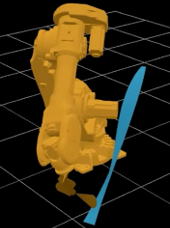
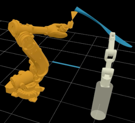
Figure 6: Optimized configuration for the single-arm case [6] vs. the dual-arm case in this paper.

The solution of Problem P3 used in differential evolution also yields the complete robot motion. For the two test curves used in our dual-arm testbed, discussed in Section IV-A, the maximum relative traversal speed, $\mu$, during the differential evolution optimization is shown in Fig. 7. The maximum number of iterations is set to 3000. The optimal path speeds for the two test curves are 1332.22 $mm/s$ and 3589.87 $mm/s$, respectively. Due to the unknown vendor-specific controller behaviors such as blending strategy and inner loop control settings, such high speeds are likely not achievable. We will discuss the implementation on the physical testbed in Section IV-C.

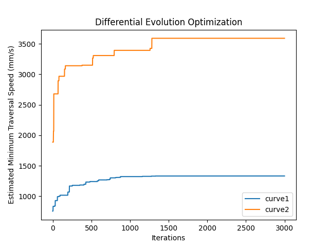
Figure 7: Differential evolution optimization progression for the estimated path traversal speed $\mu$ for the two test curves in Section IV-A. The final outputs are the complete robot joint trajectories and the robot base relative pose.

III-C Motion Primitive Planning with Greedy Fitting

The solution of Problem P3 will provide a feasible trajectory. However, it cannot be directly implemented using standard industry robot controllers as discussed in Section III-A. Current industry practice involves using moveL to interpolate the robot trajectory. While it’s possible to densely interpolate the trajectory directly with moveL or moveJ to achieve the closest motion primitive command, robot controllers will prevent close waypoints programming due to various reasons including overlapping blending zone, infeasible corner path, or a hard stop at certain waypoints with failed/interference blending. Furthermore, segments blending also compromise performance as shown in Fig. 8, and different vendors have different blending strategies. Therefore, we want to use the smallest number of waypoints with all three motion primitives that can fit a given curve.

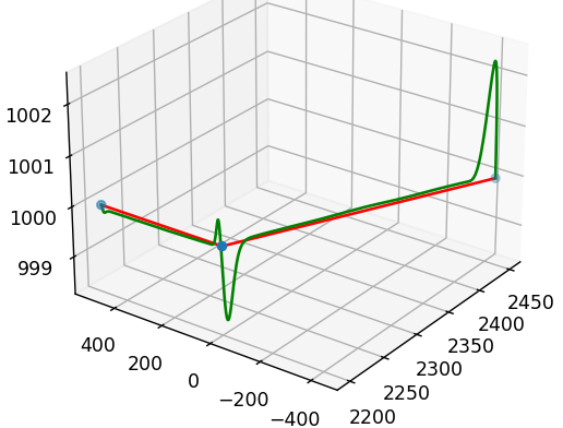
(a) Two moveL blending

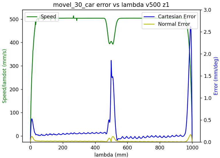
(b) Segment Blending Performance

Figure 8: ABB6640 30^∘ slope moveL blending at 500 $mm/s$ and blending zone of 1 $mm$. The blending in joint trajectory causes out-of-plane motion with large Cartesian error, and speed slows down.

In [6], we introduced the greedy fitting algorithm for the single-arm trajectory planning case. Motion primitive trajectory greedy fitting starts at the initial point and looks for the longest possible segment under the specified accuracy threshold with moveL/moveC/moveJ with unconstrained regression using bisection search. This step continues on the subsequent trajectory with continuity constraints.

For multi-robot control, there are various ways to command the robots. Similar to a single-arm control, it is possible to set up our drivers on two socket-connected computers talking to two individual IRC5 controllers respectively, or set up the drivers on the same computer as a centralized control computer. Both ways are feasible for slow-motion applications with more accuracy tolerance. However, for high-speed and high-accuracy requirements, we decided to take advantage of the vendor-proprietary controller, Multimove by ABB [17], MultiArm by FANUC [18] and Coordinated Control Function by Motoman [20] to achieve a low-level synchronized clock. Therefore, dual-arm motion command consists of two sets of motion primitives with shared waypoint indexing, meaning the motion of the two robots will be synchronized to reach the individual commanded waypoint at the same time.

For dual-arm applications, the greedy fitting algorithm is modified as shown in Fig. 9. Each robot has its own trajectory, and moveL/moveC/moveJ regression is performed on its Cartesian/joint space trajectory. Starting from the initial point, the greedy fitting performs unconstrained moveL/moveJ/moveC regression for robot 1 and robot 2 trajectories respectively. But the threshold is checked based on relative trajectory error, meaning the fitted motion primitive segment for robot 1 and robot 2 will be converted in robot 2’s TCP frame and calculates the tracking error to the original curve segment. Again we use bisection search to identify the furthest shared waypoint index, such that the relative error is under the specified threshold. And this process continues on both robot arm’s subsequent trajectories. The output motion primitive trajectory is further extended at the first and last motion segments for robots to accelerate/decelerate, to avoid the error introduced by acceleration/deceleration as shown in Fig. 8 and maintain a more consistent speed.

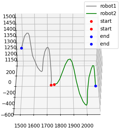
(a) Dual arm Cartesian trajectories.

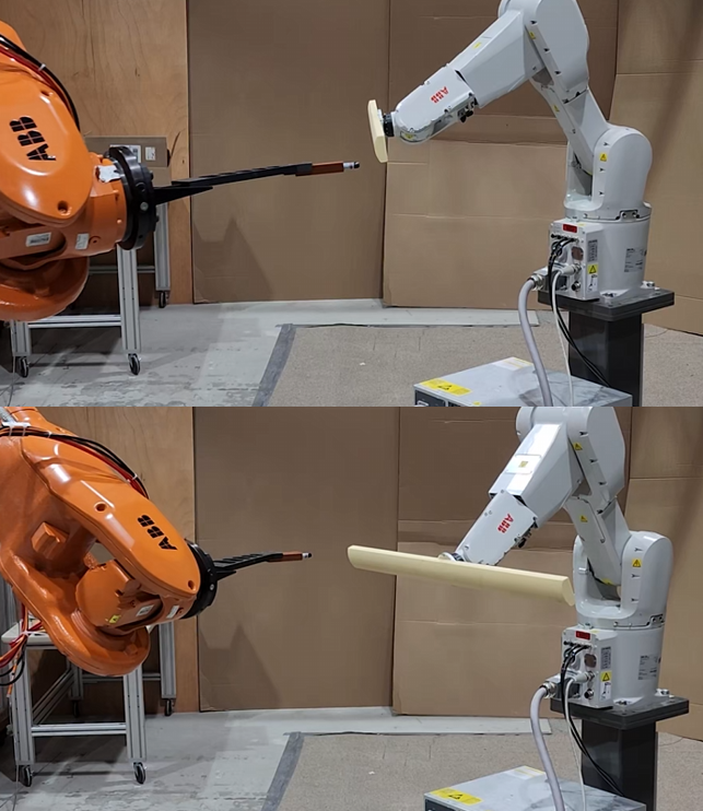
(b) Start and end poses of curve1.

Figure 9: Dual arm Greedy Fitting on curve 1: each robot has its own fitted motion primitive sequences. Starting from the red initial point, each pair motion segment is executed synchronously and finally arrives at the blue end point.

III-D Waypoint Adjustment

The waypoints and motion primitives from Section III-C together with the optimized path speed $\mu$ from Section III-B may be incorporated into the robot motion program and applied to the robot. However, invariably, the performance specification (3a) –(3c) will not be satisfied. This is caused by the effect of speed variation due to blending and the inherent performance limitation of the robot (velocity and acceleration limits) and robot controller. This performance degradation is dependent on the robot payload and configuration and is not possible to predict accurately without additional information from the robot vendor.

We apply an iterative approach to adjust the waypoints in the motion program based on the measured tracking error, first in simulation and then from physical robots, to improve the tracking accuracy. For each path speed $\dot{\lambda}=\mu$, we use waypoint iteration to reduce the tracking error. The path speed $\mu$ is reduced until all constraints (3a)–(3c) are satisfied.

From the single-arm setup, we have developed a proportional adjustment strategy based on reinforcement learning derived policy [29], where the all waypoints are adjusted in the direction of the tracking error vector. This strategy reduces the tracking error but may not meet the accuracy requirement. We follow up with a multi-peak gradient descent approach to adjust only waypoints with large tracking errors, using the gradient with respect to the waypoints and their immediate neighbors calculated based on an assumed blending using cubic splines. This process is summarized below:

• Proportional Adjustment: Adjust all waypoints for both robots in the relative error direction. For the $k$th waypoint and $i$th robot,

  $$p^{(1)}_{k}\leftarrow p^{(1)}_{k}-\gamma{e_{p}}_{k},\,\,\,p^{(2)}_{k}\leftarrow p^{(2)}_{k}+\gamma{e_{p}}_{k}$$ (7)

  $$R^{(1)}_{k}\!\!\leftarrow{\sf R}(e^{\perp}_{k},\gamma\theta_{k})R^{(1)}_{k},\,R^{(2)}_{k}\!\!\leftarrow{\sf R}(e^{\perp}_{k},-\gamma\theta_{k})R^{(2)}_{k}$$

  where $e_{p}$ is the position error from (3b), $\theta$ is the angular error from (3c):

  $$e_{p}={p^{(1)}-p^{(2)}-R^{(2)}p^{*}},\,\theta=\!\!{\angle(e_{z}{{{}^{(1)}}},-R^{(2)}n^{*})}$$ (8)

  $e^{\perp}$ is the normalized $e_{z}^{{(1)}^{\times}}R^{(2)}p^{*}$, ${\sf R}$ denotes the rotation matrix for a given axis and angle, $\gamma$ is the step size, $p^{*}_{k}$ is the point on the specified curve closest to $p_{k}$.

• Multi-peak Gradient Descent: After the proportional adjustment no longer reduces the worst case tracking error, we target error peaks in the region where error exceeds the tolerance. Let $p_{peak}$ be a peak error point on the trajectory. Define its error as ${p}_{err}={p}_{peak}-{p}_{peak}^{*}$, where ${p}_{peak}^{*}$ is the closest point on the desired relative trajectory. Identify the closest 3 waypoints in the relative commanded trajectory, call them ${p}_{wp_{i}}$, $i=1,\ldots,3$, corresponding to two sets of synchronized waypoints ${p}^{(1)}_{wp_{i}},{p}^{(2)}_{wp_{i}}$, for each arm. Define ${{p}^{\prime}_{peak}}$ as the closest point to ${p}_{peak}$ in a cubic spline interpolated predicted trajectory. Then calculate the gradient numerically $\frac{\delta{{p}^{\prime}_{peak}}}{\delta{{p}_{wp}}_{i}}$, which is an estimate of the actual error gradient on the executed trajectory. We can then estimate the error gradient $\frac{\delta e_{p}}{\delta{p_{wp}}_{i}}$ numerically, and use it to update the waypoints by gradient descent with adaptive step size. The same scheme is used for the orientation waypoint adjustment.

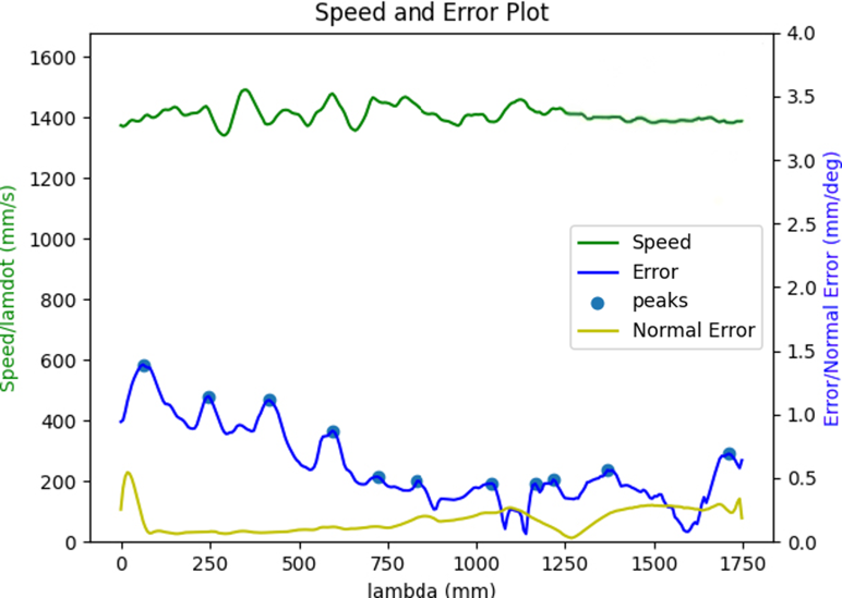
(a) Execution results with initial waypoints

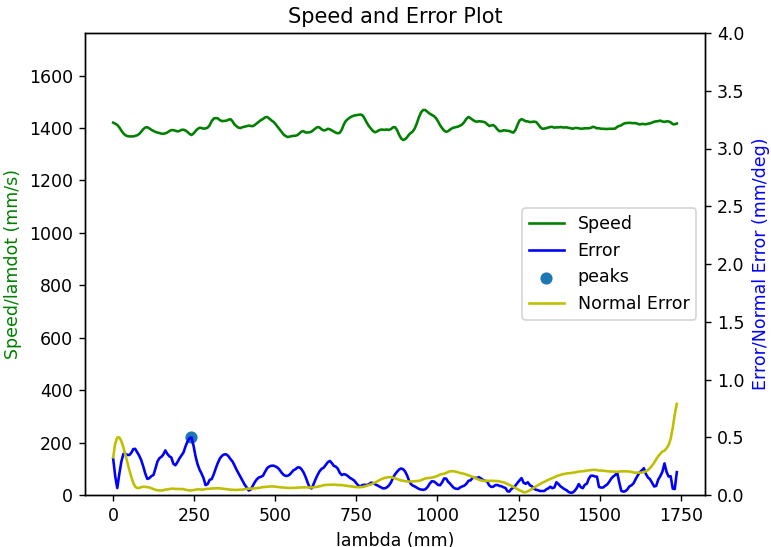
(b) Results with updated waypoints after five iterations

Figure 10: Execution results comparison (path speed, position error, normal error) initial waypoints vs. waypoints after five iterations. Peak position errors beyond the 0.5 $mm$ threshold are highlighted.

Fig. 10 shows the waypoint update progress for the test curve 2 on the physical robot trajectory execution, with the initial execution command from the best simulation using the robot vendor simulator. After five iterations, the relative tracking error with updated waypoint command is below the 0.5 $mm$ requirement.

IV Implementation and Evaluation

IV-A Test curves and Baseline

Based on industry needs, we choose two representative test curves as shown in Fig. 11(a) to evaluate our algorithms. Curve 1 is a multi-frequency spatial sinusoidal curve on a parabolic surface. This curve is representative of a high curvature spatial curve. Curve 2, shown in Fig. 11(b), is extracted from the leading edge of a generic fan blade model, which is a typical case for cold spraying applications in industry.

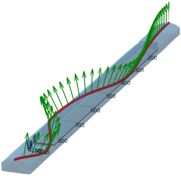
(a) Curve 1: frequency-changing sinusoidal curve on a parabolic surface.

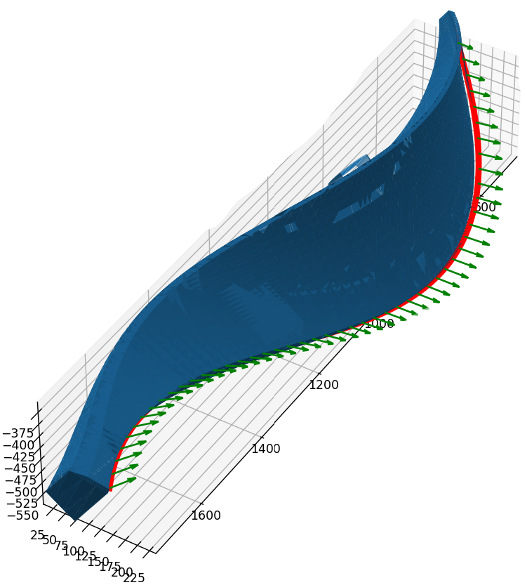
(b) Curve 2: generic Fan Blade leading edge curve.

Figure 11: Representative two 5-dof spatial curves.

Based on the current industry practice, we developed a baseline approach for a single arm tracking a stationary cure as a benchmark [6]. The target curve is positioned at the center of the robot workspace to avoid singularities. The redundant tool-$z$ orientation is addressed by aligning the tool $x$-axis with the motion trajectory. The selection of the robot arm pose is chosen by maximizing the manipulability. This baseline utilizes equally spaced moveL segments to interpolate the trajectory. The performance is determined by identifying the maximum allowable path speed that meets the criteria for traversal speed consistency and tracking accuracy specified in Section II. This approach will also serve as the baseline for the dual-arm case, with the second arm remaining stationary.

IV-B Simulation and Physical Setup

Dual-arm coordination with high precision requires a synchronized clock for both arms. We used MultiMove Slave Drive Module [17] with IRC5 controller [30] with RobotWare 6.13 to drive both ABB arms in our testbed synchronously as shown in Fig. 12.

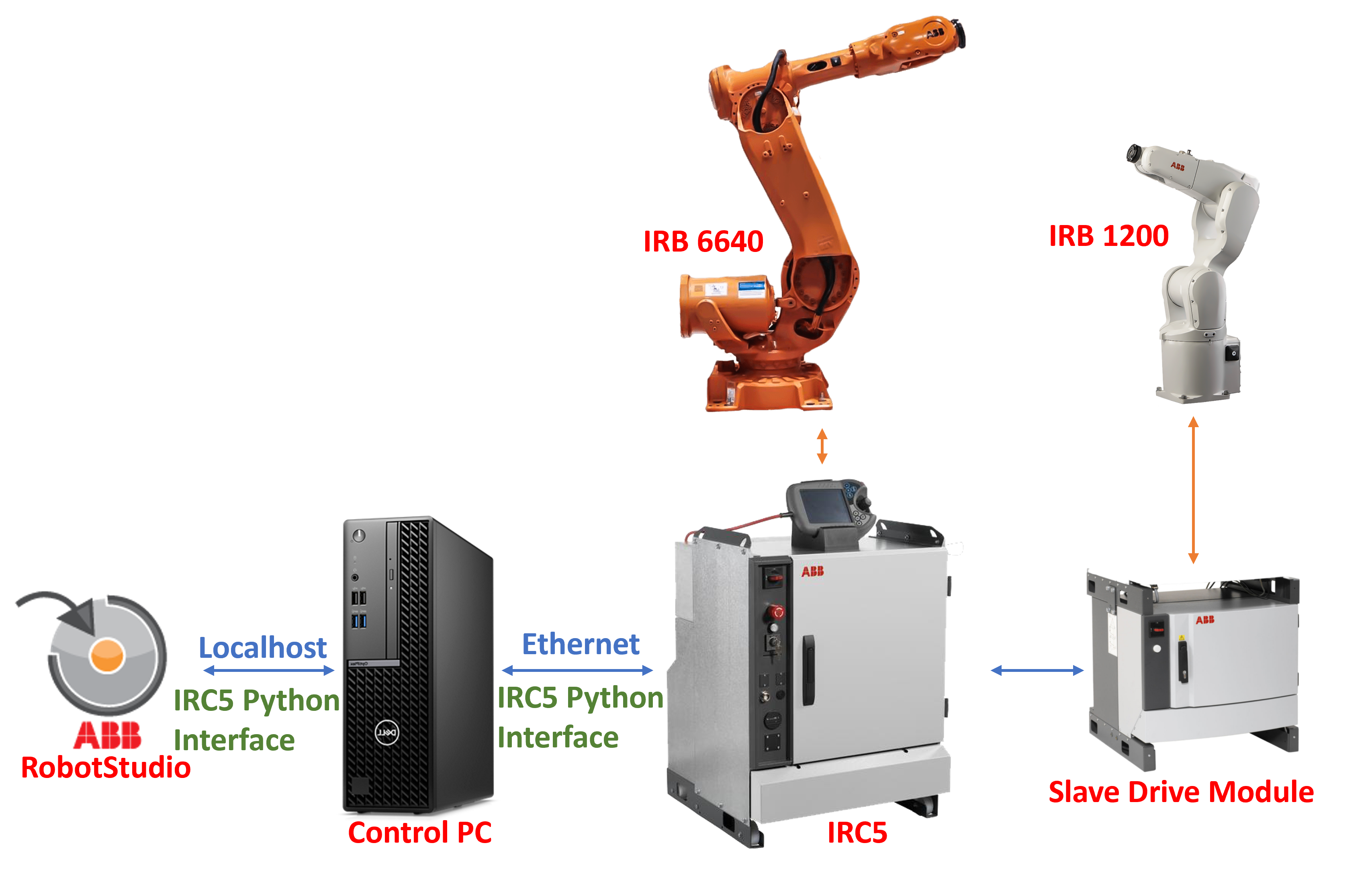
Figure 12: ABB Multimove setup for dual-arm control with the slave drive module. The control PC talks to IRC5 controller through UDP with our Python interface.

We have developed a Python interface [21] to the IRC5 controller and RobotStudio virtual controller [31] to execute motion commands directly. For all motion commands, we start with a blending zone of 10 $mm$ and gradually increase it until the speed profile converges such that the robot does not slow down around waypoints due to blending.

Fig. 1 shows the experiment setup for Curve 2, with the ABB6640 robot holding a mock spray gun and the ABB1200 robot holding the part to be machined. The joint trajectory is recorded through the robot controller at 250 Hz for all 12 joints. Robot forward kinematics is used to compute the TCP locations and the relative trajectory.

According to the manuals of ABB6640 and ABB1200, the path repeatability is up to 1.06 $mm$ [25] and 0.07 $mm$ [26] respectively. Therefore, we run the robot 5 times for each set of the motion primitive commands and take the interpolated average of 5 recorded trajectories as the execution trajectory.

IV-C Results

We applied our methodology using both RobotStudio simulation and the physical robot, and compare with the baseline, optimized single-arm approach as in [6]. The results are summarized below.

Curve 1	$max\,\,e_{p}$	$max\,\theta$	$\mu_{avg}$	$\sigma(\mu)/\mu_{avg}$
	mm	deg	mm/s	%
Baseline (sim)	0.49	0.18	124.01	0.82
Baseline (real)	0.46	0.21	103.11	0.82
Single Opt (sim)	0.48	0.57	399.81	1.62
Single Opt (real)	0.41	0.33	395.72	2.41
Dual Opt (sim)	0.42	1.49	550.73	4.13
Dual Opt (real)	0.41	2.29	451.52	3.74

Curve 2	$max\,\,e_{p}$	$max\,\theta$	$\mu_{avg}$	$\sigma(\mu)/\mu_{avg}$
Baseline (sim)	0.42	0.26	406.10	0.23
Baseline (real)	0.47	0.28	299.97	0.79
Single Opt (sim)	0.42	1.09	1207.45	0.95
Single Opt (real)	0.46	1.15	1197.43	1.11
Dual Opt (sim)	0.47	0.69	1705.26	1.10
Dual Opt (real)	0.50	0.80	1404.87	1.52

TABLE II: Results for RobotStudio Simulation and Physical Robot Experiments. $\mu_{avg}$ denotes average path speed, $\sigma(\mu)$ denotes standard deviation of speed along path. Baseline: Current industry practice. Single Opt: Results after optimization with single-arm (ABB6640) [6] Dual Opt: Results for using approach in this paper for the dual-arm system of ABB6640 and ABB1200.

The final optimized dual-arm results show 344% (sim) 337% (real) speed increase for Curve 1 and 319% (sim) and 368% (real) speed increase for Curve 2 over baseline while keeping the tracking accuracy within the requirement. The dual-arm results also show 38% (sim) 14% (real) speed increase for Curve 1 and 41% (sim) and 17% (real) speed increase for Curve 2 over single-arm optimized results. Since we used a much smaller robot as the second arm, the dual-arm results are not significantly improved over the optimized single-arm case. Since both robots are running on the shared master controller (IRC5), faster commanded speed will throw Corner Path Failure error [12] from motion segment blending, which prevents the robots from achieving their theoretical performance. We are also seeing the performance drop in reality over simulation. However, this systematic approach is applicable and optimized to all 5-dof trajectory traversal applications with dual-arm configuration.

IV-D Implementation for Dual-arm FANUC Robots

To demonstrate the applicability of the proposed methodology to other industrial robots, we evaluate the approach on FANUC M10iA and LR Mate 200iD using the FANUC simulation program RoboGuide as shown in Fig. 13. The result is summarized in Table III. The RoboGuide simulation has shown 680% speed increase for Curve 1 and 587% speed increase for Curve 2 over baseline; and compared with single-arm optimized results, it has 32% speed increase for Curve 1 and 45% speed increase for Curve 2. We expect the performance to degrade on the physical robots, but still with substantial improvement over the baseline.

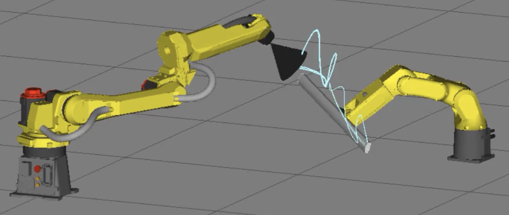
Figure 13: FANUC M10iA (left) + LR Mate 200iD (right) Dual-arm Simulation in RoboGuide for Curve 1.

Curve 1	$max\,\,e_{p}$	$max\,\theta$	$\mu_{avg}$	$\sigma(\mu)/\mu_{avg}$
	mm	deg	mm/s	%
Baseline	0.14	0.10	55.54	4.00
Single Opt	0.48	0.63	327.15	4.81
Dual Opt	0.41	2.86	433.55	4.64

Curve 2	$max\,\,e_{p}$	$max\,\theta$	$\mu_{avg}$	$\sigma(\mu)/\mu_{avg}$
Baseline	0.25	0.34	144.15	4.95
Single Opt	0.39	1.50	679.12	4.95
Dual Opt	0.44	2.26	980.08	1.33

TABLE III: Performance Comparison for FANUC Robots in RoboGuide Simulation

The entire workflow of the motion optimization process is integrated into a Python Qt user interface, as documented in [32], with Tesseract in-browser simulation built in for trajectory visualization.User only needs to provide robot kinematics descriptions in Unified Robotics Description Format (URDF) [33] and the target spatial curve, $(p^{*},n^{*})$, in a Comma-separated values (CSV) file. This interface guides the user through the three steps discussed in Section II and is demonstrated in the supplementary video.

V Conclusion and Future Work

This paper introduces a comprehensive method to generate robot motion program to track complex spatial curves using two industrial robots. The objective is to achieve high and uniform path speed while maintaining specified tracking accuracy. Our approach decomposes the problem into three steps: optimizing robot configuration using continuous robot motion, fitting the robot motion by robot motion primitives, and iteratively updating the waypoints specifying the motion primitives based on the actual tracking error. We demonstrated the efficacy of the approach on ABB robots in simulation and physical experiments, and on FANUC robots in simulation. The experimental setup currently utilizes forward kinematics to calculate the TCP location from the robot joint angles. We are applying the method now to direct measurements of the TCP while the forward kinematics may be imprecise.

References

- [1] H. Chen, T. Fuhlbrigge, and X. Li, “Automated industrial robot path planning for spray painting process: A review,” in 2008 IEEE International Conference on Automation Science and Engineering, 2008, pp. 522–527.
- [2] X. Li, X. Li, S. S. Ge, M. O. Khyam, and C. Luo, “Automatic welding seam tracking and identification,” IEEE Transactions on Industrial Electronics, vol. 64, no. 9, pp. 7261–7271, 2017.
- [3] S. Chen, Z. Wang, A. Chakraborty, M. Klecka, G. Saunders, and J. Wen, “Robotic deep rolling with iterative learning motion and force control,” IEEE Robotics and Automation Letters, vol. 5, no. 4, pp. 5581–5588, 2020.
- [4] K. Ma, X. Wang, and D. Shen, “Design and experiment of robotic belt grinding system with constant grinding force,” in 2018 25th International Conference on Mechatronics and Machine Vision in Practice (M2VIP), 2018, pp. 1–6.
- [5] I. M. Nault, G. D. Ferguson, and A. T. Nardi, “Multi-axis tool path optimization and deposition modeling for cold spray additive manufacturing,” Additive Manufacturing, vol. 38, p. 101779, 2021. [Online]. Available: https://www.sciencedirect.com/science/article/pii/S2214860420311519
- [6] H. He, C.-l. Lu, Y. Wen, G. Saunders, P. Yang, J. Schoonover, J. Wason, A. Julius, and J. T. Wen, “High-speed high-accuracy spatial curve tracking using motion primitives in industrial robots,” in 2023 IEEE International Conference on Robotics and Automation (ICRA), 2023, pp. 12 289–12 295.
- [7] T. Alhart, “Brothers in arms: These robots put a new twist on 3D printing,” 2017. [Online]. Available: https://www.ge.com/news/reports/brothers-arms-robots-put-new-twist-3d-printing
- [8] RoboDK Inc. , Robot Machining with RoboDK.
- [9] Hypertherm, Inc., RobotMaster:CAD/CAM for robots (Off-Line Programming). [Online]. Available: https://www.robotmaster.com,
- [10] OCTOPUZ, RobotMaster:CAD/CAM for robots (Off-Line Programming). [Online]. Available: https://www.octopuz.com/,
- [11] Motoman, Incorporated, Inform II User’s Manual.
- [12] ABB Robotics, Technical reference manual RAPID Instructions, Functions and Data types.
- [13] FANUC Robotics America, Inc., FANUC Robotics SYSTEM R-J3iB Controller KAREL Reference Manual.
- [14] Adept Technology, Inc., V+ Language User’s Guide.
- [15] Staubli Faverges , VAL3 REFERENCE MANUALV+ Language User’s Guide.
- [16] KUKA Roboter GmbH, SOFTWARE KR C1 / KR C2 / KR C3 Reference Guide.
- [17] ABB Robotics, Application manual MultiMove.
- [18] FANUC America Corporation, FANUC America Corporation R-30iB and R-30iB Plus Controller MULTI ARM Controller Option Manual.
- [19] ——, FANUC America Corporation SYSTEM R-30iB and SYSTEM R-30iB Plus Controller Coordinated Motion Setup and Operations Manual.
- [20] YASKAWA MOTOMAN Robotics, DX200 OPTIONSINSTRUCTIONSFOR INDEPENDENT/COORDINATED CONTROL FUNCTION.
- [21] J. Wason, “abb_motion_program_exec,” 2022. [Online]. Available: https://github.com/johnwason/abb_motion_program_exec
- [22] C.-L. Lu, “fanuc_motion_program_exec,” 2022. [Online]. Available: https://github.com/rpiRobotics/fanuc_motion_program_exec
- [23] H. He, “dx200_motion_progam_exec,” 2023. [Online]. Available: https://github.com/rpiRobotics/dx200_motion_progam_exec
- [24] S. Chen, “Robot manipulators intelligent motion and force control,” Ph.D. dissertation, Rensselaer Polytechnic Institute, Troy, NY, 2021.
- [25] ABB Robotics, Product specification IRB 6640.
- [26] ——, Product specification IRB 1200.
- [27] H. He, “Robot_acceleration_identification,” 2023. [Online]. Available: https://github.com/rpiRobotics/Robot_Acceleration_Identification
- [28] R. Storn and K. Price, “Differential evolution – a simple and efficient heuristic for global optimization over continuous spaces,” Journal of Global Optimization, vol. 11, no. 4, pp. 341–359, Dec 1997. [Online]. Available: https://doi.org/10.1023/A:1008202821328
- [29] Y. Wen, H. He, A. Julius, and J. T. Wen, “Motion profile optimization in industrial robots using reinforcement learning,” in 2023 IEEE/ASME International Conference on Advanced Intelligent Mechatronics (AIM), 2023, pp. 1309–1316.
- [30] ABB Robotics, Product manual IRC5.
- [31] ——, Operating Manual RobotStudio.
- [32] rpiRobotics, “Arm-21-02-f-19-robot-motion-program,” 2022. [Online]. Available: https://github.com/rpiRobotics/ARM-21-02-F-19-Robot-Motion-Program
- [33] ROS-Industrial, “Introduction to urdf,” 2017. [Online]. Available: https://industrial-training-master.readthedocs.io/en/melodic/_source/session3/Intro-to-URDF.html