Causal Unit Selection using Tractable Arithmetic Circuits

Abstract

The unit selection problem aims to find objects, called units, that optimize a causal objective function which describes the objects’ behavior in a causal context (e.g., selecting customers who are about to churn but would most likely change their mind if encouraged). While early studies focused mainly on bounding a specific class of counterfactual objective functions using data, more recent work allows one to find optimal units exactly by reducing the causal objective to a classical objective on a meta-model, and then applying a variant of the classical Variable Elimination (VE) algorithm to the meta-model—assuming a fully specified causal model is available. In practice, however, finding optimal units using this approach can be very expensive because the used VE algorithm must be exponential in the constrained treewidth of the meta-model, which is larger and denser than the original model. We address this computational challenge by introducing a new approach for unit selection that is not necessarily limited by the constrained treewidth. This is done through compiling the meta-model into a special class of tractable arithmetic circuits that allows the computation of optimal units in time linear in the circuit size. We finally present empirical results on random causal models that show order-of-magnitude speedups based on the proposed method for solving unit selection.

Introduction

A theory of causality has emerged over the last few decades based on two parallel hierarchies, an information hierarchy and a reasoning hierarchy, often called the causal hierarchy (?; ?). On the reasoning side, this theory has crystallized three levels of reasoning with increased sophistication and proximity to human reasoning: associational, interventional and counterfactual, which are exemplified by the following canonical probabilities. Associational ${\it Pr}(y|x)$: probability of $y$ given that $x$ was observed (e.g., probability that a patient has a flu given they have a fever). Interventional ${\it Pr}(y_{x})$: probability of $y$ given that $x$ was established by an intervention, which is different from ${\it Pr}(y|x)$ (e.g., seeing the barometer fall tells us about the weather but moving the barometer needle won’t bring rain). Counterfactual ${\it Pr}(y_{x}|y^{\prime},x^{\prime})$: probability of $y$ if we were to establish $x$ by an intervention given that neither $x$ nor $y$ are true (e.g., probability that a patient who did not take a vaccine and died would have recovered had they been vaccinated). On the information side, these forms of reasoning require different levels of knowledge, encoded as associational, causal and functional (mechanistic) models, with each class of models containing more information than the preceding one. In the framework of probabilistic graphical models (?), such knowledge is encoded by Bayesian networks (?; ?), causal Bayesian networks (?; ?; ?) and functional Bayesian networks (?) also called structural causal models (SCMs) (?).

The unit selection problem emerged from this theory of causality and has been receiving attention as it provides a rigorous framework to analyze and optimize the causal behavior of objects (e.g., agents). It was initially proposed by (?) who motivated it using the problem of selecting customers to target by an encouragement offer for renewing a subscription. The unit selection problem is based on a causal objective function which mentions a special set of variables ${\bf U}$, called unit variables, and can include any quantities from the causal hierarchy: associational, interventional, or counterfactual. The goal of this problem is to find an instantiation ${\bf u}$ of unit variables which optimizes the given objective function. Intuitively, this is meant to identify units (${\bf u}$), which can be individuals or arbitrary objects such as policies, based on their causal behavior.

Unit selection embeds two subproblems which are hard in general: evaluation and optimization of the objective function (?). Prior work focused on the evaluation problem, which is concerned with estimating the value of a causal objective function using observational and experimental data given a non-parametric causal graph. This stems from the identifiability problem, which has been extensively studied by the causality community. Useful bounds and criteria have been derived for this purpose with respect to a specific causal objective function called the benefit function  (?; ?; ?; ?; ?).

A recent work (?) investigated the optimization problem: finding units that maximize the score defined by the causal objective function—assuming a fully specified SCM so as to obtain point-values for the objective function. They first show that a broad class of causal objective functions can be reduced to an associational probability on a meta-model, called the objective model. They also showed that optimizing this (surrogate) probability requires solving a variant of the Maximum A Posteriori (MAP) inference problem, called Reverse-MAP (R-MAP). They further showed how to modify the classical Variable Elimination (VE) algorithm to solve R-MAP. This treatment, in principle, would allow us to find the exact optimal units. However, computing R-MAP on the objective model remains a hard task—in fact, it is $\text{NP}^{\text{PP}}$-complete as shown in (?). In practice, the objective model is usually much larger and denser than the original SCM. Moreover, running VE on the objective model must be exponential in its constrained treewidth (?), and can also be exponential in the number of unit variables depending on the form of the specific objective function.

We address this computational challenge by introducing a new method for solving R-MAP on a model $G$ by compiling $G$ into a tractable arithmetic circuit (AC) (?; ?) and computing R-MAP on the circuit in linear time. Using ACs for inference allows us to exploit the local/parameteric structure of a model which means that we may be able to handle models that are out of reach of classical, structure-based inference algorithms like VE; see, e.g., (?; ?; ?). And this is indeed what our empirical evaluation shows.

This paper is structured as follows. We start by a review of the unit selection problem and its reduction to R-MAP. We then provide some background on ACs and how they can be used to solve MAP in time linear in the AC size. We follow by our proposed linear-time method for solving R-MAP on ACs, and a corresponding empirical evaluation which shows orders-of-magnitude speedups compared to the state-of-the-art. We finally close with some concluding remarks.

Unit Selection by Reduction to Reverse-MAP

A causal objective function is an expression that involves associational (observational), interventional or counterfactual probabilities. We begin by formulating the selection of customers to target by an advertisement using a specific causal objective function called the benefit function. We next review the reduction from unit selection to Reverse-MAP using an objective model. We finally review the computation of Reverse-MAP using variable elimination.

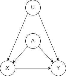
(a) SCM

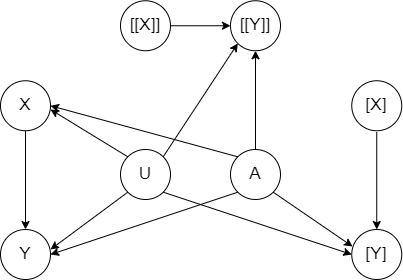
(b) triplet model (mutilated)

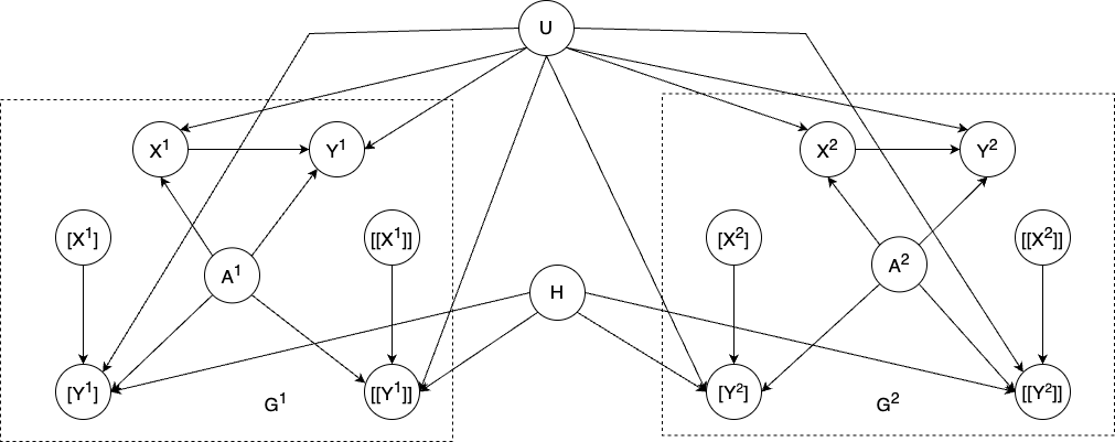
(c) objective model

Figure 1: Example showing the objective model for a causal objective function with 2 components (Huang and Darwiche 2023).

Consider a company that wants to identify customers most likely to respond positively to a pop-up ad of a new product. Suppose the product profit is $50 and the cost of placing the ad to a user is $10. Let variable $Y$ denote whether the user purchases the product (outcome) and variable $X$ denote whether they are targeted by the ad (action). Let variables ${\bf U}$ be the observed customer characteristics (gender, area, purchase history, etc) that affect both $X$ and $Y,$ and variables ${\bf A}$ be the hidden factors that affect $X$ and $Y$. This causal model is shown in Figure 1(a). We can partition customers into four types using counterfactuals. A responder ($y_{x},y_{x^{\prime}}^{\prime}$) purchases the product if targeted but does not otherwise, so the benefit of selecting a responder is $\beta=50-10=40$. An always-taker ($y_{x},y_{x^{\prime}}$) purchases regardless of advertisement, so its benefit is $\gamma=-10$ (the ad cost is lost). An always-denier ($y_{x}^{\prime},y_{x^{\prime}}^{\prime}$) does not purchase regardless of advertisement, so its benefit is $\theta=-10$. A contrarian ($y_{x^{\prime}},y_{x}^{\prime}$) does not purchase if targeted but purchases otherwise, so its benefit is $\delta=-50-10=-60$. The company can then select customers ${\bf u}$ that maximize the benefit function (?; ?; ?):

$$L({\bf u}) =\beta{\it Pr}(y_{x},y_{x^{\prime}}^{\prime}|{\bf u})+\gamma{\it Pr}(y_{x},y_{x^{\prime}}|{\bf u})$$

$$\quad+\theta{\it Pr}(y_{x}^{\prime},y_{x^{\prime}}^{\prime}|{\bf u})+\delta{\it Pr}(y_{x}^{\prime},y_{x^{\prime}}|{\bf u})$$ (1)

This setup was generalized in (?) to (almost) any causal objective function that is a linear combination of counterfactual, interventional, or observational probabilities, which has the following form:

$$L({\bf u})=\sum_{i=1}^{n}w_{i}\cdot{\it Pr}({\bf y}^{i}_{{\bf x}^{i}},{\bf w}^{i}_{{\bf v}^{i}}|{\bf e}^{i},{\bf u})\quad$$ (2)

This class of causal objective functions includes the function in Equation 1 but is more expressive. First, it allows variable sets ${\bf Y}^{i},{\bf W}^{i},{\bf X}^{i},{\bf V}^{i}$ for representing compound treatments and outcomes instead of a single action (ad recommendation) and outcome (purchase). It also allows any combination of their values in each component ${\it Pr}^{i}$. For example, it can include components like ${\it Pr}((\bar{t},b)_{(x,e)},(t,\bar{b})_{(\bar{x},e)}\,|\,{\bf u})$: probability that one would have normal temperature and normal blood pressure $(\bar{t},b)$ had they taken medicine and exercised $(x,e)$, and would have high temperature and low blood pressure $(t,\bar{b})$ had they only exercised $(\bar{x},e)$. Second, it allows evidence ${\bf E}^{i}$ to incorporate what happens in reality. For example, the probability ${\it Pr}(y^{\prime}_{x}\,|\,y,x^{\prime},{\bf u})$ that one would not have gotten Covid $(y^{\prime})$ if they were to be vaccinated $(x)$, given that they did not and contracted Covid $(y,x^{\prime})$. Third, it supports components ${\it Pr}^{i}$ with different treatment and outcome variables, which means that each component of the function can consider different aspects of the problem with different weights. For example, assessing the causal effect of an educational policy that applies $x$ and evaluates students’ SAT score $y$ in the first year; and applies $v$ and evaluates their extracurricular activity $w$ in the second year; e.g., $L({\bf u})=0.7{\it Pr}(y_{x}|{\bf u})+0.3{\it Pr}(w_{v}|{\bf u})$. Finally, we are particularly interested in structured units (e.g., decisions, policies, people, situations, regions, activities) that correspond to many unit variables, so that finding the optimal units poses a scalability problem. We next review the construction of the objective model in (Huang and Darwiche 2023) which reduces this type of objective function to a single observational probability in a principled way.

Objective Model

Consider an SCM $G$ (Figure 1(a)) with unit variables ${\bf U}$. The first step is to reduce each counterfactual component ${\it Pr}({{\bf y}^{i}}_{{\bf x}^{i}},{{\bf w}^{i}}_{{\bf v}^{i}}|{\bf e}^{i},{\bf u})$ to an observational probability on a triplet model $G^{i}$ (see Figure 1(b)). This is done by creating three copies of $G$, denoted by $G$, $[G]$, $[[G]]$ and joining them so that they share all exogenous (root) variables. We then remove edges pointing into treatment variables ${\bf X}^{i}$, ${\bf V}^{i}$ in copies $[G]$ and $[[G]]$ respectively. The counterfactual probability is then reduced to an observational one, ${\it Pr}^{i}([{\bf y}^{i}],[[{\bf w}^{i}]]\,|\,[{\bf x}^{i}],[[{\bf v}^{i}]],{\bf e}^{i},{\bf u}),$ on $G^{i}$. We point out that this is based on a standard technique known as twin-networks (?).

Given a list of triplet models $G^{1},\ldots,G^{n}$, the next step is to combine $(G^{i},{\it Pr}^{i})$ such that the linear combination $\sum{\it Pr}^{i}$ is reduced to a single observational probability. As shown in (?), this can be achieved by adding an auxiliary node $H$ as a common parent of outcome nodes and constraining unit variables ${\bf U}$ among $G^{i}$ to take the same value: if a variable $U\in{\bf U}$ is a root, then it is shared among $G^{i}$; otherwise an auxiliary node is added as a common child for copies of $U$ among $G^{i}$. Node $H$ is called a mixture node as it is responsible for inducing a mixture $\sum{\it Pr}^{i}$. For example, consider an objective function with two components $L(u)=w_{1}\cdot{\it Pr}(y_{x},y^{\prime}_{x^{\prime}}|u)+w_{2}\cdot{\it Pr}(y_{x},y_{x^{\prime}}|u)$. Figure 1(c) shows the corresponding objective model $G^{\prime}$. We can then evaluate $L$ as a classical probability ${\it Pr}^{\prime}([y^{1}],[[{y^{\prime}}^{1}]],[y^{2}],[[y^{2}]]\mid[x^{1}],[[{x^{\prime}}^{1}]],[x^{2}],[[{x^{\prime}}^{2}]],u)$ on $G^{\prime}$. The correctness of the objective model has been studied in-depth (?) and is not the focus of this work. We finally highlight that the problem now amounts to optimizing a classical probability of the form $\max_{{\bf u}}{\it Pr}({\bf e}_{1}|{\bf u},{\bf e}_{2})$ on the objective model, which can be larger and denser than the original SCM.

Reverse-MAP (R-MAP)

Consider an SCM $G$ and let ${\bf U}$, ${\bf E}_{1}$, ${\bf E}_{2}$ be disjoint sets of variables in $G$. The R-MAP problem is defined as $\operatorname{RMAP}({\bf U},{\bf e}_{1},{\bf e}_{2})\triangleq\operatornamewithlimits{argmax}_{{\bf u}}{\it Pr}({\bf e}_{1}|{\bf u},{\bf e}_{2})$ — to be contrasted with the classical MAP problem, $\operatorname{MAP}({\bf U},{\bf e})\triangleq\operatornamewithlimits{argmax}_{\bf u}{\it Pr}({\bf u}|{\bf e})=\operatornamewithlimits{argmax}_{\bf u}{\it Pr}({\bf u},{\bf e})$ (?; ?; ?). In the context of causal reasoning, MAP can be thought of as finding the most likely outcome given a specific cause, while R-MAP is concerned with finding the most likely cause for a specific outcome (given some other information). They are different problems as discussed in (?) and R-MAP captures the essence of unit selection better than MAP.

(?) showed how to adapt the classical variable elimination (VE) algorithm to solve R-MAP. Let ${\bf V}$ be the non-MAP variables. The basic idea is to apply two parallel runs of VE in a synced way. In the first run, we compute ${\it Pr}({\bf U},{\bf e}_{1}{\bf e}_{2})$ by summing out ${\bf V}$ under evidence ${\bf e}_{1}{\bf e}_{2}$. In the second run, we compute ${\it Pr}({\bf U},{\bf e}_{2})$ by summing out ${\bf V}$ under evidence ${\bf e}_{2}$. As shown in (?), we can efficiently “divide” ${\it Pr}({\bf U},{\bf e}_{1}{\bf e}_{2})$ and ${\it Pr}({\bf U},{\bf e}_{2})$ to obtain ${\it Pr}({\bf e}_{1}|{\bf U},{\bf e}_{2})$ if the two runs use the same elimination order. We finally compute the R-MAP probability by maxing out variables ${\bf U}$.

Basics of Arithmetic Circuits

$A$	$B$	$f$
$a$	$b$	$3$
$a$	$\bar{b}$	$4$
$\bar{a}$	$b$	$10$
$\bar{a}$	$\bar{b}$	$12$

Figure 2: An AC that computes factor $f(A,B)$.

An arithmetic circuit (AC) is based on a set of discrete variables, which define a key ingredient of the circuit: the indicators. For each value $x$ of a variable $X$, we have an indicator $\lambda_{x}$. The AC will then have constants (parameters) and indicators (inputs) as its leaf nodes with adders and multipliers as its internal nodes; see Figure 2. An AC represents a factor which is a mapping from variable instantiations to non-negative numbers. A probability distribution is a special case of a factor so an AC can represent a distribution too, which is our focus in this work. The factor represented by an AC is obtained by evaluating the AC at complete variable instantiations. To evaluate the AC at an instantiation ${\bf e}$, we replace each indicator $\lambda_{x}$ with $1$ if the value $x$ is compatible with instantiation ${\bf e}$ and with $0$ otherwise (?). We then evaluate the AC bottom-up in the standard way. The factor $f(A,B)$ in Figure 2 has four rows which correspond to the four instantiations of variables $A$ and $B$. Evaluating the AC in this figure at each of these complete instantiations yields a value for each instantiation and therefore defines its factor. We say in this case that the AC computes this factor. An AC can be evaluated at a partial variable instantiation using the same procedure, but the value returned may not be meaningful unless the circuit satisfies certain properties. Three key such properties are decomposability, determinism and smoothness (?). Let $\operatorname{vars}(n)$ be the subset of variables whose indicators appear at or below a node $n$. Decomposability requires that $\operatorname{vars}(n_{1})\cap\operatorname{vars}(n_{2})=\emptyset$ for every two children $n_{1}$ and $n_{2}$ of a $*$-node. Smoothness requires that $\operatorname{vars}(n_{1})=\operatorname{vars}(n_{2})$ for every two children $n_{1}$ and $n_{2}$ of a $+$-node. Determinism requires at most one non-zero child for each $+$-node, when the circuit is evaluated under any complete variable instantiation. An AC that represents a probability distribution $\Pr({\bf X})$ will return the marginal $\Pr({\bf e})$ when evaluated at input ${\bf e},$ assuming the AC is deterministic, decomposable and smooth (?). It will also compute the MPE probability under evidence ${\bf e}$ in this case, assuming we replace $+$-nodes with $\max$-nodes (?). In fact, determinism is not needed for computing marginals as shown initially in (?) and discussed in detail in (?). See also (?) for a recent tutorial/survey on ACs and their properties.

Solving MAP using Arithmetic Circuits

We next discuss a special class of ACs that we shall utilize in this work: decision-ACs. (?) showed how decision-ACs can be used to solve MAP in time linear in the circuit size, assuming they are constructed subject to specific constraints. (?) built on these observations to show similar results with respect to a problem related to MAP. (?) identified a general condition (determinism after projection) that these constraints ensure, which allows MAP to be solved in linear time. We review these earlier findings next and formalize some of the associated observations as we need them to provide a basis for our treatment for R-MAP.

Definition 1 (Decision-AC).

Let $\mathcal{AC}({\bf X})$ be a decomposable and smooth arithmetic circuit over variables ${\bf X}$. $\mathcal{AC}$ satisfies the decision property if every $+$-node has the form $n=\sum_{i}\lambda_{x_{i}}*n_{i}$ where $x_{i}$ are distinct values of some variable $X\in{\bf X}$ and $n_{i}$ are circuit nodes. We say $X$ is the decision variable of node $n$, denoted $\operatorname{dvar}(n)$.

The decision property implies determinism so decision-ACs are decomposable, smooth and deterministic. Decision-ACs are the numerical analog of the Boolean decision-DNNFs (?) and have been used extensively in probabilistic reasoning (?; ?; ?; ?; ?; ?).

Proposition 1.

Consider a decision-AC over variables ${\bf X}$ and let ${\bf U}\subseteq{\bf X}$. If the circuit satisfies: 1) no $+$-node $n$ with $\operatorname{dvar}(n)\in{\bf U}$ is below some $+$-node $m$ with $\operatorname{dvar}(m)\notin{\bf U}$ and 2) every indicator $\lambda_{x}$ is only attached to some $+$-node $n$ with $\operatorname{dvar}(n)=X$, then this circuit supports linear-time MAP over variables ${\bf U}$.

If a decision-AC satisfies Conditions (1) and (2) above, then we can compute $\operatorname{MAP}({\bf U},{\bf e})$ exactly by traversing the AC bottom-up, while replacing every $+$-node $n$ with decision variable $\operatorname{dvar}(n)\in{\bf U}$ with a $\max$-node. This was first claimed in (?) without a formal proof and was used in later works to solve related problems, e.g., (?; ?). (?) identified Condition (1) of Proposition 1 but Condition (2) was never made explicit in the literature as far as we know but is needed for the proof of Proposition 1. Our proof of this proposition considers a more general condition identified in (?) which allows linear-time MAP on ACs, and then shows that decision-ACs satisfy this condition; see Proposition 2 which is stated later.

Let ${\bf U}$ be the MAP variables and ${\bf V}$ be all other variables. The MAP problem can be solved by first computing the marginal ${\it Pr}({\bf U},{\bf e})=\sum_{\bf V}{\it Pr}({\bf X},{\bf e}),$ which sums-out variables ${\bf V}$ (projects on variables ${\bf U}$), and then computing the MPE, $\max_{\bf U}{\it Pr}({\bf U},{\bf e})$; see, e.g., (?). We know that a decomposable and smooth AC supports linear-time marginals as we can simply set all indicators of variables ${\bf V}$ to $1$. If the AC is also deterministic, then it also supports linear-time MPE. However, after projecting a deterministic, decomposable, and smooth AC on variables ${\bf U},$ the resulting AC over variables ${\bf U}$ may no longer be deterministic. If an AC remains deterministic after being projected on ${\bf U}$, we can easily compute MAP by evaluating the circuit bottom-up while replacing every $+$-node that depends on variables in ${\bf U}$ with a $\max$-node. This was first shown in (?) and the determinism-after-projection property was later referred to as marginal determinism in  (?).

Definition 2.

Consider a decomposable and smooth AC over variables ${\bf X}$ and let ${\bf U}\subseteq{\bf X}$. The AC is ${\bf U}$-deterministic iff the following holds: for any $+$-node $n$, if $n$ depends on ${\bf U}$ (i.e., $\operatorname{vars}(n)\cap{\bf U}\neq\emptyset$), then at most one child of $n$ can be non-zero when the AC is evaluated at any input ${\bf u}$.

If an AC is ${\bf U}$-deterministic, then it can be used to compute the MAP probability $\operatorname{MAP}({\bf U},{\bf e})$ under any evidence ${\bf e}$ by performing a simple, bottom-up traversal as below:

$$\operatorname{val}(n)=\begin{cases}1,&\text{if $n=\lambda_{x}$ \& $x\land{\bf e}$ is consistent}\\ 0,&\text{if $n=\lambda_{x}$ \& $x\land{\bf e}$ is inconsistent}\\ p,&\text{if $n$ is a parameter $p$}\\ \prod_{c\in\text{ch}(n)}\operatorname{val}(c)&\text{if $n$ is a product node}\\ \max_{c\in\text{ch}(n)}\operatorname{val}(c)&\text{if $n$ is a sum node}\\ &\text{and $\operatorname{vars}(n)\cap{\bf U}=\emptyset$}\\ \sum_{c\in\text{ch}(n)}\operatorname{val}(c),&\text{if $n$ is a sum node}\\ &\text{and $\operatorname{vars}(n)\cap{\bf U}\neq\emptyset$}\end{cases}$$

The correctness of this procedure is established as follows. Given decomposability and smoothness, by fixing the indicators of variables ${\bf V}$ to 1, we obtain another decomposable and smooth AC that computes the projection ${\it Pr}({\bf U})=\sum_{\bf V}{\it Pr}({\bf U},{\bf V})$. We can then reduce nodes that do not depend on ${\bf U}$ to constants (parameters). This leads to a projected AC that depends only on ${\bf U}$, $\mathcal{AC}_{p}({\bf U})$. If $\mathcal{AC}({\bf X})$ is ${\bf U}$-deterministic, then $\mathcal{AC}_{p}({\bf U})$ must be deterministic, so it can compute the MPE probability $\max_{\bf U}{\it Pr}({\bf U})$ in linear time after replacing its $+$-nodes with $\max$-nodes.

We now have the following result which immediately implies Proposition 1 and, hence, shows that decision-ACs with appropriate constraints support linear-time MAP.

Proposition 2.

A decision-AC is ${\bf U}$-deterministic if it satisfies the two conditions of Proposition 1.

Proof.

Suppose the decision-AC is evaluated at input ${\bf u}^{*}$ which is some instantiation of ${\bf U}.$ Consider any $+$-node $n$ with decision variable $X$. If $X\in{\bf U}$, it is easy to verify that at most one child of $n$ can be nonzero—the one with indicator $\lambda_{x^{*}}$, where $x^{*}$ is the state of $X$ in ${\bf u}^{*}$. If $X\notin{\bf U}$, we claim that node $n$ cannot depend on ${\bf U}$ (i.e., $\operatorname{vars}(n)\cap{\bf U}=\emptyset$). Hence, this decision-AC is ${\bf U}$-deterministic by Definition 2. We prove this claim by contradiction. Suppose node $n$ does depend on some variable $U\in{\bf U}$, which means there is an indicator $\lambda_{u}$ below $n$. By Condition (2) of Proposition 1, this indicator $\lambda_{u}$ must be attached to some $+$-nodes $m$ with decision variable $U$. This implies that $m$ is below $n$ which contradicts Condition (1) of Proposition 1. ∎

Circuits for Reverse-MAP

We now consider the main question behind our proposed method for unit selection: under what condition, and why, will a circuit attain the ability to support efficient R-MAP? The answer is motivated by the following observation.

Circuit Division

The primitive operation required by R-MAP, beyond the existing ones for classical MAP, is the ability to divide two distributions that have the same domain. That is, to obtain ${\it Pr}({\bf e}_{1}|{\bf U},{\bf e}_{2})$, we need to divide ${\it Pr}({\bf U},{\bf e}_{1}{\bf e}_{2})$ and ${\it Pr}({\bf U},{\bf e}_{2})$ which is generally hard. Hence, we raise the question: given two distributions ${\it Pr}_{1}({\bf X})$ and ${\it Pr}_{2}({\bf X})$ computed using ACs, can we efficiently obtain an AC that computes their quotient ${\it Pr}_{3}({\bf X})={\it Pr}_{1}({\bf X})/{\it Pr}_{2}({\bf X})$? We show that this is feasible if ${\it Pr}_{1}({\bf X})$ and ${\it Pr}_{2}({\bf X})$ are computed by two ACs with the same structure (but with different parametrizations), assuming the ACs are deterministic, decomposable and smooth.

Theorem 1.

Consider an AC that is deterministic, decomposable and smooth under both parametrization $\boldsymbol{\Theta}_{1}$ and $\boldsymbol{\Theta}_{2}$. Suppose further the AC computes distribution ${\it Pr}_{1}({\bf X})$ under $\boldsymbol{\Theta}_{1}$ and distribution ${\it Pr}_{2}({\bf X})$ under $\boldsymbol{\Theta}_{2}$. Then the AC is deterministic, decomposable and smooth and computes ${\it Pr}_{3}({\bf X})={\it Pr}_{1}({\bf X})/{\it Pr}_{2}({\bf X})$ under parametrization $\boldsymbol{\Theta}_{3}=\{\theta_{1}/\theta_{2}:\theta_{1},\theta_{2}\text{ are corresponding parameters in }\boldsymbol{\Theta}_{1},\boldsymbol{\Theta}_{2}\}$.

Hence, we can divide two distributions ${\it Pr}_{1}$ and ${\it Pr}_{2}$ induced by the same AC by simply dividing the corresponding parameters in the ACs that lead to ${\it Pr}_{1}$ and ${\it Pr}_{2}$. Decomposability and smoothness are not enough though, we also need determinism. To prove Theorem 5, we need the notion of a subcircuit which is introduced in (?) and studied extensively in (?).

Definition 3.

Let $\mathcal{AC}({\bf X})$ be a decomposable and smooth circuit. A complete subcircuit $\alpha$ of $\mathcal{AC}$ is obtained by visiting the circuit nodes top-down starting at the root: if a $*$-node is visited, visit all its children, and if $+$-node is visited, visit exactly one of its children. The term of $\alpha$ is the set of variable values appearing in indicators of $\alpha$, and the coefficient of $\alpha$ is the product of all parameters in $\alpha$.

A complete subcircuit must include exactly one indicator for every variable in ${\bf X}$. Hence, the term of each complete subcircuit corresponds to an instantiation ${\bf x}$ of ${\bf X}$, so the subcircuit is called an ${\bf x}$-subcircuit. Evaluating $\mathcal{AC}({\bf x})$ amounts to summing the coefficients of all ${\bf x}$-subcircuits. Furthermore, (?) showed that if the AC is also deterministic, then for any instantiation ${\bf x}$ of ${\bf X}$, if $\mathcal{AC}({\bf x})\neq 0$, there is a unique ${\bf x}$-subcircuit whose coefficient is nonzero. Denote this subcircuit by $\alpha_{\bf x}$. We know $\alpha_{\bf x}$ has coefficient $p_{1}={\it Pr}_{1}({\bf x})$ under $\boldsymbol{\Theta}_{1}$ and coefficient $p_{2}={\it Pr}_{2}({\bf x})$ under $\boldsymbol{\Theta}_{2}$. By construction, $\alpha_{\bf x}$ must have coefficient $p_{3}=p_{1}/p_{2}$ under $\boldsymbol{\Theta}_{3}$. Hence, $\mathcal{AC}({\bf x})=p_{3}={\it Pr}_{3}({\bf x})$ under $\boldsymbol{\Theta}_{3}$. This proves Theorem 5.

Without determinism, an AC may have multiple ${\bf x}$-subcircuits for a given ${\bf x}$, and dividing corresponding parameters may not give the correct result. For a simple example, consider $\mathcal{AC}(X)=a\cdot\lambda_{x}+b\cdot\lambda_{\bar{x}}+c\cdot\lambda_{x}$. $\mathcal{AC}$ is not deterministic; it has two complete subcircuits $(x,a)$ and $(x,c)$ for $x$. We have $\mathcal{AC}(x)=a_{1}+b_{1}$ under $\boldsymbol{\Theta}_{1}$ and $\mathcal{AC}(x)=a_{2}+b_{2}$ under $\boldsymbol{\Theta}_{2}$. After dividing corresponding parameters, $\mathcal{AC}(x)$ produces $a_{1}/a_{2}+b_{1}/b_{2}$ instead of $(a_{1}+b_{1})/(a_{2}+b_{2})$.

SCM			VE				ACE
n	n’	$|{\bf U}|$	done	time (s)	ve_size	tw	done	time (s)	ac_size
10	18.9	3.0	25	0.49	4.92e5	12.28	25	2.09	1595
15	28.4	3.4	25	1.42	9.15e6	16.88	25	3.31	4990
20	36.8	4.0	25	4.72	1.02e8	20.12	25	4.68	1.03e4
25	45.5	5.3	25	45.90	2.42e9	24.16	25	5.76	3.90e4
30	54.5	5.8	22	145.72	8.07e9	27.36	25	13.62	1.12e5
35	63.7	7.0	7	274.73	1.05e10	32.6	24	56.33	3.57e5
40	74.0	10.1	0	/	/	40.0	20	131.78	3.16e6

Table 1: ACE_RMAP v.s. VE_RMAP. Here, $n$ is #nodes we start with to sample SCMs and $n^{\prime}$ is #nodes in the sampled SCM eventually. The “done” column is the number of solved instances out of $25$. Each data point is an average over solved instances.

R-MAP

We now introduce our treatment for solving R-MAP using ACs based on the techniques for MAP and division on ACs. Let ${\bf U}$ be the target variables, ${\bf V}$ be the non-target variables, and ${\bf E}_{1},{\bf E}_{2}$ be evidence variables. Given a ${\bf U}$-deterministic $\mathcal{AC}({\bf X})$ that represents distribution ${\it Pr}({\bf X})$, we can compute the R-MAP probability $\operatorname{RMAP}({\bf U},{\bf e}_{1},{\bf e}_{2})$ by running a two-pass traversal on the AC, similar to how variable elimination is extended to R-MAP.

Let $\mathcal{AC}_{\bf U}$ be the set of nodes in $\mathcal{AC}$ that depend on ${\bf U}$ (i.e., $\operatorname{vars}(n)\cap{\bf U}\neq\emptyset$), and $\mathcal{AC}_{\bf V}$ be the set of nodes that do not (i.e., $\operatorname{vars}(n)\cap{\bf U}=\emptyset$). In the first pass, we evaluate nodes in $\mathcal{AC}_{\bf V}$ bottom-up under input ${\bf e}_{1}{\bf e}_{2}$. This leads to a projected circuit $\mathcal{AC}_{\bf U}({\bf U})$ with parametrization $\boldsymbol{\Theta}_{1}$, which computes ${\it Pr}({\bf U},{\bf e}_{1}{\bf e}_{2})$ and is deterministic. In the second pass, we evaluate $\mathcal{AC}_{\bf V}$ bottom-up under input ${\bf e}_{2}$. This leads to $\mathcal{AC}_{\bf U}({\bf U})$ with parametrization $\boldsymbol{\Theta}_{2}$, which computes ${\it Pr}({\bf U},e_{2})$ and is deterministic. What we need is ${\it Pr}({\bf e}_{1}\,|\,{\bf U},{\bf e}_{2})={\it Pr}({\bf U},{\bf e}_{1}{\bf e}_{2})/{\it Pr}({\bf U},{\bf e}_{2})$. By Theorem 5, this is simply done by dividing corresponding parameters in $\boldsymbol{\Theta}_{1}$ and $\boldsymbol{\Theta}_{2}$. As a result, $\mathcal{AC}_{\bf U}({\bf U})$ with parametrization $\boldsymbol{\Theta}_{3}$ must compute ${\it Pr}({\bf e}_{1}\,|\,{\bf U},{\bf e}_{2})$ and remain deterministic. We finally evaluate $\mathcal{AC}_{\bf U}$ bottom-up while setting all indicates to $1$ and replacing every $+$-node in $\mathcal{AC}_{\bf U}$ with a $\max$-node. The R-MAP probability is returned at the root. We now have the following result which follows from the above discussion.

Theorem 2.

Consider a decomposable and smooth $\mathcal{AC}({\bf X})$ and let ${\bf U}\subseteq{\bf X}$. If $\mathcal{AC}$ is ${\bf U}$-deterministic, then it supports R-MAP with target variables ${\bf U}$ in time linear in the AC size.

Empirical Results

We next apply the AC algorithm for R-MAP to solving unit selection problems on random SCMs, and compare its time and complexity to the VE algorithm for R-MAP — VE_RMAP in (?). Our algorithm, ACE_RMAP, is implemented on top of the ACE system which we use to compile the objective model into a decision-AC, and then evaluate the AC by the two-pass traversal as described in the previous section. The task is to find optimal units for the benefit function shown in Equation 1. We next describe the procedure used to generate problem instances.

Problem Generation

We generate random SCM $G$ according to the method in  (?) and carefully choose unit variables ${\bf U}$, outcome variable $Y$, and action variable $X$ of the benefit function $L$ such that ${\bf U},X,Y$ respect meaningful causal relationships. We first generate a DAG $G_{0}$ with $n$ binary nodes and a maximum number of parents $p$. We then convert $G_{0}$ into SCM $G$ by adding a unique root parent for each internal node in $G_{0}$. The resulting $G$ tends to have many roots, which is meant to mimic the structure of SCMs commonly used for counterfactual reasoning. We randomly choose a leaf as outcome $Y$ and an ancestor (cause) of $Y$ as action $X$. We choose unit variables ${\bf U}$ by randomly picking 50% of the variables satisfying the following constraints: a unit variable $U$ must be a common cause (ancestor) of $X,Y$ and $U$ remains a cause (ancestor) of $Y$ after removing all edges incoming into $X$.

For each problem instance $\langle G,{\bf U},X,Y\rangle$, we construct an objective model $G^{\prime}$ by composing triplet-models $G^{1},\ldots,G^{4},$ one for each component in the benefit function, as discussed earlier; see (?) for more details. We then run ACE_RMAP on $G^{\prime}$ to find the optimal units and compare its results against VE_RMAP implemented in NumPy. The computation for each instance is given 10 minutes to complete. For each problem instance, we report the execution time of ACE_RMAP and VE_RMAP. We also report the size of the circuit generated by ACE (ac_size), and the total size of all factors generated by VE (ve_size), which are two comparable parameters that measure the total number of arithmetic operations required by ACE_RMAP and VE_RMAP, respectively. We also report the approximate constrained treewidth (tw) of $G^{\prime}$, which is computed using minfill heuristics (?) to find a constrained elimination order for VE_RMAP; see (?) for the need of a constrained order.

Results

We used $n\in\{10,15,20,25,30,35,40\}$ and $p=6$ which results in SCM with $n^{\prime}\simeq 2n$ nodes and objective model with $\leq 12n$ nodes. For each $n$, we generate 25 instances and report the average statistics in Table 1. We highlight the patterns from the statistics. First, as $n$ increases, the time and the number operations of VE_RMAP grows exponentially and becomes impractical after $n>30$ (running out of memory). This is predicted as VE_RMAP is purely structure-based and must be exponential in the constrained treewidth (tw). Second, ACE_RMAP is much more efficient than VE_RMAP, leading to orders-of-magnitude speedups as a result of exploiting the high-degree of local (parameteric) structure in the objective model (e.g., 0/1 parameters, context-specific independence, parameter equality). This enables ACE_RMAP to support very large and dense models (with $tw>30$) that are normally out-of-reach if such parametric structure is not exploited.

Conclusion

Our main contribution in this paper is a result which shows how we can solve the Reverse-MAP (R-MAP) problem efficiently using ACs. R-MAP is a variant on the classical MAP problem which arises in causal reasoning, particularly the unit selection problem. We evaluated our AC-based method for solving R-MAP (and the unit selection problem) against the state-of-the-art method based on variable elimination, showing orders-of-magnitude speedups. This is a substantial step forward in making causal reasoning more scalable.

Acknowledgement

This work has been partially supported by ONR grant N000142212501.

References

- [Balke and Pearl 1994] Balke, A., and Pearl, J. 1994. Probabilistic evaluation of counterfactual queries. In AAAI, 230–237. AAAI Press / The MIT Press.
- [Balke and Pearl 1995] Balke, A., and Pearl, J. 1995. Counterfactuals and policy analysis in structural models. In UAI, 11–18. Morgan Kaufmann.
- [Bareinboim et al. 2021] Bareinboim, E.; Correa, J. D.; Ibeling, D.; and Icard, T. F. 2021. On Pearl’s hierarchy and the foundations of causal inference. Technical Report, R-60, Colombia University.
- [Chan and Darwiche 2006] Chan, H., and Darwiche, A. 2006. On the robustness of most probable explanations. In Proceedings of the 22nd Conference in Uncertainty in Artificial Intelligence (UAI).
- [Chavira and Darwiche 2005] Chavira, M., and Darwiche, A. 2005. Compiling bayesian networks with local structure. In Proceedings of the 19th International Joint Conference on Artificial Intelligence (IJCAI), 1306–1312.
- [Chavira and Darwiche 2007] Chavira, M., and Darwiche, A. 2007. Compiling Bayesian networks using variable elimination. In Proceedings of the 20th International Joint Conference on Artificial Intelligence (IJCAI), 2443–2449.
- [Chavira and Darwiche 2008] Chavira, M., and Darwiche, A. 2008. On probabilistic inference by weighted model counting. Artificial Intelligence 172(6–7):772–799.
- [Chavira, Darwiche, and Jaeger 2006] Chavira, M.; Darwiche, A.; and Jaeger, M. 2006. Compiling relational bayesian networks for exact inference. Int. J. Approx. Reasoning 42(1-2):4–20.
- [Choi and Darwiche 2017] Choi, A., and Darwiche, A. 2017. On relaxing determinism in arithmetic circuits. In Proceedings of the Thirty-Fourth International Conference on Machine Learning (ICML), 825–833.
- [Choi, Friedman, and Van den Broeck 2022] Choi, Y.; Friedman, T.; and Van den Broeck, G. 2022. Solving marginal map exactly by probabilistic circuit transformations. In International Conference on Artificial Intelligence and Statistics, 10196–10208. PMLR.
- [Choi, Vergari, and Van den Broeck 2020] Choi, Y.; Vergari, A.; and Van den Broeck, G. 2020. Probabilistic circuits: A unifying framework for tractable probabilistic models. UCLA. URL: http://starai. cs. ucla. edu/papers/ProbCirc20. pdf.
- [Darwiche 2003] Darwiche, A. 2003. A differential approach to inference in Bayesian networks. Journal of the ACM (JACM) 50(3):280–305.
- [Darwiche 2004] Darwiche, A. 2004. New advances in compiling cnf to decomposable negation normal form. In Proc. of ECAI, 328–332. Citeseer.
- [Darwiche 2009] Darwiche, A. 2009. Modeling and Reasoning with Bayesian Networks. Cambridge University Press.
- [Darwiche 2021] Darwiche, A. 2021. Tractable boolean and arithmetic circuits. In Neuro-Symbolic Artificial Intelligence, volume 342 of Frontiers in Artificial Intelligence and Applications. IOS Press. 146–172.
- [Dechter and Rish 2003] Dechter, R., and Rish, I. 2003. Mini-buckets: A general scheme for bounded inference. Journal of the ACM (JACM) 50(2):107–153.
- [Halpern 2000] Halpern, J. Y. 2000. Axiomatizing causal reasoning. Journal of Artificial Intelligence Research 12:317–337.
- [Han, Chen, and Darwiche 2022] Han, Y.; Chen, Y.; and Darwiche, A. 2022. On the complexity of counterfactual reasoning. In A causal view on dynamical systems, NeurIPS 2022 workshop.
- [Huang and Darwiche 2007] Huang, J., and Darwiche, A. 2007. The language of search. Journal of Artificial Intelligence Research 29:191–219.
- [Huang and Darwiche 2023] Huang, H., and Darwiche, A. 2023. An algorithm and complexity results for causal unit selection. In 2nd Conference on Causal Learning and Reasoning.
- [Huang et al. 2006] Huang, J.; Chavira, M.; Darwiche, A.; et al. 2006. Solving map exactly by searching on compiled arithmetic circuits. In AAAI, volume 6, 3–7.
- [Kjærulff 1990] Kjærulff, U. B. 1990. Triangulation of graphs-algorithms giving small total state space.
- [Koller and Friedman 2009] Koller, D., and Friedman, N. 2009. Probabilistic Graphical Models - Principles and Techniques. MIT Press.
- [Li and Pearl 2019] Li, A., and Pearl, J. 2019. Unit selection based on counterfactual logic. In IJCAI, 1793–1799. ijcai.org.
- [Li and Pearl 2022a] Li, A., and Pearl, J. 2022a. Unit selection: Case study and comparison with a/b test heuristic. arXiv preprint arXiv:2210.05030.
- [Li and Pearl 2022b] Li, A., and Pearl, J. 2022b. Unit selection with causal diagram. In AAAI, 5765–5772. AAAI Press.
- [Li and Pearl 2022c] Li, A., and Pearl, J. 2022c. Unit selection with nonbinary treatment and effect. CoRR abs/2208.09569.
- [Li et al. 2022] Li, A.; Jiang, S.; Sun, Y.; and Pearl, J. 2022. Unit selection: Learning benefit function from finite population data. arXiv e-prints arXiv–2210.
- [Park and Darwiche 2004] Park, J. D., and Darwiche, A. 2004. Complexity results and approximation strategies for MAP explanations. J. Artif. Intell. Res. 21:101–133.
- [Pearl and Mackenzie 2018] Pearl, J., and Mackenzie, D. 2018. The Book of Why: The New Science of Cause and Effect. Basic Books.
- [Pearl 1988] Pearl, J. 1988. Probabilistic Reasoning in Intelligent Systems: Networks of Plausible Inference. MK.
- [Pearl 2000] Pearl, J. 2000. Causality. Cambridge University Press.
- [Peters, Janzing, and Schölkopf 2017] Peters, J.; Janzing, D.; and Schölkopf, B. 2017. Elements of Causal Inference: Foundations and Learning Algorithms. MIT Press.
- [Pipatsrisawat and Darwiche 2009] Pipatsrisawat, K., and Darwiche, A. 2009. A new d-dnnf-based bound computation algorithm for functional e-majsat. In Twenty-First International Joint Conference on Artificial Intelligence. Citeseer.
- [Poon and Domingos 2011] Poon, H., and Domingos, P. M. 2011. Sum-product networks: A new deep architecture. In UAI, 337–346.
- [Spirtes, Glymour, and Scheines 2000] Spirtes, P.; Glymour, C.; and Scheines, R. 2000. Causation, Prediction, and Search, Second Edition. Adaptive computation and machine learning. MIT Press.