Efficiently Cooling Quantum Systems with Finite Resources:
Insights from Thermodynamic Geometry

Abstract

Landauer’s universal limit on heat dissipation during information erasure becomes increasingly crucial as computing devices shrink: minimising heat-induced errors demands optimal pure-state preparation. For this, however, Nernst’s third law posits an infinite-resource requirement: either energy, time, or control complexity must diverge. Here, we address the practical challenge of efficiently cooling quantum systems using finite resources. We investigate the ensuing resource trade-offs and present efficient protocols for finite distinct energy gaps in settings pertaining to coherent or incoherent control, corresponding to quantum batteries and heat engines, respectively. Expressing energy bounds through thermodynamic length, our findings illuminate the optimal distribution of energy gaps, detailing the resource limitations of preparing pure states in practical settings.

I Introduction

Arguably, one of the most essential tasks in quantum science is the preparation of pure quantum states — equivalent to cooling quantum systems or erasing information. This is a critical prerequisite for quantum computation, where the output state from a calculation must be erased before it can be reused as an input for the next [1]. Failure to achieve sufficiently pure input states directly contributes to computational errors. Furthermore, the necessity for pure states extends to precise timekeeping [2, 3] and accurate measurements [4]. Without adequate purity, possibly due to limited resources or control, the frequency of gate and measurement errors increases, potentially relegating any anticipated ‘quantum advantage’ to mere theoretical conjecture, as illustrated in Fig. 1.

In this sense, thermodynamics links the degree of control over a system with one’s capacity to perform useful tasks. In particular, Landauer formalised a profound connection between physics and information by establishing that a minimum amount of heat must be dissipated when erasing information encoded in any physical system [5]. This universal limit applies to classical and quantum theory and gains prominence as computing devices are miniaturised, rendering them more susceptible to heat-induced errors. Thus, manipulating information with minimal energetic cost is paramount for developing robust and efficient next-generation devices.

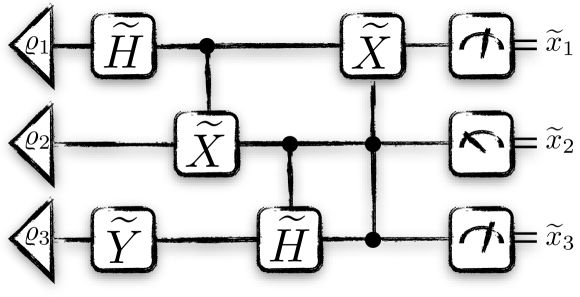
Figure 1: Impact of Imperfect Cooling. A quantum computation begins with a register of $n$ pure states $|{0}\rangle^{\otimes n}$ (not shown), to which gates (e.g., $G\in\{H,X,Y\}$) and measurements are applied, yielding outcomes $\{x_{i}\}_{i=1}^{n}$. Inaccessibility of pure states induces preparation errors leading to noisy initial states $\varrho_{i}\neq|{0}\rangle$, timekeeping errors affecting the gates $G\mapsto\widetilde{G}$, and measurement errors $x_{i}\mapsto\tilde{x}_{i}$.

Efforts to saturate the Landauer bound involve engineering quasistatic interactions between information-carrying systems and controllable machines. However, uncovering the necessary conditions for Landauer-cost erasure has been impeded by inequivalent assumptions and definitions across experimental platforms. A breakthrough by Reeb and Wolf reformulated the Landauer limit universally in the context of quantum information, providing platform-agnostic insights [6]. Their work demonstrated the need for an infinitely large energy gap in an infinite-dimensional machine to achieve perfect Landauer-cost erasure. Such progress notwithstanding, such infinite resources are not practically accessible, leading to the pragmatic problem of optimising cooling with finite resources [7]. When resources are limited, various factors influence the eventual purity of the system and the costs involved, including the energy-level structure of the cooling machines and the complexity of their interactions with the target [8].

Here, we unveil a three-way trade-off among crucial resources — energy, time, and control complexity. We explore this relationship in the regime where finite resources dictate the attainable temperature and cooling rate. Our investigation leverages the geometric technique of thermodynamic length [9, 10, 11, 12] to yield insights into the optimal energy structure of cooling machines for schemes using fixed control complexity and large yet finite time, thus contributing to the understanding of resource limitations in preparing pure states.

II Thermodynamic Framework

Setting.—We consider the task of cooling a target quantum system $S$ via unitary interactions with another system $M$, composed of $N$ subsystems $\{M_{1},\ldots,M_{N}\}$ called machines. We describe the overall cooling procedure using a Markovian collision model [13, 14, 15, 16, 17, 18]. Here, the target unitarily interacts with a fresh machine at each time, reflecting the property of memorylessness and the rapid rethermalisation of machines between control operations (see Fig. 2).

All systems $X\!\in\!\{S,M_{1},\ldots,M_{N}\}$ have an associated Hilbert space $\mathcal{H}_{\raisebox{0.0pt}{\tiny{$X$}}}$, on which states $\varrho_{\raisebox{0.0pt}{\tiny{$X$}}}$ are represented as positive semidefinite, unit-trace operators. Each system has a Hamiltonian whose spectral decomposition fixes its energy structure, $H_{\raisebox{0.0pt}{\tiny{$X$}}}\!:=\!\sum_{i=0}^{d_{\raisebox{0.0pt}{\tiny{$X$}}}-1}E_{\raisebox{0.0pt}{\tiny{$X$}}}^{\hskip 1.0pt\raisebox{0.0pt}{\tiny{$(i)$}}}|{i}\rangle\!\langle{i}|$. We consider finite-dimensional systems $d_{\raisebox{0.0pt}{\tiny{$X$}}}\!:=\!\mathrm{dim}(\mathcal{H}_{\raisebox{0.0pt}{\tiny{$X$}}})\!<\!\infty$, and assume that energy eigenvalues are ordered non-decreasingly $E_{\raisebox{0.0pt}{\tiny{$X$}}}^{\hskip 1.0pt\raisebox{0.0pt}{\tiny{$(i\!+\!1)$}}}\!\geq\!E_{\raisebox{0.0pt}{\tiny{$X$}}}^{\hskip 1.0pt\raisebox{0.0pt}{\tiny{$(i)$}}}$, with $E_{\raisebox{0.0pt}{\tiny{$X$}}}^{\hskip 1.0pt\raisebox{0.0pt}{\tiny{$(0)$}}}:=0$. With respect to any Hamiltonian $H$, the thermal (Gibbs) state at inverse temperature $\beta:=(k_{\raisebox{0.0pt}{\tiny{$\mathrm{B}$}}}T)^{-1}$ is $\tau(\beta,H):=\mathcal{Z}^{-1}(\beta)\exp{(-\beta H)}$, where $\mathcal{Z}(\beta):=\mbox{tr}\left[{\exp{(-\beta H)}}\right]$ is the partition function; when unambiguous, we will simply write $\tau(\beta)$. The thermal state uniquely maximises entropy $S(\varrho):=-\mbox{tr}\left[{\varrho\log{\varrho}\hskip 0.5pt}\right]$ for fixed average energy $\hbox to0.0pt{\hskip 1.47914pt\leavevmode\hbox{\set@color$\overline{\hbox{}}$}\hss}{\leavevmode\hbox{\set@color$E$}}(\varrho):=\mbox{tr}\left[{H\varrho\hskip 0.5pt}\right]$. Consequently, it provides a state description with minimal information (beyond average energy), and is thus a suitable initial machine state for cooling schemes (formalised below).

Boundary Conditions.—We consider procedures that take the target system from an initial state $\varrho_{\raisebox{0.0pt}{\tiny{$S$}}}$ to a final one $\varrho^{\prime}_{\raisebox{0.0pt}{\tiny{$S$}}}$, whilst mapping the collection of machines from an initial thermal state $\tau_{\raisebox{0.0pt}{\tiny{$M$}}}(\beta)$ to a final state $\varrho_{\raisebox{0.0pt}{\tiny{$M$}}}^{\prime}$, via the global evolution

$$\varrho^{\prime}_{\raisebox{0.0pt}{\tiny{$SM$}}}=U(\varrho_{\raisebox{0.0pt}{\tiny{$S$}}}\otimes\tau_{\raisebox{0.0pt}{\tiny{$M$}}}(\beta))U^{\dagger}.$$ (1)

Note that cooling a system can have several inequivalent meanings. For equilibrium processes, it could mean reducing the temperature of a thermal state; in non-equilibrium settings, it could mean increasing the ground-state population or purity of the target, or decreasing its entropy or average energy. The strongest notion of cooling derives from the preorder on states induced by majorisation: We say that a state $\varrho$ is colder than $\sigma$ iff $\varrho\succ\sigma$. Since all meaningful notions of temperature are Schur-convex/concave functions of the vector of non-decreasing energy eigenvalues, any other such quantifier would agree that $\varrho$ is colder than $\sigma$ [19]. Although all qualitative results presented here hold true in this strong sense, for the sake of simplicity, we focus on processes that take the target system from a Gibbs state with some initial $\beta$ to one with final value $\beta_{\mathrm{f}}:=\lambda\beta$ with $\lambda>1$.

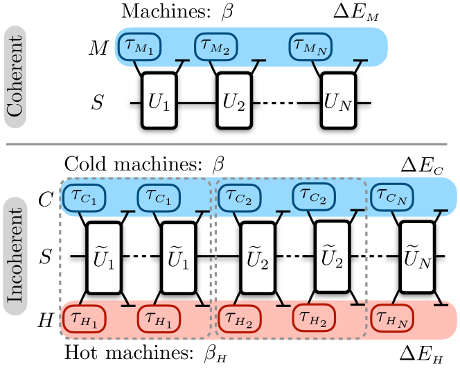
Figure 2: Framework. A system $S$ is cooled via sequential interactions with a system $M$ comprising $N$ machines. The interaction is described by a collision model that is ensured to be Markovian by discarding used machines between steps. In the coherent-control setting (top panel), arbitrary unitaries $U_{i}$ can be implemented between $S$ and the machines, which are each initially in thermal states $\tau_{\raisebox{0.0pt}{\tiny{$M_{i}$}}}(\beta,H_{\raisebox{0.0pt}{\tiny{$M_{i}$}}})$. In the incoherent-control setting (bottom panel), the cooling system $M$ is split into a hot $(H)$ and cold ($C$) system, at inverse temperatures $\beta_{\raisebox{0.0pt}{\tiny{$H$}}}$ and $\beta$, respectively. Again, each machine is endowed with its own Hamiltonian $H_{\raisebox{0.0pt}{\tiny{$X_{i}$}}}$ for $X\in\{C,H\}$; in the incoherent-control setting, the unitaries are restricted to be energy conserving, i.e., $[\widetilde{U}_{i},H_{\raisebox{0.0pt}{\tiny{$S$}}}+H_{\raisebox{0.0pt}{\tiny{$C_{i}$}}}+H_{\raisebox{0.0pt}{\tiny{$H_{i}$}}}]=0$. Moreover, we allow repeated interactions between the target and copies of each hot and cold machine, which we refer to as a stage (grey dashed outline). In both settings, the energy cost is associated to the change in energy of the appropriate cooling system, i.e., $\Delta E_{\raisebox{0.0pt}{\tiny{$X$}}}$ for $X\in\{M,C,H\}$.

Structural and Control Resources.—Various factors determine a protocol’s performance, including the dimensions $d_{\raisebox{0.0pt}{\tiny{$X$}}}$ and Hamiltonians $H_{\raisebox{0.0pt}{\tiny{$X$}}}$ of all systems, the interaction range $k$ (denoting the number of systems involved in each interaction), the number of machines $N$, and the dissipated heat $\Delta E_{\raisebox{0.0pt}{\tiny{$M$}}}:=\mbox{tr}\left[{H_{\raisebox{0.0pt}{\tiny{$M$}}}(\varrho_{\raisebox{0.0pt}{\tiny{$M$}}}^{\prime}-\varrho_{\raisebox{0.0pt}{\tiny{$M$}}})}\right]$, which sets a lower bound for the energetic cost of any implementation. We distinguish between structural resources, such as $d_{\raisebox{0.0pt}{\tiny{$X$}}}$ and $H_{\raisebox{0.0pt}{\tiny{$X$}}}$, that are fixed independently of the procedure, and control resources linked to the protocol’s execution, such as the interaction range $k$, total duration (represented by $N$ for fixed $k$), and the dissipated heat $\Delta E_{\raisebox{0.0pt}{\tiny{$M$}}}$.

Type of Control.—We consider two extremal control paradigms: coherent and incoherent. Coherent control permits drawing upon a work source to implement any system-machine unitary. In contrast, incoherent control relies upon energy-conserving unitaries between the target system and machines at different temperatures [20, 21, 8]. The former corresponds to the highest level of control in a thermodynamic setting, whereas the latter assumes less control, only requiring interaction Hamiltonians to be switched on and off to induce transitions. The settings of heat-bath algorithmic cooling [22, 23, 24, 25, 26, 27, 28] and of autonomous cooling [29, 30, 31, 32, 33, 34, 35] are contained within the coherent and incoherent control paradigms, respectively.

Cooling Schemes.—We now define the concept of a cooling scheme, encompassing all aforementioned dependencies.

Definition 1.

A cooling scheme is defined by the tuple: $(\mathscr{B},\mathscr{S},\mathscr{C},\mathscr{T})$. Here, $\mathscr{B}$ denotes the boundary conditions of the problem, namely, the initial and final temperature of the target system. The structural resources $\mathscr{S}$ comprise $\beta$, $H_{\raisebox{0.0pt}{\tiny{$X$}}}$, and $d_{\raisebox{0.0pt}{\tiny{$X$}}}$, i.e., the initial temperature, Hamiltonians, and dimensions of all systems. The control resources $\mathscr{C}$ encompass the total number $N$ of machines, the interaction range $k$, and the energy cost $\Delta E_{\raisebox{0.0pt}{\tiny{$M$}}}$. Finally, the type $\mathscr{T}$ indicates whether the procedure operates within the coherent or incoherent setting.

Two remarks are in order. First, not all tuples correspond to physically implementable cooling schemes, given that for either type $\mathscr{T}$ certain combinations of structural $\mathscr{S}$ and/or control resources $\mathscr{C}$ may render certain boundary conditions $\mathscr{B}$ unattainable. Notably, Nernst’s third law of thermodynamics and Landauer’s bound exemplify instances where particular resource configurations preclude specific boundary conditions. Concretely, Nernst’s law states that infinite resources are required to prepare a pure state [36, 37, 38]; in our context, an infinitely large energy gap in the machine is necessary [6, 20, 8]. Similarly, Landauer’s bound establishes that the entropy of the target system cannot be reduced by $\widetilde{\Delta}S:=S(\varrho_{\raisebox{0.0pt}{\tiny{$S$}}})-S(\varrho_{\raisebox{0.0pt}{\tiny{$S$}}}^{\prime})$ via interactions with a thermal machine without incurring an energetic cost of at least $\beta\Delta E_{\raisebox{0.0pt}{\tiny{$M$}}}$ [5, 1, 39, 6]. Delineating the boundary of achievable cooling procedures for different resource configurations represents a significant open problem [8, 7]. Here, we focus on achievable schemes, optimising over specific resources to attain effective cooling procedures. Second, a cooling scheme does not correspond to a unique sequence of applied operations: Different control sequences may yield identical thermodynamic behaviour. We focus on protocols that impact the thermodynamics, neglecting coherences and correlations potentially introduced by certain operations to ensure maximal resource efficiency [40, 41, 42].

III Thermodynamic geometry

We now analyse the impact of structural resources for fixed control complexity in the finite-resource regime. Here structural complexity is determined by the energy-level structure of machines and control complexity quantifies the number of involved systems in each collision. As demonstrated in Ref. [8], infinite resources permit perfect cooling of the target system to its ground state with Landauer’s energy cost; in particular, a machine of infinite structural complexity, i.e., with a diverging number of distinct energy gaps, is necessary. Given our restriction to finite resources, we aim to bound the cooling effectiveness and energy costs for Markovian collision models.

We seek the optimal energy-level structure of machines and interactions to minimise the energy cost of a cooling scheme characterised by fixed control complexity and finite duration. Specifically, we assume the ability to implement $N$ unitary interactions, each of fixed complexity, between the target system and fresh machines. Recall that the objective is to take the target from an initial state $\tau_{\raisebox{0.0pt}{\tiny{$S$}}}(\beta,H)$ to a state $\tau_{\raisebox{0.0pt}{\tiny{$S$}}}(\beta_{\mathrm{f}}:=\lambda\beta,H)$ with lower temperature, i.e., $\lambda>1$. By fixed complexity, we refer to the use of (finitely many) $k$-partite unitaries involving the target and $k-1$ fresh machines in each step (for finite $k$). We quantify the duration of the protocol via the number of operation steps $N$. Our first goal is to identify the optimal set of machine Hamiltonians $\{H_{M_{i}}\}_{i}$ that minimises the dissipated heat throughout the protocol. To achieve this objective, we leverage the concept of thermodynamic length [11, 43, 9, 44].

To this end, consider a path in Hamiltonian space $H(t)$ parameterised by $t\in[0,1]$. The thermodynamic length associated to such a path is given by

$$\mathcal{L}:=\int_{0}^{1}\sqrt{\mathrm{cov}_{t}\bigl{(}\dot{H}(t),\dot{H}(t)\bigr{)}}\,\text{d}t.$$ (2)

where $\dot{H}(t):=\partial_{t}H(t)$ and

$$\text{cov}_{t}(A,B):=\mbox{tr}\left[{\mathcal{J}_{t}(A)B}\right]-\mbox{tr}\left[{\varrho A}\right]\mbox{tr}\left[{\varrho B}\right],$$ (3)

with $\mathcal{J}_{t}(A):=\int_{0}^{1}\tau(\beta,H(t))^{1-x}A\tau(\beta,H(t))^{x}\,\textup{d}x$. The length squared $\mathcal{L}^{2}$ is related to the dissipated heat or excess work when slowly driving $H(t)$ whilst in contact with a bath at inverse temperature $\beta$ [10, 11, 12]. The minimal length connecting two endpoints then corresponds to the minimal dissipation along a path in the Hamiltonian space and is found by the solving the geodesic equations; for the form (2), an analytic solution is known [45].

We aim to exploit the framework of thermodynamic geometry, typically employed in slowly driven systems  [46, 47, 48, 49, 50], to bring new insights to our question of interest: Given the ability to apply $N$ unitary interactions (of fixed complexity $k$) between system and machines, what is the optimal energy-level distribution of the machines for cooling the target system?

IV Coherent control

In the coherent-control setting, given infinite resources, the Landauer bound sets the ultimate limit on cooling. Our first focus is to examine the role of finite structural complexity in said scenarios. Specifically, we strive to identify the structural complexity that minimises the energy cost when the system is cooled via a sequence of $N\!<\!\infty$ bipartite ($k\!=\!2$) interactions.

Theorem 1.

In the coherent-control setting, given a qudit system with Hamiltonian $H$, the minimum energy cost of cooling from a thermal state $\tau_{\raisebox{0.0pt}{\tiny{$S$}}}(\beta,\,H)$ to $\tau_{\raisebox{0.0pt}{\tiny{$S$}}}(\lambda\beta,H)$ using swaps between the system and a fresh qudit machine with arbitrary Hamiltonian at each of the $N$ steps, is given by

$$\beta\Delta E_{\raisebox{0.0pt}{\tiny{$M$}}}=\widetilde{\Delta}S_{\raisebox{0.0pt}{\tiny{$S$}}}+\frac{\beta^{2}}{2N}(\mathcal{L}^{*})^{2}+\mathcal{O}(N^{-2}),$$ (4)

where $\mathcal{L}^{*}$ is the minimal thermodynamic length [45, 44]:

$$\mathcal{L}^{*} =2\arccos\left(\mathrm{tr}\left[\sqrt{\tau_{\raisebox{0.0pt}{\tiny{$S$}}}(\beta,\,H)}\sqrt{\tau_{\raisebox{0.0pt}{\tiny{$S$}}}(\lambda\beta,H)}\right]\right)$$

$$=2\arccos\left(\frac{\mathcal{Z}(\beta(1+\lambda)/2)}{\sqrt{\mathcal{Z}(\beta)\mathcal{Z}(\lambda\beta)}}\right).$$ (5)

Sketch of proof. The proof, fully detailed in Appendix A, is based on the equality form of Landauer’s bound [6]:

$$\beta\Delta E_{\raisebox{0.0pt}{\tiny{$M$}}}=\widetilde{\Delta}S_{\raisebox{0.0pt}{\tiny{$S$}}}+I(S\!:\!M)_{\varrho_{\raisebox{0.0pt}{\tiny{$SM$}}}^{\prime}}+D(\varrho_{\raisebox{0.0pt}{\tiny{$M$}}}^{\prime}\hskip 0.5pt\|\hskip 0.5pt\tau_{\raisebox{0.0pt}{\tiny{$M$}}}(\beta)),$$ (6)

which holds for any transformation described by Eq. (1) such that the entropy of the target changes from $S(\varrho_{\raisebox{0.0pt}{\tiny{$S$}}})$ to $S(\varrho_{\raisebox{0.0pt}{\tiny{$S$}}}^{\prime})=S(\varrho_{\raisebox{0.0pt}{\tiny{$S$}}})-\widetilde{\Delta}S_{\raisebox{0.0pt}{\tiny{$S$}}}$. Here, $I(X\!:\!Y)_{\varrho_{\raisebox{0.0pt}{\tiny{$XY$}}}}:=S(\varrho_{\raisebox{0.0pt}{\tiny{$X$}}})+S(\varrho_{\raisebox{0.0pt}{\tiny{$Y$}}})-S(\varrho_{\raisebox{0.0pt}{\tiny{$XY$}}})$ is the quantum mutual information and $D(\varrho_{\raisebox{0.0pt}{\tiny{$X$}}}\hskip 0.5pt\|\hskip 0.5pt\varrho_{\raisebox{0.0pt}{\tiny{$Y$}}}\!):=\mbox{tr}\left[{\varrho_{\raisebox{0.0pt}{\tiny{$X$}}}(\log{\varrho_{\raisebox{0.0pt}{\tiny{$X$}}}}-\log{\varrho_{\raisebox{0.0pt}{\tiny{$Y$}}}}\!)}\right]$ is the quantum relative entropy. The proof then proceeds in two steps: First, the bipartite interactions are chosen to be swaps between the qudit system and each of a sequence of qudit machines with increasing energy gaps, such that no correlations are built up between $S$ and $M$ as the system is cooled, i.e., $I(S\!:\!M)_{\varrho_{SM}^{\prime}}=0$. Then, the relative-entropy term is minimised; for the sequence of swap operations considered, the relative entropy has the tight lower bound $\tfrac{\beta^{2}}{2N}(\mathcal{L}^{*})^{2}+\mathcal{O}(N^{-2})$, and we thus assert the claim. ∎

To summarise, having fixed the parameters $d_{\raisebox{0.0pt}{\tiny{$X$}}}<\infty$, $N<\infty$, and $k=2$, but not the structural complexity, i.e., the machine Hamiltonians $\{H_{\raisebox{0.0pt}{\tiny{$M_{i}$}}}\}_{i}$, of a coherent-control cooling scheme, we have optimised the remaining control-resource parameter, namely the energy cost $\Delta E_{\raisebox{0.0pt}{\tiny{$M$}}}$. In the case of qubit target and machines, we show that such swaps indeed constitute the optimal interaction (see Appendix A.1) and derive the Hamiltonian that saturates Eq. (4) (see Appendix A.2), thereby providing the optimal cooling scheme with respect to heat dissipation in the case of qubits. In Fig. 3, we compare this optimal protocol with other known coherent cooling schemes to demonstrate its effectiveness. Although the optimal energy structure in the case of swaps for higher dimensions is given by Eq. (1), determining the optimal operation in general remains an open problem.

Moreover, two comments regarding optimality are in order. First, we are assuming that the cooling procedure is Markovian, i.e., that the machines are completely refreshed between steps of controlled evolution. In this setting, creating correlations costs energy [40, 41, 42], which implies that the optimal scheme should minimise the correlations built up between system and machines [51, 52]. However, in a non-Markovian setting, correlations could potentially be used in later steps to lower the energy cost or improve performance [53, 54, 18]. Second, there is a non-zero energy cost for creating coherences [55]. Since we assume an initial state that is diagonal in the energy eigenbasis, this implies that the optimal cooling scheme must only permute populations of energy eigenstates, but for general initial states this need not be the case.

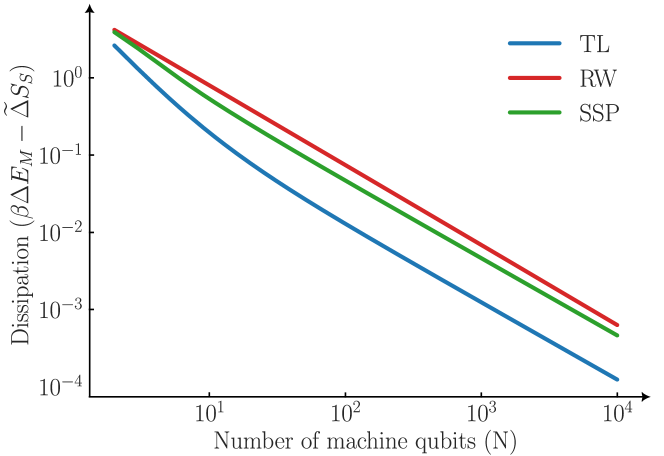
Figure 3: Cooling with Coherent Control. Here we plot the dissipation when coherently cooling a qubit target with energy gap $E_{S}=1$ from $\beta=10^{-8}$ to $\beta_{\mathrm{f}}=10$ (i.e., $\lambda=10^{9}$) via a sequence of bipartite interactions with $N$ machine qubits. We compare three different cooling procedures that depend on the energy-level structure $\{H_{M_{i}}\}_{i}$: TL corresponds to the optimal protocol deduced from the thermodynamic length (see Theorem 1); RW corresponds to the protocol from Ref. [6] where machine energy gaps change linearly; SSP corresponds to the protocol from Ref. [56] where the machine qubits’ excited state populations change linearly.

V Incoherent control

We now consider the same question within the incoherent-control setting. In contrast to the coherent-control setting, all heat and entropy flows now occur solely by coupling the target system to a hot ($H$) and cold ($C$) machine, leading to an energy-conserving transformation overall. Beginning with $\varrho_{\raisebox{0.0pt}{\tiny{$SC{}H$}}}=\tau_{\raisebox{0.0pt}{\tiny{$S$}}}(\beta)\otimes\tau_{\raisebox{0.0pt}{\tiny{$C$}}}(\beta)\otimes\tau_{\raisebox{0.0pt}{\tiny{$H$}}}(\beta_{\raisebox{0.0pt}{\tiny{$H$}}})$, where $\beta_{\raisebox{0.0pt}{\tiny{$H$}}}<\beta$, the considered evolution leads to the output state $\varrho_{\raisebox{0.0pt}{\tiny{$SC{}H$}}}^{\prime}=\widetilde{U}\varrho_{\raisebox{0.0pt}{\tiny{$SC{}H$}}}\widetilde{U}^{\dagger}$, where $[\widetilde{U},H_{\raisebox{0.0pt}{\tiny{$S$}}}+H_{\raisebox{0.0pt}{\tiny{$C$}}}+H_{\raisebox{0.0pt}{\tiny{$H$}}}]=0$ encodes energy conservation.

In this setting, the Landauer bound is unattainable; instead, the ultimate limit is given by the Carnot-Landauer bound [8]

$$\Delta F_{\raisebox{0.0pt}{\tiny{$S$}}}^{\beta}+\eta\Delta E_{\raisebox{0.0pt}{\tiny{$H$}}} \leq 0,$$ (7)

which follows from the equality form

$$\Delta F_{\raisebox{0.0pt}{\tiny{$S$}}}^{\beta}+\eta\,\Delta E_{\raisebox{0.0pt}{\tiny{$H$}}} =\,-\beta^{-1}[\Delta S_{\raisebox{0.0pt}{\tiny{$S$}}}\,+\,\Delta S_{\raisebox{0.0pt}{\tiny{$C$}}}\,+\,\Delta S_{\raisebox{0.0pt}{\tiny{$H$}}}\,$$ (8)

$$\ \ +\,D(\varrho_{\raisebox{0.0pt}{\tiny{$C$}}}^{\prime}\hskip 0.5pt\|\hskip 0.5pt\tau_{\raisebox{0.0pt}{\tiny{$C$}}}(\beta))\,+\,D(\varrho_{\raisebox{0.0pt}{\tiny{$H$}}}^{\prime}\hskip 0.5pt\|\hskip 0.5pt\tau_{\raisebox{0.0pt}{\tiny{$H$}}}(\beta_{\raisebox{0.0pt}{\tiny{$H$}}}))].$$

Here, we have introduced the free energy $F_{\raisebox{0.0pt}{\tiny{$X$}}}^{\beta}(\varrho):=\mbox{tr}\left[{H_{\raisebox{0.0pt}{\tiny{$X$}}}\varrho\hskip 0.5pt}\right]-\beta^{-1}S(\varrho)$ and the Carnot efficiency $\eta:=1-\beta_{\raisebox{0.0pt}{\tiny{$H$}}}/\beta\in[0,1]$.

In a similar vein to the coherent-control scenario, we wish to bound the right-hand side of Eq. (8) for any finite-resource implementation, and ideally identify a protocol that saturates this bound. However, a number of problems immediately arise in the incoherent-control scenario, since one is restricted to the orbit of energy-conserving unitaries, i.e., $\widetilde{U}$ such that $[\widetilde{U},H_{\raisebox{0.0pt}{\tiny{$S$}}}+H_{\raisebox{0.0pt}{\tiny{$C$}}}+H_{\raisebox{0.0pt}{\tiny{$H$}}}]=0$. This constraint implies that the relative-entropy terms cannot be bounded simply by the thermodynamic length, which was possible in the coherent-control setting because the full swap led to a straightforward expression in terms of a sequence of relative-entropy terms applied to the chain of machines. Here, such a swap is prohibited by energy conservation. We now present an attainable energy bound for finite-resource cooling with incoherent control, which is generally optimal for qubits, and optimal for qudits within the considered class of interactions, in analogy to Theorem 1 in the coherent-control setting.

Theorem 2.

In the incoherent-control setting, given a qudit system with Hamiltonian $H$, the minimum energy cost for cooling from a thermal state $\tau_{\raisebox{0.0pt}{\tiny{$S$}}}(\beta,\,H)$ to $\tau_{\raisebox{0.0pt}{\tiny{$S$}}}(\lambda\beta,H)$, by using particular tripartite (energy-conserving) interactions between the system and two fresh qudit machines at inverse temperature $\beta$ (cold) and $\beta_{\raisebox{0.0pt}{\tiny{$H$}}}\leq\beta$ (hot), respectively, with arbitrary Hamiltonians in the limit of infinite steps but with $N$$<\infty$ distinct energy gaps, is given by

$$\Delta F_{\raisebox{0.0pt}{\tiny{$S$}}}^{\beta}\,+\eta\,\Delta E_{\raisebox{0.0pt}{\tiny{$H$}}}=\,-\frac{\beta}{2N}(\mathcal{L}^{*})^{2}+\mathcal{O}(N^{-2}).$$ (9)

Sketch of proof. The proof, presented in Appendix B, is fundamentally different to its coherent-control counterpart. In the constructive direction, we propose a cooling scheme comprising interactions that exchange populations amongst levels $|{i,i+1,i}\rangle_{\raisebox{0.0pt}{\tiny{$SCH$}}}\leftrightarrow|{i+1,i,i+1}\rangle_{\raisebox{0.0pt}{\tiny{$SCH$}}}$. The energy-conserving nature allows us to calculate the energy cost per population transfer, which is related to the relative entropy between the initial and final states of the virtual-qubit subspaces of the hot-and-cold machine that permit cooling. We finally bound this quantity by the thermodynamic length. ∎

For qudits, it is not clear that the form of energy-conserving interactions considered here are optimal; nonetheless, within this family, we present a cooling scheme that attains the energy cost of Eq. (9) and saturates the Carnot-Landauer bound in the limit of infinitely many distinct energy gaps, i.e., diverging control complexity. In the special case of cooling a qubit target with (hot and cold) qubit machines, we show that the 3-cycle $|{010}\rangle_{\raisebox{0.0pt}{\tiny{$SC{}H$}}}\leftrightarrow|{101}\rangle_{\raisebox{0.0pt}{\tiny{$SC{}H$}}}$ is indeed optimal. This is because for any fixed set of energy gaps, the family of energy-conserving unitaries on three qubits that permit cooling without creating coherences or correlations must be of this form, and thus we can cover the entire orbit of unitaries in question. Such operations can be considered as a virtual swap between the target and the virtual qubit subspace of the machine spanned by $\{|{01}\rangle_{\raisebox{0.0pt}{\tiny{$CH$}}},|{10}\rangle_{\raisebox{0.0pt}{\tiny{$CH$}}}\}$. In general, since such a subspace has norm strictly less than one, each such virtual swap will lead to the system qubit being at strictly higher temperature than the virtual qubit. However, in the limit of infinitely many repetitions, the temperature of the system’s qubit subspace of interest converges to the virtual temperature of the machine-qubit subspace [20, 21]. As we are interested in finite resources, we assume that one performs a finite but sufficiently large number of virtual swaps so that the error is within specified tolerances. The relative entropy term that governs the finite-cooling behaviour here (and which leads to the thermodynamic-length term) concerns the initial and final thermal states of the machine at the corresponding virtual temperature defined by the qubit subspace in question. Implementing the protocol that swaps the target successively with appropriately chosen virtual qubits of the machine in each stage minimises the thermodynamic length and therefore provides the optimal incoherent cooling procedure.

VI The role of correlations in the incoherent cooling setting

The constraint of energy conservation fundamentally distinguishes the paradigms of coherent and incoherent control. In the latter setting, the virtual subspaces spanned by the hot-and-cold machines significantly influence the performance of a cooling scheme, rather than the state of the machine per se. This suggests that correlations play a dominant role in the incoherent-control setting; we now formalise this intuition.

Theorem 3.

For any incoherent-control cooling scheme, the sum of free energy differences $\Delta F_{\raisebox{0.0pt}{\tiny{$X$}}}^{\beta}$ (with respect to the inverse temperature $\beta$) is bounded by the sum of generated correlations $\Delta I_{\alpha}$,

$$\sum_{\raisebox{0.0pt}{\tiny{$X\!\in\!\{\!S\!,\!C\!,\!H\!\}$}}}\Delta F_{\raisebox{0.0pt}{\tiny{$X$}}}^{\beta}\leq-\tfrac{2}{3}\beta^{-1}\sum_{\alpha}\Delta I_{\alpha},$$ (10)

where $\alpha\in\{SC,SH,CH\}$, and $I_{\raisebox{0.0pt}{\tiny{$XY$}}}:=I(X\!:\!Y)_{\varrho_{\raisebox{0.0pt}{\tiny{$XY$}}}}$ is the quantum mutual information.

A proof is given in Appendix C. This bound has interesting implications. For instance, a priori, in the incoherent control setting, the only claim that one can deduce regarding the free energy change of the hot machine is that $\Delta F_{\raisebox{0.0pt}{\tiny{$H$}}}^{\beta}\leq 0$, which follows from the fact that both the system and cold machine begin in thermal states at inverse temperature $\beta$. However, using the relation $\beta\Delta F_{\raisebox{0.0pt}{\tiny{$X$}}}^{\beta}=D(\varrho_{\raisebox{0.0pt}{\tiny{$X$}}}^{\prime}\hskip 0.5pt\|\hskip 0.5pt\tau_{\raisebox{0.0pt}{\tiny{$X$}}}(\beta))$ for $X\in\{S,C\}$, we can derive the tighter bound

$$\beta\Delta F_{\raisebox{0.0pt}{\tiny{$H$}}}^{\beta}\leq-\tfrac{2}{3}\!\sum_{\alpha}\!\Delta I_{\alpha}-D(\varrho_{\raisebox{0.0pt}{\tiny{$S$}}}^{\prime}\hskip 0.5pt\|\hskip 0.5pt\tau_{\raisebox{0.0pt}{\tiny{$S$}}}(\beta))-D(\varrho_{\raisebox{0.0pt}{\tiny{$C$}}}^{\prime}\hskip 0.5pt\|\hskip 0.5pt\tau_{\raisebox{0.0pt}{\tiny{$C$}}}(\beta))\leq 0,$$ (11)

where the second inequality follows from the non-negativity of both the mutual information and the relative entropy.

VII Concluding Discussion

Efficiently cooling quantum systems in practice requires optimising machines and interactions over a complicated set of resource constraints. Here, we have made a multifaceted initial foray into the problem. We first formalised the notion of a cooling scheme in terms of a universal definition that captures all relevant dependencies and permits a fair comparison amongst different procedures in arbitrary settings. Second, for the case of fixed control complexity, we demonstrated simple protocols that asymptotically saturate the ultimate bounds and dissipate minimal heat in the regime of many (but nonetheless finite) machines, both for coherent and incoherent control. Furthermore, we demonstrated the optimality of these protocols in the case of qubits. Our main technical contribution links the geometric concept of thermodynamic length with Markovian collision models, providing a new link between methods employed in quantum thermodynamics and information theory. Finally, we analysed the crucial role of correlations in the incoherent-control setting, deriving a bound on free-energy differences in terms of correlations.

Looking forwards, deriving optimal cooling schemes for higher-dimensional systems, as well as the protocols that saturate the correlation bounds in the incoherent-control setting, remain important open problems. Yet, like other higher-dimensional problems at the intersection of thermodynamics and information theory (e.g., that of symmetrically thermalising unitaries [42]), general solutions and optimality proofs may be difficult to obtain due to the large parameter spaces involved. In light of this observation, more pragmatic platform-specific approaches may be called for, and we hence envisage future attempts to address such questions to be tailored to more particular (experimental) setups.

Appendices

Appendix A Optimal and efficient cooling with coherent control (Proof of Theorem 1)

Proof.

(Theorem 1). Let $S$ be a qudit of dimension $d$ with a local Hamiltonian $H_{\raisebox{0.0pt}{\tiny{$S$}}}$ and let $M$ be a system of dimension $d_{\raisebox{0.0pt}{\tiny{$M$}}}=d^{\raisebox{0.0pt}{\tiny{$N$}}}$ with Hamiltonian $H_{\raisebox{0.0pt}{\tiny{$M$}}}=\sum_{n=1}^{N}\mathbbm{1}_{\raisebox{0.0pt}{\tiny{$d$}}}^{\otimes(n-1)}\otimes H_{\raisebox{0.0pt}{\tiny{$M_{n}$}}}\otimes\mathbbm{1}_{\raisebox{0.0pt}{\tiny{$d$}}}^{\otimes(N-n)}$ where $H_{\raisebox{0.0pt}{\tiny{$M_{n}$}}}=\sum_{i=1}^{d}{E}^{(i_{n})}_{\raisebox{0.0pt}{\tiny{$M_{n}$}}}|{i_{n}}\rangle\!\langle{i_{n}}|$. The joint system consisting of $S$ and $M$ begins in the state $\tau_{\raisebox{0.0pt}{\tiny{$S$}}}(\beta)\otimes\tau_{\raisebox{0.0pt}{\tiny{$M$}}}(\beta)$ and undergoes a unitary process $U$, i.e.,

$$\varrho^{\prime}_{\raisebox{0.0pt}{\tiny{$SM$}}}=U[\tau_{\raisebox{0.0pt}{\tiny{$S$}}}(\beta)\otimes\tau_{\raisebox{0.0pt}{\tiny{$M$}}}(\beta)]U^{\dagger}.$$ (12)

Our goal is to perform the transformation $\tau_{\raisebox{0.0pt}{\tiny{$S$}}}(\beta)\rightarrow\tau_{\raisebox{0.0pt}{\tiny{$S$}}}(\beta_{\mathrm{f}})$, where $\beta_{\mathrm{f}}>\beta$ (cooling). The energy cost of the transformation specified by $U$ is given by $\Delta E=\Delta E_{\raisebox{0.0pt}{\tiny{$S$}}}+\Delta E_{\raisebox{0.0pt}{\tiny{$M$}}}$ with $\Delta E_{\raisebox{0.0pt}{\tiny{$X$}}}:=\mbox{tr}\left[{H_{\raisebox{0.0pt}{\tiny{$X$}}}(\varrho^{\prime}_{\raisebox{0.0pt}{\tiny{$X$}}}-\tau_{\raisebox{0.0pt}{\tiny{$X$}}}(\beta))}\right]$. Since $\Delta E_{\raisebox{0.0pt}{\tiny{$S$}}}$ is fixed by the boundary conditions, we focus on quantifying $\Delta E_{\raisebox{0.0pt}{\tiny{$M$}}}$.

To prove the constructive direction of Theorem 1, we choose the unitary transformation

$$\qquad U=\mathbb{S}_{\raisebox{0.0pt}{\tiny{$1$}}}\mathbb{S}_{\raisebox{0.0pt}{\tiny{$2$}}}\ldots\mathbb{S}_{\raisebox{0.0pt}{\tiny{$N$}}},$$ (13)

where $\mathbb{S}_{n}$ is a unitary operator swapping the machine subsystem $M_{n}$ with the target $S$. In Appendix A.1, we will demonstrate that, for any cooling scheme that is implemented via a Markovian collision model, such a sequence of swap operations is optimal whenever all systems involved are qubits. The above transformation maps $\tau_{\raisebox{0.0pt}{\tiny{$S$}}}(\beta)\otimes\tau_{\raisebox{0.0pt}{\tiny{$M$}}}(\beta)$ to $\tau_{\raisebox{0.0pt}{\tiny{$S$}}}(\beta^{\prime})\otimes\varrho^{\prime}_{\raisebox{0.0pt}{\tiny{$M$}}}$ where

$$\tau_{\raisebox{0.0pt}{\tiny{$M$}}}(\beta)=\tau_{\raisebox{0.0pt}{\tiny{$M_{1}$}}}(\beta)\otimes\tau_{\raisebox{0.0pt}{\tiny{$M_{2}$}}}(\beta)\otimes\ldots\otimes\tau_{\raisebox{0.0pt}{\tiny{$M_{N}$}}}(\beta),\qquad\varrho^{\prime}_{\raisebox{0.0pt}{\tiny{$M$}}}=\tau_{\raisebox{0.0pt}{\tiny{$M_{0}$}}}(\beta)\otimes\tau_{\raisebox{0.0pt}{\tiny{$M_{1}$}}}(\beta)\otimes\ldots\otimes\tau_{\raisebox{0.0pt}{\tiny{$M_{N-1}$}}}(\beta),$$ (14)

and we have defined $\tau_{\raisebox{0.0pt}{\tiny{$M_{0}$}}}(\beta):=\tau_{\raisebox{0.0pt}{\tiny{$S$}}}(\beta)$. The energy cost of any globally unitary cooling scheme with a thermal machine is [6]

$$\beta\Delta E_{\raisebox{0.0pt}{\tiny{$M$}}}=\widetilde{\Delta}S_{\raisebox{0.0pt}{\tiny{$S$}}}+I(S\!:\!M)_{\varrho^{\prime}_{SM}}+D(\varrho^{\prime}_{\raisebox{0.0pt}{\tiny{$M$}}}\hskip 0.5pt\|\hskip 0.5pt\tau_{\raisebox{0.0pt}{\tiny{$M$}}}(\beta)).$$ (15)

Due to our specific choice of $U$ we have $I(S\!:\!M)_{\varrho^{\prime}_{SM}}=0$ and furthermore $D(\varrho^{\prime}_{\raisebox{0.0pt}{\tiny{$M$}}}\hskip 0.5pt\|\hskip 0.5pt\tau_{\raisebox{0.0pt}{\tiny{$M$}}}(\beta))=\sum_{n=1}^{N}D(\tau_{\raisebox{0.0pt}{\tiny{$M_{n}$}}}(\beta)\hskip 0.5pt\|\hskip 0.5pt\tau_{\raisebox{0.0pt}{\tiny{$M_{n+1}$}}}(\beta))$. The two thermal states $\tau_{\raisebox{0.0pt}{\tiny{$M_{n+1}$}}}(\beta)$ and $\tau_{\raisebox{0.0pt}{\tiny{$M_{n}$}}}(\beta)$ are related via

$$\tau_{\raisebox{0.0pt}{\tiny{$M_{n+1}$}}}(\beta)=\tau_{\raisebox{0.0pt}{\tiny{$M_{n}$}}}(\beta)-\beta\mathcal{J}_{n}[\Delta_{n}(\Delta H_{\raisebox{0.0pt}{\tiny{$M_{n}$}}})],$$ (16)

where we have introduced

$$\Delta H_{\raisebox{0.0pt}{\tiny{$M_{n}$}}} :=H_{\raisebox{0.0pt}{\tiny{$M_{n+1}$}}}-H_{\raisebox{0.0pt}{\tiny{$M_{n}$}}},$$ (17)

$$\Delta_{n}(X) :=X-\mbox{tr}\left[{\tau_{\raisebox{0.0pt}{\tiny{$M_{n}$}}}(\beta)X}\right],$$ (18)

and the operator $\mathcal{J}_{n}[\cdot\hskip 0.5pt]:=\mathcal{J}_{\tau_{\raisebox{0.0pt}{\tiny{$M_{n}$}}}(\beta)}[\cdot\hskip 0.5pt]$ with $\mathcal{J}_{\varrho}[A]:=\int_{0}^{1}\varrho^{1-x}A\varrho^{x}\,\text{d}x$. We now observe that for any density matrix $\varrho$ and traceless operator $\theta$ one can perturbatively expand the relative entropy as

$$D(\varrho+\epsilon\theta\hskip 0.5pt\|\hskip 0.5pt\varrho)=\frac{\epsilon^{2}}{2}\mbox{tr}\left[{\theta\mathcal{J}_{\varrho}^{-1}(\theta)}\right]+\mathcal{O}(\epsilon^{3}),$$ (19)

where $\mathcal{J}_{\varrho}^{-1}$ is an operator formally defined as $\mathcal{J}_{\varrho}^{-1}[A]:=\int_{0}^{\infty}(\varrho+x\ \mathbbm{1})^{-1}A(\varrho+x\ \mathbbm{1})^{-1}\,\text{d}x$, such that it satisfies $\mathcal{J}_{\varrho}^{-1}[\mathcal{J}_{\varrho}[A]]=A$. By performing the perturbative expansion from Eq. (19) on $D(\tau_{\raisebox{0.0pt}{\tiny{$M_{n}$}}}(\beta)\hskip 0.5pt\|\hskip 0.5pt\tau_{\raisebox{0.0pt}{\tiny{$M_{n+1}$}}}(\beta))$ and invoking Eq. (16), we obtain

$$D(\tau_{\raisebox{0.0pt}{\tiny{$M_{n}$}}}(\beta)\hskip 0.5pt\|\hskip 0.5pt\tau_{\raisebox{0.0pt}{\tiny{$M_{n+1}$}}}(\beta))=\frac{\beta^{2}}{2}\mbox{tr}\left[{\mathcal{J}_{n}[\Delta_{n}(\Delta H_{\raisebox{0.0pt}{\tiny{$M_{n}$}}})]\Delta H_{\raisebox{0.0pt}{\tiny{$M_{n}$}}}}\right].$$ (20)

With this, we can now write

$$D(\sigma_{\raisebox{0.0pt}{\tiny{$M$}}}\hskip 0.5pt\|\hskip 0.5pt\tau_{\raisebox{0.0pt}{\tiny{$M$}}}(\beta)) =\sum_{n=1}^{N}D(\tau_{\raisebox{0.0pt}{\tiny{$M_{n}$}}}(\beta)\hskip 0.5pt\|\hskip 0.5pt\tau_{\raisebox{0.0pt}{\tiny{$M_{n+1}$}}}(\beta))$$

$$=\frac{\beta^{2}}{2N}\sum_{i=0}^{N-1}\frac{1}{N}\mbox{tr}\left[{\mathcal{J}_{n}[\Delta_{n}(\dot{H}_{\raisebox{0.0pt}{\tiny{$M_{n}$}}})]\dot{H}_{\raisebox{0.0pt}{\tiny{$M_{n}$}}}}\right]+\mathcal{O}({N^{-2}})$$

$$=\frac{\beta^{2}}{2N}\int_{0}^{1}\mbox{tr}\left[{\mathcal{J}_{t}[\Delta_{t}(\dot{H}_{t})]\dot{H}_{t}}\right]\text{d}t+\mathcal{O}({N^{-2}})$$

$$=\frac{\beta^{2}}{2N}\int_{0}^{1}\text{cov}_{t}(\dot{H}_{t},\dot{H}_{t})\,\text{d}t+\mathcal{O}({N^{-2}})$$

$$\geq\frac{\beta^{2}}{2N}\mathcal{L}^{2}+\mathcal{O}(N^{-2}),$$ (21)

where we have defined $\dot{H}_{\raisebox{0.0pt}{\tiny{$M_{n}$}}}$ via $\Delta H_{\raisebox{0.0pt}{\tiny{$M_{n}$}}}=\frac{1}{N}\dot{H}_{\raisebox{0.0pt}{\tiny{$M_{n}$}}}+\mathcal{O}({N^{-2}})$ in the second line. In the third line we used the fact that $N\gg 1$ and introduced a parameter $t$ with $\textup{d}t=1/N$ which allowed us to replace the summation with an integral up to an error of $\mathcal{O}(N^{-2})$. In the fourth line we introduced $\text{cov}_{t}(A,B):=\mbox{tr}\left[{\mathcal{J}_{t}(A)B}\right]-\mbox{tr}\left[{\varrho A}\right]\mbox{tr}\left[{\varrho B}\right]$. Finally, in the last line we introduced the thermodynamic length, i.e.,

$$\mathcal{L}:=\int_{0}^{1}\sqrt{\text{cov}_{t}(\dot{H}_{t},\dot{H}_{t})}\,\text{d}t.$$ (22)

The inequality in Eq. (21) is saturable, i.e., there exists a protocol that achieves equality. To derive this, we first parameterise

$$H_{t}=H_{0}+\sum_{i=1}^{d}\xi_{i}(t)X_{i},$$ (23)

where $\{X_{i}\}_{i=1}^{d}$ is an operator basis in the $d$-dimensional Hilbert space. The optimal trajectory $\{\xi_{i}(t)\}_{i=1}^{d}$ minimising the thermodynamic length $\mathcal{L}$ can be found by solving the Euler-Lagrange equations:

$$\frac{\partial\mathcal{L}}{\partial\xi_{i}}=\frac{\text{d}}{\text{d}t}\frac{\partial\mathcal{L}}{\dot{\xi}_{i}}\qquad\text{for}\quad i=1,\ldots,d.$$ (24)

Consequently the energy change of the machine $M$ in the optimal protocol is given by

$$\beta\Delta E_{\raisebox{0.0pt}{\tiny{$M$}}}=\widetilde{\Delta}S_{\raisebox{0.0pt}{\tiny{$S$}}}+\frac{\beta^{2}}{2N}(\mathcal{L}^{*})^{2}+\mathcal{O}(N^{-2}),$$ (25)

where $\mathcal{L}^{*}$ is the thermodynamic length computed for the optimal trajectory (geodesics) $\{\xi_{i}^{*}(t)\}_{i=1}^{d}$, i.e., the solution to Eq. (24). ∎

A.1 Optimality of the sequence of swap operations for cooling a qubit target via a Markovian collision model with qubit machines

Above we have provided a constructive cooling scheme that results in an energy cost given by Eq. (25) for arbitrary systems and thermal machines. In the case where the system-machine interactions consist of a sequence of swap gates, the thermodynamic-length trajectory defined as the solution to Eq. (24) is optimal. To prove optimality in general we must now argue that the sequence of swap operations assumed at the outset in Eq. (13) is indeed optimal in terms of heat dissipation amongst all possible unitary transformations that achieve a desired amount of cooling.

Concretely, the question is: For a given initial and final state of the target system, related by a unitary evolution with a thermal machine state, what is the transformation that achieves the desired transformation whilst dissipating the least heat? More formally, consider a target system initially in the state $\varrho_{\raisebox{0.0pt}{\tiny{$S$}}}$. The task in any single step of the cooling procedure is to transform it to some final state $\varrho_{\raisebox{0.0pt}{\tiny{$S$}}}^{\prime}$ according to

$$\varrho_{\raisebox{0.0pt}{\tiny{$S$}}}^{\prime}=\mbox{tr}_{\raisebox{-1.0pt}{\tiny{$M$}}}\left[U(\varrho_{\raisebox{0.0pt}{\tiny{$S$}}}\otimes\tau_{\raisebox{0.0pt}{\tiny{$M$}}}(\beta,H_{\raisebox{0.0pt}{\tiny{$M$}}}))U^{\dagger}\right].$$ (26)

We aim to do so in such a way as to minimise the dissipated heat

$$\Delta E_{\raisebox{0.0pt}{\tiny{$M$}}}=\mbox{tr}\left[{H_{\raisebox{0.0pt}{\tiny{$M$}}}(\varrho_{\raisebox{0.0pt}{\tiny{$M$}}}^{\prime}-\tau_{\raisebox{0.0pt}{\tiny{$M$}}}(\beta,H_{\raisebox{0.0pt}{\tiny{$M$}}}))}\right],$$ (27)

where

$$\varrho_{\raisebox{0.0pt}{\tiny{$M$}}}^{\prime}=\mbox{tr}_{\raisebox{-1.0pt}{\tiny{$S$}}}\left[U(\varrho_{\raisebox{0.0pt}{\tiny{$S$}}}\otimes\tau_{\raisebox{0.0pt}{\tiny{$M$}}}(\beta,H_{\raisebox{0.0pt}{\tiny{$M$}}}))U^{\dagger}\right].$$ (28)

We seek the combination of $U$ and $H_{\raisebox{0.0pt}{\tiny{$M$}}}$ that achieves a given transformation $\varrho_{\raisebox{0.0pt}{\tiny{$S$}}}\mapsto\varrho_{\raisebox{0.0pt}{\tiny{$S$}}}^{\prime}$ according to Eq. (26) and that minimises Eq. (27). This can be formally cast as the following optimisation problem:

given: $$\varrho_{\raisebox{0.0pt}{\tiny{$S$}}},\,\varrho_{\raisebox{0.0pt}{\tiny{$S$}}}^{\prime},\,\beta$$

minimise: $$\mbox{tr}\left[{H_{\raisebox{0.0pt}{\tiny{$M$}}}\{\mbox{tr}_{\raisebox{-1.0pt}{\tiny{$S$}}}\left[U(\varrho_{\raisebox{0.0pt}{\tiny{$S$}}}\otimes\tau_{\raisebox{0.0pt}{\tiny{$M$}}}(\beta,H_{\raisebox{0.0pt}{\tiny{$M$}}}))U^{\dagger}\right]-\tau_{\raisebox{0.0pt}{\tiny{$M$}}}(\beta,H_{\raisebox{0.0pt}{\tiny{$M$}}})\}}\right]$$

subject to: $$\varrho_{\raisebox{0.0pt}{\tiny{$S$}}}^{\prime}=\mbox{tr}_{\raisebox{-1.0pt}{\tiny{$M$}}}\left[U(\varrho_{\raisebox{0.0pt}{\tiny{$S$}}}\otimes\tau_{\raisebox{0.0pt}{\tiny{$M$}}}(\beta,H_{\raisebox{0.0pt}{\tiny{$M$}}}))U^{\dagger}\right].$$ (29)

The free variables here are $U$ and $H_{\raisebox{0.0pt}{\tiny{$M$}}}$, thereby constituting a double optimisation problem. Although the cost function to be minimised is linear in $U$, it is manifestly nonlinear in $H_{\raisebox{0.0pt}{\tiny{$M$}}}$, which appears once as a linear factor and once implicitly as an exponential term via $\tau_{\raisebox{0.0pt}{\tiny{$M$}}}(\beta,H_{\raisebox{0.0pt}{\tiny{$M$}}})$. Such a highly nonlinear form means that many standard optimisation methods, such as those used for linear or quadratic problems, are not suitable.

In order to proceed further, note that we can recast the optimisation problem (A.1) into a simpler vectorised form as follows. Let $\vec{\omega}_{\raisebox{0.0pt}{\tiny{$M$}}}:=(\omega_{0},\ldots,\omega_{d_{\raisebox{0.0pt}{\tiny{$M$}}}-1})$ be the $1\times d_{\raisebox{0.0pt}{\tiny{$M$}}}$ row vector of energy eigenvalues and $\vec{\nu}_{\raisebox{0.0pt}{\tiny{$SM$}}}:=(\nu_{0},\ldots,\nu_{d_{\raisebox{0.0pt}{\tiny{$S$}}}d_{\raisebox{0.0pt}{\tiny{$M$}}}-1})=(\lambda_{0}\mu_{0},\lambda_{0}\mu_{1},\ldots,\lambda_{0}\mu_{d_{\raisebox{0.0pt}{\tiny{$M$}}}-1},\lambda_{1}\mu_{0},\ldots,\lambda_{d_{\raisebox{0.0pt}{\tiny{$S$}}}-1}\mu_{d_{\raisebox{0.0pt}{\tiny{$M$}}}-1})=:\vec{\lambda}_{\raisebox{0.0pt}{\tiny{$S$}}}\otimes\vec{\mu}_{\raisebox{0.0pt}{\tiny{$M$}}}$ be the $d_{\raisebox{0.0pt}{\tiny{$S$}}}d_{\raisebox{0.0pt}{\tiny{$M$}}}\times 1$ column vector of initial global state spectrum, where $\vec{\lambda}_{\raisebox{0.0pt}{\tiny{$S$}}}:=(\lambda_{0},\ldots,\lambda_{d_{\raisebox{0.0pt}{\tiny{$S$}}}-1})$ and $\vec{\mu}_{\raisebox{0.0pt}{\tiny{$M$}}}:=(\mu_{0},\ldots,\mu_{d_{\raisebox{0.0pt}{\tiny{$M$}}}-1})$ describe the initial spectra of the system and machine states, respectively. We also define $T_{\raisebox{0.0pt}{\tiny{$S$}}}$ to be the $d_{\raisebox{0.0pt}{\tiny{$M$}}}\times d_{\raisebox{0.0pt}{\tiny{$S$}}}d_{\raisebox{0.0pt}{\tiny{$M$}}}$ (fixed) matrix that corresponds to tracing out the system degrees of freedom, and $T_{\raisebox{0.0pt}{\tiny{$M$}}}$ to be the $d_{\raisebox{0.0pt}{\tiny{$S$}}}\times d_{\raisebox{0.0pt}{\tiny{$S$}}}d_{\raisebox{0.0pt}{\tiny{$M$}}}$ (fixed) matrix that corresponds to tracing out the machine degrees of freedom. The matrix $A$, where $A_{\raisebox{0.0pt}{\tiny{$ij$}}}:=|U_{\raisebox{0.0pt}{\tiny{$ij$}}}|^{2}$, is a special form of doubly stochastic $d_{\raisebox{0.0pt}{\tiny{$S$}}}d_{\raisebox{0.0pt}{\tiny{$M$}}}\times d_{\raisebox{0.0pt}{\tiny{$S$}}}d_{\raisebox{0.0pt}{\tiny{$M$}}}$ matrix that corresponds to the action of a unitary operation that acts sequentially on the target system and each of the machine subsystems. With this, the optimisation problem (A.1) takes the form:

given $$\vec{\lambda}_{\raisebox{0.0pt}{\tiny{$S$}}},\,\vec{\lambda}_{\raisebox{0.0pt}{\tiny{$S$}}}^{\prime},\,\beta$$

minimise $$\vec{\omega}_{\raisebox{0.0pt}{\tiny{$M$}}}\cdot(T_{\raisebox{0.0pt}{\tiny{$S$}}}\cdot A\cdot\vec{\nu}_{\raisebox{0.0pt}{\tiny{$SM$}}}-\vec{\nu}_{\raisebox{0.0pt}{\tiny{$SM$}}})$$

subject to $$\vec{\lambda}_{\raisebox{0.0pt}{\tiny{$S$}}}^{\prime}=T_{\raisebox{0.0pt}{\tiny{$M$}}}\cdot A\cdot\vec{\nu}_{\raisebox{0.0pt}{\tiny{$SM$}}}.$$ (30)

This non-linear optimisation problem can be heuristically solved using a sequential quadratic programming (SQP) algorithm. Although this approach is not guaranteed to yield the global optimum, in many cases it provides a very good solution, as we highlight in Fig. 4. Notably, our numerical analysis suggests that the thermodynamic-length protocol may indeed be optimal for general $d$-dimensional systems: We observe that as $N$ increases and thus first-order corrections in Eq. (4) become dominant, the dissipation obtained in the protocol found by numerical optimisation converges to that found using the thermodynamic-length approach.

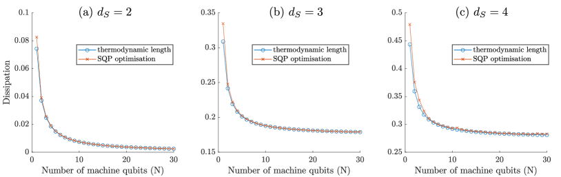
Figure 4: Comparison of the thermodynamic-length protocol with numerical optimisation. We plot the dissipation $\beta\Delta E_{\raisebox{0.0pt}{\tiny{$M$}}}-\widetilde{\Delta}S_{\raisebox{0.0pt}{\tiny{$S$}}}$ as a function of the number of machine qubits $N$ for (a) qubit, (b) qutrit and (c) ququart target systems. While our numerical SQP approach is not guaranteed to yield the optimal solution, we readily see that the values obtained are very close to those of the thermodynamic-length protocol.

In the special case of a qubit target interacting with qubit machines, we can nonetheless analytically prove optimality of the sequence of swap operations, as we now demonstrate.

Qubit-qubit case.—One of the key difficulties in analytically solving this optimisation problem lies in characterising the conditions for which a given transformation $\varrho_{\raisebox{0.0pt}{\tiny{$S$}}}\mapsto\varrho_{\raisebox{0.0pt}{\tiny{$S$}}}^{\prime}$ is possible. Fortunately, for the case of a qubit target interacting with qubit machines $d_{\raisebox{0.0pt}{\tiny{$S$}}}=d_{\raisebox{0.0pt}{\tiny{$M$}}}=2$, we can precisely characterise such states via the following lemma.

Lemma 1 (Refs. [20, 21]).

For given qubit states $\varrho_{\raisebox{0.0pt}{\tiny{$S$}}}$ and $\sigma_{\raisebox{0.0pt}{\tiny{$M$}}}$ such that $\varrho_{\raisebox{0.0pt}{\tiny{$S$}}}\prec\sigma_{\raisebox{0.0pt}{\tiny{$M$}}}$, all achievable marginals from a global unitary evolution $U$ satisfy

$$\frac{\mathbbm{1}}{2}\,\prec\,\mathrm{tr}_{\raisebox{0.0pt}{\tiny{$S/M$}}}[U(\varrho_{\raisebox{0.0pt}{\tiny{$S$}}}\otimes\sigma_{\raisebox{0.0pt}{\tiny{$M$}}})U^{\dagger}]\,\prec\,\sigma_{\raisebox{0.0pt}{\tiny{$M$}}}.$$ (31)

Since any pair of qubit states admits a majorisation relation between them, the above condition fully characterises the set of achievable transformations. Thus, a qubit-to-qubit transformation $\varrho_{\raisebox{0.0pt}{\tiny{$S$}}}=\operatorname{diag}(\lambda,1-\lambda)\mapsto\varrho_{\raisebox{0.0pt}{\tiny{$S$}}}^{\prime}=\operatorname{diag}(\lambda^{\prime},1-\lambda^{\prime})$, where $\lambda^{\prime}\geq\lambda$, is possible via Eq. (26) if and only if

$$\varrho_{\raisebox{0.0pt}{\tiny{$S$}}}^{\prime}\prec\tau_{\raisebox{0.0pt}{\tiny{$M$}}}(\beta,H_{\raisebox{0.0pt}{\tiny{$M$}}}).$$ (32)

There is an entire family of thermal states that majorise $\varrho_{\raisebox{0.0pt}{\tiny{$S$}}}$, namely any that have ground-state population larger than that of the final state; from any of these, one can achieve the desired $\varrho_{\raisebox{0.0pt}{\tiny{$S$}}}^{\prime}$. Given that the target system and machine begin at the same temperature and both of their ground-state energies are set to zero without loss of generality, said family of thermal states is characterised by $\omega_{\raisebox{0.0pt}{\tiny{$M$}}}\geq\omega_{\raisebox{0.0pt}{\tiny{$S$}}}$, where $\omega_{\raisebox{0.0pt}{\tiny{$X$}}}$ denotes the energy gap of the system with Hamiltonian $H_{\raisebox{0.0pt}{\tiny{$X$}}}$.

The question is now reduced to: What is the optimal global operation (in the sense of minimising the dissipated heat) to apply to a thermal machine state of this form in order to achieve the desired transformation? Since creating correlations and coherences both incur energy costs [40, 41, 42], we must consider the parameterised family of probabilistic swap operations, i.e.,

$$U=q\,\mathbb{S}+(1-q)\openone,$$ (33)

where $q\in[0,1]$ and $\mathbb{S}$ and $\openone$ denote the swap and identity operators, respectively. This is the most general form of operations between diagonal states that do not create any correlations or coherences in the marginals. In terms of the vectorised formulation of the problem [see (A.1)], this family of operations corresponds to the matrix

$$A=\left[\begin{array}[]{cccc}1&0&0&0\\ 0&1-q&q&0\\ 0&q&1-q&0\\ 0&0&0&1\end{array}\right].$$ (38)

Let the initial state of the target system correspond to $\vec{\lambda}_{\raisebox{0.0pt}{\tiny{$S$}}}=(\lambda,1-\lambda)$ and that of the machine to $\vec{\mu}_{\raisebox{0.0pt}{\tiny{$M$}}}=(\mu,1-\mu)$, where $\mu=(1+e^{-\beta\omega_{\raisebox{0.0pt}{\tiny{$M$}}}})^{-1}$. The general form of the global vector $\vec{\nu}_{\raisebox{0.0pt}{\tiny{$SM$}}}$ after the probabilistic swap operation is

$$\vec{\nu}^{\,\prime}_{\raisebox{0.0pt}{\tiny{$SM$}}}=\left[\begin{array}[]{c}\lambda\mu\\ (1-q)\lambda(1-\mu)+q(1-\lambda)\mu\\ q\lambda(1-\mu)+(1-q)(1-\lambda)\mu\\ (1-\lambda)(1-\mu)\end{array}\right].$$ (43)

The final ground-state population of the target $\lambda^{\prime}=\vec{\nu}^{\,\prime}_{0}+\vec{\nu}^{\,\prime}_{1}$ is thus

$$\lambda^{\prime}=q\mu+(1-q)\lambda.$$ (44)

The dissipated heat is given by the machine energy gap multiplied by the change in the excited-state population of the machine

$$\Delta E_{\raisebox{0.0pt}{\tiny{$M$}}}=\omega_{\raisebox{0.0pt}{\tiny{$M$}}}(\mu-\mu^{\prime})=\omega_{\raisebox{0.0pt}{\tiny{$M$}}}[\mu-\lambda\mu-q\lambda(1-\mu)-(1-q)(1-\lambda)\mu]=\omega_{\raisebox{0.0pt}{\tiny{$M$}}}[q(\mu-\lambda)]=:\omega_{\raisebox{0.0pt}{\tiny{$M$}}}\Delta p,$$ (45)

where $\Delta p$ represents the population exchanged via the transformation. Note that this quantity, which is a function of both the probability of swapping $q$ and the machine energy gap (implicitly via $\mu$), is fixed by the given initial and final states of the target system. Thus, minimising the energy cost per population exchange for a given transformation $\varrho_{\raisebox{0.0pt}{\tiny{$S$}}}\mapsto\varrho_{\raisebox{0.0pt}{\tiny{$S$}}}^{\prime}$, amounts to minimising $\omega_{\raisebox{0.0pt}{\tiny{$M$}}}$. In other words, the transformation should be implemented using the smallest energy gap in the machine; based on Eq. (31), the smallest gap that permits the desired transformation is precisely $\tau_{\raisebox{0.0pt}{\tiny{$M$}}}(\beta,\omega_{\raisebox{0.0pt}{\tiny{$M$}}})=\tau_{\raisebox{0.0pt}{\tiny{$S$}}}(\beta_{\mathrm{f}},\omega_{\raisebox{0.0pt}{\tiny{$S$}}})$. This gives us the optimal initial state of the machine. It is straightforward to see that the desired transformation of the target system is then obtained via the unitary that performs a complete swap, i.e., $q=1$.

A.2 Coherent-control scenario (explicit geodesic solution for the case of a qubit target system)

We now present the explicit geodesic solution for the case where the system is a qubit (i.e., $d_{\raisebox{0.0pt}{\tiny{$S$}}}=2$). In this case we can parameterise the Hamiltonian from Eq. (23) as $H_{t}=H_{0}+\xi_{t}X$, where $\xi_{t}\in[0,1]$ is a continuous function of $t$ and $X$ is a Hermitian operator. Without loss of generality we can assume $H_{0}$ and $X$ to be of the form

$$H_{0}=0\hskip 10.0pt\textup{and}\hskip 10.0ptX=\begin{bmatrix}0&0\\ 0&1\end{bmatrix},$$ (46)

which greatly simplifies the analysis. Our goal is to find a family of functions $\xi_{t}$ that minimises the thermodynamic-length functional $\mathcal{L}$ from Eq. (22). More specifically, using the parameterisation from Eq. (46), the thermodynamic length $\mathcal{L}$ can be written as

$$\mathcal{L} =\int_{0}^{1}\sqrt{\dot{\xi_{t}}m(\xi_{t})\dot{\xi_{t}}}\,\text{d}t,$$ (47)

where $m(\xi_{t})$ is a metric given by $m(\xi_{t})=\mbox{tr}\left[{X^{2}\tau_{t}(\xi_{t})}\right]-\mbox{tr}\left[{X\tau_{t}(\xi_{t})}\right]^{2}=e^{\beta\xi_{t}}{(1+e^{\beta\xi_{t}})^{-2}}$, where $\tau_{t}(\xi_{t}):=e^{-\beta(H_{0}+\xi_{t}X)}/\mathrm{tr}[e^{-\beta(H_{0}+\xi_{t}X)}]$. The optimal path can now be found by solving the Euler-Lagrange equation

$$\frac{\partial\mathcal{L}}{\partial\xi_{t}}=\frac{\text{d}}{\text{d}t}\frac{\partial\mathcal{L}}{\dot{\xi}_{t}}.$$ (48)

This leads to an equation of the form $\ddot{\xi_{t}}+\Gamma_{t}\dot{\xi}^{2}_{t}=0$, where $\Gamma_{t}$ is a Christoffel symbol. In our case, we can explicitly write

$$\Gamma_{t}=\frac{1}{2m(\xi_{t})}\frac{\partial m(\xi_{t})}{\partial\xi_{t}}.$$ (49)

Using our expression for the metric we can solve the above equation for $\Gamma_{t}$, which leads to $\Gamma_{t}=-\tfrac{1}{2}\tanh(\tfrac{\xi_{t}}{2})$. With this, we can now solve Eq. (48) for $\xi_{t}$, which yields

$$\xi_{t}=2\,\mathrm{arcsinh}\left[\tan\left(\frac{c_{1}(t+c_{2})}{2}\right)\right],$$ (50)

where $c_{1},c_{2}\in\mathbb{R}$ are constants that depend on the boundary conditions of the cooling scheme, i.e., the initial and final temperature of the target system. For concreteness, suppose we choose $\beta$ and $\beta_{\mathrm{f}}$ such that the initial state of the system is given by $\varrho_{\raisebox{0.0pt}{\tiny{$S$}}}=\text{diag}(1-p,p)$ and the final one by $\varrho^{\prime}_{\raisebox{0.0pt}{\tiny{$S$}}}=\text{diag}(1-q,q)$, where $p,q\in[0,1]$. Due to our discretisation, the time parameter is given by $t=i/N$, where $i$ labels the machine qubit $M_{i}$ and $N$ is the total number of machine qubits. In this case, the boundary conditions for the trajectory $\xi_{t}$ are $\xi_{0}=-\frac{1}{\beta}\log\left[\frac{p}{1-p}\right]$ and $\xi_{1}=-\frac{1}{\beta}\log\left[\frac{q}{1-q}\right]$.

Appendix B Incoherent-control scenario (Proof of Theorem 2)

We now move to analyse the previously discussed question with respect to the incoherent-control setting. In contrast to that of coherent control, here all heat and entropy flows occur due to the coupling of the target system to a hot ($H$) and cold ($C$) machine, leading to an energy-conserving transformation overall. Beginning with the joint state $\varrho_{\raisebox{0.0pt}{\tiny{$SC{}H$}}}=\tau_{\raisebox{0.0pt}{\tiny{$S$}}}(\beta)\otimes\tau_{\raisebox{0.0pt}{\tiny{$C$}}}(\beta)\otimes\tau_{\raisebox{0.0pt}{\tiny{$H$}}}(\beta_{\raisebox{0.0pt}{\tiny{$H$}}})$, where $\beta_{\raisebox{0.0pt}{\tiny{$H$}}}\leq\beta$, the induced evolution leads to the output state $\varrho_{\raisebox{0.0pt}{\tiny{$SC{}H$}}}^{\prime}=\widetilde{U}\varrho_{\raisebox{0.0pt}{\tiny{$SC{}H$}}}\widetilde{U}^{\dagger}$, where $[\widetilde{U},H_{\raisebox{0.0pt}{\tiny{$S$}}}+H_{\raisebox{0.0pt}{\tiny{$C$}}}+H_{\raisebox{0.0pt}{\tiny{$H$}}}]$ encodes the conservation of energy.

The efficient incoherent cooling scheme that we present is formalised in Theorem 2 of the main text, which provides a bound for the heat drawn from the hot bath. Additionally, we can make a similar statement for the heat dissipated into the cold bath. The restated theorem below encompasses both results.

Theorem 4.

In the incoherent-control setting, the minimum energy cost for cooling a qudit system with Hamiltonian $H$ from a thermal state $\tau_{\raisebox{0.0pt}{\tiny{$S$}}}(\beta,\,H)$ to $\tau_{\raisebox{0.0pt}{\tiny{$S$}}}(\lambda\beta,H)$, by using particular tripartite (energy-conserving) interactions between the system and two fresh qudit machines at inverse temperature $\beta$ (cold) and $\beta_{\raisebox{0.0pt}{\tiny{$H$}}}\leq\beta$ (hot), respectively, and with arbitrary Hamiltonians with $N$$<\infty$ distinct energy gaps but in the limit of infinite steps, is given by

$$\beta\Delta E_{\raisebox{0.0pt}{\tiny{$C$}}}=\,-(\gamma+1)\,\Delta S_{\raisebox{0.0pt}{\tiny{$S$}}}+\,\frac{(\gamma+1)\beta^{2}}{2N}(\mathcal{L}^{*})^{2}+\gamma\beta\,\Delta E_{\raisebox{0.0pt}{\tiny{$S$}}}+\mathcal{O}(N^{-2}),$$ (51)

where $\gamma:=\frac{\beta_{\raisebox{0.0pt}{\tiny{$H$}}}}{\beta-\beta_{\raisebox{0.0pt}{\tiny{$H$}}}}$, and $\mathcal{L}^{*}$ is the thermodynamic length computed for the optimal trajectory (geodesics) $\{\xi_{i}^{*}(t)\}_{i=1}^{N}$ which is the solution to Eq. (24). Since the protocol considered is energy conserving, one can write $\Delta E_{\raisebox{0.0pt}{\tiny{$C$}}}$ in Eq. (51) in terms of the energy changes of $S$ and $H$, i.e., $\Delta E_{\raisebox{0.0pt}{\tiny{$C$}}}=\,-\Delta E_{\raisebox{0.0pt}{\tiny{$S$}}}-\,\Delta E_{\raisebox{0.0pt}{\tiny{$H$}}}$, from which it follows that

$$\Delta F_{\raisebox{0.0pt}{\tiny{$S$}}}^{\beta}\,+\eta\,\Delta E_{\raisebox{0.0pt}{\tiny{$H$}}}=\,-\frac{\beta}{2N}(\mathcal{L}^{*})^{2}+\mathcal{O}(N^{-2}),$$ (52)

where $\Delta F_{\raisebox{0.0pt}{\tiny{$X$}}}^{\beta}:=\Delta E_{\raisebox{0.0pt}{\tiny{$X$}}}-\beta^{-1}\Delta S_{\raisebox{0.0pt}{\tiny{$X$}}}$ and $\eta:=1-\beta_{\raisebox{0.0pt}{\tiny{$H$}}}/\beta=(\gamma+1)^{-1}$. For qubit target systems interacting with qubit hot and cold machines, the interactions considered are optimal in general.

As a side remark, note that when $\gamma\to 0$, i.e., in the limit of an infinite-temperature hot bath, the result above [namely Eq. (51)] reduces to that of the coherent-control setting [i.e., Eq. (4)]. This reflects the intuition that an infinitely hot bath can be considered to be a source of infinite work. However, even in this limit, there is a crucial distinction between the two settings: it is also important to consider the rate at which the target state is cooled; as $\gamma\to 0$, the cooling speed in the incoherent protocol also goes to zero.

Proof.

We begin with a family of machine Hamiltonians and energy-conserving unitaries that can cool the target system. For the described protocol, we explicitly calculate the energy drawn from the hot bath (and that dissipated into the cold bath), which we then bound in terms of the thermodynamic length. We subsequently demonstrate optimality when all systems are qubits.

In the incoherent-control scenario, no energy-conserving unitary with another single thermal machine can lead to cooling the target [21]. Hence, interactions between at least three systems need to be considered. In general, any incoherent-control unitary $\widetilde{U}$ must satisfy the condition of energy conservation $[\widetilde{U},H_{\raisebox{0.0pt}{\tiny{$S$}}}+H_{\raisebox{0.0pt}{\tiny{$C$}}}+H_{\raisebox{0.0pt}{\tiny{$H$}}}]=0$. In order to satisfy this condition, the interaction Hamiltonian that generates this unitary must commute with the local Hamiltonians. In other words, $\widetilde{U}$ can be decomposed into unitaries $\widetilde{U}=\bigotimes_{k}U_{\text{deg}}^{\raisebox{0.0pt}{\tiny{$(k)$}}}\oplus\mathbbm{1}_{\text{rest}}$ that only act non-trivially in the degenerate subspaces of the total Hamiltonian $H:=H_{\raisebox{0.0pt}{\tiny{$S$}}}+H_{\raisebox{0.0pt}{\tiny{$C$}}}+H_{\raisebox{0.0pt}{\tiny{$H$}}}$. Additionally, for the task of cooling the target, it is worth noting that the local Hamiltonians cannot be chosen arbitrarily. For instance, in the qubit case, choosing the energy gaps $E_{\raisebox{0.0pt}{\tiny{$S$}}}$ and $E_{\raisebox{0.0pt}{\tiny{$C$}}}$ constrains the energy gap of the hot machine to fulfill $E_{\raisebox{0.0pt}{\tiny{$H$}}}=\,|E_{\raisebox{0.0pt}{\tiny{$C$}}}-E_{\raisebox{0.0pt}{\tiny{$S$}}}|$. Otherwise, there is no non-trivial unitary that commutes with the sum of the local Hamiltonians, since there would be no degenerate subspace.

We then consider the following energy structures, where the Hamiltonians of the cold and hot baths are scaled versions of that of the target system,

$$H_{\raisebox{0.0pt}{\tiny{$C_{n}$}}}=\left(\left(\gamma+1\right)\lambda_{n}-\,\gamma\right)H_{\raisebox{0.0pt}{\tiny{$S$}}}\quad\quad\text{and}\quad\quad H_{H_{n}}=\left(\gamma+1\right)\left(\lambda_{n}-1\right)H_{\raisebox{0.0pt}{\tiny{$S$}}}.$$ (53)

For such a structure of machine Hamiltonians, we will consider the specific class of energy-conserving unitaries that can be generated via interaction Hamiltonians of the form

$$\widetilde{H}_{\mathrm{int}}=\sum_{i=0}^{d-2}(|{i,\,i+1,\,i}\rangle\!\langle{i+1,\,i,\,i+1}|+|{i+1,\,i,\,i+1}\rangle\!\langle{i,\,i+1,\,i}|).$$ (54)

The unitaries generated from such interactions act non-trivially on $d-1$ distinct two-dimensional orthogonal subspaces, where the $i^{\textup{th}}$ such subspace is spanned by the vectors $\{|{i,\,i+1,\,i}\rangle_{\raisebox{0.0pt}{\tiny{$SCH$}}},\,|{i+1,\,i,\,i+1}\rangle_{\raisebox{0.0pt}{\tiny{$SCH$}}}\}$. This operation represents an exchange between the subspace of the target system spanned by $\{|{i}\rangle_{\raisebox{0.0pt}{\tiny{$S$}}},|{i+1}\rangle_{\raisebox{0.0pt}{\tiny{$S$}}}\}$ and the virtual subspace of the machine spanned by $\{|{i+1,\,i}\rangle_{\raisebox{0.0pt}{\tiny{$CH$}}},|{i,\,i+1}\rangle_{\raisebox{0.0pt}{\tiny{$CH$}}}\}$. Since such subspaces contain total populations strictly less than one, these exchanges with the virtual machine qubits must be repeated infinitely many times in principle, in order for the excited population $p^{(i+1,i)}_{\raisebox{0.0pt}{\tiny{$CH$}}}$ to be swapped with that of the lower-energy eigenstate of the system $p^{(i)}_{\raisebox{0.0pt}{\tiny{$S$}}}$ [20, 21]. Nonetheless, for a large number of repetitions, the approximation holds true. We refer to a number of repeated swaps between the system and a sequence of identical virtual qubits of the machine as a stage. In this case, the exchange leads to a population increase of $\Delta p_{n}^{(i)}:=p^{(i+1,i)}_{\raisebox{0.0pt}{\tiny{$CH$}}}-p^{(i)}_{\raisebox{0.0pt}{\tiny{$S$}}}$ in the energy level $E_{\raisebox{0.0pt}{\tiny{$S$}}}^{(i)}$. This, in turn, allows us to proceed without tracking the full state evolution of the machines when calculating the energy costs associated with both hot and cold machines at each stage $n$, which only depends upon the initial and final states of the target system rather than the more complicated machine states.

As a result, the energy change of each system and within each subspace at stage $n$ of the cooling procedure is thus

$$\Delta E^{\raisebox{0.0pt}{\tiny{$(i)$}}}_{\raisebox{0.0pt}{\tiny{$S_{n}$}}}=-\omega_{\raisebox{0.0pt}{\tiny{$S$}}}^{\raisebox{0.0pt}{\tiny{$(i)$}}}\Delta p^{\raisebox{0.0pt}{\tiny{$(i)$}}}_{n},\quad\quad\quad\Delta E_{\raisebox{0.0pt}{\tiny{$C_{n}$}}}=\omega_{\raisebox{0.0pt}{\tiny{$C_{n}$}}}^{\raisebox{0.0pt}{\tiny{$(i)$}}}\Delta p^{\raisebox{0.0pt}{\tiny{$(i)$}}}_{n},\quad\quad\quad\Delta E^{\raisebox{0.0pt}{\tiny{$(i)$}}}_{H_{n}}=-\omega_{\raisebox{0.0pt}{\tiny{$H_{n}$}}}^{\raisebox{0.0pt}{\tiny{$(i)$}}}\Delta p^{\raisebox{0.0pt}{\tiny{$(i)$}}}_{n},$$ (55)

where $\omega_{\raisebox{0.0pt}{\tiny{$X$}}}^{\raisebox{0.0pt}{\tiny{$(i)$}}}:=E_{\raisebox{0.0pt}{\tiny{$X$}}}^{\hskip 1.0pt\raisebox{0.0pt}{\tiny{$(i\!+\!1)$}}}-E_{\raisebox{0.0pt}{\tiny{$X$}}}^{\hskip 1.0pt\raisebox{0.0pt}{\tiny{$(i)$}}}$ with $\{E_{\raisebox{0.0pt}{\tiny{$X$}}}^{\hskip 1.0pt\raisebox{0.0pt}{\tiny{$(i)$}}}\}_{i=0}^{d-1}$ are the energy eigenvalues of system $X$ sorted in non-decreasing order, and $\Delta p^{\raisebox{0.0pt}{\tiny{$(i)$}}}_{n}$ is the population exchange between energy levels $i$ and $i+1$ of the system at stage $n$. Combining Eqs. (53) and (55) yields

$$\Delta E^{\raisebox{0.0pt}{\tiny{$(i)$}}}_{\raisebox{0.0pt}{\tiny{$C_{n}$}}}=\left(\left(\gamma+1\right)\lambda_{n}-\,\gamma\right)\Delta E^{\raisebox{0.0pt}{\tiny{$(i)$}}}_{\raisebox{0.0pt}{\tiny{$S_{n}$}}}\quad\quad\text{and}\quad\quad\Delta E^{\raisebox{0.0pt}{\tiny{$(i)$}}}_{\raisebox{0.0pt}{\tiny{$H_{n}$}}}=\left(\gamma+1\right)\left(\lambda_{n}-1\right)\Delta E^{\raisebox{0.0pt}{\tiny{$(i)$}}}_{\raisebox{0.0pt}{\tiny{$S_{n}$}}}.$$ (56)

Now, using the fact that the total energy cost associated with each system can be calculated by summing the energy changes in each subspace, i.e., $\Delta E_{\raisebox{0.0pt}{\tiny{$X_{n}$}}}=\,\sum_{i=0}^{d-1}\,\Delta E^{\raisebox{0.0pt}{\tiny{$(i)$}}}_{\raisebox{0.0pt}{\tiny{$X_{n}$}}}$, at each step, it follows (from energy conservation) that one can calculate both the energy drawn from the hot bath and the heat dissipated into the cold bath for any such cooling procedure in terms of the energy change of the target system itself, i.e., $\Delta E_{\raisebox{0.0pt}{\tiny{$C_{n}$}}}=\left(\left(\gamma+1\right)\lambda_{n}-\,\gamma\right)\Delta E_{\raisebox{0.0pt}{\tiny{$S_{n}$}}}$ and $\Delta E_{\raisebox{0.0pt}{\tiny{$H_{n}$}}}=\left(\gamma+1\right)\left(\lambda_{n}-1\right)\Delta E_{\raisebox{0.0pt}{\tiny{$S_{n}$}}}$.

Thus, we need to determine the final state of the target system after each stage $n$. Based on the type of interaction specified in Eq. (54), we can show that this final state depends on the virtual Gibbs ratios of the virtual machine qubits that non-trivially interact with the target system. The virtual Gibbs ratio associated with subspace $i$ at stage $n$ is given by $g^{\raisebox{0.0pt}{\tiny{$(i)$}}}_{n}:=\frac{p^{(i+1,i)}_{C_{n}H_{n}}}{p^{(i,i+1)}_{C_{n}H_{n}}}=e^{-\beta\lambda_{n}\omega_{\raisebox{0.0pt}{\tiny{$S$}}}^{\raisebox{0.0pt}{\tiny{$(i)$}}}}$, where for instance $p^{(i+1,i)}_{C_{n}H_{n}}$ denotes the population in the subspace associated with $|{i+1,i}\rangle_{\raisebox{0.0pt}{\tiny{$C_{n}H_{n}$}}}$. As the number of repeated interactions between the $i^{\text{th}}$ subspace of the target and that of the machine increases, the virtual Gibbs ratio associated with the target subspace $i$ at stage $n$ will converge accordingly, i.e., $\frac{p^{(i\!+\!1)}_{S_{n}}}{p^{(i)}_{S_{n}}}\to e^{-\beta\lambda_{n}\omega_{\raisebox{0.0pt}{\tiny{$S$}}}^{\raisebox{0.0pt}{\tiny{$(i)$}}}}$. It is finally straightforward to see that the thermal state $\tau(\beta,\lambda_{n}H_{\raisebox{0.0pt}{\tiny{$S$}}})$ satisfies this condition, namely that the Gibbs ratio between each pair of neighbouring energy levels in each stage is given by $e^{-\beta\lambda_{n}\omega_{\raisebox{0.0pt}{\tiny{$S$}}}^{\raisebox{0.0pt}{\tiny{$(i)$}}}}$. It is worth mentioning here that in this protocol, rather than the individual states of both hot and cold machines per se, it is the virtual qubits of the total machine that play the most significant role in the reachable states of the target system and the corresponding energy cost.

For the sake of notational simplicity, we will denote thermal states as $\tau_{n}(\beta):=\tau(\beta,\lambda_{n}H_{\raisebox{0.0pt}{\tiny{$S$}}})$, with the boundary points $\tau_{\raisebox{0.0pt}{\tiny{$N$}}}(\beta):=\tau(\beta,\lambda_{\mathrm{f}}H_{\raisebox{0.0pt}{\tiny{$S$}}})$ and $\tau_{\raisebox{0.0pt}{\tiny{$0$}}}(\beta):=\tau(\beta,H_{\raisebox{0.0pt}{\tiny{$S$}}})$. With this, the energy dissipated into the cold machine can be calculated as

$$\Delta E_{\raisebox{0.0pt}{\tiny{$C$}}} =-\sum_{n=1}^{N}\,\Delta E_{\raisebox{0.0pt}{\tiny{$C_{n}$}}}=-\sum_{n=1}^{N}\,\left(\left(\gamma+1\right)\lambda_{n}-\,\gamma\right)\Delta E_{\raisebox{0.0pt}{\tiny{$S_{n}$}}}\,$$

$$=-\sum_{n=1}^{N}\,\left(\left(\gamma+1\right)\lambda_{n}-\,\gamma\right)\mbox{tr}\left[{H_{\raisebox{0.0pt}{\tiny{$S$}}}\left\{\tau_{n}(\beta)-\tau_{n-1}(\beta)\right\}}\right]$$

$$=-\,\left(\gamma+1\right)\sum_{n=1}^{N}\,\mbox{tr}\left[{\lambda_{n}\,H_{\raisebox{0.0pt}{\tiny{$S$}}}\left\{\tau_{n}(\beta)-\tau_{n-1}(\beta)\right\}}\right]+\,\gamma\,\mbox{tr}\left[{H_{\raisebox{0.0pt}{\tiny{$S$}}}\left\{\tau_{\mathrm{f}}(\beta)-\tau_{\raisebox{0.0pt}{\tiny{$0$}}}(\beta)\right\}}\right]$$

$$=\,\frac{\left(\gamma+1\right)}{\beta}\sum_{n=1}^{N}\,\bigg{\{}D\left(\tau_{n-1}(\beta)\hskip 0.5pt\|\hskip 0.5pt\tau_{n}(\beta)\right)-S\left(\tau_{n}(\beta)\right)+S\left(\tau_{n-1}(\beta)\right)\bigg{\}}+\,\gamma\,\mbox{tr}\left[{H_{\raisebox{0.0pt}{\tiny{$S$}}}\left\{\tau_{\mathrm{f}}(\beta)-\tau_{\raisebox{0.0pt}{\tiny{$0$}}}(\beta)\right\}}\right]$$

$$=\,\frac{\left(\gamma+1\right)}{\beta}\sum_{n=1}^{N}\,D\left(\tau_{n-1}(\beta)\hskip 0.5pt\|\hskip 0.5pt\tau_{n}(\beta)\right)-\frac{\left(\gamma+1\right)}{\beta}\Delta S_{\raisebox{0.0pt}{\tiny{$S$}}}+\,\gamma\,\Delta E_{\raisebox{0.0pt}{\tiny{$S$}}},$$ (57)

where we have made use of $D\left(\varrho\hskip 0.5pt\|\hskip 0.5pt\tau(\beta)\right)=-\beta\left[E(\tau(\beta))-E(\varrho)\right]+S(\tau(\beta))-S(\varrho)$ in the third line.

Similarly, the energy drawn from the hot bath can be calculated as

$$\Delta E_{\raisebox{0.0pt}{\tiny{$H$}}} =\sum_{n=1}^{N}\,\mbox{tr}\left[{H_{\raisebox{0.0pt}{\tiny{$H_{n}$}}}\left(\tau_{n}(\beta)-\tau_{n-1}(\beta)\right)}\right]\,$$

$$=\,\left(\gamma+1\right)\sum_{n=1}^{N}\,\mbox{tr}\left[{(\lambda_{n}-1)\,H_{\raisebox{0.0pt}{\tiny{$S$}}}\left\{\tau_{n}(\beta)-\tau_{n-1}(\beta)\right\}}\right]\,$$

$$=\,\left(\gamma+1\right)\sum_{n=1}^{N}\,\bigg{\{}\mbox{tr}\left[{\lambda_{n}\,H_{\raisebox{0.0pt}{\tiny{$S$}}}\left\{\tau_{n}(\beta)-\tau_{n-1}(\beta)\right\}}\right]\bigg{\}}-\,\left(\gamma+1\right)\,\mbox{tr}\left[{H_{\raisebox{0.0pt}{\tiny{$S$}}}\left\{\tau_{\mathrm{f}}(\beta)-\tau_{\raisebox{0.0pt}{\tiny{$0$}}}(\beta)\right\}}\right]$$

$$=\,-\frac{\gamma+1}{\beta}\sum_{n=1}^{N}\,\bigg{\{}D\left(\tau_{n-1}(\beta)\hskip 0.5pt\|\hskip 0.5pt\tau_{n}(\beta)\right)+S\left(\tau_{n-1}(\beta)\right)-S\left(\tau_{n}(\beta)\right)\bigg{\}}-\,\left(\gamma+1\right)\,\mbox{tr}\left[{H_{\raisebox{0.0pt}{\tiny{$S$}}}\left\{\tau_{\mathrm{f}}(\beta)-\tau_{\raisebox{0.0pt}{\tiny{$0$}}}(\beta)\right\}}\right]$$

$$=\,-\frac{\gamma+1}{\beta}\sum_{n=1}^{N}\,\bigg{\{}D\left(\tau_{n-1}(\beta)\hskip 0.5pt\|\hskip 0.5pt\tau_{n}(\beta)\right)+S\left(\tau_{n}(\beta)\right)-S\left(\tau_{n-1}(\beta)\right)\bigg{\}}-\,\left(\gamma+1\right)\,\mbox{tr}\left[{H_{\raisebox{0.0pt}{\tiny{$S$}}}\left\{\tau_{\mathrm{f}}(\beta)-\tau_{\raisebox{0.0pt}{\tiny{$0$}}}(\beta)\right\}}\right]$$

$$=\,-\frac{\gamma+1}{\beta}\sum_{n=1}^{N}\,\bigg{\{}D(\tau_{n-1}(\beta)\hskip 0.5pt\|\hskip 0.5pt\tau_{n}(\beta))\bigg{\}}-\,\left(\gamma+1\right)\left[\,\mbox{tr}\left[{H_{\raisebox{0.0pt}{\tiny{$S$}}}\left\{\tau_{\mathrm{f}}(\beta)-\tau_{\raisebox{0.0pt}{\tiny{$0$}}}(\beta)\right\}}\right]-\frac{1}{\beta}\left\{S(\tau_{\mathrm{f}}(\beta))-S(\tau_{\raisebox{0.0pt}{\tiny{$0$}}}(\beta))\right\}\right].$$ (58)

Using the definition of free energy, $F_{\raisebox{0.0pt}{\tiny{$X$}}}^{\beta}(\varrho):=E_{\raisebox{0.0pt}{\tiny{$X$}}}(\varrho)-\beta^{-1}S(\varrho)$, Eq. (58) can be written as

$$\Delta F_{\raisebox{0.0pt}{\tiny{$S$}}}^{\beta}\,+\eta\,\Delta E_{\raisebox{0.0pt}{\tiny{$H$}}} =\,-\beta^{-1}\sum_{n=1}^{N}\,D\left(\tau_{n-1}(\beta)\hskip 0.5pt\|\hskip 0.5pt\tau_{n}(\beta)\right),$$ (59)

where $\eta=(\gamma+1)^{-1}$ is the Carnot efficiency.

Using the same methods as in Appendix A, the relative entropy terms in both Eqs. (57) and (58) can be bounded in terms of the thermodynamic length, leading to the expressions stated in Eqs. (51) and (52), respectively, as required.

This provides a protocol for cooling a qudit target with qudit hot and cold machines, for which the energy cost can be calculated exactly. For the specific machine Hamiltonians and interactions considered [see Eqs. (53) and (54)], the thermodynamic length expression is optimal in terms of heat dissipation; this therefore completes the first part of the proof. However, global optimality here is not guaranteed since the family of unitaries from which the protocol is derived only corresponds to a subset of energy-conserving ones. Nonetheless, in the qubit case, the analysis simplifies and the class of unitaries considered indeed covers the full orbit of energy-conserving ones (that do not create coherences, which could only be detrimental). Thus, to complete the proof, we can now finally argue for the general optimality of said cooling procedure when all systems are qubits.

Three qubit case.—Recall that in the coherent-control setting, the state of lowest achievable temperature is obtained by swapping each qubit system with successively colder machine qubits. However, such swaps are prohibited in the incoherent setting as they are not energy conserving. Nonetheless, as mentioned above, here one can swap the system with virtual qubits of the hot-and-cold machines. Since any such subspace has norm strictly less than one, each such swap will lead to the system qubit being at strictly higher temperature than that of the virtual machine qubit. However, in the limit of infinitely many repetitions, the temperature of the system-qubit subspace of interest converges to the virtual temperature of the machine-qubit subspace [20, 21]. As we are interested in finite resources, we assume a finite but sufficiently large number of swaps such that the error is acceptable.

With this in mind, following a similar logic to that presented regarding the coherent-control setting, we assume that the local energy gaps of all qubit systems during interaction stage $n$ are given by

$$E_{\raisebox{0.0pt}{\tiny{$S$}}}=E,\;\;E_{C_{n}}=\lambda_{n}\,E\,\quad\text{and}\quad\,E_{H_{n}}=\,(\lambda_{n}-1)\,E,$$ (60)

where $E\in\mathbb{R}^{+}$. In order to make it possible for the target system to be cooled, the condition $E_{C_{n}}\,>\,E_{\raisebox{0.0pt}{\tiny{$S$}}}$ must be satisfied [21]. In this case, at each stage $n$, the degenerate subspace is spanned by the vectors $\{|{010}\rangle,\,|{101}\rangle\}$, where we write $|{ijk}\rangle:=\,|{i}\rangle_{\raisebox{0.0pt}{\tiny{$S$}}}\otimes|{j}\rangle_{\raisebox{0.0pt}{\tiny{$C$}}}\otimes|{k}\rangle_{\raisebox{0.0pt}{\tiny{$H$}}}$.

We now seek the types of energy-conserving unitaries that can cool the target system given this structure. We assume that the cooling scheme is Markovian in the sense that it can be represented as a collision model with the hot and cold baths being completely reset after each step of controlled evolution. As such, any possible correlations generated between the target and machines cannot be used in the next step and are therefore irrelevant. Moreover, creating correlations and coherences from initially uncorrelated thermal states incurs an energy cost [40, 41, 55, 42]. Since we are seeking the minimum such cost, it follows that we need only consider energy-conserving unitaries that permute the populations of the eigenstates. All possible such unitaries can be generated by Hamiltonians of the following form

$$\widetilde{H}_{\textup{int}}=|{010}\rangle\!\langle{101}|+|{101}\rangle\!\langle{010}|,$$ (61)

since acting with $\widetilde{U}(t)=\,\mathrm{exp}[-i\widetilde{H}_{\textup{int}}\,t]$ does not generate any coherence in the marginals of the output state. It is worth mentioning that cooling in the incoherent-control setting has been investigated completely for different energy-level structures and all energy-conserving unitaries in Ref. [21]. There it was shown that the above energy-level structure and interaction Hamiltonian are the only ones that can cool the target system. In other words, as far as cooling with incoherent control for qubits is concerned it is in general sufficient to consider the combination of machine structure given by Eq. (60) and interactions in Eq. (61). With this in mind we now prove optimality.

Due to the energy-conserving nature of the unitary interaction, if the population of the ground state of the target system is increased by $\Delta p_{n}$, all local energy changes at stage $n$ can be calculated as

$$\Delta E_{S_{n}}=-E_{\raisebox{0.0pt}{\tiny{$S$}}}\Delta p_{n},~{}~{}\Delta E_{C_{n}}=E_{C_{n}}\Delta p_{n},~{}~{}\Delta E_{H_{n}}=-E_{H_{n}}\Delta p_{n},$$ (62)

where the energy change of subsystem $X$ is defined by $\Delta E_{\raisebox{0.0pt}{\tiny{$X$}}}=\,\mbox{tr}\left[{H_{\raisebox{0.0pt}{\tiny{$X$}}}\,(\varrho^{\prime}_{\raisebox{0.0pt}{\tiny{$X$}}}-\,\varrho_{\raisebox{0.0pt}{\tiny{$X$}}})}\right]$. Thus, the energy cost per unit of population exchange only depends upon the energy-level structure; this is a special feature that holds for qubits only and does not extend to higher-dimensional systems and hence represents a roadblock for generalisation. In order to minimise the energy cost of cooling, one should therefore use the smallest available energy gap to cool the target system as much as possible at each stage.

Note that, since such an energy-conserving unitary only acts non-trivially in a (strict) subspace, whose population cannot be unity, its effective operation on $S$ and $CH$ considered as a whole is a partial swap (cf. the full swap with the machine in the coherent-control case). Nonetheless, if such a partial swap is repeated a sufficiently many times, refreshing the hot and cold machines each time, the state of the system converges to that which would be obtained by completely swapping the target with a virtual qubit of the machine, i.e., spanned by the vectors $\{|{01}\rangle_{\raisebox{0.0pt}{\tiny{$CH$}}},|{10}\rangle_{\raisebox{0.0pt}{\tiny{$CH$}}}\}$ [20, 21]. In order to cool the target system to inverse temperature $\beta_{n}:=\frac{E_{n}}{E_{\raisebox{0.0pt}{\tiny{$S$}}}}\beta$ at stage $n$ in the incoherent-control setting, the energy gaps of the cold and hot machines must satisfy $E_{C_{n}}\geq(\gamma+1)E_{n}-\gamma E_{\raisebox{0.0pt}{\tiny{$S$}}}$ and $E_{H_{n}}\geq(\gamma+1)(E_{n}-\,E_{\raisebox{0.0pt}{\tiny{$S$}}})$ , where $\gamma:=\frac{\beta_{\raisebox{0.0pt}{\tiny{$H$}}}}{\beta-\beta_{\raisebox{0.0pt}{\tiny{$H$}}}}(=\eta^{-1}-1)$ (see Appendix F 2 in Ref. [8]). Since the energy cost per population exchange depends linearly upon the energy gaps themselves, it is clear that one must use the smallest gaps possible to cool the system at each step in order to minimise the energy cost. Thus, the optimal machine energy structure at each stage $n$ is given by $E_{C_{n}}=(\gamma+1)E_{n}-\gamma E_{\raisebox{0.0pt}{\tiny{$S$}}}$ and $E_{H_{n}}=(\gamma+1)(E_{n}-\,E_{\raisebox{0.0pt}{\tiny{$S$}}})$.

We now move to focus on optimality of the transformation itself [generated by Hamiltonians of the form given in Eq. (61)]. The diagonal energy-conserving transformations considered here for the qubit case can generally be divided into those that increase the ground-state population of the target and those that decrease it, which respectively correspond to cooling and heating the target system. We will now show that heating up the system at any time cannot help to reduce the energy cost of the cooling process. And since the overall protocol proceeds in a Markovian fashion, this therefore completes the proof.

We proceed by way of contradiction. Consider a qubit target system interacting with fresh qubit hot and cold thermal machines at each time. We assume that each machine can be a qubit system whose energy gap is finite, but we have access to infinitely many copies of them. We claim here that the optimal cooling procedure is to cool the target system at each step. Suppose, for the sake of contradiction, that this is not true and that heating the target at some point can help to reduce the energy cost in reaching a desired state at the end of the protocol.

We begin by assuming that the virtual qubits of the machines are ordered in non-decreasing fashion and that we use the smallest possible gap that permits cooling the target from $\frac{p^{\raisebox{0.0pt}{\tiny{$(n-1)$}}}_{1}}{p^{\raisebox{0.0pt}{\tiny{$(n-1)$}}}_{0}}=e^{-\beta E_{n-1}}$ to $\frac{p^{\raisebox{0.0pt}{\tiny{$(n)$}}}_{1}}{p^{\raisebox{0.0pt}{\tiny{$(n)$}}}_{0}}=e^{-\beta E_{n}}$ in stage $n$. As mentioned above, the system must interact here with a machine whose cold subsystem has an energy gap of at least $E_{\raisebox{0.0pt}{\tiny{$C_{n}$}}}=\,\left(\gamma+1\right)E_{n}-\gamma E_{\raisebox{0.0pt}{\tiny{$S$}}}$. The energy dissipated into the cold bath of this stage is simply the product of the cold-machine energy gap and the population transfer, which leads to $\Delta E_{\raisebox{0.0pt}{\tiny{$C_{n}$}}}/\Delta p_{n}\geq E_{\raisebox{0.0pt}{\tiny{$C_{n}$}}}$ and $\Delta E_{\raisebox{0.0pt}{\tiny{$C_{n}$}}}\geq 0$. In the next stage $n+1$, we will investigate all possible ways of heating up the target via energy-conserving unitaries. Since heating the target is equivalent to cooling the cold machine, it is, a priori possible that such a strategy could lead to a reduced energy cost in the long run.

However, this is not the case, as we now show. In order to cool down the cold machine, the target system must interact with a virtual qubit whose population ratio exceeds $e^{-\beta E_{n}}$. For any such heating of the target to reduce the energy cost, one must show that there exists a choice of energy gaps $E_{\raisebox{0.0pt}{\tiny{$C_{n+1}$}}}$ (and corresponding $E_{\raisebox{0.0pt}{\tiny{$H_{n+1}$}}}$) where $E_{\raisebox{0.0pt}{\tiny{$C_{n+1}$}}}\geq\,E_{\raisebox{0.0pt}{\tiny{$C_{n}$}}}$ and $\Delta E_{\raisebox{0.0pt}{\tiny{$C_{n+1}$}}}/\Delta p_{n+1}=E_{\raisebox{0.0pt}{\tiny{$C_{n+1}$}}}$ such that $\Delta E_{\raisebox{0.0pt}{\tiny{$C_{n+1}$}}}\leq 0$. Intuitively, these constraints imply that the energy cost per population exchange in the cooling stage is lower than that of the heating one. If this were true, then one could extract energy from the cold system via a cyclic process, which contradicts the second law. In the following, we will formally show that it is impossible to find such a process by considering all possible energy-level structures and energy-conserving unitaries on three qubits. We finally conclude that heating the system at any point can only serve to increase the energy cost of the overall protocol, and thus the optimal overall procedure can only be a concatenation of cooling steps.

We proceed on a case-by-case basis.

1. $E_{\raisebox{0.0pt}{\tiny{$X$}}}=E_{\raisebox{0.0pt}{\tiny{$Y$}}}$ where $X,Y\in\,\{S,\,C,\,H\}$: In this case, the degenerate subspace is spanned by $\{|{001}\rangle,\,|{010}\rangle,\,|{100}\rangle\}$. Since $\beta_{\raisebox{0.0pt}{\tiny{$H$}}}\leq\beta$, one can reduce the energy dissipated by the cold machine via a bipartite interaction with the target system at inverse temperature $\beta_{n}=\frac{E_{n}}{E_{\raisebox{0.0pt}{\tiny{$S$}}}}\beta\geq\beta$. Here, the energy transferred to the cold machine per population exchange is determined by $E_{\raisebox{0.0pt}{\tiny{$S$}}}<E_{\raisebox{0.0pt}{\tiny{$C_{n}$}}}$. Thus, the energy cost cannot be reduced.

2. $E_{\raisebox{0.0pt}{\tiny{$C$}}}=\,E_{\raisebox{0.0pt}{\tiny{$S$}}}+\,E_{\raisebox{0.0pt}{\tiny{$H$}}}$: In this case, the degenerate subspace is spanned by $\{|{101}\rangle,\,|{010}\rangle\}$. From Ref. [8], in order to heat up the target system, the energy gap of the cold machine must be $E_{\raisebox{0.0pt}{\tiny{$C_{n+1}$}}}\leq\,\left(\gamma+1\right)E_{n}-\,\gamma\,E_{\raisebox{0.0pt}{\tiny{$S$}}}=\,E_{\raisebox{0.0pt}{\tiny{$C_{n}$}}}$. Thus, the energy cost cannot be reduced.

3. $E_{\raisebox{0.0pt}{\tiny{$C$}}}=\,2E_{\raisebox{0.0pt}{\tiny{$S$}}}=\,2E_{\raisebox{0.0pt}{\tiny{$H$}}}$: In this case, there are three different degenerate subspaces. One of them discussed in case b); the other two degenerate subspaces are spanned by $\{|{001}\rangle,\,|{100}\rangle\}$ and $\{|{011}\rangle,\,|{110}\rangle\}$, respectively. In either case, the system can be heated without interacting with the cold machine (i.e., with only a bipartite interaction with the hot machine), which does not affect the energy dissipated by the cold machine.

4. $E_{\raisebox{0.0pt}{\tiny{$H$}}}=\,E_{\raisebox{0.0pt}{\tiny{$S$}}}+\,E_{\raisebox{0.0pt}{\tiny{$C$}}}$: In this case, the degenerate subspace is spanned by $\{|{110}\rangle,\,|{001}\rangle\}$. Here, if the target is heated, so too is the cold machine. Thus, this setting also cannot help to reduce the energy cost.

We can now conclude that in 3-qubit incoherent-control cooling scenarios, heating up the target system at any point cannot reduce the total energy cost of cooling, and so the optimal process must be a concatenation of cooling steps. ∎

Appendix C Role of correlations in the incoherent-control paradigm

Proof.

(Theorem 3). We start from the strong subadditivity of the von Neumann entropy [57],

$$S_{\raisebox{0.0pt}{\tiny{$SCH$}}}+S_{\raisebox{0.0pt}{\tiny{$S$}}}\leq S_{\raisebox{0.0pt}{\tiny{$SC$}}}+S_{\raisebox{0.0pt}{\tiny{$SH$}}},$$ (63)

where we use the notation $S_{\raisebox{0.0pt}{\tiny{$X$}}}:=S(\varrho_{\raisebox{0.0pt}{\tiny{$X$}}})$. Since we begin with an initially uncorrelated global state, the inequality evaluated on $\varrho_{\raisebox{0.0pt}{\tiny{$SCH$}}}=\tau_{\raisebox{0.0pt}{\tiny{$S$}}}(\beta)\otimes\tau_{\raisebox{0.0pt}{\tiny{$C$}}}(\beta)\otimes\tau_{\raisebox{0.0pt}{\tiny{$H$}}}(\beta_{\raisebox{0.0pt}{\tiny{$H$}}})$ reduces to equality, i.e., $S_{\raisebox{0.0pt}{\tiny{$SCH$}}}^{\raisebox{0.0pt}{\tiny{$0$}}}+S_{\raisebox{0.0pt}{\tiny{$S$}}}^{\raisebox{0.0pt}{\tiny{$0$}}}\,=S_{\raisebox{0.0pt}{\tiny{$SC$}}}^{\raisebox{0.0pt}{\tiny{$0$}}}+S_{\raisebox{0.0pt}{\tiny{$SH$}}}^{\raisebox{0.0pt}{\tiny{$0$}}}$. In addition, since the global evolution is unitary, we have that $\Delta S_{\raisebox{0.0pt}{\tiny{$SCH$}}}=0$, where $\Delta S_{\raisebox{0.0pt}{\tiny{$X$}}}:=S_{\raisebox{0.0pt}{\tiny{$X$}}}^{\prime}-\,S_{\raisebox{0.0pt}{\tiny{$X$}}}^{\raisebox{0.0pt}{\tiny{$0$}}}$. Hence

$$\Delta S_{\raisebox{0.0pt}{\tiny{$S$}}}\leq\Delta S_{\raisebox{0.0pt}{\tiny{$SC$}}}+\Delta S_{\raisebox{0.0pt}{\tiny{$SH$}}},$$ (64)

Writing $I_{\raisebox{0.0pt}{\tiny{$XY$}}}:=I(X\!:\!Y)_{\varrho_{\raisebox{0.0pt}{\tiny{$XY$}}}}=S(\varrho_{\raisebox{0.0pt}{\tiny{$X$}}})+S(\varrho_{\raisebox{0.0pt}{\tiny{$Y$}}})-S(\varrho_{\raisebox{0.0pt}{\tiny{$XY$}}})$ then yields

$$-\Delta S_{\raisebox{0.0pt}{\tiny{$S$}}}\leq-\Delta I_{\raisebox{0.0pt}{\tiny{$SC$}}}-\Delta I_{\raisebox{0.0pt}{\tiny{$SH$}}}+\Delta S_{\raisebox{0.0pt}{\tiny{$C$}}}+\Delta S_{\raisebox{0.0pt}{\tiny{$H$}}}.$$ (65)

By symmetry, the same arguments as above can be used to derive

$$-\Delta S_{\raisebox{0.0pt}{\tiny{$C$}}}\leq-\Delta I_{\raisebox{0.0pt}{\tiny{$SC$}}}-\Delta I_{\raisebox{0.0pt}{\tiny{$CH$}}}+\Delta S_{\raisebox{0.0pt}{\tiny{$S$}}}+\Delta S_{\raisebox{0.0pt}{\tiny{$H$}}},$$ (66)

$$-\Delta S_{\raisebox{0.0pt}{\tiny{$H$}}}\leq-\Delta I_{\raisebox{0.0pt}{\tiny{$SH$}}}-\Delta I_{\raisebox{0.0pt}{\tiny{$CH$}}}+\Delta S_{\raisebox{0.0pt}{\tiny{$S$}}}+\Delta S_{\raisebox{0.0pt}{\tiny{$C$}}}.$$ (67)

Combining Eqs. (65), (66), and (67) then leads to

$$\sum_{\raisebox{0.0pt}{\tiny{$X\!\in\!\{\!S\!,\!C\!,\!H\!\}$}}}\Delta S_{\raisebox{0.0pt}{\tiny{$X$}}}\geq\frac{2}{3}\sum_{\alpha}\Delta I_{\alpha},$$ (68)

where $\alpha\in\{SC,SH,CH\}$. Finally, recall the free-energy difference $\Delta F_{\raisebox{0.0pt}{\tiny{$X$}}}^{\beta}:=\Delta E_{\raisebox{0.0pt}{\tiny{$X$}}}-\beta^{-1}\Delta S_{\raisebox{0.0pt}{\tiny{$X$}}}$. If we consider the total energy change of the entire system as work done on the total system by an external agent, i.e., $W:=-\sum_{\raisebox{0.0pt}{\tiny{$X$}}}\Delta E_{\raisebox{0.0pt}{\tiny{$X$}}}$, then Eq. (68) can be written in the form

$$\sum_{\raisebox{0.0pt}{\tiny{$X\!\in\!\{\!S\!,\!C\!,\!H\!\}$}}}\Delta F_{\raisebox{0.0pt}{\tiny{$X$}}}^{\beta}\leq-W-\frac{2}{3}\beta^{-1}\sum_{\alpha}\Delta I_{\alpha}.$$ (69)

In the incoherent-control scenario, since the total energy is conserved, we have $W=0$. Substituting this into Eq. (69) asserts the claim. ∎