No evidence for anisotropy in galaxy spin directions
Abstract
Modern cosmology rests on the cosmological principle, that on large enough scales the Universe is both homogeneous and isotropic. A corollary is that galaxies’ spin vectors should be isotropically distributed on the sky. This has been challenged by multiple authors for over a decade, with claims to have detected a statistically significant dipole pattern of spins. We collect all publicly available datasets with spin classifications (binary clockwise/anticlockwise), and analyse them for large-angle anisotropies (). We perform each inference in both a Bayesian and frequentist fashion, the former establishing posterior probabilities on the multipole parameters and the latter calculating -values for rejection of the null hypothesis of isotropy (i.e. no power at ). All analysis indicate consistency with isotropy to within . We isolate the differences with contrary claims in the ad hoc or biased statistics that they employ.
keywords:
galaxies: formation – galaxies: fundamental parameters – galaxies: statistics – large-scale structure of Universe1 Introduction
When averaged over sufficiently large scales, the Universe is believed to be described by General Relativity and the Friedmann–Robertson–Walker metric in which all regions of space and all lines of sight from any observer are equivalent. The homogeneity scale appears to be reached at 70 Mpc, in agreement with concordance Cold Dark Matter (CDM) cosmology (Ntelis et al., 2017; Gonçalves et al., 2018; Dias et al., 2023; Gonçalves et al., 2017). The observational evidence for isotropy is somewhat weaker, and in fact several observations suggest that preferred directions do exist in the Universe. These include anomalies in the Cosmic Microwave Background (CMB; most recently Jones et al. 2023), non-negligible multipoles in the large-scale velocity field traced by supernovae (Kalbouneh et al., 2023; Hu et al., 2023), strong bulk flows extending to 100s of Mpc (Watkins et al., 2023) and non-convergence of the rest frames of the CMB and distant matter (Rameez et al., 2018; Migkas et al., 2020; Secrest et al., 2022; Dam et al., 2023; Horstmann et al., 2022; Sorrenti et al., 2023). We must assess carefully whether the fundamental tenets of CDM hold before we can settle into an era of “precision cosmology”.
We investigate here a subset of the claims for anisotropy, namely the putative presence of a dipole in galaxies’ spin directions when viewed from the Milky Way. This is a clean test with few possible systematics: one uses images of low-inclination late-type galaxies to determine (e.g. from the direction of spiral arm winding) whether they are spinning towards or away from us, and then ask whether this binary-valued field projected onto the sky has significant power in multipoles beyond (the monopole). Provided the galaxies are at cosmological distance, power should not be generated at low from tidal torque-like interactions (Barnes & Efstathiou, 1987). If true, this finding would therefore force a rethink of basic cosmology, and may imply that the Universe posessed a net angular momentum in its initial conditions (e.g. Schneider & Célérier 1999; Rodrigues 2008; Battisti & Marcianò 2010).
Over the past 15 years (although see MacGillivray & Dodd 1985a; Iye & Sugai 1991; Sugai & Iye 1995 for earlier related attempts) this test has been performed with various datasets, methods for determining spin direction and statistics for quantifying the anisotropy. Although dominated by a few authors, most studies claim to find a significant dipole (MacGillivray & Dodd 1985b; Longo 2007, 2011; Shamir 2017, 2020a, 2020b, 2020c, 2020d, 2021a, 2021b, 2022a, 2022c, 2022d; McAdam & Shamir 2023b; Shamir 2024). Although Iye & Sugai (1991), Land et al. (2008), Hayes et al. (2017), Tadaki et al. (2020) and Iye et al. (2021) do not, their findings were challenged by Shamir (2023).
We collect all publicly available catalogues for which galaxy spin directions have been estimated, a procedure called “annotation”. We assume these are correct, and question merely the statistics with which this data is interrogated for anisotropy. If we find a dipole we may wonder whether the annotation method suffers from a systematic that causes this, but if we do not find a dipole it is highly unlikely that an existing dipole is hidden by such a systematic. Unlike almost all previous authors we do not use because the data are not Gaussian distributed and hence the assumptions underlying hypothesis testing are invalid. Instead we define a likelihood for each galaxy’s spin as a function of low- multipole parameters (monopole, dipole, quadrupole) and the angle between the galaxy direction and multipole axes. We derive posterior probability distributions on these parameters in a Bayesian analysis and use mock data generated under the assumption of isotropy to test that null hypothesis in a frequentist fashion.
2 Observational Data
We collate all publicly available image data that has been used in the literature to test the isotropy of galaxy spins. Beyond the raw data, this test requires an algorithm to calculate the spin direction of each galaxy (annotation). Any difference in results for fixed data could arise either from the annotation method or the statistics with which the annotated data is tested for anisotropy. Here we accept at face value the annotation of the utilised datasets by other authors, and ask merely whether the statistics of the annotated datasets provide compelling evidence for anisotropy. While the annotations themselves may of course be biased (we refer to the relevant papers for arguments that they are unlikely to be), if they imply isotropy it seems highly unlikely that such biases would hide an underlying anisotropy, which one would expect them if anything to increase.
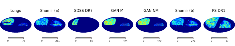
The datasets we use are summarised in Table 1. Most of the datasets (Longo, Shamir(a), SDSS DR7, GAN M, GAN NM and Shamir(b)) come from data releases 6-8 of the Sloan Digital Sky Survey (SDSS; York et al. 2000). PS DR1 derives instead from Pan-STARRS1 (PS1) data release 1 (Chambers et al., 2016). This was was obtained by cross-matching galaxies with identical IDs between two Pan-STARRS datasets, Shamir (2017) and Goddard & Shamir (2020). Thus, this dataset is to our knowledge unique, and no isotropy analysis has previously been conducted on it (although it was annotated in Shamir 2017). The SDSS datasets differ in sky coverage and galaxy density as seen in Figure 1. GAN M is almost identical to GAN NM except the galaxy images were mirrored before being fed into the annotation algorithm, in order to quantify the level of asymmetry in this algorithm. The quoted sigma values in Table 1 were taken from the cited papers, except in the case of (Longo, 2011) where it was calculated from the -value quoted in the abstract of that paper assuming a Gaussian distribution.
Various annotation methods were used. Longo (2011) employed a group of undergraduate students, referred to as “scanners”, to manually annotate randomly assigned redshift slices of the data. The author states that any proclivity for the scanners to prefer a particular spin direction was mitigated by mirroring half of the objects at random to disfavour a particular handedness. The remaining datasets were annotated either by SpArcFiRe (“Scalable Automated Detection of Spiral Galaxy Arm Segments; Davis & Hayes 2014), an algorithm which extracts the structural features of spiral galaxies, or Ganalyzer (“Galaxy Analyzer”), a modelling tool for automated galaxy classification (Shamir, 2011). We investigate the consistency of different annotation methods by cross-matching galaxies with identical IDs between the SDSS-based datasets, finding agreement in spin direction for 91.81% of galaxies matched between Longo and GAN M. As the latter dataset is fully mirrored, this implies that the former is also. This is corroborated by an 8.27% agreement between Longo and GAN NM, and a 93.36% agreement between GAN NM and SDSS DR7. The level of mirroring is however not important for our analysis, which aims simply to investigate the statistical significance for anisotropy from a given set of spin values.
We visualise the datasets in Fig. 1 by plotting the number of galaxies per pixel under a Healpix scheme with nside. We see a significant overlap in area between most of the datasets in the SDSS region. It is clearly imperative for the statistical method used to assess anisotropy to be robust to a highly incomplete sky coverage.
| Name | # gals | Annotation | ||
|---|---|---|---|---|
| Longo | 15158 | 3.16 | Yes | Human scanners |
| Shamir(a) | 72888 | 2.10 | No | Ganalyzer |
| SDSS DR7 | 6103 | — | No | Ganalyzer |
| GAN M | 139852 | 3.97 | Yes | SpArcFiRe, Ganalyzer |
| GAN NM | 138940 | 2.33 | No | SpArcFiRe, Ganalyzer |
| Shamir(b) | 77840 | 2.56 | No | Ganalyzer |
| PS DR1 | 28731 | — | No | Ganalyzer |
3 Method
To ensure that our results are robust to choice of methodology—and suit the taste of the reader—we perform both a Bayesian and frequentist analysis. Each of these rely on a function that describes the likelihood of the data given the model parameters. These parameters, which we denote , are (some subset of) monopole magnitude , dipole magnitude and unit vector direction on the sky , and quadrupole magnitude with corresponding unit sky vectors and . These are multipoles of the on-sky probability field for spins to be clockwise as seen from the Milky Way. We work in equatorial coordinates, where denotes right ascension (RA) and declination (Dec). We denote a galaxy’s spin value as , which we assign the value 0 if the spin is counter-clockwise as seen from the Milky Way, and 1 if it is clockwise. Isotropy therefore corresponds to , and an equal number of clockwise and anticlockwise spins to .
For galaxy , the likelihood function is
| (1) |
where is the unit vector pointing in the direction of the galaxy. This matches the model of Land et al. (2008), and gives the probability that galaxy is spinning in the clockwise direction; the probability that its spin is counter-clockwise is one minus this. We then assume that all galaxies in a dataset are independent, so that the likelihood of the dataset is the product of the likelihood of its constituent galaxies. To investigate how the results are affected by the inclusion of the , and terms we perform separate analyses modelling i) monopole only, ii) dipole only at , iii) monopole and dipole, and iv) monopole, dipole and quadrupole.
3.1 Bayesian analysis
The goal of a Bayesian analysis is to establish posterior probabilities on the model parameters. We adopt uniform priors on , and , and a uniform prior on area element for the , and vectors. This corresponds to a prior uniform in the vector’s RA components and in the cosine of their Dec components. To expedite sampling and eliminate multimodality, we break the symmetry between the two quadrupole vectors by requiring . We also require (there cannot be a negative probability for a galaxy to spin either clockwise or anticlockwise), but never find this to come into play.
We perform a Markov Chain Monte Carlo (MCMC) analysis with the affine-invariant sampler emcee (Foreman-Mackey et al., 2013), using 22 walkers with initial positions randomly sampled from the prior. We calculate the autocorrelation length for each parameter every 100 iterations, terminating when the chain is at least 100 autocorrelation lengths in each parameter and the change in autocorrelation length between iterations is less than 1 per cent.
This produces corner plots describing the posteriors on the parameters and their degeneracies. We summarise each marginal posterior using its mode and 68 per cent confidence interval, unless in which case we instead quote only the 68 per cent upper limit. We assess the goodness-of-fit of each model using the Bayesian Information Criterion (BIC) as an approximation to the Bayesian evidence. This is given by (Schwarz, 1978)
| (2) |
where is the number of free parameters, the number of data points and the maximum-likelihood value. The BIC shows whether the addition of parameters is warranted by the data: an extra parameter must increase the maximum likelihood by at least . As the absolute value is unimportant, we show only differences (BIC) relative to the baseline model inferring only.
3.2 Frequentist analysis
The goal of a frequentist analysis is to calculate a -value for rejection of a null hypothesis, in this case that the Universe is isotropic. First we calculate the maximum-likelihood values of for each dataset using the Nelder–Mead algorithm (Nelder & Mead, 1965; Gao & Han, 2012). Then, for each sample of Table 1, we create 5000 mock datasets with galaxies in the same positions as in the real data but the spins randomised. As we are interested in testing isotropy and not a direction-independent preference for clockwise or counterclockwise spins (which is what a bias in annotation method would naturally produce), the mock data is generated using the maximum-likelihood value, , from the monopole plus dipole model, but . We refit each mock data set to calculate the maximum-likelihood , and then calculate the -value of the null hypothesis as the fraction of mock datasets with more extreme values than the real data. This is done by binning the mock data in the plane and calculating contour levels minimally enclosing fixed fractions of the mock datasets; the contour passing through the real-data point determines the -value. In this case we do not consider a quadrupole.
3.3 Validation
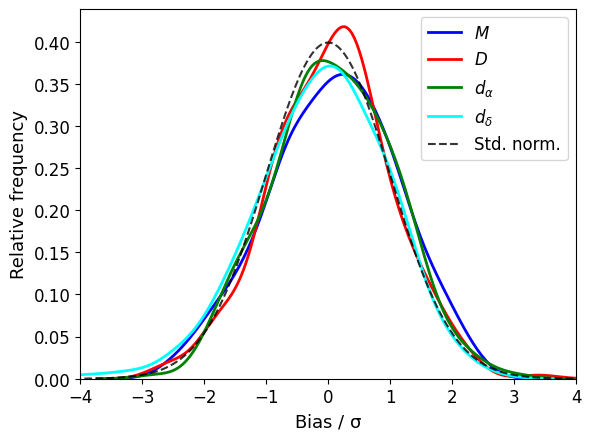
Before applying our method to the real data we validate it on mock data to ensure that it returns unbiased parameter values. Each mock dataset has the same number of galaxies as Shamir(a) (72888), but we generate mock spin values and optionally randomise the positions of the galaxies on the sky. The mock spin values are generated stochastically according to the probabilities corresponding to some true, generating . We calculate a bias value for each parameter and each dataset as
| (3) |
following the Bayesian setup, where angular brackets denote the mean and tilde the true, generating value. This may be interpreted as a discrepancy in between the input parameter value and that recovered by the inference. We find that the distribution of bias values in all cases follows closely the expected standard normal distribution regardless of or the positions of the galaxies on the sky. This is illustrated in Fig. 2 for the case , , , without randomising galaxy positions, over 300 mock datasets.
Note that both of our methods account for the “look-elsewhere effect” that comes into play when testing multiple hypotheses (in this case many possible dipole directions). In the frequentist approach this is accounted for by calculating significance with respect to mock data that has the same properties as the real data and has been processed identically, while in the Bayesian approach it is accounted for by the priors, which appropriately weight the probability that an axis should point in any particular direction.
4 Results
4.1 Bayesian analysis
| Dataset | |
|---|---|
| Longo | |
| Shamir(a) | |
| SDSS DR7 | |
| GAN M | |
| GAN NM | |
| Shamir(b) | |
| PS DR1 |
| Dataset | BIC | |
|---|---|---|
| Longo | 14.8 | |
| Shamir(a) | 0.006 | 22.3 |
| SDSS DR7 | 0.019 | 16.1 |
| GAN M | 0.008 | 41.4 |
| GAN NM | 0.005 | 28.9 |
| Shamir(b) | 0.007 | 20.9 |
| PS DR1 | 16.8 |
| Dataset | BIC | p-value | ||
|---|---|---|---|---|
| Longo | 0.016 | 24.3 | 0.42 | |
| Shamir(a) | 0.005 | 34.0 | 0.32 | |
| SDSS DR7 | 0.046 | 28.0 | 0.65 | |
| GAN M | 0.006 | 35.5 | 0.25 | |
| GAN NM | 0.004 | 35.1 | 0.78 | |
| Shamir(b) | 0.006 | 33.9 | 0.32 | |
| PS DR1 | 20.3 | 0.04 |
| Dataset | BIC | |||
|---|---|---|---|---|
| Longo | 0.023 | 62.1 | ||
| Shamir(a) | 0.005 | < 0.009 | 100 | |
| SDSS DR7 | 0.066 | < 0.090 | 69.5 | |
| GAN M | 0.006 | < 0.010 | 93.3 | |
| GAN NM | 0.004 | < 0.011 | 104 | |
| Shamir(b) | 0.006 | < 0.011 | 92.0 | |
| PS DR1 | 0.021 | 94.4 |
Our results are presented in Tables 2–5. We see that in all cases is consistent with 0.5 within 3 regardless of whether or not one infers or , indicating no significant direction-independent bias in the assignment of clockwise vs anticlockwise spins. Such biases in annotation methods are well documented, for example for visual assessment by citizen scientists in Land et al. (2008); Slosar et al. (2009); Hayes et al. (2017). This may be at play to a minor degree in the Longo and PS DR1 datasets.
When inferring alone, we see a detection of a dipole at just over in the Longo and PS DR1 datasets. The remainder have consistent with 0 at , such that we present only upper limits (and hence there are no meaningful constraints on the dipole direction). These constraints are fairly tight, indicating that a sizeable dipole can be ruled out at high confidence. The positive BIC for all datasets relative to the monopole-only case indicates a worse-fitting model.
From Table 4 we see that it is no coincidence that Longo and PS DR1 have separate monopole and dipole detections: when inferring both and , both Longo anomalies disappear, while those of PS DR1 are reduced in significance, the dipole to almost 2. This illustrates the argument of Land et al. (2008) that degeneracies between and require them to be inferred jointly. The small remaining PS DR1 dipole points towards . Even for PS DR1 the BIC of the monopole+dipole model is , indicating that the inclusion of a dipole is not warranted by the Bayesian evidence. The amount by which any additional parameter must increase the likelihood to be warranted is fairly high due to the large sizes of the datasets.
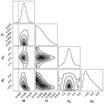
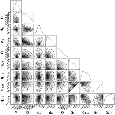
Moving onto Table 5, we see that only the Longo dataset has a non-zero quadrupole at , with direction . This is however not significant at the level. For the other samples the bounds are tight, leading to no significant inflation of the bounds. The BIC values are even larger than for the monopole+dipole model due to the inclusion of a further 5 unwarranted parameters. We show the full corner plots for GAN M, which had the highest claimed dipole significance (Table 1), for the + and ++ analyses in Fig. 3.
To investigate any potential redshift-dependence of the results, we repeat the inference of and for Longo (the only one that provides redshift information) separately for galaxies in the ranges , and . This puts an equal number of galaxies into each tomographic bin. In all cases we find constraints consistent with the full Longo dataset (and the others) that and , and that the posteriors are very similar to the results with the spins randomised.
4.2 Frequentist analysis
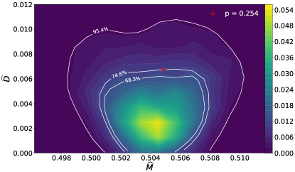
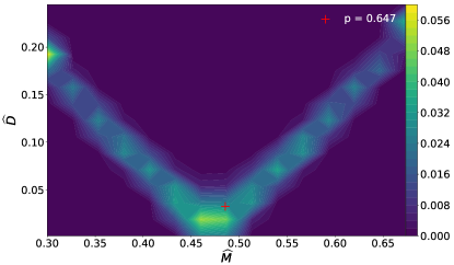
In the final column of Table 4 we show the -value of the null hypothesis of isotropy, calculated using mock data generated according to , (see Sec. 3.2). Only for PS DR1 falls just shy of 0.05, although the BIC still indicates that the monopole-only model is preferred. The frequentist analysis therefore corroborates the Bayesian one that there is no significant evidence for anisotropy. The method is illustrated for GAN M in Fig. 4, in which the distribution of recovered and values on the mock datasets are compared to those of the real data.
It is worth emphasising that the patchy sky coverage of some of our datasets lead to significant parameter degeneracies, which both of our analysis methods naturally account for. In particular, SDSS DR7 consists of a relatively small number of galaxies with poor sky coverage (see Fig. 1), and hence cannot distinguish between a modified monopole and a dipole aligned or antialigned with the observed region. To illustrate the effect of this, we show in Fig. 5 the counterpart of Fig. 4 for this dataset. Our analysis would correctly recover no significant anisotropy even if the best-fit and values in real data were far from and in the degeneracy direction.
4.3 Comparison to the literature
Our clear findings in support of galaxy spin isotropy raise the question of why others have reached diametrically opposite conclusions. To investigate this, we attempt to implement the methods of some such authors on their respective datasets.
The only available mention of a dipole statistic in studies claiming a dipole is eq. 1 of McAdam & Shamir (2023b), which in our notation reads
| (4) |
is the unit dipole axis in the direction. This is evaluated on a grid of for the real data (yielding ) and also of 1000 mock data sets in which the spin directions are randomised (yielding for the mock data set). The significance of the dipole in the direction of is then calculated as
| (5) |
where angled brackets denote a mean over the mock data sets. Eq. 4 appears to be Pearson’s statistic, in which one replaces the squared uncertainty in the denominator of the regular Gaussian by the expected value, in this case corresponding to a dipole magnitude . However, the observed value is , not which mixes the observation with the expectation. This effectively projects onto the dipole axis, which amounts to modelling the expected value as 1 everywhere in the hemisphere aligned with the dipole direction, neglecting the fact that the likelihood of is lower the further one is from the dipole axis, even if the expected value is . Larger discrepancies from the dipole axis may contribute more to the overall chi-squared statistic. Even besides this, we do not consider Eq. 4 a useful statistic because it does not capture the sampling distribution of the observable as do both our Bayesian and frequentist methods. Furthermore, our attempt at using this equation on the McAdam & Shamir (2023b) dataset did not yield the results quoted in that paper, so we were unable to reproduce their analysis. An attempt to reproduce the results of Longo (2011) using Eq. 4 (a shot in the dark, since Longo 2011 do not define their statistic) similarly failed. There do not appear to be any reliable or reproducible results indicating significant anisotropy.
5 Conclusion
We have analysed seven datasets of galaxy sky positions and spin directions to assess the evidence for anisotropy in galaxies’ angular momenta. Four of these datasets have literature claims of a 2 dipole in the spin directions, with two at 3. However, we find clear consistency with statistical isotropy in all datasets using either a Bayesian or frequentist method, both of which account for the look-elsewhere effect and account fully for parameter degeneracies. Due to the incomplete sky coverage spherical harmonics are not orthogonal, leading us to explore the possibility of a quadrupole as well as a dipole and monopole, but this too is small and does not affect our or results. We trace the difference with literature results claiming a dipole to the unmotivated statistics that they employ, and do not find their results to be reproducible.
In conclusion, galaxy spins exhibit large-scale isotropy in adherence to the cosmological principle. Our work highlights the vital importance of careful statistics in analysing fundamental properties of the Universe.
6 Data availability
The annotated galaxy catalogues are available online at the following URLs:
- •
- •
- •
- •
- •
- •
All other data underlying the article will be made available on reasonable request to the authors.
Acknowledgements
We thank Pedro Ferreira, Kazuya Koyama and Sebastian von Hausegger for useful discussions.
DP was supported by a SEPnet Summer Placement at the Institute of Cosmology and Gravitation, University of Portsmouth. HD is supported by a Royal Society University Research Fellowship (grant no. 211046).
This project has received funding from the European Research Council (ERC) under the European Union’s Horizon 2020 research and innovation programme (grant agreement No 693024). For the purpose of open access, we have applied a Creative Commons Attribution (CC BY) licence to any Author Accepted Manuscript version arising.
References
- Barnes & Efstathiou (1987) Barnes J., Efstathiou G., 1987, ApJ, 319, 575
- Battisti & Marcianò (2010) Battisti M. V., Marcianò A., 2010, Phys. Rev. D, 82, 124060
- Chambers et al. (2016) Chambers K. C., et al., 2016, arXiv e-prints, p. arXiv:1612.05560
- Dam et al. (2023) Dam L., Lewis G. F., Brewer B. J., 2023, MNRAS, 525, 231
- Davis & Hayes (2014) Davis D. R., Hayes W. B., 2014, ApJ, 790, 87
- Dias et al. (2023) Dias B. L., Avila F., Bernui A., 2023, Monthly Notices of the Royal Astronomical Society, 526, 3219
- Foreman-Mackey et al. (2013) Foreman-Mackey D., Hogg D. W., Lang D., Goodman J., 2013, PASP, 125, 306
- Gao & Han (2012) Gao F., Han L., 2012, Computational Optimization and Applications, 51, 259
- Goddard & Shamir (2020) Goddard H., Shamir L., 2020, ApJS, 251, 28
- Gonçalves et al. (2017) Gonçalves R. S., Carvalho G. C., Bengaly Jr C. A. P., Carvalho J. C., Bernui A., Alcaniz J. S., Maartens R., 2017, Monthly Notices of the Royal Astronomical Society: Letters, 475, L20
- Gonçalves et al. (2018) Gonçalves R. S., Carvalho G. C., Bengaly C. A. P., Carvalho J. C., Alcaniz J. S., 2018, Monthly Notices of the Royal Astronomical Society, 481, 5270
- Hayes et al. (2017) Hayes W. B., Davis D., Silva P., 2017, MNRAS, 466, 3928
- Horstmann et al. (2022) Horstmann N., Pietschke Y., Schwarz D. J., 2022, A&A, 668, A34
- Hu et al. (2023) Hu J. P., Wang Y. Y., Hu J., Wang F. Y., 2023, arXiv e-prints, p. arXiv:2310.11727
- Iye & Sugai (1991) Iye M., Sugai H., 1991, ApJ, 374, 112
- Iye et al. (2021) Iye M., Yagi M., Fukumoto H., 2021, ApJ, 907, 123
- Jones et al. (2023) Jones J., Copi C. J., Starkman G. D., Akrami Y., 2023, arXiv e-prints, p. arXiv:2310.12859
- Kalbouneh et al. (2023) Kalbouneh B., Marinoni C., Bel J., 2023, Phys. Rev. D, 107, 023507
- Land et al. (2008) Land K., et al., 2008, MNRAS, 388, 1686
- Longo (2007) Longo M. J., 2007, arXiv e-prints, pp astro–ph/0703694
- Longo (2011) Longo M. J., 2011, Physics Letters B, 699, 224
- MacGillivray & Dodd (1985a) MacGillivray H. T., Dodd R. J., 1985a, A&A, 145, 269
- MacGillivray & Dodd (1985b) MacGillivray H. T., Dodd R. J., 1985b, A&A, 145, 269
- McAdam & Shamir (2023a) McAdam D., Shamir L., 2023a, Symmetry, 15, 1190
- McAdam & Shamir (2023b) McAdam D., Shamir L., 2023b, Advances in Astronomy, 2023, 1
- Migkas et al. (2020) Migkas K., Schellenberger G., Reiprich T. H., Pacaud F., Ramos-Ceja M. E., Lovisari L., 2020, A&A, 636, A15
- Nelder & Mead (1965) Nelder J. A., Mead R., 1965, The computer journal, 7, 308
- Ntelis et al. (2017) Ntelis P., et al., 2017, J. Cosmology Astropart. Phys., 2017, 019
- Rameez et al. (2018) Rameez M., Mohayaee R., Sarkar S., Colin J., 2018, MNRAS, 477, 1772
- Rodrigues (2008) Rodrigues D. C., 2008, Phys. Rev. D, 77, 023534
- Schneider & Célérier (1999) Schneider J., Célérier M. N., 1999, A&A, 348, 25
- Schwarz (1978) Schwarz G., 1978, The Annals of Statistics, 6, 461
- Secrest et al. (2022) Secrest N. J., von Hausegger S., Rameez M., Mohayaee R., Sarkar S., 2022, ApJ, 937, L31
- Shamir (2011) Shamir L., 2011, ApJ, 736, 141
- Shamir (2017) Shamir L., 2017, Publ. Astron. Soc. Australia, 34, e044
- Shamir (2020a) Shamir L., 2020a, Open Astronomy, 29, 15
- Shamir (2020b) Shamir L., 2020b, Publ. Astron. Soc. Australia, 37, e053
- Shamir (2020c) Shamir L., 2020c, Astronomische Nachrichten, 341, 324
- Shamir (2020d) Shamir L., 2020d, Ap&SS, 365, 136
- Shamir (2021a) Shamir L., 2021a, Particles, 4, 11
- Shamir (2021b) Shamir L., 2021b, Publ. Astron. Soc. Australia, 38, e037
- Shamir (2022a) Shamir L., 2022a, Journal of Astrophysics and Astronomy, 43, 24
- Shamir (2022b) Shamir L., 2022b, PASJ, 74, 1114
- Shamir (2022c) Shamir L., 2022c, MNRAS, 516, 2281
- Shamir (2022d) Shamir L., 2022d, Advances in Astronomy, 2022, 8462363
- Shamir (2023) Shamir L., 2023, Symmetry, 15, 1704
- Shamir (2024) Shamir L., 2024, arXiv e-prints, p. arXiv:2403.17271
- Slosar et al. (2009) Slosar A., et al., 2009, MNRAS, 392, 1225
- Sorrenti et al. (2023) Sorrenti F., Durrer R., Kunz M., 2023, J. Cosmology Astropart. Phys., 2023, 054
- Sugai & Iye (1995) Sugai H., Iye M., 1995, MNRAS, 276, 327
- Tadaki et al. (2020) Tadaki K.-i., Iye M., Fukumoto H., Hayashi M., Rusu C. E., Shimakawa R., Tosaki T., 2020, MNRAS, 496, 4276
- Watkins et al. (2023) Watkins R., et al., 2023, MNRAS, 524, 1885
- York et al. (2000) York D. G., et al., 2000, AJ, 120, 1579