Wavelet-based resolvent analysis of non-stationary flows

Abstract

This work introduces a formulation of resolvent analysis that uses wavelet transforms rather than Fourier transforms in time. Under this formulation, resolvent analysis may extend to turbulent flows with non-stationary mean states. The optimal resolvent modes are augmented with a temporal dimension and are able to encode the time-transient trajectories that are most amplified by the linearised Navier-Stokes equations. We first show that the wavelet- and Fourier-based resolvent analyses give equivalent results for statistically-stationary flow by applying them to turbulent channel flow. We then use wavelet-based resolvent analysis to study the transient growth mechanism in the logarithmic layer of a turbulent channel flow by windowing the resolvent operator in time and frequency. The computed principal resolvent response mode, i.e. the velocity field optimally amplified by the linearised dynamics of the flow, exhibits the Orr mechanism, which supports the claim that this mechanism is key to linear transient energy growth. We also apply this method to non-stationary parallel shear flows such as an oscillating boundary layer, and three-dimensional channel flow in which a sudden spanwise pressure gradient perturbs a fully-developed turbulent channel flow. In both cases, wavelet-based resolvent analysis yields modes that are sensitive to the changing mean profile of the flow. For the oscillating boundary layer, wavelet-based resolvent analysis produces oscillating principal forcing and response modes that peak at times and wall-normal locations associated with high turbulent activity. For the turbulent channel flow under a sudden spanwise pressure gradient, the resolvent modes gradually realign themselves with the mean flow as it deviates. Wavelet-based resolvent analysis thus captures the changes in the transient linear growth mechanisms caused by a time-varying turbulent mean profile.

1 Introduction

Though turbulent flows are highly chaotic systems, they are very often organised into large-scale energetic structures (Jiménez, 2018). These coherent structures have been observed for wall-bounded flows, jet flows, and flows over wings or other bodies. Since coherent structures are important vehicles of mass and energy, they constitute a popular research topic in a variety of fields include climate sciences and aerodynamics.

In this paper, we focus on the coherent structures present in near-wall turbulence. We note the ubiquity of streamwise streaks near the wall, i.e. regions of low and high velocity elongated in the streamwise direction whose shape, life-cycle, and interactions with the outer flow are studied extensively through experiments and numerical simulations (Klebanoff et al., 1962; Kline et al., 1967; Bakewell & Lumley, 1967; Kim et al., 1971; Blackwelder & Eckelmann, 1979; Smith & Metzler, 1983; Johansson et al., 1987; Robinson, 1991; Adrian, 2007; Smits et al., 2011). These streaks are often described as undergoing a quasi-periodic cycle of formation and breakdown, the drivers of which many works are dedicated to understanding (Landahl, 1980; Butler & Farrell, 1993; Hamilton et al., 1995; Panton, 2001; Chernyshenko & Baig, 2005; Del Alamo & Jimenez, 2006; Jiménez, 2018). The structure of near-wall turbulence has inspired the pursuit of lower-dimensional models, wherein high-dimensional flows are described by the dynamical evolution of large spatial structures. Often, these structures are extracted from spatio-temporal correlations exhibited in experimental or numerical data (Lumley, 1967, 2007; Berkooz et al., 1993; Borée, 2003; Mezić, 2013; Abreu et al., 2020; Tissot et al., 2021).

In contrast to data-driven approaches, many works seek to understand the generation and sustenance of coherent structures through the equations of motion. In the context of wall-bounded turbulence, despite the central role of nonlinearities, linear mechanisms have been proposed as sources of highly-energetic large scale coherent structures (Panton, 2001; Chernyshenko & Baig, 2005; Del Alamo & Jimenez, 2006; Jiménez, 2013; Lozano-Durán et al., 2021). One example is the Orr mechanism (Orr, 1907; Jiménez, 2013), in which the mean shear profile near the wall rotates wall-normal velocity perturbations forward in the streamwise direction and stretches vertical scales; to preserve continuity, wall-normal fluxes and velocity perturbations are intensified. Another linear mechanism that has been studied as a possible energy source for coherent velocity perturbations is lift-up (Hwang & Cossu, 2010), which occurs when wall-normal velocity perturbations transport fluid initially near the wall to regions farther away from the wall, allowing it to be accelerated by the faster mean flow away from the wall. The key role of linear mechanisms in near-wall turbulence has been emphasised in works like Del Alamo & Jimenez (2006) and Pujals et al. (2009), which show that, even after removing the nonlinear term from the perturbation equations, linear transient growth via the mean shear generates the dominant (streaky) structures in wall-bounded turbulence. The numerical experiments in Lozano-Durán et al. (2021) show that turbulence can be sustained in the minimal flow unit even without the nonlinear feedback between the velocity fluctuations and the mean velocity profile. The only exception is when the authors suppress either the aforementioned Orr-mechanism or the push-over mechanism, i.e. the momentum transfer from the spanwise mean shear into the streamwise velocity perturbation, suggesting the prominence of linear transient growth in energising near-wall streaks.

Given these results, it is not entirely surprising that resolvent analysis has been fruitful in the analysis and modeling of near-wall turbulence, despite relying a linearisation of the Navier-Stokes equations (Butler & Farrell, 1993; Farrell & Ioannou, 1998; Jovanović & Bamieh, 2005; McKeon & Sharma, 2010). In resolvent analysis, the Navier-Stokes equations are written as a linear dynamical system for velocity and pressure fluctuations about a mean profile. The nonlinear term, along with any additional exogenous force on the system, are represented as a forcing term acting on this system. The resolvent operator refers to the linear map between the forcing inputs and the flow states. In this linearised setting, without computing the nonlinear terms, we can solve for the input (or forcing) terms that would generate the output trajectories (or responses) with the largest kinetic energy (Jovanović & Bamieh, 2005). This is done in practice by taking a singular value decomposition (SVD) of the discretised resolvent operator: the first right singular mode reveals the inputs to which the linearised equations of motion are most sensitive; the first left singular mode reveals the most amplified outputs, and the first singular value squared yields the kinetic energy amplification. The assumption underpinning this approach is that the optimal structures computed by resolvent analysis will be preferentially amplified by the linear dynamics of the flow, believed to be prominent in near-wall turbulence as discussed previously, and will thus manifest as sustained coherent structures. In the context of wall-bounded turbulent flows, resolvent analysis is successful at identifying streamwise rolls as the most perturbing structures, and streamwise streaks as the most amplified structures (McKeon & Sharma, 2010; Bae et al., 2021).

Since resolvent response modes are expected to figure prominently in the flow, a linear combination of the leading response modes have been used to construct low-dimensional approximations of turbulent flows, including channel and pipe flow (Moarref et al., 2013; Gómez et al., 2016; Beneddine et al., 2017; Illingworth et al., 2018; Arun et al., 2023). This is especially tractable when the singular values decay quickly, and the resolvent operator can be represented by a heavily truncated SVD. Other works have also explored the use of resolvent modes in estimating and predicting flows with sparse measurements. Specifically, a low-rank approximation of the resolvent operator can be used to model correlations between different spatial locations of the flow (Martini et al., 2020; Towne et al., 2020). Moreover, the dynamical relevance of resolvent modes in controlling the fully turbulent flow has been probed (Luhar et al., 2014; Yeh & Taira, 2019; Bae et al., 2021). We highlight the work of Bae et al. (2021), who demonstrate the effectiveness of resolvent modes in transferring energy to coherent near-wall turbulent perturbations within a turbulent minimal channel: by subtracting out the contribution of the leading resolvent forcing mode from the nonlinear term at every time step, the streak-regeneration process is interrupted and buffer layer turbulence is suppressed.

Traditionally, the resolvent operator is formulated after Fourier-transforming the linearised Navier-Stokes in time. This restricts its formulation to statistically-steady and quasi-periodic flows (Padovan et al., 2020). Moreover, the resulting SVD modes will be Fourier modes in time, and cannot represent temporally local effects. However, the linear energy amplification mechanisms that are important to near-wall turbulence, namely the Orr-mechanism, are transient processes. Accounting for transient effects is also important in estimation and control problems. In Martini et al. (2020), time-colouring is employed to improve their estimates, and in Yeh & Taira (2019), which studies flow separation over an airfoil, the resolvent operator is modified to select forcing and responses modes acting on a time scale of interest using the exponential discounting method introduced in Jovanovic (2004). Be it for analysis, estimation or control, resolvent modes capable of encoding time are a potentially valuable extension.

In this work, we propose using a wavelet transform (Meyer, 1992) in time to construct the resolvent operator so that the SVD modes for the newly-formulated resolvent operator are localised in time. Wavelets are indeed functions (in time, for this application) whose mass is concentrated in a subset of their domain. This allows a projection onto wavelets to preferentially capture information centered in a time interval. Each wavelet onto which a function is projected also captures a subset of the Fourier spectrum. Due to their properties, wavelets has been used extensively in fluid mechanics research, particularly spatial wavelets which allow for the analysis of select lengthscales concentrated in a region of interest (Meneveau, 1991; Lewalle, 1993). Temporal wavelet transforms have also been used to decompose turbulent flows. In Barthel & Sapsis (2023), the authors show that high-frequency phenomena upstream over an airfoil are correlated with low-frequency extreme events downstream, and exploit the time-frequency localization in wavelet space to build more robust predictors of these extreme events. Other work has focused on constructing an orthogonal wavelet basis from simulation data to best capture self-similarity in the data (Ren et al., 2021; Floryan & Graham, 2021). An operator-based approach is given in Lopez-Doriga et al. (2023, 2024), in which the authors use a time-resolved resolvent analysis to extract transient structures that are preferentially amplified by the linearised flow; these modes notably exhibit a wavelet-like profile in time. In the context of resolvent analysis, the additional time and frequency localization provided by the wavelet transform will allow us to formulate the flow states and forcing around non-stationary mean profiles. The resolvent modes would thus reflect time-localised changes due to transient events in the mean profile. Moreover, resolvent modes that encode both time and frequency information could help analyze linear amplification phenomena that occurs transiently and that separates forcing and response events in time and/or frequency.

The present work is organised as follows. In §2, we describe traditional Fourier-based resolvent analysis and introduce a wavelet-based formulation. We highlight the properties of the wavelet transform and discuss the choice of wavelet basis; we also discuss the efficiency and robustness of the numerical methods to compute the resolvent modes. In §3, we develop and validate wavelet-based resolvent analysis for a variety of systems, ranging from quasi-parallel wall-bounded turbulent flows to spatio-temporally evolving systems. In §3.1, we establish the equivalence of Fourier- and wavelet-based resolvent analyses for the statistically stationary turbulent channel flow and, in §3.2, we showcase the additional capacity of the wavelet-based resolvent to capture linear transient growth under transient forcing. Specifically, we use the time- and frequency-augmented system to capture the Orr-mechanism in turbulent channel flow. Then we apply wavelet-based resolvent analysis to statistically non-stationary flows in §4, notably the turbulent Stokes boundary layer flow in which the mean oscillates periodically in time (§4.1), as well as a turbulent channel flow subjected to a sudden lateral pressure gradient (§4.2). A preliminary version of this work is published in Ballouz et al. (2023b). Conclusions and a discussion of the results are given in §5.

2 Mathematical formulation

2.1 Fourier-based resolvent analysis

The nondimensional incompressible Navier-Stokes equations are given by

$$\frac{\partial\bar{u}_{i}}{\partial{t}}+\bar{u}_{j}\frac{\partial\bar{u}_{i}}{\partial{x_{j}}}=-\frac{\partial\bar{p}}{\partial x_{i}}+\frac{1}{\Rey}\frac{\partial^{2}\bar{u}_{i}}{\partial{x}_{j}\partial{x}_{j}},\quad\frac{\partial\bar{u}_{i}}{\partial{x_{i}}}=0,$$ (1)

where $\bar{u}_{i}$ is the total velocity (including the mean and the fluctuating component) in the $x_{i}$ direction and $\bar{p}$ is the total pressure. The Reynolds number is given by $\Rey=u^{*}L^{*}/\nu$, where $\nu$ is the kinematic viscosity, and $u^{*}$ and $L^{*}$ are respectively a reference velocity and lengthscale used to nondimensionalise $\bar{u}_{i}$, $x_{i}$, and $t$. Likewise, $\bar{p}$ is nondimensionalised by a reference density $\rho^{*}$ and $u^{*}$. The nondimensionalizations for each of the cases studied in this work are give in table 1. The total velocity can be split into $\bar{u}_{i}=U_{i}+u_{i}$. Here, $U_{i}:=\langle\bar{u}_{i}\rangle$ represents the average over ensembles and homogeneous directions, with $\langle\cdot\rangle$ denoting the averaging operation, and $u_{i}$ is the fluctuating component. Similarly, pressure can be decomposed as $\bar{p}=P+p:=\langle\bar{p}\rangle+p$.

We can split  (1) into equations for the mean and the fluctuating components of the flow

$$\frac{\partial{U_{i}}}{\partial t}+\left\langle\bar{u}_{j}\frac{\partial\bar{u}_{i}}{\partial{x_{j}}}\right\rangle=-\frac{\partial{P}}{\partial{x_{i}}}+\frac{1}{\Rey}\frac{\partial^{2}U_{i}}{\partial{x_{j}}\partial{x_{j}}},\quad\frac{\partial{U_{i}}}{\partial{x_{i}}}=0,$$ (2)

$$\frac{\partial{u_{i}}}{\partial t}+U_{j}\frac{\partial{u_{i}}}{\partial{x_{j}}}+u_{j}\frac{\partial{U_{i}}}{\partial{x_{j}}}=-\frac{\partial{p}}{\partial{x_{i}}}+\frac{1}{\Rey}\frac{\partial^{2}u_{i}}{\partial{x_{j}}\partial{x_{j}}}+f_{i},\quad\frac{\partial{u_{i}}}{\partial{x_{i}}}=0,$$ (3)

where $f_{i}$ is the remaining nonlinear terms in the fluctuating equations. Note that some of the terms in the fluctuating equations may be zero depending on the flow configuration. For example, for a flow that is homogeneous in the $x_{1}$ and $x_{3}$ directions, $\partial U_{i}/\partial x_{1}=\partial U_{i}/\partial x_{3}=0$. The equations above do not have an analytic solution unless in very particular situations and are most commonly solved numerically. Discretizing the fluctuating equations, we get

$$\mathsfbi D_{t}\mathsfbi u_{i}+\mathsfbi U_{j}\mathsfbi D_{j}\mathsfbi u_{i}+\mathsfbi{dU}_{i,j}\mathsfbi u_{j}=-\mathsfbi D_{i}\mathsfbi p+\frac{1}{\Rey}\mathsfbi L\mathsfbi u_{i}+\mathsfbi f_{i},\quad\mathsfbi D_{i}\mathsfbi u_{i}=0,$$ (4)

where $\mathsfbi D_{t}$ is the discrete derivative in time, $\mathsfbi D_{i}$ is the discrete derivative in the $x_{i}$ direction, $\mathsfbi L$ is the discrete Laplacian, $\mathsfbi U_{i}$ is the diagonal matrix whose diagonal terms are $U_{i}$ evaluated at the grid points, and $\mathsfbi{dU}_{i,j}$ denotes the diagonal matrix whose diagonal terms are $\partial U_{i}/\partial x_{j}$ evaluated at the grid points. Each discretised equation is an $N_{t}\times N_{1}\times N_{2}\times N_{3}$-dimensional system, where $N_{t}$ is the temporal resolution, and $N_{i}$ are the spatial resolutions in the $x_{i}$, $i=1,2,3$ directions respectively. The discretised velocity and velocity gradient, $\mathsfbi U_{j}$ and $\mathsfbi{dU}_{i,j}$, are $(N_{t}\times N_{1}\times N_{2}\times N_{3})^{2}$ diagonal matrices. In traditional resolvent analysis, we apply the Fourier transform operator in the homogeneous directions and time to the left of  (4), with $\mathsfbi F_{i}$ and $\mathsfbi F_{t}$ denoting Fourier transforms in the $x_{i}-$direction and time respectively, and $\mathsfbi F$ denoting the full space-time transform. The transformed equations are given by

$$(\mathsfbi F\mathsfbi D_{t}\mathsfbi F^{-1})(\mathsfbi F\mathsfbi u_{i})+(\mathsfbi F\mathsfbi U_{j}\mathsfbi D_{j}\mathsfbi F^{-1})(\mathsfbi F\mathsfbi u_{i})+(\mathsfbi F\mathsfbi{dU}_{i,j}\mathsfbi F^{-1})(\mathsfbi F\mathsfbi u_{j})=\\ -(\mathsfbi F\mathsfbi D_{i}\mathsfbi F^{-1})(\mathsfbi F\mathsfbi p)+\frac{1}{\Rey}(\mathsfbi F\mathsfbi L\mathsfbi F^{-1})(\mathsfbi F\mathsfbi u_{i})+\mathsfbi F\mathsfbi f_{i},\quad(\mathsfbi F\mathsfbi D_{i}\mathsfbi F^{-1})(\mathsfbi F\mathsfbi u_{i})=0,$$ (5)

where $\mathsfbi F^{-1}$ is the inverse transformation, or equivalently

$$\widehat{\mathsfbi D_{t}}\hat{\mathsfbi u}_{i}+\widehat{\mathsfbi U_{j}\mathsfbi D_{j}}\hat{\mathsfbi u}_{i}+\widehat{\mathsfbi{dU}_{i,j}}\hat{\mathsfbi u}_{j}=-\widehat{\mathsfbi D_{i}}\hat{\mathsfbi p}+\frac{1}{\Rey}\hat{\mathsfbi L}\hat{\mathsfbi u}_{i}+\hat{\mathsfbi f}_{i},\quad\widehat{\mathsfbi D_{i}}\hat{\mathsfbi u}_{i}=0.$$ (6)

Note that for an arbitrary matrix $\mathsfbi M$ and vector $\mathsfbi b$, $\widehat{\mathsfbi M}:=\mathsfbi F\mathsfbi M\mathsfbi F^{-1}$ and $\hat{\mathsfbi b}:=\mathsfbi F\mathsfbi b$. For temporally stationary systems, this equation can typically be decoupled for each wavenumber and frequency combination. For example, in the case of channel flow where the flow is homogeneous in the streamwise ($x_{1}$) and spanwise ($x_{3}$) directions and $\mathsfbi F=\mathsfbi F_{1}\mathsfbi F_{3}\mathsfbi F_{t}$, the linear operator can be cast as

$$\left[\begin{array}[]{c}\hat{\mathsfbi u}_{1}\\ \hat{\mathsfbi u}_{2}\\ \hat{\mathsfbi u}_{3}\\ \hat{\mathsfbi p}\end{array}\right]=\hat{\mathsfbi{H}}^{(k_{1},k_{3},\omega)}\left[\begin{array}[]{c}\hat{\mathsfbi f}_{1}\\ \hat{\mathsfbi f}_{2}\\ \hat{\mathsfbi f}_{3}\\ \boldsymbol{0}\end{array}\right],$$ (7)

where the superscript $(k_{1},k_{3},\omega)$ indicates the choice of streamwise and spanwise wavenumbers $k_{1}$ and $k_{3}$, and frequency $\omega$ used in the Fourier transforms. Typically, the singular value decomposition of the linear operator $\hat{\mathsfbi{H}}^{(k_{1},k_{3},\omega)}\in\mathbb{C}^{4N_{2}}\times\mathbb{C}^{4N_{2}}$ is taken to study the left and right singular vectors as response and forcing modes, and the singular values as amplification factors or gains. We denote the principal forcing and response modes by $\boldsymbol{\hat{\phi}}(x_{2})=[\boldsymbol{\hat{\phi}}_{1}^{T},\boldsymbol{\hat{\phi}}_{2}^{T},\boldsymbol{\hat{\phi}}_{3}^{T},\boldsymbol{\hat{\phi}}_{p}^{T}]^{T}$ and $\boldsymbol{\hat{\psi}}(x_{2})=[\boldsymbol{\hat{\psi}}_{1}^{T},\boldsymbol{\hat{\psi}}_{2}^{T},\boldsymbol{\hat{\psi}}_{3}^{T},\boldsymbol{0}^{T}]^{T}$ respectively. For a wall-normal spatial domain $[0,L_{2}]$, the modes are normalised such that

$$[\hat{\phi}]:=\frac{1}{L_{2}}\int_{0}^{L_{2}}|\hat{\phi}|^{2}dx_{2}=1,$$ (8)

$$[\hat{\psi}]:=\frac{1}{L_{2}}\int_{0}^{L_{2}}|\hat{\psi}|^{2}dx_{2}=1,$$ (9)

where we use $[\cdot]=\frac{1}{L_{2}}\int_{0}^{L_{2}}|\cdot|^{2}dx_{2}$ to denote the $x_{2}-$integrated energy.

2.2 Wavelet-based resolvent analysis

2.2.1 Formulation

To account for transient behaviour in the mean flow or the fluctuations, we introduce the wavelet-based resolvent analysis. The benefit of the wavelet transform in time is that it preserves both time and frequency information. The wavelet transform projects a function onto a wavelet basis composed of scaled and shifted versions of a mother function $\varphi(t)$. The transformed function depends on the scale $\alpha$ and shift $\beta$ parameters respectively linked to frequency and time information, whereas the Fourier transform is a function of only frequency.

We propose using a wavelet transform in time $\mathsfbi W_{t}$ while keeping the Fourier transform in homogeneous directions. We denote the total transformation operator (wavelet in time and Fourier in homogeneous directions) as $\mathsfbi W$ and its left inverse operator as $\mathsfbi W^{-1}$, which is also the right inverse for unitary transforms. The inverse operator is well-defined and unique for orthogonal wavelet bases. We can then apply $\mathsfbi W$ on the left of (4), which gives

$$(\mathsfbi W\mathsfbi D_{t}\mathsfbi W^{-1})(\mathsfbi W{\mathsfbi u_{i}})+(\mathsfbi W\mathsfbi U_{j}\mathsfbi D_{j}\mathsfbi W^{-1})(\mathsfbi W{\mathsfbi u_{i}})+(\mathsfbi W\mathsfbi{dU}_{i,j}\mathsfbi W^{-1})(\mathsfbi W\mathsfbi u_{j})=\\ -(\mathsfbi W\mathsfbi D_{i}\mathsfbi W^{-1})(\mathsfbi W\mathsfbi p)+\frac{1}{\Rey}(\mathsfbi W\mathsfbi L\mathsfbi W^{-1})(\mathsfbi W\mathsfbi u_{i})+\mathsfbi W\mathsfbi f_{i},\quad(\mathsfbi W\mathsfbi D_{i}\mathsfbi W^{-1})(\mathsfbi W\mathsfbi u_{i})=0,$$ (10)

or

$$\widetilde{\mathsfbi D_{t}}\tilde{\mathsfbi u}_{i}+\widetilde{\mathsfbi U_{j}\mathsfbi D_{j}}\tilde{\mathsfbi u}_{i}+\widetilde{\mathsfbi{dU}_{i,j}}\tilde{\mathsfbi u}_{j}=-\widetilde{\mathsfbi D_{i}}\tilde{\mathsfbi p}+\frac{1}{\Rey}\tilde{\mathsfbi L}\tilde{\mathsfbi u}_{i}+\tilde{\mathsfbi f}_{i},\quad\widetilde{\mathsfbi D_{i}}\tilde{\mathsfbi u}_{i}=0.$$ (11)

Note that for an arbitrary matrix $\mathsfbi M$ and vector $\mathsfbi b$, $\tilde{\mathsfbi M}:=\mathsfbi W\mathsfbi M\mathsfbi W^{-1}$ and $\tilde{\mathsfbi b}:=\mathsfbi W\mathsfbi b$. These equations can be separated for each spatial wavenumber in the homogeneous direction, and thus the dimension of each linear equation is smaller than the full Navier-Stokes equations. If we choose the transformation in time to be the Fourier transform rather than the wavelet transform, $\alpha$ would represent $\omega$, $\beta$ would be irrelevant, and we would recover the traditional Fourier-based resolvent analysis (McKeon & Sharma, 2010) (if the flow is temporally stationary) or the harmonic resolvent (Padovan et al., 2020) analysis (if the flow is periodic in time). Similar to the Fourier-based resolvent analysis, for flows that are homogeneous in the $x_{1}$– and $x_{3}$–directions, this can be written in matrix form as

$$\left[\begin{array}[]{c}\tilde{\mathsfbi u}_{1}(x_{2},\alpha,\beta)\\ \tilde{\mathsfbi u}_{2}(x_{2},\alpha,\beta)\\ \tilde{\mathsfbi u}_{3}(x_{2},\alpha,\beta)\\ \tilde{\mathsfbi p}(x_{2},\alpha,\beta)\end{array}\right]=\tilde{\mathsfbi{\mathsfbi H}}^{(k_{1},k_{3})}\left[\begin{array}[]{c}\tilde{\mathsfbi f}_{1}(x_{2},\alpha,\beta)\\ \tilde{\mathsfbi f}_{2}(x_{2},\alpha,\beta)\\ \tilde{\mathsfbi f}_{3}(x_{2},\alpha,\beta)\\ \boldsymbol{0}\end{array}\right],$$ (12)

where the wavelet-based resolvent operator $\tilde{\mathsfbi{H}}\in\mathbb{C}^{4N_{t}\times N_{2}}\times\mathbb{C}^{4N_{t}\times N_{2}}$ is defined as

$$\tilde{\mathsfbi{H}}=\left[\left(\tilde{\mathsfbi D}_{t}-\frac{1}{\Rey}\tilde{\mathsfbi L}+\widetilde{\mathsfbi U_{i}\mathsfbi D_{i}}\right)\left(\begin{array}[]{cccc}\mathsfbi I&\boldsymbol{0}&\boldsymbol{0}&\boldsymbol{0}\\ \boldsymbol{0}&\mathsfbi I&\boldsymbol{0}&\boldsymbol{0}\\ \boldsymbol{0}&\boldsymbol{0}&\mathsfbi I&\boldsymbol{0}\\ \boldsymbol{0}&\boldsymbol{0}&\boldsymbol{0}&\boldsymbol{0}\end{array}\right)\right.+\left.\left(\begin{array}[]{cccc}\widetilde{\mathsfbi{dU}}_{1,1}&\widetilde{\mathsfbi{dU}}_{1,2}&\widetilde{\mathsfbi{dU}}_{1,3}&\tilde{\mathsfbi D}_{1}\\ \widetilde{\mathsfbi{dU}}_{2,1}&\widetilde{\mathsfbi{dU}}_{2,2}&\widetilde{\mathsfbi{dU}}_{2,3}&\tilde{\mathsfbi D}_{2}\\ \widetilde{\mathsfbi{dU}}_{3,1}&\widetilde{\mathsfbi{dU}}_{3,2}&\widetilde{\mathsfbi{dU}}_{3,3}&\tilde{\mathsfbi D}_{3}\\ \tilde{\mathsfbi D}_{1}&\tilde{\mathsfbi D}_{2}&\tilde{\mathsfbi D_{3}}&\boldsymbol{0}\end{array}\right)\right]^{-1}.$$ (13)

This formulation allows us to study transient flows using resolvent analysis. We denote the principal forcing and response modes obtained under this formulation by $\boldsymbol{\tilde{\phi}}(x_{2},\alpha,\beta)=(\boldsymbol{\tilde{\phi}}_{1},\boldsymbol{\tilde{\phi}}_{2},\boldsymbol{\tilde{\phi}}_{3},\boldsymbol{\tilde{\phi}}_{p})$ and $\boldsymbol{\tilde{\psi}}(x_{2},\alpha,\beta)=(\boldsymbol{\tilde{\psi}}_{1},\boldsymbol{\tilde{\psi}}_{2},\boldsymbol{\tilde{\psi}}_{3},\boldsymbol{0})$ respectively. We denote their respective inverse wavelet-transforms by $\boldsymbol{\breve{\phi}}(x_{2},t):=\mathsfbi W_{t}^{-1}\boldsymbol{\tilde{\phi}}$ and $\boldsymbol{\breve{\psi}}(x_{2},t):=\mathsfbi W_{t}^{-1}\boldsymbol{\tilde{\psi}}$. These are normalised such that

$$\frac{1}{T}\frac{1}{L_{2}}\int_{0}^{T}\int_{0}^{L_{2}}|\breve{\phi}|^{2}dx_{2}dt=1,$$ (14)

$$\frac{1}{T}\frac{1}{L_{2}}\int_{0}^{T}\int_{0}^{L_{2}}|\breve{\psi}|^{2}dx_{2}dt=1,$$ (15)

where $[0,T)$ represents the temporal domain. We denote the inverse-transforms of the modes to the physical domain by $\boldsymbol{\phi}(x_{1},x_{2},x_{3},t):=\mathsfbi W^{-1}\boldsymbol{\tilde{\phi}}$ and $\boldsymbol{\psi}(x_{1},x_{2},x_{3},t):=\mathsfbi W^{-1}\boldsymbol{\tilde{\psi}}$, repectively.

2.2.2 Wavelet-based resolvent analysis with windowing

We can reformulate a resolvent map between forcing and response at specific time shifts and scales by defining a windowed resolvent operator

$$\left[\begin{array}[]{c}\tilde{\mathsfbi u}_{1}(x_{2},\alpha,\beta)\\ \tilde{\mathsfbi u}_{2}(x_{2},\alpha,\beta)\\ \tilde{\mathsfbi u}_{3}(x_{2},\alpha,\beta)\\ \tilde{\mathsfbi p}(x_{2},\alpha,\beta)\end{array}\right]=\mathsfbi{C}\tilde{\mathsfbi{H}}^{(k_{1},k_{3})}\mathsfbi{B}\left[\begin{array}[]{c}\tilde{\mathsfbi f}_{1}(x_{2},\alpha,\beta)\\ \tilde{\mathsfbi f}_{2}(x_{2},\alpha,\beta)\\ \tilde{\mathsfbi f}_{3}(x_{2},\alpha,\beta)\\ 0\end{array}\right],$$ (16)

where $\mathsfbi{B}$ and $\mathsfbi{C}$ are windowing matrices on the forcing and response modes, respectively (Jeun et al., 2016; Kojima et al., 2020). The windowing matrices select a subset of the full forcing and response states. For example, to select a particular scale and shift parameter $(\alpha_{s},\beta_{s})$ for the forcing mode, we set

$$\mathsfbi{B}=\text{diag}\big{(}\mathbbm{1}(\alpha=\alpha_{s})\mathbbm{1}(\beta=\beta_{s})\big{)},$$ (17)

where $\mathbbm{1}(\cdot)$ is an indicator function. The SVD of the windowed resolvent operator, $\mathsfbi{C}\tilde{\mathsfbi{H}}^{(k_{1},k_{3})}\mathsfbi{B}$, allows us to identify forcing and response modes restricted to a limited frequency and time interval.

2.2.3 Choice of wavelet basis

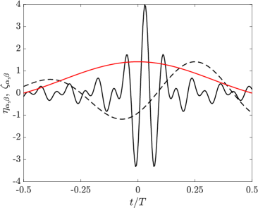
(a)

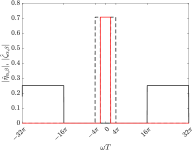
(b)

(c)

(d)

Figure 1: Shannon wavelets and scaling function in time (a) and frequency (b) domains. Daubechies-16 wavelets and scaling function in time (c) and frequency (d) domains. The functions shown are two wavelets for $\alpha=2^{L}=N_{t}$ (black —) and $\alpha=2^{L-3}$ (black $--$), and a scaling function for $\alpha=2^{L}$ (red —).

Wavelet transforms are not unique and are determined by the choice of the mother wavelet $\eta(t)$. The translations and dilations of a real mother wavelet are given by

$$\eta_{\alpha,\beta}(t)\equiv\frac{1}{\sqrt{\alpha}}\eta\left(\frac{t-\beta}{\alpha}\right),$$ (18)

where $\alpha$ and $\beta$ correspond respectively to the scale and shift parameters, and respectively represent location in the frequency and time domains. The dilations of the wavelet capture information at varying scales, and its translations capture information at different time intervals.

Consider an arbitrary function $f(t)$ in $L_{2}(\mathbb{R})$. Its Fourier and wavelet transform are

$$\hat{f}(\omega)=\int_{-\infty}^{+\infty}f(t)e^{-\mathrm{i}\omega t}dt,$$ (19)

$$\tilde{f}^{(w)}(\alpha,\beta)=\int_{-\infty}^{+\infty}f(t)\eta_{\alpha,\beta}(t)dt,$$ (20)

where $\mathrm{i}=\sqrt{-1}$. In practice, we define the wavelet transform on a dyadic grid, i.e. $\alpha=2^{\ell}$, $\beta=k2^{\ell}$ for $k,\;\ell\in\mathbb{Z}$. The dyadic dilations and shifts of the mother wavelet define a complete basis for $L_{2}(\mathbb{R})$. However, we usually do not dilate the mother wavelet indefinitely; the dilations and translations of a scaling function $\zeta(t)$ are used to capture the residual left-over from a scale-truncated wavelet expansion. We define the projection onto these functions as

$$\tilde{f}^{(s)}(\alpha,\beta)=\int_{-\infty}^{+\infty}f(t)\zeta_{\alpha,\beta}(t)dt,\quad\zeta_{\alpha,\beta}(t)\equiv\frac{1}{\sqrt{\alpha}}\zeta\left(\frac{t-\beta}{\alpha}\right).$$ (21)

The wavelet expansion of an arbitrary function $f(t)$ at dyadic scales is thus given by

$$f(t)=\sum_{\ell=-\infty}^{L}\sum_{k=-\infty}^{+\infty}\tilde{f}^{(w)}(2^{\ell},2^{k})\eta\left(\frac{t}{2^{\ell}}-k\right)+\sum_{k=-\infty}^{+\infty}\tilde{f}^{(s)}(2^{L},2^{k})\zeta\left(\frac{t}{2^{L}}-k\right),$$ (22)

where $L\in\mathbb{Z}$ represents the largest scale captured by the wavelet expansion. The $\tilde{f}^{(w)}(2^{\ell},2^{k})$ terms approximate $f(t)$ at scales $-\infty<2^{\ell}\leq 2^{L}$, and the $\tilde{f}^{(s)}(2^{L},2^{k})$ terms capture the residual at scales $2^{\ell}>2^{L}$. In a discretised setting, we use the finite resolution wavelet expansion, which approximates (22) for a discrete signal and where $2\leq 2^{\ell}\leq 2^{L}\leq N_{t}$. The wavelet and scaling function coefficients are produced by a pre-multiplication by $\mathsfbi W_{t}$, which approximates the convolution against the wavelets and scaling functions.

The choice of the wavelet and scaling function pair determines the properties of $\mathsfbi W_{t}$ and thus $\mathsfbi W$. Wavelets/scaling functions of compact support in time result in banded $\mathsfbi W_{t}$, since the convolution with these functions will also have compact support. Orthonormal wavelets/scaling functions result in a unitary $\mathsfbi W_{t}$, making $\mathsfbi W$ unitary as well.

Moreover, each wavelet or scaling function captures a portion of the temporal and frequency domains. There is a trade-off between precision in frequency and precision in time, i.e., one cannot find a function $\eta(t)$ that is well localised in both time and frequency (Mallat, 2001). As two extreme examples, consider the Dirac delta centered at $t=1$, which is perfectly localised in space but with an infinite spread in frequency space, and the Fourier mode $e^{\mathrm{i}t}$, which is perfectly localised in frequency space at $\omega=1$ but has infinite spread in time. In the context of windowed resolvent analysis, we may wish to highlight specific bands of the frequency spectrum, or conversely, narrow bands in time, which will inform the choice of wavelet transform.

For this study, we work with the Shannon and Daubechies-16 wavelets. The Shannon wavelet is notable because it acts as a perfect band-pass filter and covers a frequency band $N_{t}/2^{\ell}([-2\pi,-\pi]\cup[\pi,2\pi])$ (figure 1). Though the Shannon wavelet does not have the perfect frequency localization provided by the Fourier transform, it allows the separation of the frequency content into distinct non-overlapping bands for different scales. One disadvantage of the Shannon wavelet is that it does not have a compact support in time and its corresponding discrete wavelet transform is dense, thus increasing the computational cost of the inversion of $\tilde{\mathsfbi{H}}$ and SVD of its inverse. For problems where the sparsity of the wavelet transform is important, we use the Daubechies wavelets, which trade the perfect band-pass property in frequency domain for a compact support in time. Higher index Daubechies wavelets will have larger temporal supports and will behave closer to perfect band-pass filters. For both the wavelets described, the discrete transform matrix is unitary (Najmi, 2012; Mallat, 2001).

2.2.4 Computational cost

The construction of $\tilde{\mathsfbi{H}}$ requires the inversion of a $4N_{y}N_{t}\times 4N_{y}N_{t}$ matrix, a computation that costs $O(N_{y}^{3}N_{t}^{3})$ operations when solved directly. The full SVD of $\tilde{\mathsfbi{H}}$ would also require $O(N_{y}^{3}N_{t}^{3})$ operations. With a direct solve, the wavelet-based resolvent analysis would cost $O(N_{t}^{2})$-times more than performing $N_{t}$ separate Fourier-based resolvent for each temporal scale, though the latter would fail to capture the interactions between the different time scales. This penalty of $O(N_{t}^{2})$ is the nominal cost of constructing time-localised resolvent modes. Below, we discuss some methods to reduce the cost and memory storage requirements of such a computation.

One method for reducing the memory and computational cost of wavelet-based resolvent analysis is to use sparse finite difference operators and wavelet transforms when constructing $\tilde{\mathsfbi{H}}^{-1}$. We then factor the resulting sparse matrix using specialised packages such as MATLAB’s decomposition, and save the factors in order to later solve linear equations of the form $\tilde{\mathsfbi{H}}^{-1}\mathsfbi v=\mathsfbi w$, where $\mathsfbi v$ and $\mathsfbi w$ are arbitrary vectors, without having to invert $\tilde{\mathsfbi{H}}$ again. This is useful in the context of iterative methods for computing the SVD of $\tilde{\mathsfbi{H}}^{-1}$. Though much of the sparsity of $\tilde{\mathsfbi{H}}$ is lost by the factorization process, we note that the factors still exhibit significant sparsity. In this work, to take advantage of the sparse pre-computed factors of $\tilde{\mathsfbi{H}}$, we opt for an iterative method to perform the SVD. We use a one-sided Lanczos bidiagonalization (Simon & Zha, 2000), which additionally allows us to compute a truncated SVD and accurately estimate a number $q<4N_{y}N_{t}$ of the most significant singular input and output modes.

Other efficient SVD algorithms rely on randomised approaches, in particular by sub-sampling the high-dimensional matrix and performing the SVD on the lower-dimensional approximation (Halko et al., 2011; Drineas & Mahoney, 2016; Tropp et al., 2017). Modifications of randomised SVD algorithms, notably randomised block Krylov methods (Musco & Musco, 2015), have been additionally developed for matrices with slow-decaying singular values, a property exhibited by the resolvent operator in §4.1. A randomised SVD of a high-dimensional discrete resolvent operator was used in Ribeiro et al. (2020) and Yeh et al. (2020).

Another option that would avoid the direct inversion of $\mathsfbi{\tilde{H}}^{-1}$ involves taking the SVD of $\mathsfbi{\tilde{H}}^{-1}$ first. The left and right singular vectors of $\mathsfbi{\tilde{H}}^{-1}$ are respectively the right and left singular vector of $\mathsfbi{\tilde{H}}$. However, since we are looking for the largest singular values of $\mathsfbi{\tilde{H}}$ and their corresponding singular vectors, we would have to compute the full SVD of $\mathsfbi{\tilde{H}}^{-1}$ to find its smallest singular values and corresponding singular vectors. Though this method avoids the inversion of $\mathsfbi{\tilde{H}}^{-1}$, it does not preserve the the efficiency gains of a (heavily) truncated SVD, and should only be used if the sparse factorization of $\mathsfbi{\tilde{H}}^{-1}$ remains the costliest operation. Suppose for example that $\mathsfbi{\tilde{H}}^{-1}$ has $n_{nz}\leq(4N_{y}N_{t})^{2}$ nonzero elements, and that the LU-factorization of $\mathsfbi{\tilde{H}}$ has at most $m_{nz}\leq(4N_{y}N_{t})^{2}$ nonzero elements. Suppose that $n_{nz}$ is small enough that the cost of the LU-factorization is small. A full iterative SVD of $\mathsfbi{\tilde{H}}^{-1}$ has complexity $O(4N_{y}N_{t}n_{nz})$, whereas a $q$-truncated SVD of $\mathsfbi{\tilde{H}}$ has complexity $O(m_{nz}q)$. Thus, if $n_{nz}/m_{nz}<q/(4N_{y}N_{t})$, it is more efficient to compute an SVD of $\mathsfbi{\tilde{H}}^{-1}$ without computing an LU-factorization. For the turbulent Stokes boundary layer problem considered in §3, $q=400$ modes are calculated and $q/(4N_{y}N_{t})\approx 0.001$. Using a second-order finite difference operator in time and Daubechies-8 wavelet transform, $n_{nz}/m_{nz}\approx 0.24$, making the factorization and truncated SVD method more efficient. In general, since we compute a heavily truncated SVD ($q/(4N_{y}N_{t})$ is very small), we find that a factorization of the sparse system prior to the SVD is advantageous.

Resolvent analysis can also be performed more efficiently for the windowed systems described in §2.2.2. Indeed, $\mathsfbi{B}\tilde{\mathsfbi{H}}\mathsfbi{C}=(\mathsfbi{B}^{\dagger}\tilde{\mathsfbi{H}}^{-1}\mathsfbi{C}^{\dagger})^{\dagger}$, where the superscript $\dagger$ indicates the Moore-Penrose pseudo-inverse. Rather than form the resolvent operator $\tilde{\mathsfbi{H}}$ first through an inversion, we can reduce the dimension of the system by windowing the linearised Navier-Stokes operator prior to taking the pseudo-inverse of the windowed system. The matrix pseudo-inversion and SVD will be applied to a lower-dimensional matrix of size defined by the nonzero block of $\mathsfbi{B}\mathsfbi{C}$.

2.2.5 Choice of time differentiation matrix

The choice of the discrete time differentiation operator $\mathsfbi{D}_{t}$ has a significant impact on the computation of resolvent modes. The sparsity of $\mathsfbi{D}_{t}$ controls the sparsity of the resolvent operator, which heavily affects the memory and complexity requirements of the computation of the resolvent modes. However, though a sparse $\mathsfbi{D}_{t}$ seems beneficial, it also distorts the time differentiation for high-frequency waves and can falsify the results of the SVD.

To illustrate this, we study the spectra of two time-derivative matrices, $\mathsfbi D_{t,2}$, a second-order centered finite difference matrix, and $\mathsfbi D_{t,F}$, a Fourier derivative matrix. The eigenvectors of both operators are the discrete Fourier modes. The eigenvalues of the Fourier derivative matrix $\mathsfbi D_{t,F}$ are simply the wavenumbers $\mathrm{i}2\pi k/T$ for $k=1,\,2\,...\lceil{N_{t}/2}\rceil-1$, while those of the second-order centered difference matrix $\mathsfbi D_{t,2}$ are the modified wavenumbers $\mathrm{i}\,\mathrm{sin}(2\pi k/N_{t})N_{t}/T$. For a fixed wavenumber $k$, we note that

$$\lim_{N_{t}\to+\infty}\mathrm{sin}\left(\frac{2\pi k}{N_{t}}\right)\frac{N_{t}}{T}=\frac{2\pi k}{T},$$ (23)

and our modified wavenumber converges to the correct value. Now consider the maximum wavenumer $k=\lceil{N_{t}/2}\rceil-1$. Suppose without loss of generality that $N_{t}$ is even so that $\lceil{N_{t}/2}\rceil-1=N_{t}/2-1$. The limit as the resolution in time increases becomes

$$\lim_{N_{t}\to+\infty}\mathrm{sin}\left(\frac{2\pi}{N_{t}}\left(\frac{N_{t}}{2}-1\right)\right)\frac{N_{t}}{T}=\frac{2\pi}{T},$$ (24)

which does not converge to the correct wavenumber $2\pi(N_{t}/2-1)/T$. Indeed, the error grows as $\mathcal{O}(N_{t})$. Considering an arbitrary matrix $\mathsfbi A$, we can write the following approximation

$$\begin{split}(\mathsfbi D_{t,2}+\mathsfbi A)^{-1}&=(\mathsfbi D_{t,F}+\mathsfbi A+\mathsfbi D_{t,2}-\mathsfbi D_{t,F})^{-1}\\ &\approx(\mathsfbi D_{t,F}+\mathsfbi A)^{-1}-(\mathsfbi D_{t,F}+\mathsfbi A)^{-1}(\mathsfbi D_{t,2}-\mathsfbi D_{t,F})(\mathsfbi D_{t,F}+\mathsfbi A)^{-1}+...\;.\end{split}$$ (25)

Thus,

$$\|(\mathsfbi D_{t,2}+\mathsfbi A)^{-1}-(\mathsfbi D_{t,F}+\mathsfbi A)^{-1}\|_{2}\leq\mathcal{O}(\sqrt{N_{t}})\;\|(\mathsfbi D_{t,F}+\mathsfbi A)^{-1}\|_{2}^{2}+\mathcal{O}(N_{t}).$$ (26)

The lack of convergence as $N_{t}$ increases suggests that the use of a finite difference operator rather than a Fourier derivative can significantly distort the SVD of the resolvent operator. To benefit from the advantages of a sparse temporal finite difference operator while avoiding spurious SVD modes, we propose using the windowing procedure described in §2.2.2 to filter-out the wavelet scales associated with the high-frequency wavenumbers more susceptible to distortion. Specifically, rather than choose the windowing matrices $\mathsfbi B$ and $\mathsfbi C$ to highlight a physically interesting range of the frequency spectrum, we use them to exclude the frequencies above a threshold $k_{\mathrm{max}}<N_{t}/2$. The maximum error between the eigenvalues of $\mathsfbi D_{t,2}$ and $\mathsfbi D_{t,F}$ is given by the Taylor expansion

$$\mathrm{sin}\left(\frac{2\pi k_{\mathrm{max}}}{N_{t}}\right)\frac{N_{t}}{T}-\frac{2\pi k_{\mathrm{max}}}{T}=\frac{4\pi^{3}k_{\mathrm{max}}^{3}}{3N_{t}^{2}T}+\mathcal{O}\left(\frac{k_{\mathrm{max}}^{5}}{N_{t}^{4}}\right).$$ (27)

Thus, assuming the chosen wavelet transform $\mathsfbi W$ is unitary,

$$\|\mathsfbi B\mathsfbi W\left(\mathsfbi D_{t,2}+\mathsfbi A)^{-1}-(\mathsfbi D_{t,F}+\mathsfbi A)^{-1}\right)\mathsfbi W^{-1}\mathsfbi C\|_{2}\leq\mathcal{O}\left(\frac{k_{\mathrm{max}}^{3/2}}{N_{t}}\right)\;\|(\mathsfbi D_{t,F}+\mathsfbi A)^{-1}\|_{2}^{2}.$$ (28)

The error between the SVD of the two operators will decrease as $1/N_{t}$ provided $k_{\mathrm{max}}$ remains fixed. In §3, we employ this filtering approach for cases using a finite difference time derivative operator.

3 Application to statistically-stationary flow

In this section, we first validate wavelet-based resolvent analysis on a statistically-stationary turbulent channel flow, for which the wavelet- and Fourier- approaches are equivalent provided that we use a unitary wavelet transform. Thus, for the channel flow case, we expect the two methods to produce identical resolvent modes. After confirming this result, we exploit the time-localization property of wavelet-based resolvent analysis to study transient growth in turbulent channel flow.

3.1 Turbulent channel flow

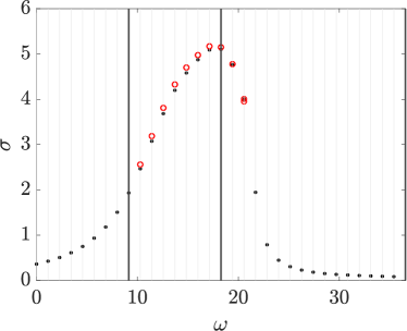
(a)

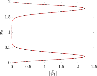
(b)

Figure 2: (a) First ten singular values for the wavelet-based resolvent (red) and the largest singular value of the Fourier-based resolvent operator (black) computed for each $\omega_{i}$. The vertical gray lines indicate the frequencies resolved by the chosen temporal grid, and the vertical black lines delimit the frequency band covered by each of the chosen wavelet scales. (b) Magnitude of $\mathsfbi F\boldsymbol{\psi}_{1}$ (red), the Fourier-transformed principal mode obtained from wavelet-based resolvent analysis, and $\boldsymbol{\hat{\psi}}_{1}$ (black) obtained from traditional Fourier-based resolvent analysis, for $\omega=17.14$, $\lambda_{1}^{+}=1000$ and $\lambda_{3}^{+}=100$.

Case	Section	$L^{*}$	$u^{*}$
Channel flow	§3	$\delta^{*}$ (channel half-height)	$u_{\tau}^{*}$
Turbulent Stokes boundary layer	§4.1	$\delta^{*}_{\Omega}$ (laminar boundary layer thickness)	$U_{\mathrm{max}}^{*}$ (max wall velocity)
Channel flow with spanwise pressure gradient	§4.2	$\delta^{*}$ (channel half-height)	$u_{\tau,0}^{*}$ (wall shear velocity at $t=0$)

Table 1: Length and velocity used to nondimensionalise the Navier-Stokes equations for each case considered in this paper.

The mean profile of turbulent channel flow at friction Reynolds number $\Rey_{\tau}\approx 186$ is obtained from Bae & Lee (2021). We nondimensionalise using the channel half-height $\delta^{*}$ and the friction velocity $u_{\tau}^{*}$ as shown in table 1, so that $\Rey=\Rey_{\tau}$.

For resolvent analysis, the wall-normal direction is discretised using a Chebyshev collocation method using $N_{2}=128$, and the mean streamwise velocity profile and its wall-normal derivative from the DNS are interpolated to the Chebyshev collocation points. We uniformly discretise the temporal domain, $[0,T)$, where $T=5.5$, with a temporal resolution of $N_{t}=128$, and impose periodic boundary conditions at the edges of the time window. The temporal boundary conditions are encoded in the choice of time differentiation matrix $\mathsfbi D_{t}$, which we choose to be a Fourier differentiation matrix. For spatial derivatives in the wall-normal direction, we use first- and second-order Chebyshev differentiation matrices, and impose no-slip and no-penetration boundary conditions at the wall. In choosing $k_{1}$ and $k_{3}$, we target spanwise and streamwise wavelengths of $\lambda_{1}^{+}\approx 1000$ and $\lambda_{3}^{+}\approx 100$ in wall units, which correspond to the most energetic turbulent structures in the near-wall region. Wall units are defined to be $(\cdot)^{+}:=(\cdot)\Rey_{\tau}$ for lengthscales, and $(\cdot)^{+}:=(\cdot)$ for velocity scales. We note that, for this application, the resolvent modes converge despite the relatively low dimension of the resolvent operator. This permits us to use the aforementioned dense differentiation matrices. Sparse finite difference matrices may be used in higher-dimensional problems to improve efficiency.

Since the mean profiles are statistically steady, we have $\widetilde{\mathsfbi U_{j}\mathsfbi D_{j}}=\widehat{\mathsfbi U_{j}\mathsfbi D_{j}}$, $\widetilde{\mathsfbi{dU}_{i,j}}=\widehat{\mathsfbi{dU}_{i,j}}$, and $\tilde{\mathsfbi L}=\hat{\mathsfbi L}$. The wavelet- and Fourier-based cases thus only differ by their time differentiation matrices. These satisfy $\mathsfbi W^{-1}\widetilde{\mathsfbi D_{t}}\mathsfbi W=\mathsfbi F^{-1}\hat{\mathsfbi D_{t}}\mathsfbi F=\mathsfbi D_{t}$. We choose a two-stage Shannon wavelet transform, which is unitary. Thus, since the singular value decomposition is unique up to multiplication by a unitary matrix, we expect the singular values of $\tilde{\mathsfbi H}^{(k_{1},k_{3})}$ to be the same as that of

$$\hat{\mathsfbi{H}}^{(k_{1},k_{3})}=\left(\begin{array}[]{cccc}\hat{\mathsfbi H}^{(k_{1},k_{3},\omega_{1})}&&&\\ &\hat{\mathsfbi H}^{(k_{1},k_{3},\omega_{2})}&&\\ &&\hat{\mathsfbi H}^{(k_{1},k_{3},\omega_{3})}&\\ &&&\ddots\\ \end{array}\right),$$ (29)

where $\omega_{i}=(2\pi i)/T$ for $i=-{N_{t}}/{2},\cdots,{N_{t}}/{2}-1$. Moreover, we expect the response and forcing modes of both systems to be related by the unitary transform given by the Fourier and inverse-wavelet transform in time, $\mathsfbi{FW}^{-1}$.

The results for the Fourier-based cases were computed by applying traditional resolvent analysis at each $\omega_{i}$ captured by our temporal grid, while the wavelet-based resolvent modes were computed by solving the full space-time system at once. As implied by (29), a single wavelet-based resolvent analysis will yield the modes corresponding to all timescales captured by the temporal grid. In order to associate each singular value from the wavelet-based resolvent analysis to a frequency, we Fourier-transform the corresponding response mode in time, and identify the index of the nonzero Fourier component.

In figure 2(a), we show the ten leading singular values of the wavelet-based resolvent operator, along with the first singular value for the Fourier-based operator for different temporal Fourier parameters $\omega_{i}$. The obtained singular values are nearly equal, matching our expectation. The discrepancy can be explained by numerical and truncation errors. Though Shannon wavelet transforms are unitary in the continuous setting, Shannon wavelets do not have compact support in time. The discrete Shannon transform is thus not a unitary matrix due to the truncation of the wavelet in time, and exhibits a condition number of approximately $1.6$ in this case. Using wavelets that are compactly-supported in time, such as the Daubechies wavelets, reduces the discrepancy. Furthermore, increasing the time resolution also reduces the gap between the singular values. We note that due to the symmetry of the problem about the centreline, the singular values appear in equal pairs (McKeon & Sharma, 2010). This is visible in figure 2(a) for $\omega=20.56$, where the pair of singular values deviate slightly for each other due to numerical error. The modes corresponding to the pair of equivalent singular values are reflections of each other about the channel centreline.

In figure  2(b), we plot the streamwise component of the most amplified resolvent response mode for the two methods. For the Fourier-based method, this corresponds to the frequency $\omega\approx 17.14$. For the wavelet-based method, we must first Fourier-transform the principal mode in time. We observe that that the term Fourier modes associated with $\omega\approx 17.14$ is the only nonzero component. Moreover, figure 2(b) shows that the modes from the two methods match. Despite the slight discrepancy in the singular values, both methods yield the same resolvent modes associated with the maximum singular value, indicating that both methods are equivalent for this stationary case.

3.2 Transient growth mechanism of turbulent channel flow

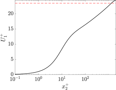
Figure 3: Mean streamwise velocity profile for channel flow at $\Rey_{\tau}=2000$. The dashed line corresponds to the upper bound of the frequency band covered by the chosen wavelet, mapped to streamwise velocities using $U_{1}=\omega/k_{1}$.

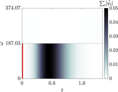
(a)

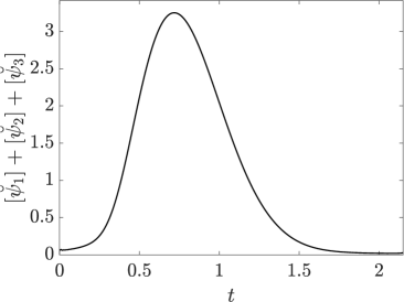
(b)

Figure 4: (a) Inverse wavelet-transformed principal response mode for channel flow at $\Rey_{\tau}=2000$ and $k_{1}=k_{3}\approx 8.98$ under windowed forcing, in the frequency-time plane. The forcing window is highlighted in red. (b) $x_{2}$-integrated total energy of the inverse wavelet-transformed principal response mode.

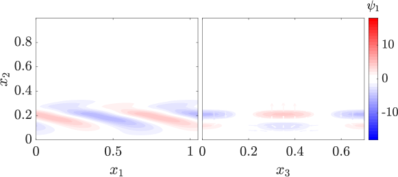
(a)

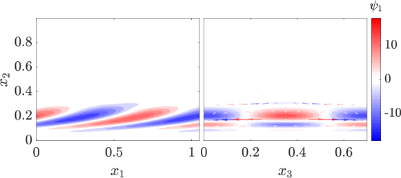
(b)

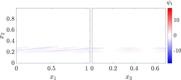
(c)

Figure 5: Principal response mode for the channel flow at $\Rey_{\tau}=2000$ and $k_{1}=k_{3}\approx 8.98$ under transient forcing. The modes are shown at (a) $t=0.25$, (b) $t=0.71$, and (c) $t=1.56$. The left and right panels respectively correspond to half-wavelength locations of $x_{3}/\delta=\pi/k_{3}\delta$ and $x_{1}/\delta=\pi/k_{1}\delta$. The arrows in the right panels are colored according to $\sqrt{|\psi_{2}|^{2}+|\psi_{3}|^{2}}\mathrm{sgn}(\psi_{1})$ to show the intensity of the streamwise rolls relative to the streamwise streaks.

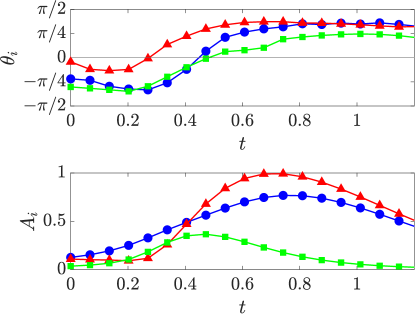
(a)

Figure 6: Mode angle (top) and magnitude (bottom) of the principal response mode as a function of time The streamwise component of the mode is represented by $-\bullet$ (blue), the wall-normal component by $-\blacksquare$ (green) and the spanwise component by $-\blacktriangle$ (red)

The added advantage of the wavelet-based method lies in its ability to preserve temporal localization. The states in (16) encode time and frequency information, which allows us to study transient problems even when the mean profile is statistically stationary. One such transient phenomenon is the Orr mechanism, a linear mechanism first described by Orr (1907) that has been proposed to explain transient energy amplification in shear flows (Jiménez, 2013, 2015; Landahl, 1975; Jiménez, 2018; Encinar & Jiménez, 2020). A two-dimensional physical description is given in Jiménez (2013, 2018): the mean shear profile rotates backward-tilting velocity structures forward (in the positive $x_{1}-$ direction), effectively extending the wall-normal distances between structures; to compensate, continuity will impose larger wall-normal fluxes, i.e. larger wall-normal velocity perturbations. This effect amplifies the velocity perturbations until the velocity structures are tilted past the normal to the wall, after which the mechanism is reversed and the perturbations are attenuated. The Orr mechanism in linearised wall-bounded flows has been examined in Jiménez (2013, 2015, 2018) and Encinar & Jiménez (2020). These studies rely on computing optimal growth trajectories defined as the trajectories emanating from the optimal initial condition which maximises the growth of kinetic energy under the linearised dynamics (Butler & Farrell, 1993; Schmid et al., 2002). These optimal trajectories exhibit the characteristic forward tilting of velocity structures in conjunction with the transient amplification of velocity perturbations, suggesting that the Orr-mechanism is a dominant energy amplification mechanism in the linearised system. Optimal growth trajectories compute the singular modes for the linearised flow map between an initial condition and velocity perturbations at a later time; the question we wish to answer is whether optimal external forcing upon the linearised system, which could originate from nonlinear interactions, also exploits the Orr mechanism. For this, we use the wavelet-based resolvent analysis formulation. We note that traditional resolvent analysis has been used to reveal some evidence of the Orr mechanism in turbulent jets, where it is identified by the tilt of the optimal forcing structures against the jet shear (Pickering et al., 2020; Tissot et al., 2017; Schmidt et al., 2018).

In an attempt to capture the Orr mechanism in channel flow at $Re_{\tau}=2000$ as in Encinar & Jiménez (2020), we use the mean profile for channel flow at $Re_{\tau}=2000$ (Hoyas & Jiménez, 2008), the same grid in the wall-normal direction as §3.1, and a uniform temporal grid with $N_{t}=256$. As argued in Encinar & Jiménez (2020), we choose spatial wavelengths $\lambda_{1}=\lambda_{3}=0.7$, and we choose a total time of $T=2.51$. For this application, we use the Shannon wavelet transform.

To localise our forcing term, we use the windowed wavelet-based resolvent analysis framework from §2.2.2. We set $\mathsfbi{C}$ to the identity matrix, allowing the response modes to cover the entire time and frequency range. We choose $\mathsfbi B$ to restrict the forcing to one of the Shannon wavelets. Without loss of generality, we select the shift parameter $\beta=0$ so that the forcing term is concentrated at a time interval centered at $t=0$. We must also select the scale $\alpha$, which determines the band of frequencies covered by the chosen Shannon wavelet. From traditional resolvent analysis applied to turbulent stationary channel flow, we know that the resolvent Fourier modes tend to peak in magnitude at the critical layer, i.e. where $U(x_{2})=\omega/k_{1}$ (Schmid et al., 2002; McKeon & Sharma, 2010; McKeon, 2017, 2019). In this section, we study the effect of a time-localised forcing on a region $x_{2}^{+}\in[0,500]$ which contains the inner region of the boundary layer (Hoyas & Jiménez, 2006). This maps to a frequency interval $[0,U(x_{2}^{+}=500)]k_{1}=[0,\omega_{\max}]=[0,186.76]$ according to the mean profile for turbulent channel flow (figure 3). Thus we select $\alpha=2$ so that the Shannon wavelet onto which we project the forcing term covers the frequency interval $N_{t}/(2T)[-\pi,\pi]\approx[-187,187]$. The principal resolvent response mode obtained from the SVD of $\tilde{\mathsfbi H}\mathsfbi B$ represents the maximally amplified response to a transient forcing term aligned with the selected wavelet, under the dynamics of the linearised Navier-Stokes.

The resulting principal response mode is confined to the frequency band determined by the forcing, as shown in figure 4(a), which is expected since the time scales are decoupled in resolvent analysis for statistically stationary flows (29). We observe that the spatially integrated energy of the response mode first grows transiently, peaks at $t=0.72$, then decays, as shown in figure 4(b). This transient growth can be explained by the non-normality of the linearised system (Schmid et al., 2002). The response modes at three different times are shown in figure 5. The streamwise component of the modes dominate, and the modes form alternating low- and high-speed streamwise streaks. The shape of the modes is thus in line with previous analysis of the self-sustaining process of wall turbulence (Jiménez & Moin, 1991; Hamilton et al., 1995; Jiménez & Pinelli, 1999; Waleffe, 1997; Schoppa & Hussain, 2002; Farrell et al., 2017; Bae et al., 2020).

In addition to their spatial structure, the transient behaviour of the modes displays characteristics of the Orr mechanism, mainly a synchronisation between the amplification of the response mode and the forward tilting of the velocity structures exhibited by the mode. To study the forward tilting of velocity structures in the response mode, we define the tilt angles as in Jiménez (2015), i.e.

$$\theta_{i}(x_{2},t)=-\mathrm{tan}^{-1}\left(\frac{\partial_{x_{2}}\angle\boldsymbol{\breve{\psi}}_{i}(x_{2},t)}{k_{1}}\right),$$ (30)

where $\angle(\cdot)$ represents the complex angle. In Jiménez (2015), the angle defined above is averaged over a region of interest. We define the energy-weighted average tilt as

$$\theta_{i}^{[y^{+}_{a},y^{+}_{b}]}(t)=\int_{y_{a}}^{y_{b}}\|\boldsymbol{\breve{\psi}}_{i}\|^{2}\theta_{i}dx_{2}/\int_{y_{a}}^{y_{b}}\|\boldsymbol{\breve{\psi}}_{i}\|^{2}dx_{2},$$ (31)

and the amplitude as

$$A_{i}^{[y^{+}_{a},y^{+}_{b}]}=\int_{y_{a}}^{y_{b}}\|\boldsymbol{\breve{\psi}}_{i}\|^{2}dx_{2},$$ (32)

and pick $y_{a}^{+}=0$ and $y_{b}^{+}=2000$ to capture the half-channel. The results (figure 6) show that the amplitude of the wall-normal velocity component of $\boldsymbol{\breve{\psi}}_{2}$ indeed peaks roughly when $\theta^{[0,2000]}_{2}\approx 0$, at $t\approx 0.45$. Moreover, this peak in the wall-normal component triggers peaks in the streamwise and spanwise components at $t\approx 0.75$, possibly through the lift-up mechanism (Encinar & Jiménez, 2020; Jiménez, 2018). The magnitude of the wall-normal component decreases smoothly past $\theta_{2}^{[0,2000]}=0$, until it disappears for $\theta_{2}^{[0,2000]}=\pi/4$. The streamwise and spanwise components also start to collapse at $\theta_{1}^{[0,2000]}=\theta_{3}^{[0,2000]}=\pi/4$. We also note that the transient growth and decay of the wall-normal component of principal response mode occurs at a fast timescale, on the order of $t=1$ , which suggests that the Orr-mechanism can be relevant in the context of the turbulent flow. The significance of resolvent modes within the fully nonlinear flow has been partially explored in (Ballouz et al., 2023a) for the minimal channel.

In contrast to the optimal growth framework which considers growth of the unforced system from a given initial condition (Butler & Farrell, 1993; Schmid et al., 2002), we note that resolvent analysis computes the most amplified linear trajectories in response to optimal forcing, which may arise from nonlinear interactions in the fully-coupled flow. That the optimal response mode displays Orr-like characteristics suggests that the most effective way for the nonlinear term to linearly force the system at the chosen lengthscales also exploits the Orr mechanism.

4 Application to non-stationary flow

We now apply wavelet-based resolvent analysis to problems with a time-varying mean flow. In particular, we study the turbulent Stokes boundary layer and a turbulent channel flow with a sudden lateral pressure gradient. The Stokes boundary layer is a purely oscillatory flow in time, and thus, Fourier-based resolvent analysis (Padovan et al., 2020) still may be used. However, in the case of the temporally-changing channel flow, the flow is truly unsteady, and a Fourier transform in time is not applicable.

4.1 Turbulent Stokes boundary layer

The Stokes boundary layer is simulated through a channel flow with the lower and upper walls oscillating in tandem at a velocity of $U^{*}_{w}(t)=U^{*}_{\max}$ cos$(\Omega^{*}t^{*})$ with no imposed pressure gradient. We nondimensionalise velocities by $U^{*}_{\max}$ and lengths by $\delta^{*}_{\Omega}:=\sqrt{2\nu/\Omega^{*}}$, which denotes the laminar Stokes boundary layer thickness. Though time and frequency are both nondimensionalised with $U^{*}_{\max}$ and $\delta^{*}_{\Omega}$, we will use $t\Omega$ as our preferred time variable for a clearer comparison with the period, and $\omega/\Omega$ as our preferred frequency variable as it represents temporal wavenumber in this case. The relevant nondimensional number is $\Rey_{\Omega}=U^{*}_{\max}\delta_{\Omega}^{*}/\nu$. For the current case, we consider $\Rey_{\Omega}=1500$, which lies within the intermittently turbulent regime (Hino et al., 1976; Akhavan et al., 1991; Verzicco & Vittori, 1996; Vittori & Verzicco, 1998; Costamagna et al., 2003). This problem has been well-studied numerically and experimentally in the literature (Hino et al., 1976; Spalart & Baldwin, 1989; Jensen et al., 1989; Akhavan et al., 1991; Verzicco & Vittori, 1996; Vittori & Verzicco, 1998; Costamagna et al., 2003; Von Kerczek & Davis, 1974; Sarpkaya, 1993; Blondeaux & Vittori, 1994; Carstensen et al., 2010; Ozdemir et al., 2014).

To generate the mean profile and second-order statistics, we run a direct numerical simulation (DNS) using a second-order staggered finite-difference (Orlandi, 2000) and a fractional-step method (Kim & Moin, 1985) with a third-order Runge-Kutta time-advancing scheme (Wray, 1990). Periodic boundary conditions are imposed in the streamwise and spanwise directions and the no-slip and no-penetration boundary conditions are used at the top and bottom walls. The code has been validated in previous studies in turbulent channel flows (Bae et al., 2018, 2019; Lozano-Durán & Bae, 2019) and flat-plate boundary layers (Lozano-Durán et al., 2018), though we note that, for this problem, we modify the boundary conditions to accommodate the oscillating walls. The domain size of the channel for the DNS is given by $6\pi\times 80\times 3\pi$. The domain is discretised uniformly in the $x_{1}-$ and $x_{3}-$directions using $64$ points, which corresponds to nondimensionalised spacings of $\Delta x\approx 0.29$ and $\Delta x_{3}\approx 0.15$. For the $x_{2}-$direction, a hyperbolic tangent grid with $385$ points is used, resulting in $\min(\Delta x_{2})\approx 0.01$ and $\max(\Delta x_{2})\approx 0.91$. We compute the mean velocity profiles by averaging in homogeneous directions and phase. Figure 7 shows the mean and the streamwise root-mean-square (rms) velocity profiles at different times. Using $\Omega$ to denote the nondimensionalised wall oscillation frequency, we note that $U_{1}(t\Omega+\pi)=-U(t\Omega)$ and $U_{i,rms}(t\Omega+\pi)=U_{i,rms}(t\Omega)$. We observe that the turbulent energy peak occurs near the wall at $x_{2}=1.43$ and $t\Omega=2.65$, and propagates away from the wall thereafter.

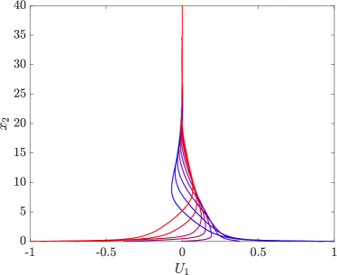
(a)

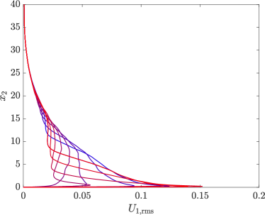
(b)

Figure 7: (a) Mean streamwise velocity profile and (b) streamwise r.m.s. velocity from $t\Omega=0$ (blue) to $t\Omega=\pi$ (red). The profiles shown are at $t\Omega=n\pi/8$, $n=0,1,...8$.

To construct the resolvent operator, we first choose the spatial scales for the homogeneous directions. Using the DNS data, we calculate the streamwise energy spectrum at $x_{2}=1.43$ and $t\Omega=2.65$, the wall-normal location and phase of the peak $U_{1,rms}$. The most energetic streamwise and spanwise scales at that location are $k_{1}=0.67$ and $k_{3}=2.67$, which we choose as the streamwise and spanwise scales for the resolvent operator. To solve the discrete system, we use a Chebyshev grid in the wall-normal direction, with $N_{2}=70$, and a uniform temporal discretization over one period $T\Omega=2\pi$, with $N_{t}=1600$.

We choose the first-order derivative matrix in time $\mathsfbi D_{t}$ and the wall-normal spatial derivative matrices to be second-order-accurate centered finite difference matrices. We additionally choose $\mathsfbi D_{t}$ to be circulant to enforce periodicity in time. We compute the modes for the half-channel and enforce a no-slip and no-penetration boundary condition at the wall, and a free-slip and no-penetration boundary condition at the centreline. Because $\mathsfbi D_{t}$ is a finite difference matrix rather than a Fourier differentiation matrix, we must implement a filtering step, detailed in §2.2.5, to exclude the high temporal wavenumbers. To apply this filtering step, we must assume that the high-frequency waves are not physically significant for the turbulent Stokes boundary layer problem. We use a two-stage Daubechies-16 wavelet transform, which is a sparse unitary operator. We note that the Daubechies-16 operator is not a perfect band-pass filter, and the numerical filtering operation simply attenuates the high-frequency waves that produce spurious SVD modes instead of excluding them outright. Nevertheless, due to the high dimensionality of the problem, it remains advantageous to use sparse transforms. We choose to constrain the forcing and response modes to the scaling functions and their shifts, which roughly cover the first fourth of all temporal wavenumbers $k_{t}=0...,N_{t}/8$.

We compare the results obtained with the wavelet-based resolvent modes with the results from harmonic resolvent analysis (Padovan et al., 2020). The latter computes a Fourier-based resolvent analysis simultaneously for multiple temporal wavenumbers and includes the interactions between them as they are coupled by the temporally evolving mean profile. For the harmonic resolvent analysis, we use the same Chebyshev grid as in the wavelet-based method, with $N_{2}=70$. For the sake of comparing with the wavelet-based method and to account for the filtering step, we choose a frequency resolution of $N_{t}=1600/4=400$. We expect the two methods to produce similar singular values and modes. The singular values and modes would be equivalent in both cases if we use a Fourier differentiation operator for the wavelet-based method as in §3.1.

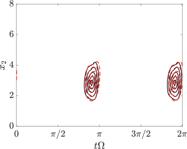
(a)

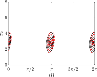
(b)

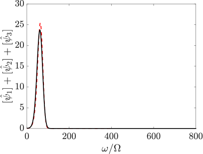
(c)

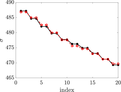
(d)

Figure 8: Magnitude contours ($10\%$, $25\%$, $50\%$, $75\%$ and $95\%$ of the maximum value) of (a) the wall-normal component of the principal resolvent forcing mode and (b) the streamwise component of the principal resolvent response mode for the turbulent Stokes boundary layer; (c) $x_{2}$–integrated Fourier spectrum in time for the principal response modes; (d) singular values from the SVD of the resolvent operators. Results from harmonic resolvent analysis are shown in red, and those from wavelet-based resolvent analysis in black.

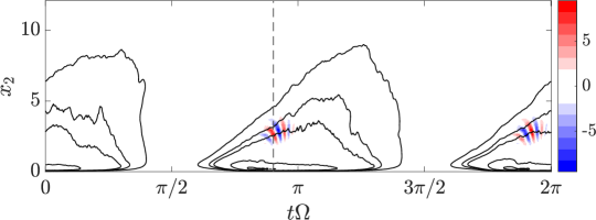
(a)

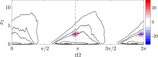
(b)

Figure 9: Real part of (a) $\breve{\phi}_{1}$, and (b) $\breve{\psi}_{1}$ for the turbulent Stokes boundary layer. The black contour lines are $U_{1,rms}$ with the levels indicating $30\%,50\%,75\%,95\%$ of its maximum value. The vertical dashed lines show the times of the amplitude peak for the input mode ($t\Omega=2.84$) and output mode ($t\Omega=3.03$).

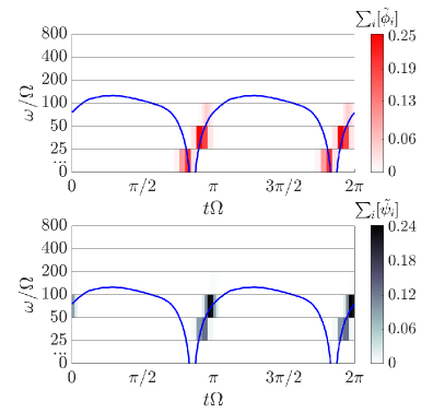
(a)

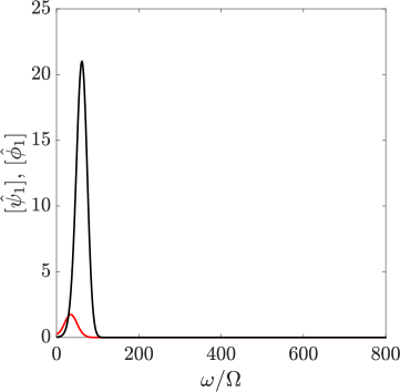
(b)

Figure 10: (a) Principal forcing (red, top panel) and response (black, bottom panel) modes in the time-frequency plane; the blue line indicates $U_{1}k_{1}/\Omega$ at $x_{2,\mathrm{avg}}^{\mathrm{resp.}}=x_{2,\mathrm{avg}}^{\mathrm{forc.}}\approx 0.071$; (b) $x_{2}$–integrated frequency content in the streamwise component of the forcing (red) and response (black) modes.

The modes obtained from harmonic resolvent analysis agree well with the those obtained from wavelet-based resolvent analysis. They occur at the same $x_{2}$ location, and time (figure 8(a)), and exhibit roughly the same frequency content (figure 8(b)). Moreover, the SVD of the wavelet-based and harmonic resolvent operators yield very similar singular values. The first twenty singular values are shown in figure 8(c). Despite Daubechies-16 wavelets being imperfect band-pass filters, filtering-out high-frequency waves using the sparse wavelet transform succeeds in producing resolvent modes that match the leading modes from harmonic resolvent analysis. Moreover, the windowed wavelet-based resolvent operator exhibits significant sparsity and can be analyzed efficiently, despite the larger dimension of the system.

The principal input and output modes corresponding to the chosen spatial scales and boundary conditions in time are shown in figure 9(a). We observe that the principal input and output modes are synchronised with the peaks in $U_{1,rms}$. The migration of the energy peak towards the centreline occurs at a similar rate for the resolvent modes as for the DNS results. This suggests that the energy amplification in the Stokes boundary layer can partially be explained by the optimal linear mechanism, similarly to the turbulent channel flow (Jiménez, 2013).

We also observe that the principal input mode precedes the principal output mode in time, with the peak of the former occurring $\Delta t\Omega\approx 0.19$ before the peak of the latter. Wavelet-based resolvent analysis is able to capture the natural response time between forcing and response terms under the dynamics of the linearised Navier-Stokes. This time delay is also in line with a physical interpretation of the modes in which the input modes cause the output modes and must thus occur earlier. The extent to which this captures important causal mechanisms within the full nonlinear system is yet to be determined. In future works, it would be interesting to project flow fields onto these time-separated resolvent forcing and response modes to test whether better correlations can be obtained between them in the transformed bases.

Additionally, we notice that the only nonzero wavelet coefficients of both the principal forcing and response modes are those corresponding the bottom fourth of the set of resolved frequencies i.e. the lowest four bands in the scalograms shown in figures 10(a). This validates the windowing step described above. We also see in figure 10(a) that the frequency content of the principal modes varies with time. The principle forcing mode is initially composed of lower-frequency waves, whose frequencies are centered in a band $[0,25\Omega]$; these waves are gradually shifted up to frequencies centered in $[25\Omega,50\Omega]$. Likewise, the waves composing the principle response mode, initially at frequencies centered in $[25\Omega,50\Omega]$ are also shifted up to higher frequencies. We propose that this frequency shift is due to the time-varying mean streamwise velocity $U_{1}$, which acts as a convection velocity and accelerates the resolvent forcing and response waves. We define the average location of the streamwise modes as

$$x^{\mathrm{resp.}}_{2,\mathrm{avg}}:=\frac{\int_{0}^{T}\int_{0}^{1}x_{2}|\breve{\psi}_{1}|^{2}dx_{2}dt}{\int_{0}^{T}\int_{0}^{1}|\breve{\psi}_{1}|^{2}dx_{2}dt},$$ (33)

and

$$x^{\mathrm{forc.}}_{2,\mathrm{avg}}:=\frac{\int_{0}^{T}\int_{0}^{1}x_{2}|\breve{\phi}_{1}|^{2}dx_{2}dt}{\int_{0}^{T}\int_{0}^{1}|\breve{\phi}_{1}|^{2}dx_{2}dt},$$ (34)

and plot the frequency shift due to the mean convection $U_{1}k_{1}/\Omega$ at the average mode locations in figure 10(a). We observe a good correlation between the shift in the frequency content of the forcing and response modes and the change in the mean velocity.

We can also use the changing mean velocity profile to explain the difference in the frequency content between the forcing and response modes. We propose that this difference in frequency content is due to the different peaking times of the forcing and response modes. Since the modes occur at difference phases of the oscillating mean profile, they will be convected at different velocities. To verify this, we first Fourier-transform $\boldsymbol{\breve{\phi}}$ and $\boldsymbol{\breve{\psi}}$ in time to extract their frequency content with better precision, and observe in figure 10(b) that the average frequency shift between the forcing and response modes is

$$\Delta\omega:=\frac{\int_{0}^{\Omega Nt/2}\omega[\hat{\psi}_{1}]d\omega}{\int_{0}^{\Omega Nt/2}[\hat{\psi}_{1}]d\omega}-\frac{\int_{0}^{\Omega Nt/2}\omega[\hat{\phi}_{1}]d\omega}{\int_{0}^{\Omega Nt/2}[\hat{\phi}_{1}]d\omega}\approx 26\;\Omega.$$ (35)

We then define the average temporal location of the modes as

$$t^{\mathrm{resp.}}_{\mathrm{avg}}:=\frac{\int_{0}^{T}t[\breve{\psi}_{1}]dt}{\int_{0}^{T}[\breve{\psi}_{1}]dt},$$ (36)

and

$$t^{\mathrm{forc.}}_{\mathrm{avg}}:=\frac{\int_{0}^{T}t[\breve{\phi}_{1}]dt}{\int_{0}^{T}\int_{0}^{1}[\breve{\phi}_{1}]dt}.$$ (37)

Assuming that both the optimal forcing and response prefer the same natural frequency $\omega_{0}$ with a corresponding streamwise wave speed $c_{0}=\omega_{0}/k_{1}$, we estimate the shift with

$$\left(|U(x^{\mathrm{resp.}}_{2,\mathrm{avg}},t^{\mathrm{resp.}}_{\mathrm{avg}})|-|U(x^{\mathrm{forc.}}_{2,\mathrm{avg}},t^{\mathrm{forc.}}_{\mathrm{avg}}|)\right)k_{1}/\Omega\approx 27,$$ (38)

which roughly matches the observed shift. We repeat this analysis for different spatial parameters $(k_{1},k_{3})=(1.33,2.67)$, though the plots are not shown. For these lengthscales, the expected frequency shift is found to be $\Delta\omega/\Omega\approx 14.6$ using (38), roughly matching the measured mean frequency shift of $\Delta\omega/\Omega\approx 13.4$ computed using a Fourier transform of the response and forcing modes. Wavelet-based resolvent analysis for this nonstationary flow thus reveals how a time-varying mean profile affects the linear amplification of perturbations. The mean velocity profile not only determines the spatial structure of the modes like in §3.1, but also their transient behaviour, and in this case, acts as a convection velocity that modulates their frequency content and wave speeds.

4.2 Channel flow with sudden lateral pressure gradient

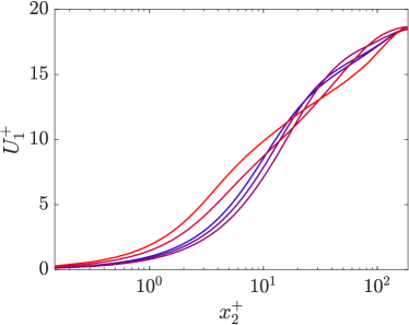
(a)

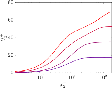
(b)

Figure 11: Mean (a) streamwise and (b) spanwise velocity profile from $t=0$ (blue) to $t=2.34$ (red). The times shown are $t=0,\,0.58,\,1.17,\,1.76,\,2.34$. Data taken from Lozano-Durán et al. (2021). Time $t$ is nondimensionalised with $u_{\tau,0}/\delta$

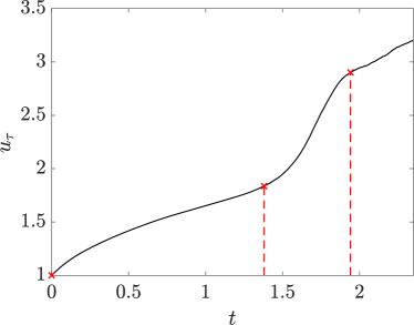
(a)

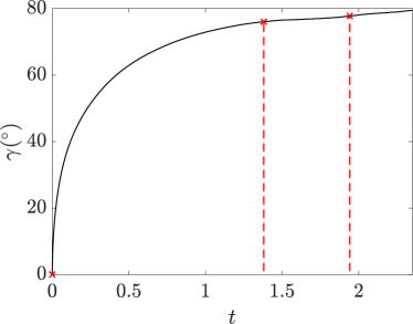
(b)

Figure 12: (a) Friction velocity $u_{\tau}$ and (b) wall-shear stress angle $\gamma=\tan^{-1}(\tau_{3}/\tau_{1})$ as a function of time. Data taken from Lozano-Durán et al. (2021). The vertical dashed lines are at $t=0,1.38,1.94$, and correspond to the choice of $\lambda_{1}^{+}$ and $\lambda_{3}^{+}$ for the modes plotted in figure 13

Finally, we study a fully-developed turbulent channel flow at $\Rey_{\tau}=186$ that is subjected to a sudden lateral pressure gradient $dP/dx_{3}=\Pi dP/dx_{1}$ at $t=0$ with $\Pi=30$ (Moin et al., 1990; Lozano-Durán et al., 2021). This flow, commonly referred to as a three-dimensional (3D) channel flow, has an initial transient period dominated by 3D non-equilibrium effects. Eventually, the flow will reach a new statistically steady state with the mean flow in the $(dP/dx_{1},dP/dx_{3})$ direction parallel to the wall. In the transient period, the tangential Reynolds stress initially decreases before increasing linearly, with depletion and increase rate that scales as $\Pi x_{2}/\delta$ (Lozano-Durán et al., 2021).

The mean flow profiles are obtained from Lozano-Durán et al. (2021) and have nonzero streamwise and spanwise components $U_{1}$ and $U_{3}$ (figure 11) as well as nonzero wall-normal gradients of streamwise and spanwise components $\mathsfbi{dU}_{1,2}$ and $\mathsfbi{dU}_{3,2}$. In this section, we nondimensionalise velocity by initial friction velocity $u^{*}_{\tau,0}$, lengths by the channel half-height $\delta^{*}$, and time by $\delta^{*}/u^{*}_{\tau,0}$. The Reynolds number for this problem is $\Rey=\Rey_{\tau,0}:=u^{*}_{\tau,0}\delta^{*}/\nu$. The time domain of the simulation is $T=2.34$. To construct the discrete resolvent operator, we use a Chebyshev grid of size $N_{2}=65$ in the $x_{2}-$ direction extending from $x_{2}=0$ to $x_{2}=1$. For the spatial derivatives in the $x_{2}-$ direction, we choose second-order accurate finite difference matrices. We enforce a no-slip and no-penetration boundary condition at the wall and a free-slip and no-penetration condition at the centreline. The boundary condition for the temporal finite difference operator $\mathsfbi D_{t}$ is chosen to enforce a Neumann-type condition, $\partial_{t}(\cdot)|_{t=0}=\partial_{t}(\cdot)|_{t=T}=0$. To reduce the impact of the boundary condition on the modes at $t=0$ we extend $U_{1}$ and $U_{3}$ to the time interval $t\in[-0.58,2.34]$ and assume $U_{i}(t\leq 0,y)=U_{i}(t=0,y)$ and $dP/dx_{3}(t<0)=0$. When the modes are plotted, we only show the original time domain $t\in[0,2.34]$ and exclude the contribution from negative times. We use a temporal resolution of $N_{t}=1000$ for the extended time frame. In this case, we note that we do not obtain spurious modes due to the distortion of high frequency waves, and that filtering-out those waves as in §4.1 has little effect on the results.

Regarding the spatial scales for the homogeneous directions, we choose them to capture near-wall streaks at three different times: $t=0$, $1.3$ and $1.94$. We thus tune them to represent the aspect ratio characteristic of near wall streaks, i.e. $\lambda_{1}^{+}\approx 10\lambda_{3}^{+}$ for a mean flow with a dominant streamwise component, and $\lambda_{3}^{+}\approx 10\lambda_{1}^{+}$ for a mean flow with a dominant spanwise component. Here, $(\cdot)^{+}$ indicates the wall scaling with $\Rey_{\tau,0}$, before the lateral pressure gradient is applied. To capture near-wall streaks at $t=0$, we choose $(\lambda_{1}^{+},\,\lambda_{3}^{+})=(1000,\,100)$ as in §3.1, which corresponds to the spatial scales preferred by the near-wall streaks at $\Rey_{\tau}=186$ prior to the lateral pressure gradient. Under the shear conditions at $t=1.3,\;1.94$, we must take into account the stronger mean shear in the spanwise direction (Lozano-Durán et al., 2021) by multiplying the by a factor of $\Rey_{\tau}(t)/\Rey_{\tau,0}=u^{*}_{\tau}(t)/u^{*}_{\tau,0}=u_{\tau}$, plotted in figure 12(a). We also take into account the new orientation of the streaks by applying a rotation by the wall-shear stress angle $\gamma(t)=\tan^{-1}(\tau_{3}/\tau_{1})$, where $\tau_{i}$ is the instantaneous wall-shear stress in the $x_{i}$ direction (see figure 12(b)). We thus obtain spatial parameters $(\lambda_{1}^{+},\,\lambda_{3}^{+})=(189,,1890)$ corresponding to $t=1.3$, and $(\lambda_{1}^{+},\,\lambda_{3}^{+})=(297,\,2970)$ corresponding to $t=1.94$.

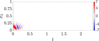
(a)

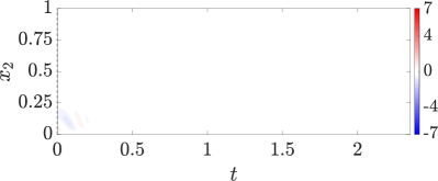
(b)

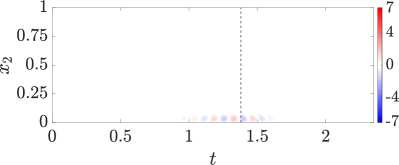
(c)

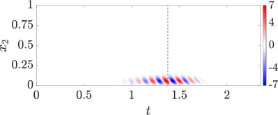
(d)

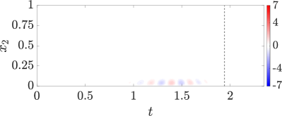
(e)

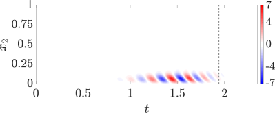
(f)

Figure 13: Real part of $\breve{\psi}_{1}$ (left) and $\breve{\psi}_{3}$ (right) for the turbulent channel subject to a spanwise pressure gradient. The chosen spatial scales are (a, b) $\lambda_{1}^{+}=1000$, $\lambda_{3}^{+}=100$, (c, d) $\lambda_{1}^{+}=189$, $\lambda_{3}^{+}=1890$, and (e, f) $\lambda_{1}^{+}=297$, $\lambda_{3}^{+}=2970$. The vertical dashed lines mark (a, b) $t=0$, (c, d) $t=1.38$, and (e, f) $t=1.94$.

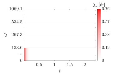
(a)

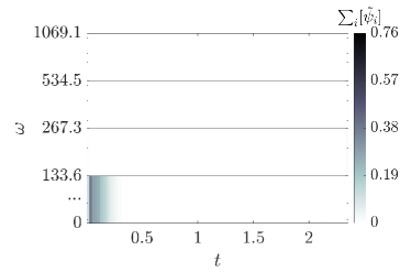
(b)

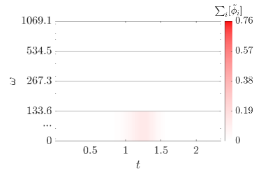
(c)

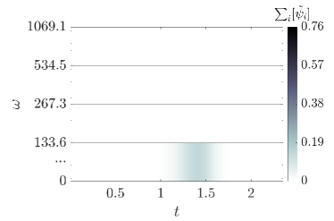
(d)

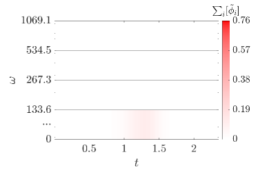
(e)

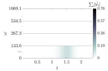
(f)

Figure 14: Principal forcing (left) response (right) modes in the frequency-time plane for the turbulent channel subject to a spanwise pressure gradient, for (a, b) $\lambda_{1}^{+}=1000$, $\lambda_{3}^{+}=100$, (c, d) $\lambda_{1}^{+}=189$, $\lambda_{3}^{+}=1890$, and (e, f) $\lambda_{1}^{+}=297$, $\lambda_{3}^{+}=2970$.

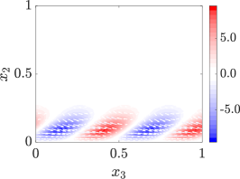
(a)

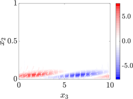
(b)

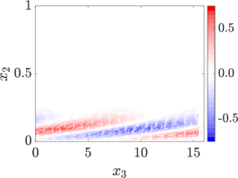
(c)

Figure 15: Principal response mode in the $x_{2}-x_{3}$ plane at (a) $t=0$, (b) $t=1.38$, and (c) $t=1.94$, rotated by $-\gamma$. The contours represent the streamwise component; the arrows represent the velocity field in the wall-parallel plane and are colored according to $\sqrt{|\psi_{2}|^{2}+|\psi_{3}|^{2}}\mathrm{sgn}(\psi_{3})$.

The resolvent modes for these scales are shown in figure 13(a,b). The magnitude of the modes in frequency-time space is also plotted in figure 14(a). The resolvent modes are temporally centered around $t=0$ and exhibit a predominant streamwise component. The modes are located in a region $x_{2}<0.25$, which corresponds to $x_{2}^{+}<45$, i.e., the buffer region. Thus, at $t=0$, the modes capture the highly energetic near-wall streaks. The subsequent temporal decay of these modes can be explained by the changing flow conditions, notably the growth of the spanwise wall-shear stress $\tau_{3}$, and consequently $u_{\tau}$ (see Figure 12). Under these conditions, the spatial scales preferred by the near-wall streaks stretch as $u_{\tau}$ increases and the wall-shear stress tensor rotates toward the $x_{3}$ direction.

The response mode for the second pair of spatial scales, $(\lambda_{1}^{+},\lambda_{3}^{+})=(189,1890)$, tuned to conditions at $t=1.38$, are plotted in 13(c,d). The frequency-time map of the modes is shown in figure 14(b). Similar to the first case, the modes are centered around $t=1.38$, indicating that the wavelet-based resolvent analysis is able to identify the nonequilibrium effects of the non-stationary flow. We note that the spanwise component of the response mode is much more dominant than the streamwise component, which reflects the new wall-shear angle $\gamma=75.7^{\circ}$. Finally, for the third case, $(\lambda_{1}^{+},\lambda_{3}^{+})=(297,2970)$, tuned to conditions at $t=1.94$, we observe that the modes (figure 13(e,f) and figure 14(c)) are not centered around the target time. We speculate that this is due to the temporal boundary condition at $t=2.34$. As the flow is not at a statistically-steady state at this time, a Neumann boundary condition may not be the most suitable boundary condition. The modes cannot grow beyond the boundary due to the boundary condition and are artificially damped near the end of the temporal domain.

We plot the principal response mode in the physical domain for the three target lengthscale pairs in figure 15, after applying a rotation of $-\gamma$ about the $x_{2}$–axis. The modes resemble each other qualitatively, and capture elongated near-wall streaks in the direction of the rotated flow. The response mode for $(\lambda_{1}^{+},\lambda_{3}^{+})=(297,2970)$ (figure 15(b)) is concentrated closer to the wall than for $(\lambda_{1}^{+},\lambda_{3}^{+})=(1000,100)$ (figure 15(a)), which indicates that the region of high-sensitivity to forcing moves closer to the wall as $Re_{\tau}$ increases. This is in line with the behaviour of near-wall turbulence: for higher $Re_{\tau}$, the buffer and logarithmic layers, which contain the bulk of turbulent energy in channel flow, are closer to the wall. Moreover, the length and spanwise spacing of the streaks increases with wall shear stress, as expected.

5 Conclusion

This work expands the resolvent analysis framework to non-stationary flow problems. The resolvent operator is traditionally constructed for flow quantities that are Fourier-transformed in the homogeneous spatial directions and in time. Such a resolvent operator cannot be used to study time-localised nonlinear forcing or a time-varying mean flow. Instead, we construct a wavelet-based resolvent operator, applying a wavelet transform in time while keeping the Fourier transform for the homogeneous spatial directions.

This resolvent operator, provided we use an orthonormal wavelet basis, is equivalent to the Fourier-based resolvent analysis for statistically stationary flows. Even in such cases, wavelet-based resolvent analysis can be modified through windowing in order to explore the effects of transient forcing localised to time scales of interest, such as those characterizing the logarithmic layer. In the case of transiently forced channel flow, the wavelet-based resolvent analysis with windowing reveals that the optimal response modes are transiently amplified rolls. The transient yet significant transient energy growth of these streaks is expected of non-normal systems. Moreover, the optimal forcing and response modes exhibit characteristics of the Orr mechanism, which supports the claim that this mechanism plays an important role in the linear amplification of velocity perturbations.

The wavelet-based resolvent analysis is notable in its ability to reflect the effects of a non-stationary mean flow. In the case of the turbulent Stokes boundary layer, the wavelet-based resolvent modes, which encode time, allow us to track the spatial and temporal location of the peak amplification alongside the varying mean flow. The resolvent modes reveal an increased sensitivity to forcing and perturbation amplification near the peaks of the streamwise root-mean-square velocity. This suggests that linear mechanisms may be an important source of energy amplification in this type of flow, as is believed for channel flow. We also observe that the input modes precede the output modes, opening the possibility to study causality in turbulent flows using resolvent analysis. Wavelet-based resolvent modes also encode frequency information. This ability sheds new light on the properties of linear amplification in the Stokes oscillating boundary layer: there exists an optimal forcing frequency to which the linearised flow is most sensitive, but the corresponding optimal response trajectory is shifted to higher frequencies by the decelerating mean flow. Wavelet-based resolvent analysis can thus be a useful tool for analyzing systems in which forcing and response prefer different frequencies.

Finally, for the 3D channel flow, the resolvent modes are able to identify the effect of the varying flow conditions, mainly the increasing shear velocity and rotating wall shear stress, on the principal resolvent modes. We compute the resolvent modes using the length scales preferred by near-wall streaks for flow conditions at three different times. The resulting resolvent response modes peak around the chosen times, with the exception of the time close to the end of the temporal domain. The predominant velocity component for the resolvent modes progressively shifts from the streamwise component to the spanwise one, mirroring the reorientation of the mean flow. Wavelet resolvent modes reflect time-varying mean flow conditions and help locate energetic near-wall streaks in space and time, and identify their preferred spatial scales. This can shed light on the flow conditions that amplify these coherent structures. Thus, the cases considered in this work showcase the versatility of the wavelet-based formulation in analyzing transient linear energy amplification in flows with either statistically stationary and non-stationary mean profiles.

Declaration of Interests

The authors report no conflict of interest.

References

- Abreu et al. (2020) Abreu, L. I., Cavalieri, A. V. G., Schlatter, P., Vinuesa, R. & Henningson, D. S. 2020 Spectral proper orthogonal decomposition and resolvent analysis of near-wall coherent structures in turbulent pipe flows. J. Fluid Mech. 900, A11.
- Adrian (2007) Adrian, R. J. 2007 Hairpin vortex organization in wall turbulence. Phys. Fluids 19 (4), 041301.
- Akhavan et al. (1991) Akhavan, R., Kamm, R. D. & Shapiro, A. H. 1991 An investigation of transition to turbulence in bounded oscillatory Stokes flows Part 1. Experiments. J. Fluid Mech. 225, 395–422.
- Arun et al. (2023) Arun, R., Bae, H. J. & McKeon, B. J. 2023 Towards real-time reconstruction of velocity fluctuations in turbulent channel flow. Phys. Rev. Fluids 8 (6), 064612.
- Bae et al. (2020) Bae, H. J., Dawson, S. T. M. & McKeon, B. J. 2020 Resolvent-based study of compressibility effects on supersonic turbulent boundary layers. J. Fluid Mech. 883, A29.
- Bae & Lee (2021) Bae, H. J. & Lee, M. 2021 Life cycle of streaks in the buffer layer of wall-bounded turbulence. Phys. Rev. Fluids 6 (6), 064603.
- Bae et al. (2018) Bae, H. J., Lozano-Durán, A., Bose, S. T. & Moin, P. 2018 Turbulence intensities in large-eddy simulation of wall-bounded flows. Phys. Rev. Fluids 3, 014610.
- Bae et al. (2019) Bae, H. J., Lozano-Durán, A., Bose, S. T. & Moin, P. 2019 Dynamic slip wall model for large-eddy simulation. J. Fluid Mech. 859, 400–432.
- Bae et al. (2021) Bae, H. J., Lozano-Durán, A. & McKeon, B. J. 2021 Nonlinear mechanism of the self-sustaining process in the buffer and logarithmic layer of wall-bounded flows. J. Fluid Mech. 914, A3.
- Bakewell & Lumley (1967) Bakewell, H. P. Jr. & Lumley, J. L. 1967 Viscous sublayer and adjacent wall region in turbulent pipe flow. Phys. Fluids 10 (9), 1880–1889.
- Ballouz et al. (2023a) Ballouz, E., Dawson, S. T. M. & Bae, H. J. 2023a Transient growth of wavelet-based resolvent modes in the buffer layer of wall-bounded turbulence. arXiv preprint arXiv:2312.15465 .
- Ballouz et al. (2023b) Ballouz, E., Lopez-Doriga, B., Dawson, S. T. M. & Bae, H. J. 2023b Wavelet-based resolvent analysis for statistically-stationary and temporally-evolving flows. In AIAA SCITECH 2023 Forum, p. 0676.
- Barthel & Sapsis (2023) Barthel, B. & Sapsis, T. 2023 Harnessing instability mechanisms in airfoil flow for data-driven forecasting of extreme events. AIAA 61 (11), 4879–4896.
- Beneddine et al. (2017) Beneddine, S., Yegavian, R., Sipp, D. & Leclaire, B. 2017 Unsteady flow dynamics reconstruction from mean flow and point sensors: an experimental study. J. Fluid Mech. 824, 174–201.
- Berkooz et al. (1993) Berkooz, G., Holmes, P. & Lumley, J. L. 1993 The proper orthogonal decomposition in the analysis of turbulent flows. Annu. Rev. Fluid Mech. 25 (1), 539–575.
- Blackwelder & Eckelmann (1979) Blackwelder, R. F. & Eckelmann, H. 1979 Streamwise vortices associated with the bursting phenomenon. J. Fluid Mech. 94 (3), 577–594.
- Blondeaux & Vittori (1994) Blondeaux, P. & Vittori, G 1994 Wall imperfections as a triggering mechanism for Stokes-layer transition. J. Fluid Mech. 264, 107–135.
- Borée (2003) Borée, J 2003 Extended proper orthogonal decomposition: a tool to analyse correlated events in turbulent flows. Exp. Fluids 35 (2), 188–192.
- Butler & Farrell (1993) Butler, K. M. & Farrell, B. F. 1993 Optimal perturbations and streak spacing in wall-bounded turbulent shear flow. Phys. Fluids A 5 (3), 774–777.
- Carstensen et al. (2010) Carstensen, S., Sumer, B. M. & Fredsøe, J. 2010 Coherent structures in wave boundary layers. Part 1. Oscillatory motion. J. Fluid Mech. 646, 169–206.
- Chernyshenko & Baig (2005) Chernyshenko, S. I. & Baig, M. F. 2005 The mechanism of streak formation in near-wall turbulence. J. Fluid Mech. 544, 99–131.
- Costamagna et al. (2003) Costamagna, P., Vittori, G. & Blondeaux, P. 2003 Coherent structures in oscillatory boundary layers. J. Fluid Mech. 474, 1–33.
- Del Alamo & Jimenez (2006) Del Alamo, J. C. & Jimenez, J. 2006 Linear energy amplification in turbulent channels. J. Fluid Mech. 559, 205–213.
- Drineas & Mahoney (2016) Drineas, P. & Mahoney, M. W. 2016 RandNLA: randomized numerical linear algebra. Commun. ACM 59 (6), 80–90.
- Encinar & Jiménez (2020) Encinar, M. P. & Jiménez, J. 2020 Momentum transfer by linearised eddies in turbulent channel flows. J. Fluid Mech. 895, A23.
- Farrell et al. (2017) Farrell, B. F., Gayme, D. F. & Ioannou, P. J. 2017 A statistical state dynamics approach to wall turbulence. Phil. Trans. R. Soc. Lond. A 375 (2089), 20160081.
- Farrell & Ioannou (1998) Farrell, B. F. & Ioannou, P. J. 1998 Perturbation structure and spectra in turbulent channel flow. Theor. Comput. Fluid Dyn. 11 (3), 237–250.
- Floryan & Graham (2021) Floryan, D. & Graham, M. D. 2021 Discovering multiscale and self-similar structure with data-driven wavelets. Proc. Natl. Acad. Sci. USA 118 (1), e2021299118.
- Gómez et al. (2016) Gómez, F., Blackburn, H. M., Rudman, F., Sharma, A. S. & McKeon, B. J. 2016 A reduced-order model of three-dimensional unsteady flow in a cavity based on the resolvent operator. J. Fluid Mech. 798, R2.
- Halko et al. (2011) Halko, N., Martinsson, P.-G. & Tropp, J. A. 2011 Finding structure with randomness: Probabilistic algorithms for constructing approximate matrix decompositions. SIAM Rev. 53 (2), 217–288.
- Hamilton et al. (1995) Hamilton, J. M., Kim, J. & Waleffe, F. 1995 Regeneration mechanisms of near-wall turbulence structures. J. Fluid Mech. 287, 317–348.
- Hino et al. (1976) Hino, M., Sawamoto, M. & Takasu, S. 1976 Experiments on transition to turbulence in an oscillatory pipe flow. J. Fluid Mech. 75 (2), 193–207.
- Hoyas & Jiménez (2006) Hoyas, S. & Jiménez, J. 2006 Scaling of velocity fluctuations in turbulent channels up to . Phys. Fluids 18, 011702.
- Hoyas & Jiménez (2008) Hoyas, S. & Jiménez, J. 2008 Reynolds number effects on the Reynolds-stress budgets in turbulent channels. Phys. Fluids 20 (10), 101511.
- Hwang & Cossu (2010) Hwang, Y. & Cossu, C. 2010 Self-sustained process at large scales in turbulent channel flow. Phys. Rev. Lett. 105 (4), 044505.
- Illingworth et al. (2018) Illingworth, S. J., Monty, J. P. & Marusic, I. 2018 Estimating large-scale structures in wall turbulence using linear models. J. Fluid Mech. 842, 146–162.
- Jensen et al. (1989) Jensen, B. L., Sumer, B. M. & Fredsøe, J. 1989 Turbulent oscillatory boundary layers at high Reynolds numbers. J. Fluid Mech. 206, 265–297.
- Jeun et al. (2016) Jeun, J., Nichols, J. W. & Jovanović, M. R. 2016 Input-output analysis of high-speed axisymmetric isothermal jet noise. Phys. Fluids 28.4, 047101.
- Jiménez (2013) Jiménez, J. 2013 How linear is wall-bounded turbulence? Phys. Fluids 25, 110814.
- Jiménez (2015) Jiménez, J. 2015 Direct detection of linearized bursts in turbulence. Phys. Fluids 27 (6), 065102.
- Jiménez (2018) Jiménez, J. 2018 Coherent structures in wall-bounded turbulence. J. Fluid Mech. 842, P1.
- Jiménez & Moin (1991) Jiménez, J. & Moin, P. 1991 The minimal flow unit in near-wall turbulence. J. Fluid Mech. 225, 213–240.
- Jiménez & Pinelli (1999) Jiménez, J. & Pinelli, A. 1999 The autonomous cycle of near-wall turbulence. J. Fluid Mech. 389, 335–359.
- Johansson et al. (1987) Johansson, A. V., Her, J.-Y. & Haritonidis, J. H. 1987 On the generation of high-amplitude wall-pressure peaks in turbulent boundary layers and spots. J. Fluid Mech. 175, 119–142.
- Jovanovic (2004) Jovanovic, M. R 2004 Modeling, analysis, and control of spatially distributed systems. University of California at Santa Barbara, Dept. of Mechanical Engineering.
- Jovanović & Bamieh (2005) Jovanović, M. R. & Bamieh, B. 2005 Componentwise energy amplification in channel flows. J. Fluid Mech. 534, 145–183.
- Kim et al. (1971) Kim, H. T., Kline, S. J. & Reynolds, W. C. 1971 The production of turbulence near a smooth wall in a turbulent boundary layer. J. Fluid Mech. 50 (1), 133–160.
- Kim & Moin (1985) Kim, J. & Moin, P. 1985 Application of a fractional-step method to incompressible Navier-Stokes equations. J. Comp. Phys. 59, 308–323.
- Klebanoff et al. (1962) Klebanoff, P. S., Tidstrom, K. D. & Sargent, L. M. 1962 The three-dimensional nature of boundary-layer instability. J. Fluid Mech. 12 (1), 1–34.
- Kline et al. (1967) Kline, S. J., Reynolds, W. C., Schraub, F. A. & Runstadler, P. W. 1967 The structure of turbulent boundary layers. J. Fluid Mech. 30 (4), 741–773.
- Kojima et al. (2020) Kojima, Y., Yeh, C., Taira, K. & Kameda, M. 2020 Resolvent analysis on the origin of two-dimensional transonic buffet. J. Fluid Mech. 885, R1.
- Landahl (1975) Landahl, M. T 1975 Wave breakdown and turbulence. SIAM J. Appl. Math 28 (4), 735–756.
- Landahl (1980) Landahl, M. T. 1980 A note on an algebraic instability of inviscid parallel shear flows. J. Fluid Mech. 98 (2), 243–251.
- Lewalle (1993) Lewalle, J. 1993 Wavelet transforms of the Navier-Stokes equations and the generalized dimensions of turbulence. Appl. Sci. Res. 51 (1-2), 109–113.
- Lopez-Doriga et al. (2023) Lopez-Doriga, B., Ballouz, E., Bae, H. J. & Dawson, S. T. M. 2023 A sparsity-promoting resolvent analysis for the identification of spatiotemporally-localized amplification mechanisms. In AIAA SCITECH 2023 Forum, p. 0677.
- Lopez-Doriga et al. (2024) Lopez-Doriga, B., Ballouz, E., Bae, H. J. & Dawson, S. T. M. 2024 Sparse space-time resolvent analysis for statistically stationary and time-varying flows .
- Lozano-Durán & Bae (2019) Lozano-Durán, A. & Bae, H. J. 2019 Characteristic scales of Townsend’s wall-attached eddies. J. Fluid Mech. 868, 698.
- Lozano-Durán et al. (2021) Lozano-Durán, A., Constantinou, Navid C., Nikolaidis, M.-A. & Karp, M. 2021 Cause-and-effect of linear mechanisms sustaining wall turbulence. J. Fluid Mech. 914, A8.
- Lozano-Durán et al. (2021) Lozano-Durán, A., Giometto, M. G., Park, G. I. & Moin, P. 2021 Non-equlibrium three-dimensional boundary layers at moderate reynolds numbers. J. Fluid Mech. 883, A20.
- Lozano-Durán et al. (2018) Lozano-Durán, A., Hack, M. J. P. & Moin, P. 2018 Modeling boundary-layer transition in direct and large-eddy simulations using parabolized stability equations. Phys. Rev. Fluids 3, 023901.
- Luhar et al. (2014) Luhar, M., Sharma, A. S. & McKeon, B. J. 2014 Opposition control within the resolvent analysis framework. J. Fluid Mech. 749, 597–626.
- Lumley (1967) Lumley, J. L. 1967 The structure of inhomogeneous turbulent flows. Atmospheric turbulence and radio wave propagation pp. 166–178.
- Lumley (2007) Lumley, J. L. 2007 Stochastic tools in turbulence. Courier Corporation.
- Mallat (2001) Mallat, S. 2001 A Wavelet Tour of Signal Processing. Academic Press.
- Martini et al. (2020) Martini, E., Cavalieri, A. V. G., Jordan, P., Towne, A. & Lesshafft, L. 2020 Resolvent-based optimal estimation of transitional and turbulent flows. J. Fluid Mech. 900, A2.
- McKeon (2017) McKeon, B. J. 2017 The engine behind (wall) turbulence: perspectives on scale interactions. J. Fluid Mech. 817, P1.
- McKeon (2019) McKeon, B. J. 2019 Self-similar hierarchies and attached eddies. Phys. Rev. Fluids 4 (8), 082601.
- McKeon & Sharma (2010) McKeon, B. J. & Sharma, A. S. 2010 A critical-layer framework for turbulent pipe flow. J. Fluid Mech. 658, 336–382.
- Meneveau (1991) Meneveau, C. 1991 Analysis of turbulence in the orthonormal wavelet representation. J. Fluid Mech. 232, 469–520.
- Meyer (1992) Meyer, Y. 1992 Wavelets and Operators: Volume 1. Cambridge University Press.
- Mezić (2013) Mezić, I. 2013 Analysis of fluid flows via spectral properties of the Koopman operator. Annu. Rev. Fluid Mech. 45, 357–378.
- Moarref et al. (2013) Moarref, R., Sharma, A. S., Tropp, J. A. & McKeon, B. J. 2013 Model-based scaling of the streamwise energy density in high-Reynolds-number turbulent channels. J. Fluid Mech. 734, 275–316.
- Moin et al. (1990) Moin, P., Shih, T.-H., Driver, D. M. & Mansour, N. N. 1990 Direct numerical simulation of a three-dimensional turbulent boundary layer. Phys. Fluids 2 (10), 1846–1853.
- Musco & Musco (2015) Musco, C. & Musco, C. 2015 Randomized block krylov methods for stronger and faster approximate singular value decomposition. Adv. Neural Inf. Process Syst. 28, 1396–1404.
- Najmi (2012) Najmi, A.-H. 2012 Wavelets: A Concise Guide. The Johns Hopkins University Press.
- Orlandi (2000) Orlandi, P. 2000 Fluid flow phenomena: a numerical toolkit. Springer Science & Business Media.
- Orr (1907) Orr, W. M. 1907 The stability or instability of the steady motions of a perfect liquid and of a viscous liquid. Part I: A perfect liquid. Proc. R. Ir. Acad. A 27, 9–68.
- Ozdemir et al. (2014) Ozdemir, C. E., Hsu, T.-J. & Balachandar, S. 2014 Direct numerical simulations of transition and turbulence in smooth-walled Stokes boundary layer. Phys. Fluids 26 (4), 045108.
- Padovan et al. (2020) Padovan, A., Otto, S. E. & Rowley, C. W. 2020 Analysis of amplification mechanisms and cross-frequency interactions in nonlinear flows via the harmonic resolvent. J. Fluid Mech. 900, A14.
- Panton (2001) Panton, R. L. 2001 Overview of the self-sustaining mechanisms of wall turbulence. Prog. Aerosp. Sci. 37 (4), 341–383.
- Pickering et al. (2020) Pickering, E., Rigas, G., Nogueira, P. A. S., Cavalieri, A. V. G., Schmidt, O. T. & Colonius, T. 2020 Lift-up, Kelvin–Helmholtz and Orr mechanisms in turbulent jets. J. Fluid Mech. 896, A2.
- Pujals et al. (2009) Pujals, G., García-Villalba, M., Cossu, C. & Depardon, S. 2009 A note on optimal transient growth in turbulent channel flows. Phys. Fluids 21 (1), 015109.
- Ren et al. (2021) Ren, J., Mao, X. & Fu, S. 2021 Image-based flow decomposition using empirical wavelet transform. J. Fluid Mech. 906, A22.
- Ribeiro et al. (2020) Ribeiro, J. H. M., Yeh, C.-A. & Taira, K. 2020 Randomized resolvent analysis. Phys. Rev. Fluids 5 (3), 033902.
- Robinson (1991) Robinson, S. K. 1991 Coherent motions in the turbulent boundary layer. Annu. Rev. Fluid Mech. 23 (1), 601–639.
- Sarpkaya (1993) Sarpkaya, T. 1993 Coherent structures in oscillatory boundary layers. J. Fluid Mech. 253, 105–140.
- Schmid et al. (2002) Schmid, P. J., Henningson, D. S. & Jankowski, D. F. 2002 Stability and transition in shear flows. applied mathematical sciences, vol. 142. Appl. Mech. Rev. 55 (3), B57–B59.
- Schmidt et al. (2018) Schmidt, O. T., Towne, A., Rigas, G., Colonius, T. & Brès, G. A. 2018 Spectral analysis of jet turbulence. J. Fluid Mech. 855, 953–982.
- Schoppa & Hussain (2002) Schoppa, W. & Hussain, F. 2002 Coherent structure generation in near-wall turbulence. J. Fluid Mech. 453, 57–108.
- Simon & Zha (2000) Simon, H. D. & Zha, H. 2000 Low-rank matrix approximation using the Lanczos bidiagonalization process with applications. SIAM J. Sci. Comput. 21 (6), 2257–2274.
- Smith & Metzler (1983) Smith, C. R. & Metzler, S. P. 1983 The characteristics of low-speed streaks in the near-wall region of a turbulent boundary layer. J. Fluid Mech. 129, 27–54.
- Smits et al. (2011) Smits, A. J., McKeon, B. J. & Marusic, I. 2011 High–Reynolds number wall turbulence. Annu. Rev. Fluid Mech. 43, 353–375.
- Spalart & Baldwin (1989) Spalart, P. R. & Baldwin, B. S. 1989 Direct simulation of a turbulent oscillating boundary layer. In Turbulent shear flows 6, pp. 417–440. Springer.
- Tissot et al. (2021) Tissot, G., Cavalieri, A. V. G. & Mémin, E. 2021 Stochastic linear modes in a turbulent channel flow. J. Fluid Mech. 912, A51.
- Tissot et al. (2017) Tissot, G., Zhang, M., Lajús, F. C., Cavalieri, A. V. G. & Jordan, P. 2017 Sensitivity of wavepackets in jets to nonlinear effects: the role of the critical layer. J. Fluid Mech. 811, 95–137.
- Towne et al. (2020) Towne, A., Lozano-Durán, A. & Yang, X. I. A. 2020 Resolvent-based estimation of space–time flow statistics. J. Fluid Mech. 883, A17.
- Tropp et al. (2017) Tropp, J. A., Yurtsever, A., Udell, M. & Cevher, V. 2017 Practical sketching algorithms for low-rank matrix approximation. SIAM J. Matrix Anal. Appl. 38 (4), 1454–1485.
- Verzicco & Vittori (1996) Verzicco, R. & Vittori, G. 1996 Direct simulation of transition in Stokes boundary layers. Phys. Fluids 8 (6), 1341–1343.
- Vittori & Verzicco (1998) Vittori, G. & Verzicco, R. 1998 Direct simulation of transition in an oscillatory boundary layer. J. Fluid Mech. 371, 207–232.
- Von Kerczek & Davis (1974) Von Kerczek, C. & Davis, S. H. 1974 Linear stability theory of oscillatory Stokes layers. J. Fluid Mech. 62 (4), 753–773.
- Waleffe (1997) Waleffe, F. 1997 On a self-sustaining process in shear flows. Phys. Fluids 9 (4), 883–900.
- Wray (1990) Wray, A. A. 1990 Minimal-storage time advancement schemes for spectral methods. Tech. Rep.. NASA Ames Research Center.
- Yeh et al. (2020) Yeh, C.-A., Benton, S. I., Taira, K. & Garmann, D. J. 2020 Resolvent analysis of an airfoil laminar separation bubble at . Physical. Rev. Fluids 5 (8), 083906.
- Yeh & Taira (2019) Yeh, C.-A. & Taira, K. 2019 Resolvent-analysis-based design of airfoil separation control. J. Fluid Mech. 867, 572–610.