Extremes of generalized inversions and descents
on permutation groups
Abstract.
The classical inversion statistic on symmetric groups is the sum of all indicators for a random permutation and the pairs with . The descent statistic counts all with . The number of inversions can be generalized by restricting the indicators to pairs with and for some . Likewise, the number of descents can be generalized by counting all with . These generalized statistics can be further extended to the signed and even-signed permutation groups. The bandwidth index can be chosen in dependence of , and the magnitude of is significant for asymptotic considerations. It is known that each of these statistics is asymptotically normal for suitable choices of . In this paper we prove the bivariate asymptotic normality and determine the extreme value asymptotics of generalized inversions and descents.
Key words and phrases:
extreme values, CLT, permutation statistics, Coxeter group2010 Mathematics Subject Classification:
Primary: 60G70, 05A16; Secondary: 20F551. Introduction
The numbers of inversions and descents are two important quantities of permutations. For a permutation an inversion is a pair with but . A descent is an index with , i.e., descents correspond to adjacent inversions. We now equip the symmetric group with the discrete uniform probability measure induced by the point masses . In this context, we denote the random numbers of inversions and descents as and . These random variables can also be represented with help of i.i.d. standard uniform variables , namely,
| (1) | ||||
In (1), we have to sum the indicators over all pairs with . A class of generalized inversion statistics can be constructed by restricting the sum in (1) to pairs with , for some . Writing , we can state that
| (2) |
counts the so-called -inversions. The term generalized inversions is an umbrella term for all -inversions. By choosing or it is seen that this class includes common inversions and descents. Moreover, -descents or generalized descents are given by
| (3) |
Generalized inversions were first introduced by de Mari & Shayman [5] to solve a problem in algebraic geometry. The first stochastic considerations for the random variables are due to Bona [2] and Pike [10], who computed the mean and variance and proved a central limit theorem (CLT).
Symmetric groups belong to the class of finite irreducible Coxeter groups, which have been classified by [4]. The concept of inversions and descents can be transferred to these groups, see [1, Section 1.4]. Two other important subfamilies of the finite irreducible Coxeter groups are the signed permutation groups and the even-signed permutation groups . The group consists of all maps for which is a permutation. Such a map is called a signed permutation. The groups are the subgroups of containing all signed permutations with an even number of negative signs. The random number of inversions on these groups can be represented with help of i.i.d. variables as follows:
| (4a) | ||||
| (4b) | ||||
We refer to the three families and as the classical Weyl groups. Recently, Meier & Stump [9] extended the concept of generalized inversions and descents to the groups and , again proving a CLT.
The investigation of extreme value asymptotics for common inversions and descents was initiated in [7, 6], so we aim to extend this knowledge to generalized inversions. We aim to prove Gumbel attraction for both the stand-alone statistics and the joint statistic . Here, and can be either fixed or dependent on . We will investigate the impact of the choice of for these results.
This paper is structured as follows. Section 2 gives basic properties on generalized inversions and descents, and introduces Hájek projections that are used as independent sum approximations. Section 3 deduces the bivariate CLT and the extreme value theorems for generalized inversions and descents. Section 4 gives the proofs of two auxiliary lemmas determining the choices of for which the Hájek projection serves as a working approximation. We use typical Landau notation for positive sequences as follows:
-
•
means that .
-
•
means that . This is also written as or .
-
•
means that and have the same order of magnitude, i.e., both and hold.
-
•
means that are sequences of random variables with .
2. Basic definitions
Definition 2.1.
Let be a symmetric group and let . For , -inversions are all pairs in with . In this sense, common descents equal -inversions, and common inversions equal -inversions. Moreover, -descents are all numbers with . We write for the random number of -inversions and for the number of -descents. Probabilistic representations are given in (2), (3). 111In the literature, there are different terminologies, e.g., in [2, 10], -inversions are called -descents. However, we use the terms and notation provided in [9].
Remark 2.2.
Obviously, every number can appear in at most -inversions. This bound is redundant if . In fact, it is an important case distinction whether or , e.g., when calculating the mean and variance of and . In the case of we can split into the regions
For each all larger indices and all smaller indices allow to form -inversions. For any there are less than indices available in one direction. If , then smaller indices are available for -inversions, which is less than numbers. If is large, then there are only larger indices available.
On the contrary, if then and the above partition into three regions is now written as
Now, if then there are only smaller indices and larger indices available to form -inversions.
The mean and variance of have been extensively computed by Pike [10]. It is easy to verify that the special cases and are consistent with [8, Corollaries 3.2 and 4.2]. The proof of [10, Theorem 1] is reviewed in [9, Theorem A.1], where the variance of -descents is provided as well.
Theorem 2.3 (see [10], Theorem 1 and [9], Theorem A.1).
For all it holds that
Moreover, if then
If then
and .
Meier & Stump [9] introduced an extension of generalized inversions and descents from symmetric groups to the other classical Weyl groups and . This extension is based on the root poset of a classical Weyl group. We refer to [9, Section 2] for the details. On the symmetric group , the ordered pairs of indices correspond to the positive roots , where are unit vectors in , and the height of within the root poset is .
On the signed permutation group we also have to consider the positive roots and for . The heights of these additional roots are and . The root corresponds to the indicator appearing in (4a), while corresponds to . See [9, Example 2.2] for an illustration of the root poset of . On the even-signed permutation group the roots are disregarded, and has height .
Definition 2.4.
For any classical Weyl group, -inversions are determined by roots of height at most , and -descents are determined by roots of height exactly , see [9, Definition 2.4]. For symmetric groups, this coincides with Definition 2.7. In addition to , we introduce
Then, on the signed and even-signed permutation groups, and can be expressed as follows:
| (5a) | ||||
| (5b) | ||||
| (5c) | ||||
| (5d) | ||||
Remark 2.5.
The largest possible choice of equals the total height of the root poset, namely, , where denotes the largest degree of the underlying classical Weyl group. In particular, for for and for . To precisely compute the variance of and on the groups and one needs to distinguish eight cases, as seen in [9, Theorems A.4 and A.13]. However, many of these cases give the same asymptotic quantification, which can be stated as follows:
Lemma 2.6 (cf. [9], Theorems A.4 and A.13).
For the generalized inversions and descents on both the groups and it holds that
An evident issue seen in (2), (5a), and (5b) is the mutual dependence of the indicators and . Therefore, we aim to approximate with a sum of independent variables. Hájek projections are a common tool for this.
Definition 2.7.
Let be independent random variables, and let be another random variable. Then, the Hájek projection of with respect to is given by
As every is a measurable function only in , the Hájek projection is a sum of independent random variables. If is a sequence of random variables with each depending on , then the Hájek projections should give a sufficiently accurate approximation to . To ensure this, the following criterion is useful.
Theorem 2.8 (cf. [11], Theorem 11.2).
Consider a sequence of random variables and their associated Hájek projections . If as then
3. Asymptotic results
Asymptotic normality
For the univariate statistics and , the asymptotic normality has been proven in [9]. For the joint statistic , the simplest case is when remains fixed. Then, both and are -dependent and it is not necessary to apply the Hájek approximation. From the CLT for -dependent random vectors, it follows that:
Theorem 3.1.
For any two fixed numbers the joint distribution satisfies the CLT.
An even stronger statement than the CLT is the uniform Gaussian approximation over all hyperrectangles for -dependent random vectors given in [3, Theorem 2]. It also applies for random vectors with a sparse dependency graph. Let be a triangular array of (w.l.o.g., centered) -dimensional random vectors and let
Let be the system of all -dimensional hyperrectangles, including infinite bounds, i.e., Let
In particular, is an upper bound for
which is relevant for the CLT, and for
which is relevant for the asymptotics of extreme values. Now, let be a dependency graph for which consists of all edges for which and are dependent. Let be the maximum degree of and let be the maximum degree of the 2-reachability graph of . If the graphs are not too dense as then can be bounded as follows:
Theorem 3.2 (cf. [3], Theorem 2).
Let be as above. Under some conditions which are satisfied by bounded variables, it holds that
In particular, if is -dependent for some global constant then .
This theorem was stated by Chang et al. for high dimensions, but it also works with fixed by artificially repeating the components of a random vector in fixed dimension.
From now, we consider the univariate statistics and the joint statistic for two sequences with . Both and are based on a sequence of classical Weyl groups where each is one of or .
If grows as , then there exists no constant for which all are -dependent. However, the dependency structure of is still sparse. Recall that and are constructed from i.i.d. random variables . According to (3), (5c), (5d), we can represent as a sum of indicator variables, each of which depends on at most three others. Therefore, the first-order and second-order maximum degrees are bounded in the way of and . In conclusion, there are no issues with applying Theorem 3.2 if grows.
If grows as well, then the maximum degrees of are bounded in the way of and . Moreover, we have to take into account that by (2), (5a), (5b), is based on summands, so we have to replace with in Theorem 3.2. Therefore, Theorem 3.2 gives an bound of if and only if . For any faster growth rate of the dependency structure of is too complex to apply Theorem 3.2. In that case, we have to replace with the Hájek projection . The growth rate of determines whether the condition in Theorem 2.8 is fulfilled or not. To classify the validity of this condition, we distinguish the short case and the long case .
Lemma 3.3.
Given the short case, we have for symmetric groups that
and we have for the groups and . So, if then .
Lemma 3.4.
Given the long case, holds on symmetric groups if and only if . On the other classical Weyl groups, holds if and only if or .
From Theorem 3.2 and Slutsky’s lemma, we can conclude:
Extreme values of the univariate statistics and
We now postulate the univariate and bivariate extreme value limit theorems (EVLTs) for and with the help of the methods used in [6]. The proof of [6, Theorem 4.1] consists of two parts. The first part is to show the Gumbel attraction of the statistic that replaces with . This is done by an application of [3, Theorem 2], providing Gaussian approximation for -dependent random vectors. The second part is to show that the error resulting from this replacement vanishes in probability. Recall that by use of
the maximum of i.i.d. variables is attracted to the Gumbel distribution, that is, :
Likewise, the two-dimensional standard normal distribution is attracted to the two-dimensional Gumbel distribution with independent marginals. Taking and writing ”” for component-wise multiplication, we get that for i.i.d. bivariate standard normal and :
Since the random numbers of generalized inversions and descents are discrete distributions, we are interested in the extremes of a triangular array where for each the block consists of i.i.d. samples taken from the -th symmetric group . Each of the following EVLTs imposes an upper bound on the number of samples .
For a univariate triangular array consisting of generalized descents, it is not necessary to use the Hájek projection. It has already been argued in [6, Remark 4.2] that a subexponential bound of can be obtained if the Hájek projection is not needed. So, in the univariate EVLT for generalized descents, we can use the bound of stated in [6, Remark 4.2]:
Theorem 3.6.
Let be a row-wise i.i.d. triangular array with for any sequence with and let . Let and let If then
A similar statement applies to if grows slow enough to permit the application of Theorem 3.2.
Theorem 3.7.
Let be a row-wise i.i.d. triangular array with , where . Let be given in analogy to Theorem 3.6. If then
Proof.
According to the above considerations, the maximum degrees in the dependency graph of the representations (2), (5a), and (5b) are bounded in the way of and . Since these representations are based on summands, we need to replace with when applying Theorem 3.2. An application of Theorem 3.2 with i.i.d. iterations of yields
where is the maximum of i.i.d. copies of the standard normal distribution. The claim follows. ∎
For any other growth rate of we can state an EVLT only for the cases covered by Lemmas 3.3 and 3.4, and due to the use of Hájek’s projection, we can only impose a strongly reduced asymptotic bound for .
Theorem 3.8.
Proof.
The conditions on ensure that but the rate of convergence determines the bound for by means of [6, Eq. (9), (10)]. We compute this rate for symmetric groups, since the same conclusions can be obtained on the other classical Weyl groups. In the short case, we have
Apparently, always dominates . In conclusion,
giving the condition of according to the arguments in the proof of [6, Theorem 4.1]. The remaining steps of the proof are the same.
In the long case, we write and note that
Therefore,
giving the requirement of
Again, the proof now follows the same steps as in [6, Theorem 4.1]. ∎
Remark 3.9.
This result is only useful if . Otherwise, we can obtain the EVLT with a bound of from the universal EVLT [7, Theorem 5.1].
Extreme values of the joint distribution of and
The bivariate EVLT for follows the same way, since the descent component does not interfere with any of the previously used arguments.
4. Proofs of Lemmas 3.3 and 3.4
We first consider on symmetric groups and then provide the analogous observations on the other classical Weyl groups.
Proof of Lemma 3.3 for symmetric groups.
By (2), we have
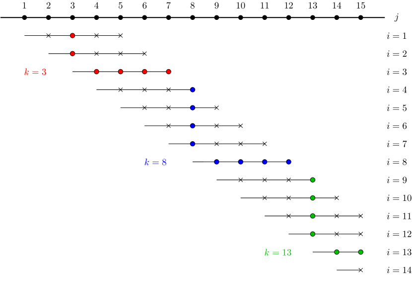
Only the pairs with contribute to . These contributions are called the non-trivial parts for simplicity. The number of these pairs depends on whether belongs to or , as already seen in Remark 2.2. Figure 1 visualizes this case distinction for the exemplary choice of and .
If then the non-trivial parts are
This means is constant due to cancellation, and vanishes when computing the variance. So, in the short case, originates only from and . If then . If , then . So, the overall representation of in the short case is
Therefore,
So, the leading term is always . In light of Theorem 2.3, according to which contains the monomials and it must be ensured that is dominant over . This means . ∎
Now, we consider the long case. Due to we now have , and the regions are redefined according to Remark 2.2. For the non-trivial parts, we note that:
-
•
If or then the non-trivial parts are the same as in the short case.
-
•
If then the non-trivial parts yield .
So, we again obtain a representation in the way of
| (6) |
The proof of the following lemma shows that if then the leading terms of and do not match perfectly.
Proof of Lemma 3.4 for symmetric groups.
From (6), we state that
| (6a) | ||||
| (6b) | ||||
| (6c) |
By appropriate index shifting, we calculate
This gives the total result
In contrast, by Theorem 2.3,
Since the long case implies , all monomials of order 3 are leading terms. The monomials appearing in and appearing in do not match in general. Using , we can write
This shows that we need since otherwise, there are two different leading coefficients of . ∎
We now derive the analogous statements for the other classical Weyl groups and . It is sufficient to prove the lemmas 3.3 and 3.4 for the groups since the difference between and is asymptotically negligible (cf. (5a) and (5b)). Recall the asymptotic quantification of given in Lemma 2.6.
To compute we ignore all constant parts appearing in . By (5a), we can split where
The third sum is asymptotically negligible. So, to obtain a representation we write , with stemming from and stemming from respectively.
For we can use the previous counting method. However, we have to take into account that on ,
In conclusion, the coefficients on are half of the coefficients on . Note that for all . Moreover, where
Recall that by Remark 2.5, the short case is now and the long case is . By counting the number of such and , we can determine the asymptotic quantification of .
Proof of Lemma 3.3 for the groups and .
If , then all pairs in are located within , yielding
In conclusion, if then
Due to according to Lemma 2.6, we obtain the same condition as in Lemma 3.3, namely, .
If , then the pairs in also cover . For there cannot be any pairs if while this is possible if . However, the difference between these two subcases is only marginal. If we obtain
If then
In conclusion, if then
Proof of Lemma 3.4 for the groups and .
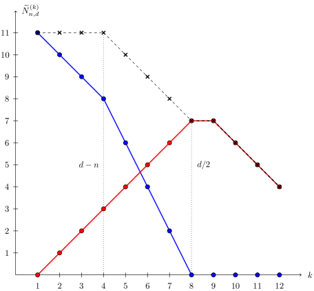
In the long case, the main focus is on counting . Figure 2 illustrates the positions of pairs in the long case for the exemplary choice of .

With help of Figure 2, it is straightforward to count
This result is also illustrated in Figure 3, which displays the number of pairs and the number of pairs .
Therefore, in the long case, we have
We compute
Due to we obtain
On the other hand, by Lemma 2.6,
i.e., the leading terms and need to match. Writing for this gives the condition
which holds precisely for and . ∎
References
- [1] Anders Björner and Francesco Brenti, Combinatorics of Coxeter groups, vol. 231, Springer Science & Business Media, 2006.
- [2] Miklós Bóna, Generalized descents and normality, Electronic Journal of Combinatorics 15 (2008), N21.
- [3] Jinyuan Chang, Xiaohui Chen, and Mingcong Wu, Central limit theorems for high dimensional dependent data, arXiv preprint arXiv:2104.12929 (2021).
- [4] Harold S. M. Coxeter, The complete enumeration of finite groups of the form , Journal of the London Mathematical Society 1 (1935), no. 1, 21–25.
- [5] Filippo de Mari and Mark A. Shayman, Generalized eulerian numbers and the topology of the hessenberg variety of a matrix, Acta Applicandae Mathematica 12 (1988), 213–235.
- [6] Philip Dörr and Johannes Heiny, Extremes of joint inversions and descents on finite coxeter groups, arXiv preprint arXiv:2309.17314 (2023).
- [7] Philip Dörr and Thomas Kahle, Extreme values of permutation statistics, arXiv preprint arXiv:2205.01426 (2022).
- [8] Thomas Kahle and Christian Stump, Counting inversions and descents of random elements in finite Coxeter groups, Mathematics of Computation 89 (2020), no. 321, 437–464.
- [9] Kathrin Meier and Christian Stump, Central limit theorems for generalized descents and generalized inversions in finite root systems, preprint, arXiv:2202.05580 (2022).
- [10] John Pike, Convergence rates for generalized descents, the electronic journal of combinatorics (2011), P236–P236.
- [11] Aad W. van der Vaart, Asymptotic statistics, vol. 3, Cambridge university press, 2000.