Sensing quantum vacuum fluctuations with non-Gaussian electronic noise

Abstract

The statistics of electron transport in a tunnel junction is affected by fluctuations of its voltage bias, which modulates the probability for electrons to cross the junction. We exploit this phenomenon to provide a direct measurement of quantum vacuum fluctuations in the microwave domain of a resistor placed at ultra-low temperature: we show that the amplified vacuum fluctuations are correlated with the noise generated by the junction to contribute to a third moment of detected voltage fluctuations. This experiment constitutes an absolute measurement of noise, not affected by the unavoidable noise added by the detection setup.

I Introduction

Vacuum fluctuations, the fact that the electromagnetic field always fluctuates, even in free space at zero temperature, is a direct consequence of the Heisenberg uncertainty principle, and as such a hallmark of quantum physics. Two consequences are found in most textbooks when calculating the energy levels of the hydrogen atom: the energy levels are shifted, even that of the ground state (Lamb shift), and all excited states acquire a finite lifetime (for a review on the manifestations of vacuum fluctuations, see [1]).

Mesoscopic circuits cooled to ultra-low temperatures and connected to microwave transmission lines bare many similarities with the hydrogen atom in vacuum, to the point that some simple circuits are often nicknamed ”artificial atoms”[2]. Indeed, such circuits with a few degrees of freedom are well described by hamiltonians with a discrete spectrum, and a semi-infinite transmission line (or in practice, terminated by a matched load at low temperature) is nothing but a unidimensional vacuum for electromagnetic waves in the microwave domain[3]. The energy levels of these circuits are shifted and have finite lifetime, a major difficulty for the development of solid state quantum computers[2].

While superconducting circuits such as those used as qubits can be considered similar to atoms, dissipative circuits made of normal conductors, by involving the electronic degrees of freedom, are much more complex, with continuous spectra. Among them the tunnel junction, made of two metallic contacts separated by a thin insulating film through which electrons can tunnel, is among the simplest. Not connected, i.e. purely voltage biased, it has a linear current-voltage characteristic like a simple resistor. Connected to a transmission line, it becomes nonlinear, a phenomenon called Dynamical Coulomb Blockade (DCB)[4], that in some sense is similar to the Lamb shift.

A direct detection of vacuum fluctuations generated by a resistor can be performed with a microwave amplifier. However the noise of the amplifier itself, which usually dominates the total signal, adds to that of the resistor, and there is no way to separate them, i.e. to know how much noise comes from the resistor and how much from the amplifier. By replacing the resistor by a tunnel junction, which noise can be tuned by a dc bias voltage, from vacuum fluctutations at zero bias to pure shot noise at high bias, the spectrum of vacuum fluctuations has been measured up to 10 GHz[5]. At much higher frequencies, a Josephson junction has been used to downconvert the high frequency ($\sim 100$GHz) vacuum fluctuations of its shunt resistor to low frequency noise ($\sim 100$kHz) that has been detected[6].

In this article we explore the effect of vacuum fluctuations on the statistics of the current fluctuations generated by a tunnel junction beyond the average current and variance. The third moment of voltage fluctuations is known to be strongly influenced by the environment of the junction, both through its impedance and noise temperature [7, 8]. We show here that it is directly sensitive to vacuum fluctuations, which modulate the noise of the junction. Correlating vacuum fluctuations and the sample noise, both being first amplified, provides a direct measurement of the variance of the field vacuum fluctuations. In our experiment, the source of vacuum fluctuations is external to the junction, which serves as a voltage-to-noise transducer.

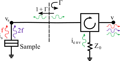
Figure 1: Principle of the detection scheme. Thanks to the circulator, the sample experiences the fluctuations generated by the load $Z_{0}$ (green arrows), which it partially reflects. These induce voltage fluctuations $v_{\text{s}}(t)$ across the sample, which modulate its noise. The detected voltage $v(t)$ contains the noise generated by the sample at frequencies $f$ (red) and $2f$ (blue) as well as the reflected environmental fluctuations at both frequencies (green).

II Theory

How the statistics of current fluctuations in a mesoscopic conductor translates into that of the detected voltage has been shown to be nontrivial beyond the variance [7, 8]. In order to give a clear physical picture of why, we start by omitting frequency dependence in the expressions. We consider the simplified schematics depicted in Fig.1. A fluctuating current $i_{\text{s}}(t)$ generated by the sample leads to a detected voltage $v(t)=\frac{1}{2}Z_{0}(1+\Gamma)i_{\text{s}}(t)$ with $Z_{0}$ the characteristic impedance of the transmission line between the sample and the amplifier matched to it (here $Z_{0}=50\Omega$), and $\Gamma=(R_{\text{s}}-Z_{0})/(R_{\text{s}}+Z_{0})$ the voltage reflection coefficient of a wave impinging onto the sample of resistance $R_{\text{s}}$.

The electromagnetic environment of the sample, modeled by a noise source of impedance $Z_{0}$ generating current fluctuations $i_{\text{env}}(t)$ also contributes to the detected voltage by being partially reflected by the sample, i.e. as $\frac{1}{2}Z_{0}\Gamma i_{\text{env}}$. As a result the third moment of the detected voltage contains, in average over time, two terms:

$$\langle v^{3}\rangle=k[\langle i_{\text{s}}^{3}\rangle+3\frac{\Gamma}{1+\Gamma}\langle i_{\text{s}}^{2}i_{\text{env}}\rangle]$$ (1)

with $k=\frac{Z_{0}^{3}}{8}(1+\Gamma)^{3}$. The first term, $\langle i_{\text{s}}^{3}\rangle$ contains the intrinsic third moment of current fluctuations and the self modulation of the noise, also called feedback term, explained below. The second term corresponds to the modulation of the sample current fluctuations by the time-dependent voltage $v_{\text{s}}(t)$ across the sample coming from the noisy environment. It is given by $\chi\langle v_{\text{s}}i_{\text{env}}\rangle$. Here $\chi\sim d\langle i_{\text{s}}^{2}\rangle/d{V_{\text{s}}}$ is the noise susceptibility which measures how much a small voltage variation modifies the variance of current fluctuations [9, 10], and $\langle v_{\text{s}}i_{\text{env}}\rangle=\frac{1}{2}(1+\Gamma)Z_{0}\langle i_{\text{env}}^{2}\rangle$. The feedback term mentioned above corresponds to the same mechanism, replacing $i_{\text{env}}$ by $i_{\text{s}}$. While $\langle i_{\text{s}}^{3}\rangle$ and $\chi$ may have complex frequency dependence in the quantum regime at low voltage [9, 10, 11, 12, 13, 14, 15], they are simple in the classical limit of pure shot noise, where the bias voltage across the sample $V_{\text{s}}$ is the largest energy scale, $eV_{\text{s}}\gg hf,k_{B}T$ with $T$ the sample temperature. In this limit the electrons follow a Poisson statistics with current fluctuations having spectral densities given by $e\absolutevalue{I_{\text{s}}}$ for the variance and $e^{2}I_{\text{s}}$ for the third moment, both frequency independent. $I_{\text{s}}=V_{\text{s}}/R_{\text{s}}$ is the average, dc bias current in the junction. The noise susceptibility is simply $\chi=d(e\absolutevalue{I_{\text{s}}})/dV_{s}=\text{sign}(I_{\text{s}})e/R_{\text{s}}$. Our experiment corresponds to the situation where the sample is classical but the electromagnetic environment is quantum, i.e. can be in the vacuum state. In this limit the sample acts as a transducer of vacuum fluctuations into a modulation of the classical noise it generates.

We now introduce the frequency dependence. The spectral density of the third moment of the detected voltage fluctuations involves three frequencies, $\langle v(f_{1})v(f_{2})v(f_{3})\rangle$. Time-averaging in the absence of an ac excitation imposes $f_{1}+f_{2}+f_{3}=0$. In the following we will consider the special case where only two frequencies are involved in the detection, $f_{1}=f_{2}=f$, $f_{3}=-2f$, which simplifies the detection. Restoring the frequency dependence of the quantities, we find in the limit $\absolutevalue{eV_{\text{s}}}\gg hf,k_{B}T$:

$$\langle v(f)^{2}v(-2f)\rangle=k\quantity[(3x-1)e^{2}I_{\text{s}}+\text{sign}(I_{\text{s}})\frac{\Gamma}{2}\frac{Z_{0}}{R_{\text{s}}}e\tilde{S}_{\text{env}}(f)]$$ (2)

with $x=\frac{1}{2}(Z_{0}/R_{\text{s}})(1+\Gamma)=Z_{0}/(R_{\text{s}}+Z_{0})$ and

$$\tilde{S}_{\text{env}}(f)=2S_{\text{eq}}(f)+S_{\text{eq}}(2f)$$ (3)

with $S_{\text{eq}}(f)=(hf/Z_{0})\coth{(hf/2k_{B}T_{\text{env}})}$ the current spectral density of equilibrium noise, thermal and quantum, of a resistor $Z_{0}$ at temperature $T_{\textrm{env}}$[3]. $\tilde{S}_{\text{env}}$ is $6k_{B}T_{\text{env}}/Z_{0}$ at high temperature ($k_{B}T_{\text{env}}\gg hf$) and corresponds to vacuum fluctuations, $\tilde{S}_{\text{env}}=4hf/Z_{0}$ at low temperature ($k_{B}T_{\text{env}}\ll hf$). As obvious in Eq. (2), the third moment of the detected voltage at frequencies $(f,-2f)$ is a linear function of the bias current with an offset proportional to $\tilde{S}_{\text{env}}$, i.e. $\expectationvalue{v(f)^{2}v(-2f)}\propto Z_{0}^{3}e^{2}(I_{\text{s}}+I_{0})$ with:

$$eI_{0}=\frac{\Gamma Z_{0}}{2R_{\text{s}}(1-3x)}\tilde{S}_{\text{env}}.$$ (4)

The offset $I_{0}$ is the quantity we have measured, it is a direct measurement of the variance of vacuum fluctuations.

III Experimental setup

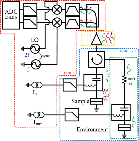
Figure 2: Experimental setup for experiment I. The dashed blue box indicates the low temperature stage of the dilution refrigerator, which temperature can be controlled from 10mK to 1K. The dashed green box is the electromagnetic environment, which noise influences the sample. In experiment II, it is replaced by a 50$\Omega$ resistor with no connection to room temperature.

It is usually best for microwave measurements to have the sample matched to the transmission lines, i.e. $\Gamma=0$. Unfortunately, this washes out the effect we seek to measure, see Eq.(2): it is essential for the vacuum fluctuations generated by the environment to be reflected by the sample in order to be amplified and detected. We chose to work in the limit $R_{\text{s}}\gg Z_{0}$, i.e. the amplifier is almost an ammeter for the sample. The sample used for this experiment is a 4 µm² Al-Al₂O₃ tunnel junction with a dc resistance of $R_{\text{s}}=505\Omega$. The junction is fabricated on a high resistivity, oxidized Si substrate in a single photo-lithography step by doing shadow evaporation of Al through a Dolan bridge [16] using e-beam deposition. The sample is exposed to oxygen to oxidize the Al and create the Al₂O₃ barrier. The junction is placed between the center conductor and ground plane of a 50$\Omega$ CPW transmission line made of 300nm thick Al, wire bonded to a microwave sample holder. The substrate is glued on the sample holder with silver paste. A strong permanent magnet placed under the sample holder keeps the Al into its normal, non-superconducting state.

The setup is shown in Fig. 2. The sample holder is anchored on the 10mK stage of a dilution refrigerator. A bias-tee separates the dc current used to bias the junction from the high frequency noise generated by the junction. A two-stage 4-12 GHz circulator provides a 36dB isolation between the 4K plate of the refrigerator and the junction. It insures that, at the detection frequencies, the sample experiences only vacuum fluctuations at the lowest temperatures, and not thermal noise of an uncontrolled temperature, such as the one coming from the amplifier. The noise generated by the sample together with the environmental noise reflected by the sample are amplified through a 1-12 GHz low-noise HEMT amplifier placed at 4K. At room temperature, this signal is separated into two bands around $f=5.05$GHz and $2f=10.1$GHz using a combination of diplexer and filters. These two signals are downconverted using two mixers with phase-locked microwaves sources as local oscillators at $f$ and $2f$, low-pass filtered below 117MHz and digitized using synchronized 14 bits, 400 MSample/s analog-to-digital converters. In the following we will note $X_{f}(t)$ and $X_{2f}(t)$ the signals digitized after demodulation at frequencies $f$ and $2f$, i.e. the in-phase quadratures.

After a 256 MSample acquisition on both channels, the 2D histogram of $(X_{f},X_{2f})$ is computed, from which the relevant moments of the distribution of $X_{f}$ and $X_{2f}$ are deduced: the variances at frequencies $f$, $\expectationvalue{X_{f}^{2}}$, and $2f$, $\expectationvalue{X_{2f}^{2}}$ and the correlator $\expectationvalue{X_{f}^{2}X_{2f}}$ which we will denote $\expectationvalue{X^{3}}$ for the sake of brevity. The absolute phase of the measurements has no influence since the sample does not experience any ac excitation, so $\expectationvalue{X_{f}^{2}}=\expectationvalue{Y_{f}^{2}}\propto S_{2}(f)$ with $Y$ the other quadrature of the signal at frequency $f$, and $S_{2}$ the noise spectral density. Similarly, $\expectationvalue{X_{2f}^{2}}=\expectationvalue{Y_{2f}^{2}}\propto S_{2}(2f)$. In contrast, the relative phase between the local oscillators at $f$ and $2f$ matters. We chose it so that $\expectationvalue{X_{f}^{2}Y_{2f}}=0$, i.e. $\expectationvalue{X^{3}}$ is proportional to the real part of $\expectationvalue{v(f)^{2}v(-2f)}$ (for more details, see appendix B). While non-linearities in the setup have negligible effects on the measurement of $\expectationvalue{X_{f}^{2}}$ and $\expectationvalue{X_{2f}^{2}}$, they add extra contributions to $\expectationvalue{X^{3}}$ which can be polluted by a term of order 4, in particular $\expectationvalue{X_{f}^{2}X_{2f}^{2}}$. These terms are even functions of the bias current $I_{s}$. To remove them from $\expectationvalue{X^{3}}$, which is an odd function of the bias current, we simply anti-symmetrize it with respect to $I_{\text{s}}$ [7, 11]. For example for the low temperature curve of Fig. 3, the even part is only a constant, -1mV³.

We have performed two experiments corresponding to different environments. In experiment I, the environment consists of a 10dB attenuator followed by another tunnel junction, the environmental junction (of resistance $45\Omega)$, see Fig.2. In the absence of bias, this environment is equivalent to a pure resistor as in Eq.(3). A dc current $I_{\text{env}}$ applied to the environmental junction allows to tune its noise while keeping the fridge at 10mK. The 10dB attenuator inserted between the junction and the circulator insures a good impedance match of the junction and attenuates the noise sent by the environmental junction towards the sample. As a result, the total noise $\tilde{S}_{\text{env}}$ experienced by the sample consists of the equilibrium noise of the attenuator plus the attenuated shot noise of the environmental junction. In the limit $eV_{\text{env}}>hf$, this reads:

$$\tilde{S}_{\text{env}}(f)=\alpha eI_{\text{env}}+(1-\alpha)[2S_{\text{eq}}(f)+S_{\text{eq}}(2f)]$$ (5)

with $\alpha$ the attenuation factor between the two junctions. In experiment II, the environment simply consists of a cryogenic, macroscopic $50\Omega$ resistor thermalized on the base plate of the refrigerator. Its temperature is close to that of the fridge, which is controlled from 10mK to 0.6K. In this experiment, the noise experienced by the sample is modified by changing the temperature of the refrigerator, i.e. also that of the sample.

IV Results

Measurements of $\expectationvalue{X_{f}^{2}}$ and $\expectationvalue{X_{2f}^{2}}$ as a function of the sample bias current $I_{s}$ allow to determine the electron temperature $T$ of the sample [17]. We find that $T$ is identical to the fridge temperature except at the lowest temperatures (we obtain $T=20$mK at the base temperature), see appendix C. The temperature of the sample is however irrelevant for us since we operate it at high bias, where it is generating purely shot noise, i.e. $S_{2}(f)=S_{2}(2f)=e\absolutevalue{I_{\text{s}}}$. Measurements of the third order correlator $\expectationvalue{X^{3}}$ as a function of $I_{\text{s}}$ in experiment I are reported in Fig. 3, for various biases of the environmental junction, i.e. various environmental noises. For $I_{\mathrm{env}}=0$, we show the measurement of the full bias dependence (symbols), in very good agreement with theory (red dashed line, see appendix A). To our knowledge, this represents the first measurement of a third order correlator of noise in a mesoscopic device in a fully quantum regime, in which every frequency involved is greater than both $k_{B}T/h$ and $eV/h$. Here the only unknown parameter is the overall gain of the setup. In the following we consider only the classical, high bias limit of this curve, which corresponds to Eq.(2). As discussed above, we indeed observe that the high bias behaviour of $\expectationvalue{X^{3}}$ is linear with an offset, i.e. $\expectationvalue{X^{3}}\propto(I_{\text{s}}+I_{0})$.

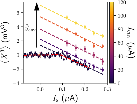
Figure 3: Examples of $\expectationvalue{X^{3}}$ vs. bias current $I_{s}$ in the sample for different environmental conditions in experiment I. Different colors correspond to different current bias in the environmental junction, see the color scale on the right. The dashed lines are linear fits from which we extract $\tilde{S}_{\text{env}}$. The red dashed line is the theoretical prediction for $\expectationvalue{X^{3}}$ when the junction is exposed to vacuum fluctuations, see appendix A.

Acquiring the data shown in Fig.3 for $I_{\text{env}}=0$, i.e. with the full dependence on $I_{\text{s}}$ takes about 2 weeks. While we considered important to do this measurement at the lowest temperature to make sure that the experiment is well controlled, it is irrelevant to the final goal of the experiment, i.e. determining $I_{0}$ as a function of the environmental noise. For this all is needed are a few points in the high $I_{\text{s}}$ regime to determine how the offset is affected. We show in Fig.3 a few examples of such a determination for various environmental bias currents (experiment I). As expected, changing $I_{\text{env}}$ only shifts the curves without changing their slope. We have repeated this procedure to determine $I_{0}$ as a function of $I_{\text{env}}$ (experiment I) or $T$ (experiments I and II).

From the measurement of $I_{0}$ we deduce the environmental noise spectral density $\tilde{S}_{\text{env}}$ using Eq.(4). Fig. 4 shows the measured dependence of $\tilde{S}_{\text{env}}$ with $I_{\text{env}}$ (between 0 and $120\mu$A, experiment I) and the electron temperature $T$ (between 20mK and 600mK, experiments I and II).

We first discuss the dependence on $I_{\textrm{env}}$, i.e. the green symbols (data) and green dashed line (theory) vs. upper scale in Fig. 4. The environmental junction is always biased in its classical limit so the noise it generates is pure shot noise $e\absolutevalue{I_{\textrm{env}}}$ both at frequencies $f$ and $2f$ ($eV_{\textrm{env}}=hf$ corresponds to $I_{\textrm{env}}\simeq 0.5\mu$A). This noise is partially coupled to the microwave circuitry, attenuated by the 10dB attenuator and further attenuated by the circuitry between the two junctions. As already discussed, $\tilde{S}_{\text{env}}$ grows linearly with $I_{\text{env}}$, according to Eq. (5), in good agreement with our observations. The observed slope $\alpha=0.0536$ corresponds to an effective attenuation of 17.5dB. An independent estimation of $\alpha$ from $\expectationvalue{X_{f}^{2}}$ and $\expectationvalue{X_{2f}^{2}}$ measurements vs. $I_{\text{env}}$ at $I_{\text{s}}=0$ gives an attenuation of 17.2dB, see appendix C.

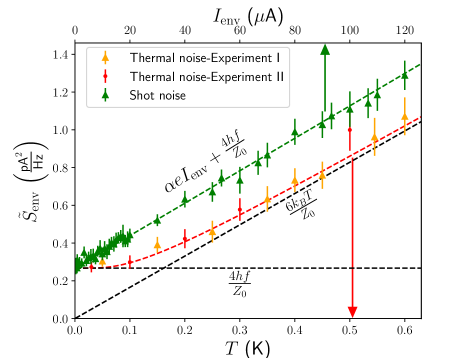
Figure 4: Environmental noise $\tilde{S}_{\text{env}}$ vs. environmental bias current (experiment I, upper x scale) or environmental temperature (experiments I and II, lower x scale). Green triangles are the data corresponding to varying $I_{\text{env}}$ in experiment I. Orange triangles are the data corresponding to varying the temperature while keeping $I_{\text{env}}=0$ in experiment I. Red dots are the data corresponding to varying the temperature in experiment II, where the environment is a 50$\Omega$ resistor. The black horizontal (resp. oblique) dashed line corresponds to the theoretical limit of zero temperature quantum noise (resp. high temperature thermal noise). The red dotted line is the theoretical prediction for $\tilde{S}_{\text{env}}$ according to Eq.(3).

We now consider the same setup in which we do not bias the environmental junction but vary the temperature of the refrigerator. The corresponding data are shown as orange triangles in Fig.4. As clearly seen in the data, the behaviour goes from a linear temperature dependence with no offset at high T (black dotted line labelled ”$6k_{B}T/Z_{0}$”) to a saturation at low T (black dotted line labelled ”$4hf/Z_{0}$”). This corresponds to the environmental noise going from thermal at high T to quantum, reduced to vacuum fluctuations, at low T. The theoretical prediction of Eq.(3), shown with no fitting parameter as a red dashed line in Fig.4, is in very good agreement with the measurement.

As discussed before, the bias-dependence of the noise generated by tunnel junctions is an excellent electron thermometer. This allows us to confirm we are not simply measuring the lack of thermalization of electrons at very low temperature. We find for the sample $T=20$mK at base temperature. We have also measured the noise of the environmental junction vs. $I_{\textrm{env}}$ reflected by the sample while keeping $I_{\text{s}}$ constant. We find an electron temperature for the environmental junction of 23mK. In experiment II, the environmental noise source is simply a macroscopic $50\Omega$ load well thermalized to the base plate of the refrigerator. Corresponding data are shown in Fig.4 as red circles. These data corroborate what has been measured in experiment I, thus confirming that our experiment constitutes an absolute meter of electromagnetic fluctuations.

V Conclusion

We have measured the impact of a controlled electromagnetic noise on the current statistics of a tunnel junction by studying its effect on the measured third moment. We have observed that even the unavoidable quantum vacuum fluctuations have a strong influence on of electron transport beyond the usual dc current and variance. This demonstrates that our setup constitutes an in-situ absolute noise detector at cryogenic temperature that could be used for many other studies. In our experiment the sample was biased in its classical regime, yet sensitive to quantum fluctuations. What happens to higher order statistics of electron quantum transport in the presence of a quantum electromagnetic field (vacuum, squeezed state, etc.) is a fully open problem [18]. Our experiment paves the way to its exploration.

Appendix A Noise susceptibility and the full current dependence of $\expectationvalue{X^{3}}$

The main tool we have used to detect vacuum fluctuations is the noise susceptibility $\chi$, the response of noise to an excitation. For this, we only considered the high voltage regime ($eV_{\text{s}}\gg k_{B}T,hf$), in which case $\chi$ is simply given by $\derivative{S_{2}}{V_{\text{s}}}$. However, in the quantum regime ($eV_{\text{s}}<hf$ and $hf\gg k_{B}T$) the noise susceptibility is more complex, and particular it acquires a dependence on the excitation frequency $f_{0}$ and detection frequency $f$. It is defined by [9]:

$$\chi_{f_{0}}(f)=\lim_{v_{\text{s}}\to 0}\frac{\expectationvalue{i_{\text{s}}(f)i_{\text{s}}(f_{0}-f)}}{v_{\text{s}}}$$

and gives [9, 10]:

$$\chi_{f_{0}}(f)=\frac{e}{2hf_{0}}\big{(} S_{2}^{0}(f_{+})-S_{2}^{0}(f_{-})$$

$$+S_{2}^{0}(f_{-}-f_{0})-S_{2}^{0}(f_{+}-f_{0})\big{)}$$

with $f_{\pm}=f\pm\frac{eV_{\text{s}}}{h}$. Here we use $S_{2}^{0}(f)=\frac{hf}{R_{\text{s}}}\coth(\frac{hf}{2k_{B}T})$ the equilibrium noise given by the fluctuation-dissipation theorem. This result has been confirmed experimentally for $f\sim f_{0}$ [9] and very recently for $f\sim-f_{0}$ and $f\sim 2f_{0}$ [12], which are the relevant conditions for our experiment.

Since the final model describes very well our data, we will work with the assumption that the sample’s impedance is purely resistive and ignore any reactive component, $Z_{\text{s}}(f)=R_{\text{s}}$. In order to describe the measured third moment, we first consider the input voltage $v$ into the amplifier as well as the fluctuating voltage across the sample $v_{\text{s}}$. They are given by:

$$v(f) =\frac{1}{2}Z_{0}\left[-(1+\Gamma)i_{\text{s}}(f)+\Gamma i_{\text{env}}(f)\right]$$

$$v_{\text{s}}(f) =\frac{1}{2}Z_{0}(1+\Gamma)\left[-i_{\text{s}}(f)+i_{\text{env}}(f)\right]$$

Here $Z_{0}=50\Omega$ is the characteristic impedance of the transmission lines in the circuit, matched to the resistance of the environment. The third moment of the detected voltage fluctuations, obtained by correlating the square of the voltage at frequency $f$ with the voltage at frequency $f$, i.e. $S_{3,V}=\expectationvalue{v^{2}(f)v(-2f)}$, is given by:

$$S_{3,V}= -Z_{/\!/}^{3}\expectationvalue{i_{\text{s}}^{2}(f)i_{s}(-2f)}_{V_{\text{s}}+v_{\text{s}}}$$

$$+\frac{1}{2}Z_{/\!/}^{2}\Gamma Z_{0}\bigg{(}\expectationvalue{i_{\text{s}}^{2}(f)i_{\text{env}}(-2f)}_{V_{\text{s}}+v_{\text{s}}}$$

$$\qquad+2\expectationvalue{i_{\text{s}}(f)i_{\text{s}}(-2f)i_{\text{env}}(f)}_{V_{\text{s}}+v_{\text{s}}}\bigg{)}$$

with $Z_{/\!/}=\frac{1}{2}Z_{0}(1+\Gamma)=\frac{R_{\text{s}}Z_{0}}{R_{\text{s}}+Z_{0}}$. We added the subscript $V_{\text{s}}+v_{\text{s}}$ to indicate that the sample experienced a time-dependent voltage being the sum of the applied dc one $V_{\text{s}}$ plus the fluctuating $v_{\text{s}}(t)$. Following [8, 11], one has:

$$\expectationvalue{i_{\text{s}}^{2}(f)i_{\text{s}}(-2f)}_{V_{\text{s}}+v_{\text{s}}}= \expectationvalue{i_{\text{s}}^{2}(f)i_{\text{s}}(-2f)}_{V_{\text{s}}}$$

$$+\expectationvalue{\expectationvalue{i_{\text{s}}^{2}(f)}i_{\text{s}}(-2f)}$$

$$+2\expectationvalue{\expectationvalue{i_{\text{s}}(f)i_{\text{s}}(-2f)}i_{\text{s}}(f)}$$

$$= S_{3,I}+\chi_{2f}(f)\expectationvalue{v_{\text{s}}(2f)i_{\text{s}}(2f)}$$

$$+2\chi_{-f}(f)\expectationvalue{v_{\text{s}}(-f)i_{\text{s}}(f)}$$

$$= S_{3,I}-Z_{/\!/}\chi_{2f}(f)S_{2}(2f)$$

$$-2Z_{/\!/}\chi_{-f}(f)S_{2}(f).$$

$S_{3,I}$ is the intrinsic third moment of current fluctuations, corresponding to the Poissonian statics of the tunneling electrons. A complete quantum treatment gives $S_{3,I}=e^{2}I$ [13, 14, 15], independent of frequency. $S_{2}(f)$ is the usual current noise spectral density of shot noise for a tunnel junction[19]:

$$S_{2}(f)=\frac{1}{2}\quantity[S_{2}^{0}\quantity(f+\frac{eV_{\text{s}}}{h})+S_{2}^{0}\quantity(f-\frac{eV_{\text{s}}}{h})].$$ (6)

Repeating the same steps with the other two terms gives us:

$$\expectationvalue{i_{\text{s}}^{2}(f)i_{\text{env}}(-2f)} =Z_{/\!/}\chi_{2f}(f)S_{2}^{\text{env}}(2f)$$

$$\expectationvalue{i_{s}(f)i_{\text{s}}(-2f)i_{\text{env}}(f)} =Z_{/\!/}\chi_{-f}(f)S_{2}^{\text{env}}(f).$$

As explained in the main article, the environmental noise source $S_{2}^{\text{env}}$ is either equilibrium noise, as given by $S_{2}^{0}$ for a resistance $Z_{0}$ , or the shot noise coming from a second tunnel junction. In the end, $S_{3,V}=S_{3}^{\text{int}}+S_{3}^{\text{fb}}+S_{3}^{\text{env}}$ with:

$$S_{3}^{\text{int}} =-Z_{/\!/}^{3}S_{3,I}$$

$$S_{3}^{\text{fb}} =Z_{/\!/}^{4}\quantity[\chi_{2f}(f)S_{2}(2f)+2\chi_{-f}(f)S_{2}(f)]$$

$$S_{3}^{\text{env}} =\frac{1}{2}Z_{/\!/}^{3}\Gamma Z_{0}\quantity[\chi_{2f}(f)S_{2}^{\text{env}}(2f)+2\chi_{-f}(f)S_{2}^{\text{env}}(f)].$$

As will be shown in the next section, the measured signal $\expectationvalue{X^{3}}$ is proportional to $S_{3,V}$. Since the electron temperature is known from the measurement of $S_{2}$, we can predict the full current dependence of $S_{3,V}$ up to an overall gain factor. Our data are in very good agreement with the theoretical prediction, see Fig. 5.

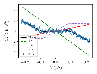
Figure 5: Third moment of voltage fluctuations. Blue symbols are data (the one already presented in the main article) and the black solid line is the theoretical prediction. The theory is the sum of three terms, the intrinsic (dashed green), environmental (dashed violet) and feedback (dashed red).

Appendix B Downconversion and integration over the bandwidth

We now want to illustrate how the measured voltages, $X_{f}(t)$ and $X_{2f}(t)$, allow us to find $S_{3,V}$. Before the downconversion, the signals in both channels, $s_{f}$ and $s_{2f}$, can be written as an integral over a bandwidth $\Delta$, the same for both signals. The overall transfer function $G(f)$ is a function of frequency and is complex.

$$s_{f}(t) =\int_{-\Delta}^{+\Delta}d\epsilon\quantity(G(f+\epsilon)v(f+\epsilon)e^{i2\pi(f+\epsilon)t}+\text{c.c.})$$

$$s_{2f}(t) =\int_{-\Delta}^{+\Delta}d\epsilon\quantity(G(2f+\epsilon)v(2f+\epsilon)e^{i2\pi(2f+\epsilon)t}+\text{c.c.})$$

The mixers multiply these 2 signals with in-phase local oscillators. The low pass filters remove the high frequency components, so we will simply ignore components at frequencies close to $2f$ for $X_{f}$ and $4f$ for $X_{2f}$.

$$X_{f}(t) =s_{f}(t)\cdot\cos(2\pi ft)$$

$$=\frac{1}{2}\int_{-\Delta}^{+\Delta}d\epsilon\quantity(G(f+\epsilon)v(f+\epsilon)e^{i2\pi\epsilon t}+\text{c.c.})$$

$$X_{2f}(t) =\frac{1}{2}\int_{-\Delta}^{+\Delta}d\epsilon\quantity(G(2f+\epsilon)v(2f+\epsilon)e^{i2\pi\epsilon t}+\text{c.c.})$$

$$\expectationvalue{X^{3}} =\expectationvalue{X_{f}^{2}X_{2f}}$$

$$=\frac{1}{8}\int d\epsilon d\epsilon^{\prime}d\epsilon^{\prime\prime}\bigg{(}G(f+\epsilon)G(f+\epsilon^{\prime})G(-2f-\epsilon^{\prime\prime})$$

$$\cdot \expectationvalue{v(f+\epsilon)v(f+\epsilon^{\prime})v(-2f-\epsilon^{\prime\prime})}e^{i2\pi(\epsilon+\epsilon^{\prime}-\epsilon^{\prime\prime})t}+\text{c.c.}\bigg{)}$$

$$=\frac{1}{8}\int d\epsilon d\epsilon^{\prime}d\epsilon^{\prime\prime}\bigg{(}G(f+\epsilon)G(f+\epsilon^{\prime})G(-2f-\epsilon^{\prime\prime})$$

$$\cdot S_{3,V}(f+\epsilon,f+\epsilon^{\prime})\delta(\epsilon+\epsilon^{\prime}-\epsilon^{\prime\prime})e^{i2\pi(\epsilon+\epsilon^{\prime}-\epsilon^{\prime\prime})t}+\text{c.c.}\bigg{)}$$

$$=\frac{1}{4} \int d\epsilon d\epsilon^{\prime}\text{Re}\quantity(G(f+\epsilon)G(f+\epsilon^{\prime})G(-2f-\epsilon-\epsilon^{\prime})S_{3,V}(f+\epsilon,f+\epsilon^{\prime}))$$

The last line corresponds to a time average and reflects the fact that the third order correlator has to respect the frequency summation rule. To measure its imaginary part, we can instead turn to $\expectationvalue{X_{f}^{2}Y_{2f}}$, with $Y_{2f}(t)=s(t)\cdot\sin(2\pi 2ft)$. While not measured for this sample, we measured the imaginary part of $S_{3,V}$ to be indeed zero, as predicted by the theory (data not shown). The bandwidth $\Delta\sim 100$MHz is narrow enough so that $S_{3,V}(f,f)$ does not vary significantly within it. Thus, $\expectationvalue{X^{3}}=AS_{3,V}(f,f)$ with:

$$A=\frac{1}{4}\int d\epsilon d\epsilon^{\prime}\text{Re}[G(f+\epsilon)G(f+\epsilon^{\prime})G(-2f-\epsilon-\epsilon^{\prime})]$$

A severe difficulty in the measurement of $S_{3,V}(f,f)$ is to make sure that the phases of $G(f)$ and $G(2f)$ do not vary much within the detection bandwidth, up to an overal delay. Indeed, not only the power gain matters, and a quickly rotating phase makes the parameter $A$ vanish. A pump tone sent onto the sample, as in [12], allows us to characterize $G$ and helps testing the detection scheme.

Appendix C Electron temperature

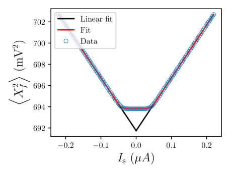
Figure 6: Variance $\expectationvalue{X_{f}^{2}}$ as a function of the bias current in the sample. The fit allows to determine the electron temperature of the sample.

We deduce the electron temperature in the sample from the measurements of its noise spectral density $S_{2}$, extracted from the variances $\expectationvalue{X_{f}^{2}}$ and $\expectationvalue{X_{2f}^{2}}$. Fig. 6 presents the data for $\expectationvalue{X_{f}^{2}}$ for the same acquisition as for the data presented in Fig.5. A linear fit when $eV_{s}\gg hf,k_{B}T$ allows us to find the power gain and the amplifier noise. Fitting the rescaled data with Eq.(6) provides the electron temperature. Qualitatively, the temperature is given by the rounding of the curve near the edges of the plateau, at $eV\sim hf$ or $eV\sim 2hf$. The data of Fig. 6, correspond to $T=19$mK (measured at frequency $f$). From the measurement of $\expectationvalue{X_{2f}^{2}}$ we obtain $T=21$mK measured at frequency $2f$. We find that the electron temperature is always very close to that of the fridge except at the lowest temperature, where we obtain $T\simeq 20$mK whereas the thermometer of the low temperature stage of the refrigerator indicates 10mK.

We can similarly determine the electron temperature of the environmental junction (experiment I), which noise is reflected on the sample and is detected together with that of the sample. Fig. 7 shows $\expectationvalue{X_{f}^{2}}$ as a function of the current bias in the environmental junction for a fixed current $I_{\text{s}}=0$ in the sample. These data correspond to T=23mK. The environmental junction is well thermalized to the fridge except at the lowest temperature.

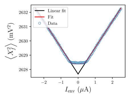
Figure 7: Variance $\expectationvalue{X_{f}^{2}}$ as a function of the bias current in the environmental junction. The fit allows to determine the electron temperature of the environmental junction.

The slope in Fig. 6 corresponds to $G(f)(1-\Gamma^{2})R_{\text{s}}eI_{\text{s}}$. That in Fig. 7 to $G(f)\alpha(f)\Gamma^{2}Z_{0}eI_{\text{env}}$ (however the data in the two figures correspond to setups with different gains). The ratio of the two gives $\alpha(f)$, the attenuation between the environmental junction and the sample at frequency $f$. $\alpha(2f)$ is determined similarly. We then deduce $\alpha=2\alpha(f)+\alpha(2f)$, since $\tilde{S}_{\text{env}}=2S_{2}^{\text{env}}(f)+S_{2}^{\text{env}}(2f)$. With this we find an overall attenuation of $\alpha$=17.2dB. If we take into account the attenuator and the 4mm long wirebond on the environmental junction, this leads to an expected attenuation of 15.5dB, i.e. the circuitry adds another $\sim$2dB of attenuation, a very reasonable number.

References

- Milonni [1993] P. Milonni, The Quantum Vacuum (Academic Press, 1993).
- Blais et al. [2021] A. Blais, A. L. Grimsmo, S. M. Girvin, and A. Wallraff, Circuit quantum electrodynamics, Rev. Mod. Phys. 93, 025005 (2021).
- Callen and Welton [1951] H. B. Callen and T. A. Welton, Irreversibility and generalized noise, Phys. Rev. 83, 34 (1951).
- Ingold and Nazarov [1992] G.-L. Ingold and Y. V. Nazarov, Charge tunneling rates in ultrasmall junctions, in Single Charge Tunneling: Coulomb Blockade Phenomena In Nanostructures, edited by H. Grabert and M. H. Devoret (Springer US, Boston, MA, 1992) pp. 21–107.
- Thibault et al. [2015] K. Thibault, J. Gabelli, C. Lupien, and B. Reulet, Pauli-heisenberg oscillations in electron quantum transport, Phys. Rev. Lett. 114, 236604 (2015).
- Koch et al. [1981] R. H. Koch, D. J. Van Harlingen, and J. Clarke, Observation of zero-point fluctuations in a resistively shunted josephson tunnel junction, Phys. Rev. Lett. 47, 1216 (1981).
- Reulet et al. [2003] B. Reulet, J. Senzier, and D. E. Prober, Environmental effects in the third moment of voltage fluctuations in a tunnel junction, Phys. Rev. Lett. 91, 196601 (2003).
- Beenakker et al. [2003] C. W. J. Beenakker, M. Kindermann, and Y. V. Nazarov, Temperature-dependent third cumulant of tunneling noise, Phys. Rev. Lett. 90, 176802 (2003).
- Gabelli and Reulet [2008] J. Gabelli and B. Reulet, Dynamics of quantum noise in a tunnel junction under ac excitation, Phys. Rev. Lett. 100, 026601 (2008).
- Gabelli and Reulet [2007] J. Gabelli and B. Reulet, The noise susceptibility of a coherent conductor, in Noise and Fluctuations in Circuits, Devices, and Materials, Vol. 6600, International Society for Optics and Photonics (SPIE, 2007) p. 66000T.
- Gabelli et al. [2013] J. Gabelli, L. Spietz, J. Aumentado, and B. Reulet, Electron–photon correlations and the third moment of quantum noise, New Journal of Physics 15, 113045 (2013).
- Farley et al. [2023] C. Farley, E. Pinsolle, and B. Reulet, Noise dynamics in the quantum regime, in 2023 International Conference on Noise and Fluctuations (ICNF) (2023) pp. 1–4.
- Galaktionov et al. [2003] A. V. Galaktionov, D. S. Golubev, and A. D. Zaikin, Statistics of current fluctuations in mesoscopic coherent conductors at nonzero frequencies, Phys. Rev. B 68, 235333 (2003).
- Salo et al. [2006] J. Salo, F. W. J. Hekking, and J. P. Pekola, Frequency-dependent current correlation functions from scattering theory, Phys. Rev. B 74, 125427 (2006).
- Bednorz and Belzig [2010] A. Bednorz and W. Belzig, Models of mesoscopic time-resolved current detection, Phys. Rev. B 81, 125112 (2010).
- Dolan [1977] G. J. Dolan, Offset masks for lift‐off photoprocessing, Applied Physics Letters 31, 337 (1977), https://doi.org/10.1063/1.89690 .
- Spietz et al. [2003] L. Spietz, K. W. Lehnert, I. Siddiqi, and R. J. Schoelkopf, Primary electronic thermometry using the shot noise of a tunnel junction, Science 300, 1929 (2003), https://www.science.org/doi/pdf/10.1126/science.1084647 .
- Souquet et al. [2014] J.-R. Souquet, M. J. Woolley, J. Gabelli, P. Simon, and A. A. Clerk, Photon-assisted tunnelling with nonclassical light, Nature Communications 5, 5562 (2014).
- Blanter and Büttiker [2000] Y. Blanter and M. Büttiker, Shot noise in mesoscopic conductors, Physics Reports 336, 1 (2000).