Large Language Models to the Rescue: Deadlock Resolution in Multi-Robot Systems

Abstract

Multi-agent robotic systems are prone to deadlocks in an obstacle environment where the system can get stuck away from its desired location under a smooth low-level control policy. Without an external intervention, often in terms of a high-level command, it is not possible to guarantee that just a low-level control policy can resolve such deadlocks. Utilizing the generalizability and low data requirements of large language models (LLMs), this paper explores the possibility of using LLMs for deadlock resolution. We propose a hierarchical control framework where an LLM resolves deadlocks by assigning a leader and direction for the leader to move along. A graph neural network (GNN) based low-level distributed control policy executes the assigned plan. We systematically study various prompting techniques to improve LLM’s performance in resolving deadlocks. In particular, as part of prompt engineering, we provide in-context examples for LLMs. We conducted extensive experiments on various multi-robot environments with up to 15 agents and 40 obstacles. Our results demonstrate that LLM-based high-level planners are effective in resolving deadlocks in MRS.

I Introduction

Multi-agent robotic systems (MRS) are widely used in various applications today such as warehouse operations [1, 2], self-driving cars [3], and coordinated navigation of drones in a dense forest for search-and-rescue missions [4], among others. Ensuring safety in terms of collision and obstacle avoidance and scalability to large-scale multi-agent problems are crucial requirements of the control design of MRS. Furthermore, in certain applications of MRS for navigating in unknown environments such as coverage [5] and formation control [6], it is also required that the robot agents remain connected for sharing information and building team knowledge. Existing methods for multi-agent coordination and motion planning are incapable of solving such problems that consider all these aspects, i.e., safety, connectivity, and performance, in terms of reaching a goal destination or following a given trajectory, in a scalable manner.

Figure 1: Overview of the hierarchical control framework. LLM-based high-level planner assigns a leader for the MRS, resulting in a leader-follower formation. A GNN-based low-level controller provides a distributed control policy for safety and connectivity while the leader helps evade the deadlock.

For robotic systems, control barrier functions (CBFs) have become a popular tool to encode safety requirements [7]. The resulting CBF-based quadratic programs (QPs) have gained popularity for control synthesis as QPs can be solved efficiently for real-time control synthesis [8]. While such hand-crafted CBF-QPs have shown promising results when it comes to the safety of single-agent systems [8] and small-scale multi-agent systems [9], it is difficult, if not impossible, to synthesize a CBF when it comes to large-scale MRS under multi-objective problems in environments consisting of numerous obstacles.

In recent years, learning-based methods have shown promising results in computing a CBF for complex nonlinear dynamical systems [10, 11]. Interested readers are referred to the recent survey [12] on learning-based methods for safe control of MRS for a detailed exposition on the topic. Our recent work [13] proposed a new notion of graph CBF (GCBF) for encoding safety in arbitrarily large MRS along with a state-of-the-art method, GCBF+, for learning GCBF and a safe distributed control policy. However, that work focuses on collision avoidance and does not incorporate the connectivity maintenance requirement. In this work, we extend the GCBF+ training framework proposed in [13] to incorporate connectivity requirements. As a result, we obtain a distributed low-level control policy that can maintain safety and connectivity for arbitrarily large MRS. The resulting low-level control policy, however, is still prone to failure modes such as deadlocks in obstacle environments. To this end, a high-level planner must intervene and provide a mechanism to resolve the deadlocks. Motivated by the generalizability and low data requirements of pre-trained large language models (LLMs), we explore the possibility of using an LLM as a high-level planner to resolve deadlocks in MRS.

Pre-trained LLMs have been shown to exhibit remarkable generalization to novel tasks without requiring updates to the underlying model parameters [14, 15]. Prompting is the process of providing task-specific text to the model’s context window to elicit better performance. A variety of prompting techniques can be applied during the design of prompts, such as including examples of good input-output pairs, referred to as in-context examples [14], promoting chains or graphs of reasoning [15, 16, 17, 18], and translating to a formal intermediate representation [19], among others. While manually designing a good prompt for a new task can be time-consuming, such approaches have the advantage of requiring little or no training data to achieve competitive performance. In this work, we investigate using in-context examples to improve the performance of an LLM as a high-level planner.

While originally intended for language tasks, pre-trained LLMs have since been adopted for use in robotics for planning and control design. For planning, one class of approaches has investigated the direct use of LLMs as planners by prompting them to generate sequences of actions by which a robot could accomplish a given task [20, 21, 22, 23, 24]; some methods rank the possible next action according to the LLM’s probability of generating that action combined with the likelihood that the action will succeed [21], even iterating between LLM action proposals and estimates of individual action success probabilities to handle long-horizon tasks [22]. Another class of methods instead relies on LLMs to translate from a natural language task description to a formal representation that can be provided as input to existing planners [25, 26, 27, 28, 29]. For control design, recent works have explored prompting LLMs for automatic code generation, such as control policies for manipulation tasks [30, 31] or reward functions with which to train a control policy via reinforcement learning [32, 33, 34].

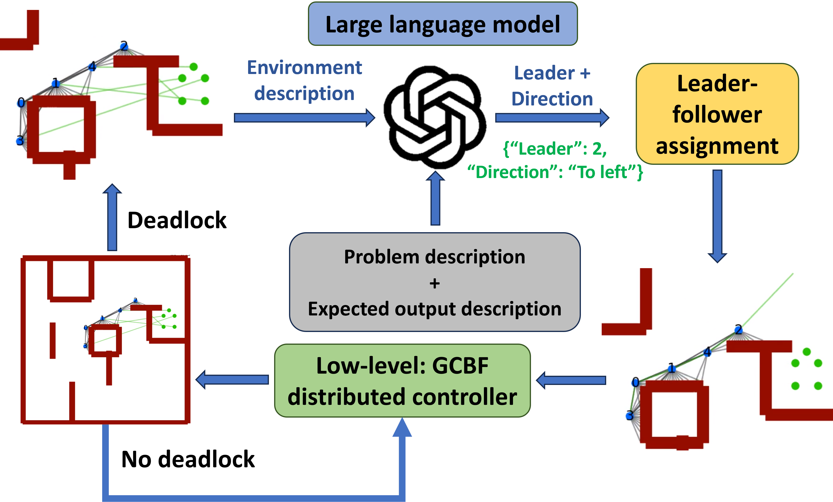
This work is motivated by the recent success of LLMs in assisting a control framework for complex robotics problems. While the aforementioned methods proactively use LLMs, whether directly for planning, translation, or reward design, we are instead interested in using LLMs reactively to resolve a class of failure modes in low-level controllers for MRS, namely deadlocks. This also helps ensure that the LLM cannot lead to a violation of safety as that is taken care of by the provably safe low-level control policy. When a deadlock is detected, we prompt an LLM to decide on a leader and a direction for that leader conditioned on a text-based description of the local observable environment and the state of the MRS. This temporary high-level assignment aims to move the MRS out of the deadlock to allow the low-level controller to continue making progress toward the goal.

Contributions  The contributions of the paper are two-fold. First, we extend the GCBF+ framework from [13] to also incorporate connectivity requirements. The GCBF+ framework uses a graph neural network (GNN) to learn a distributed control policy for collision avoidance, where the edge features encode the information essential for maintaining safety (i.e., relative state information). In this work, we append the edge features with the required connectivity information and modify the definition of the safe set to include connectivity requirements. Second, we utilize GPT3.5 from OpenAI via OpenAI Python API as the high-level planner. To the best of our knowledge, this is the first work that utilizes LLMs with the current environment information to assign a leader for MRS to resolve deadlocks. We prompt the LLM with a description of the problem setup and the observable environment information when the MRS gets stuck in a deadlock. We compare the performance of GPT3.5 when using various few-shot in-context examples. Our results demonstrate that LLM-based high-level planners are effective at resolving deadlocks in MRS. Based on our observations, we provide extensive discussion and possible future directions to improve the performance of LLMs as high-level planners for assisting low-level controllers in complex MRS problems.

II Problem formulation

In this work, we design a distributed control framework for large-scale robotic systems with multiple objectives. First, we start with describing the dynamics of the individual robots (referred to as agents henceforth), and then, we list the individual as well as the team objective for the system. The agent dynamics are given by $\dot{x}_{i}=f(x_{i})+g(x_{i})u_{i}$, where $f,g$ are locally Lipschitz continuous functions with $x_{i}\in\mathcal{X}\subset\mathbb{R}^{n_{x}}$ denoting agents’ state space and $u_{i}\in\mathcal{U}\subset\mathbb{R}^{n_{u}}$ the control constraint set for $i\in\{1,2,\dots,N\}$. The state $x_{i}$ consists of the position $p_{i}\in\mathbb{R}^{2}$ in the global coordinates along with other states, such as the orientation and the velocity of the agent $i$.

The state space $\mathcal{X}$ consists of stationary obstacles $\mathcal{O}_{l}\subset\mathbb{R}^{2}$ for $l\in\{1,2,\dots,M\}$, denoting walls, blockades and other obstacles in the path of the moving agents. Each agent has a limited sensing radius $R>0$ and the agents can only sense other agents or obstacles if it lies inside its sensing radius. The agents use LiDAR to sense the obstacles, and the observation data for each agent consists of $n_{\mathrm{rays}}$ evenly-spaced LiDAR rays originating from each robot and measures the relative location of obstacles. We denote the $j$-th ray from agent $i$ by $y_{j}^{(i)}\in\mathcal{X}$ for $j\in\{1,2,\dots,n_{\mathrm{rays}}\}$ that carries the relative position information of the $j-$th LiDAR hitting point to agent $i$, and zero padding for the rest of the states.

The time-varying connectivity graph $\mathcal{G}(t)=(\mathcal{V}(t),\mathcal{E}(t))$ dictates the network among the agents and obstacles. Here, $\mathcal{V}(t)=\mathcal{V}^{a}\cup\mathcal{V}^{o}(t)$ denotes the set of nodes, where $\mathcal{V}^{a}=\{1,2,\dots,N\}$ denotes the set of agents, $\mathcal{V}^{o}(t)$ is the collection of all LiDAR hitting points at time $t\geq 0$, and $\mathcal{E}(t)\subset\mathcal{V}^{a}\times\mathcal{V}$ denotes the set of edges, where $(i,j)\in\mathcal{E}(t)$ means the flow of information from node $j$ to agent $i$. We denote the time-varying adjacency matrix for agents by $A(t)\in\mathbb{R}^{N\times N}$, where $A_{ij}(t)=1$ if $(i,j)\in\mathcal{E}(t),i,j\in\mathcal{V}^{a}$, and $0$ otherwise. The set of all neighbors for agent $i$ is denoted as $\mathcal{N}_{i}(t)\coloneqq\{j\;|\;(i,j)\in\mathcal{E}(t)\}$, while the set of agent neighbors of agent $i$ is denoted as $\mathcal{N}_{i}^{a}(t)\coloneqq\{j\;|\;A_{ij}(t)=1\}$. The MRS is said to be connected at time $t$ if there is a path between each pair of agents $(i,j),i,j\in\mathcal{V}^{a}$ at $t$. One method of checking the connectivity of the MRS is through the Laplacian matrix, defined as $L(A(t))\coloneqq D(t)-A(t)$, where $D(t)$ is the degree matrix defined as $D_{ij}(t)=\sum\limits_{j}A_{ij}(t)$ when $i=j$ and $0$ otherwise. From [35, Theorem 2.8], the MRS is connected at time $t$ if and only if the second smallest eigenvalue of the Laplacian matrix is positive, i.e., $\lambda_{2}(L(A(t)))>0$. Now we have all the elements to introduce the problem statement.

Problem 1.

Consider the multi-agent system with initial conditions $\{x_{i}(0)\}_{i=1}^{N}$ such that the underlying graph $\mathcal{G}(0)$ is connected, safety parameters $r>0$, a sensing radius $R>0$, a set of stationary obstacles $\{\mathcal{O}_{j}\}_{j=1}^{M}$, and goal locations $\{p^{\mathrm{goal}}_{i}\}_{i=1}^{N}$. Design a control policy $\pi_{i}$ using information available in agent $i$’s sensing radius, such that

• Safety: The agent maintains a safe distance from other agents and obstacles at all times, i.e., $\|p_{i}(t)-p_{j}(t)\|\geq 2r,\forall j\neq i$ and $\|y^{(i)}_{j}(t)\|>r,\;\forall j=1,\dots,n_{\mathrm{rays}}$ for all $t\geq 0$;

• Connectivity: The graph $\mathcal{G}(t)$ remains connected at all times, i.e., $\lambda_{2}(L(A(t)))>0$ for all $t\geq 0$;

• Performance: The agents reach their respective goal locations, i.e., $\lim\limits_{t\to\infty}\|p_{i}(t)-p^{\mathrm{goal}}_{i}\|=0$.

Figure 2: Illustration of leader assignment for evading deadlock situation due to presence of an obstacle. The "Star" markers denote the goal locations, while the circular object is an obstacle. The connectivity of the MRS prevents the agents from going around the obstacle to reach their goal under the low-level control policy.

III Hierarchical control architecture

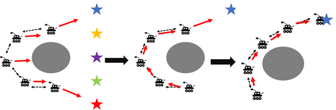
In a multi-agent motion planning problem without a high-level planner, the presence of obstacles can lead to deadlock situations as illustrated in the first image of Figure 2. Here, the agents at the end of the network chain try to go directly toward their respective goal locations while trying to maintain connectivity as well. Such situations can be evaded by assigning a temporary goal location via leader assignment where the assigned leader acts as temporary goal $\bar{p}^{\mathrm{goal}}_{i}$ for agent $i$. In a simple scenario consisting of a small number of agents and obstacles such as the one illustrated in Figure 2 with just 5 agents and 1 obstacle, it is possible to assign the leader manually. However, for more complex scenarios consisting of multiple obstacles, it is not straightforward how to effectively choose a leader. In this work, we use an LLM for leader assignment based on the current information available to the MRS. First, we describe the criteria to query an LLM for such an intervention.

Criteria for intervention  We use a leader-based goal assignment to resolve a deadlock due to the presence of obstacles. This assignment is triggered when the average speed of the MRS falls below a minimum threshold $\delta_{v}>0$, i.e., $\frac{\sum_{i}\|\dot{p}_{i}\|}{N}<\delta_{v}$ and the average distance of the agents from their goals is at least $\delta_{d}>0$, i.e., $\frac{\sum_{i}\|p_{i}-p^{\mathrm{goal}}_{i}\|}{N}>\delta_{d}$. These criteria imply that the MRS is stuck in a deadlock due to the obstacles as the agents are not near the desired goals. Since the graph topology is connected, the average speed (which requires global information) can be computed through consensus updates.

Leader-follower formation The high-level planner (i.e., the LLM) assigns a leader among the $N$ agents. In addition, a direction of motion for the leader is also required since the obstacle may occlude the leader’s path toward its goal, resulting in the leader getting stuck in a deadlock. Once a leader is assigned, the follower assignment is carried out in an iterative way. Let $\mathcal{V}_{\mathrm{lead}}(t,k)$ be the set of agents that have been assigned as a leader at time $t$, iteration $k$, initiated as $\mathcal{V}_{\mathrm{lead}}(t,0)=\{i_{\mathrm{lead},0}\}$, where $i_{\mathrm{lead},0}\in\mathcal{V}$ is the leader agent. Then, the $k-$th follower with $k\geq 1$ is chosen as

$$i_{\mathrm{follow},k}=\operatorname*{arg\min}_{j\in\mathcal{V}\setminus\mathcal{V}_{\mathrm{lead}}(t,k-1)}\min_{i\in\mathcal{V}_{\mathrm{lead}}(t,k-1)}\|p_{i}-p_{j}\|,$$ (1)

and this follower is added to the set of the leaders, i.e., $\mathcal{V}_{\mathrm{lead}}(t,k)=\mathcal{V}_{\mathrm{lead}}(t,k-1)\cup\{i_{\mathrm{follow},k}\}$. The leader for the $k-$th follower is given as $i_{\mathrm{lead},k}=\operatorname*{arg\min}\limits_{i\in\mathcal{V}_{\mathrm{lead}}(t,k-1)}\|p_{i_{\mathrm{follow},k}}-p_{i}\|$. The process is repeated till each agent $i$ is assigned an agent $i_{\mathrm{lead}}$ to follow. Next, for each agent $i$ that is a given minimum distance away from its goal, their temporary goal is chosen as the location of their leaders, i.e., $\bar{p}^{\mathrm{goal}}_{i}=p_{i_{\mathrm{lead}}}$.

IV LLM for leader assignment

To initiate the follower assignment process, it is necessary to designate a leader and assign it a direction. The choice of leader and direction depends on the state of the MRS, such as the configuration of agents, and the local observations of the surrounding environment. We use an LLM to perform this designation and assignment.

IV-A Prompt design

In order to use a pre-trained LLM for the novel task of leader assignment, we provide the LLM with task-relevant context that is expected to be helpful when generating a decision. In particular, the prompt to the model consists of three main components: (1) the Task description, (2) an Environment state, and (3) the Desired output. We also optionally include In-context examples to investigate other prompting techniques. The final design of the prompt is a result of iterating over several possible designs applied to a small set of deadlock problems; we do not claim that our prompt is optimal for this task. Below we explain each of the prompt components in more detail.

Task description  The initial part of the prompt consists of a description of the deadlock resolution problem for a multi-robot system. This includes the system requirements of maintaining safety, connectivity, and each agent reaching its assigned goal. Further, we include a description of the LLM’s role in providing high-level commands when the MRS is stuck in a deadlock. This component of the prompt is created offline and is fixed during roll-out.

Environment state  The state of the environment and the MRS is a necessary context for making a good leader assignment decision, so we encode it in a textual description that is included as a component of the prompt. Since the environment state depends on the roll-out of the system, we construct this part of the prompt online after a deadlock has been detected. Specifically, at any given time instant $t_{q}$ when the LLM is queried, the environment state is represented as the following tuple: (Number of agents, Safety radius, Connectivity radius, Agent locations, Agent goals, Locations of visible obstacles), where the agent locations are $\{p_{i}(t_{q})\}$, the goals $\{p^{\mathrm{goal}}_{i}\}$, visible obstacles $\{o_{i}(t_{q})\}$ whose information comes from the LiDAR data (see Section V for more details) and the connections from the adjacency matrix $A(t_{q})$. Note that we do not assume that the complete state-space information is available to the MRS and only provide the information currently available to the MRS, i.e., the currently visible obstacles.

Desired output  Finally, we provide a description of the desired output, both in terms of content and format. The LLM is responsible for choosing a leader and direction. To help constrain the model’s output and enable consistent output parsing, we request the generated response to be formatted as a JSON object with fields for “Leader" and “Direction"; the OpenAI API provides a JSON response mode that makes such output formatting reliable. The fields for “Leader" and “Direction" expect integer values from $\{1,2,\dots,n\}$ and elements from the set {“To left", “To right", “To goal"}, respectively. The rationale behind using these values for the direction is twofold: a) it keeps the space of the desired LLM outputs small (i.e., 3); and b) at least one of these three directions will lead to deadlock resolution with the correct choice of the leader. We conclude with suggestions about good leader assignment, namely that it should minimize the traveling distance of agents toward their goals and that a good direction for the assigned leader should depend on the impact of near obstacles on the leader’s ability to move.

In-context examples  In some variations of our approach, we optionally also include $k$ in-context examples of good leader assignment for different instances of a system in deadlock, where $k$ is set a priori. Each example consists of the textual environment state description for the deadlock, as previously described, and the corresponding JSON-formatted output with the chosen leader and direction. To provide examples of good leader assignments, we sample from leader assignments in trials that had good overall task performance (i.e. all agents reached their goals). The examples for in-context learning are taken from deadlock instances encountered during the $0-$shot runs with an LLM as a high-level planner. To discourage the LLM from merely repeating the leader assignments in the examples, we choose examples with some diversity over the number of agents, the chosen direction, and the ID of the selected leader. The exact prompts used in the experiments are provided on the project website.

V Distributed low-level policy

The high-level planner provides the leader and the goal information to the controller at the low level. One desirable property of the low-level controller is scalability and generalizability to new environments (i.e., changing the number of agents and obstacles) while having safety guarantees. To this end, we use the GCBF-based distributed control framework from [13] to design the low-level control policy. The low-level controller synthesizes an input $u_{i}$ to maintain the connectivity, keep the system safe from obstacles and other agents, and drive the system trajectories toward its goal location. For the sake of completeness, we briefly describe the notion of GCBF and the GNN-based training framework, termed GCBF+, in [13] below.

V-A GCBF+ for safety

Given sensing radius $R$ and safety distance $r$, define $N_{s}-1\in\mathbb{N}$ as the maximum number of neighbors that each agent can have while all the agents in the neighborhood remain safe. Define $\tilde{\mathcal{N}}_{i}$ as the set of $N_{s}$ closest neighboring nodes to agent $i$ which also includes agent $i$ and $\bar{x}_{\tilde{\mathcal{N}}_{i}}$ as the concatenated vector of $x_{i}$ and the neighbor node states with fixed size $N_{s}$ that is padded with a constant vector if $|\tilde{\mathcal{N}_{i}}|<N_{s}$. Considering only collision avoidance constraints, the safe set $\mathcal{S}_{N}\in\mathcal{X}^{N}$ can be defined as:

$$\mathcal{S}_{N}\coloneqq\Big{\{}\bar{x}\in\mathcal{X}^{N}\;\Big{|} \;\Big{(}\left\lVert y_{j}^{(i)}\right\rVert>r,\;\forall i\in\mathcal{V}^{a},\forall j\in n_{\mathrm{rays}}\Big{)}\bigwedge$$

$$\Big{(}\min_{i,j\in\mathcal{V}_{a},i\neq j}\left\lVert p_{i}-p_{j}\right\rVert>2r\Big{)}\Big{\}}.$$

The unsafe, or avoid set can be defined accordingly as $\mathcal{A}_{N}=\mathcal{X}^{N}\setminus\mathcal{S}_{N}$. Before introducing the notion of graph CBF for MRS, we review the notion of CBF traditionally used for single-robot system. Consider a system $\dot{x}=F(x,u)$ where $x\in\mathcal{X}\subset\mathbb{R}^{n_{x}}$, $u\in\mathcal{U}\subset\mathbb{R}^{n_{u}}$ and $F:\mathbb{R}^{n_{x}}\times\mathbb{R}^{n_{u}}\to\mathbb{R}^{n_{x}}$. Let $\mathcal{C}\subset\mathcal{X}$ be the $0$-superlevel set of a continuously differentiable function $h:\mathcal{X}\rightarrow\mathbb{R}$, i.e., $\mathcal{C}=\{x\in\mathcal{X}:h(x)\geq 0\}$. Then, $h$ is a CBF if there exists an extended class-$\mathcal{K}$ function $\alpha:\mathbb{R}\rightarrow\mathbb{R}$ such that:

$$\sup_{u\in\mathcal{U}}\left[\frac{\partial h}{\partial x}F(x,u)+\alpha\left(h(x)\right)\right]\geq 0,\quad\forall x\in\mathcal{X}.$$ (2)

Let $\mathcal{S}\subset\mathcal{X}$ denote a safe set with the objective that the system trajectories do not leave this set. If $\mathcal{C}\subset\mathcal{S}$, then the existence of a CBF implies the existence of a control input $u$ that keeps the system safe [8]. Next, we review the notion of GCBF from [13].

Definition 1 (GCBF).

A continuously differentiable function $h:\mathcal{X}^{N_{s}}\rightarrow\mathbb{R}$ is a Graph CBF (GCBF) if there exists an extended class-$\mathcal{K}$ function $\alpha$ and a control policy $\pi_{i}:\mathcal{X}^{N_{s}}\rightarrow\mathcal{U}$ for each agent $i\in\mathcal{V}_{a}$, such that $\dot{h}(\bar{z}_{\tilde{\mathcal{N}}_{i}})+\alpha(h(\bar{z}_{\tilde{\mathcal{N}}_{i}}))\geq 0,\quad\forall i\in\mathcal{V}_{a}$ for all $\bar{z}\in\mathcal{X}^{N}$ with $N>N_{s}$ where $\dot{h}(\bar{z}_{\tilde{\mathcal{N}}_{i}})=\sum_{j\in\tilde{\mathcal{N}}_{i}}\frac{\partial h(\bar{x}_{\tilde{\mathcal{N}}_{i}})}{\partial x_{i}}(f(x_{j})+g(x_{j})u_{j})$, for $u_{j}=\pi_{j}(\bar{x}_{\tilde{\mathcal{N}}_{i}})$.

Following [13], we use graph neural networks (GNN) to parameterize GCBF. For agent $i$, the input features of the GNN contains the node features $v_{i},v_{j},j\in\mathcal{N}_{i}$, and edge features $e_{ij},j\in\mathcal{N}_{i}$. The design of the node features and edge features is the same as [13] except for adding connectivity information in the edge features as explained below.

V-B Connectivity constraint in GCBF+

In addition to the safety constraint incorporated in the GCBF+ framework [13] as described above, we also need to account for the connectivity requirement of Problem 1. To this end, given the desired connectivity of the MRS in terms of the desired adjacency matrix $A^{d}$ where the desired adjacency matrix is designed such that the MRS is connected, we add the connectivity information in the edge features of GCBF. In particular, we append the edge features with $[0,1]^{\top}$ in $e_{ij}$ if the agents $(i,j)$ are required to be connected, i.e., $A^{d}_{ij}=1$, and $[1,0]^{\top}$ if they are not required to be connected, i.e., if $A^{d}_{ij}=0$. Furthermore, we add the connectivity constraint in the GCBF by redefining the safe and the unsafe sets corresponding to the required connectivity. We modify the collision-avoidance safety to account for connectivity constraints as

$$\mathcal{S}_{N}^{c}\coloneqq\Big{\{}\bar{x}\in\mathcal{X}^{N}\;\Big{|} \;\Big{(}\left\lVert y_{j}^{(i)}\right\rVert>r,\;\forall i\in\mathcal{V}_{a},\forall j\in n_{\mathrm{rays}}\Big{)}\bigwedge$$

$$\Big{(}\min_{i,j\in\mathcal{V}_{a},i\neq j}\left\lVert p_{i}-p_{j}\right\rVert>2r\Big{)}\bigwedge$$

$$\Big{(}\max_{i,j\in\mathcal{V}_{a},A^{d}_{ij}=1}\left\lVert p_{i}-p_{j}\right\rVert<R\Big{)}\Big{\}}$$

Consequently, the unsafe set with the connectivity constraint is defined as $\mathcal{A}^{c}_{N}=\mathcal{X}^{N}\setminus\mathcal{S}^{c}_{N}$. For a GCBF $h$, let $\mathcal{C}_{h}^{c}\in\mathcal{X}^{N_{s}}$ denote the $0$-superlevel set of $h$

$$\mathcal{C}_{h}^{c}\coloneqq\{\tilde{x}\in\mathcal{X}^{N_{s}}|h(\tilde{x})\geq 0\},$$ (3)

and define $\mathcal{C}_{N}^{c}\in\mathcal{X}^{N}$ as the set of $N$-agent states where $\bar{x}_{\tilde{\mathcal{N}}_{i}}$ lie inside $\mathcal{C}_{h}^{c}$ for all $i\in\mathcal{V}_{a}$. Then following [13, Theorem 1], we have the following proposition.

Proposition 1.

Suppose $h$ is a GCBF, and for any given agent $i\in\mathcal{V}_{a}$, a neighboring node $j$ such that $\|p_{i}-p_{j}\|\geq R$ does not affect the GCBF $h$. Suppose $\mathcal{C}_{N}^{c}\subset\mathcal{S}_{N}^{c}$ for each $N\in\mathbb{N}$. Then, for any $N\in\mathbb{N}$, the resulting closed-loop trajectories of the MAS with initial conditions $\bar{x}(0)\in\mathcal{C}_{N}^{c}$ satisfy $\bar{x}(t)\in\mathcal{S}_{N}^{c}$ for all $t\geq 0$, under any locally Lipschitz continuous control input $\bar{u}:\mathcal{X}^{N}\rightarrow\mathcal{U}_{s}^{N}$, where

$$\mathcal{U}_{s}^{N}\coloneqq\Big{\{}\bar{u}\in\mathcal{U}^{N}\Big{|}\dot{h}(\bar{x}_{\tilde{\mathcal{N}}_{i}})+\alpha(h(\bar{x}_{\tilde{\mathcal{N}}_{i}}))\geq 0,\forall i\in\mathcal{V}_{a}\Big{\}}.$$ (4)

Learning GCBF and distributed control  The training framework is the same as [13]. In the original GCBF+ training framework, it is essential that the initial and goal locations are safe. In the current work, we also need to make sure that the initial conditions and the goal locations sampled for training the GCBF satisfy the MRS connectivity condition, in addition to the safety condition in the original GCBF+ framework. To this end, we sample the initial and goal locations such that their corresponding graph topology are connected, and define the desired adjacency matrix $A^{d}=A(0)$. In the interest of space, we omit the details of the loss function design and obtain training data; interested readers are referred to [13].

VI Evaluations

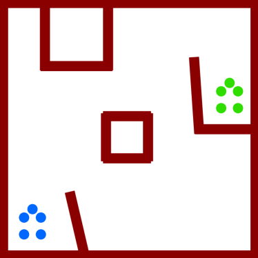
We perform experiments on two sets of environments, namely a highly structured hand-crafted environment (termed henceforth as "Room environment", or simply, "Room") and randomly generated environments (termed henceforth "Random environment", or simply "Random"). The structured room environment as well as an instance of a randomized room environment are depicted in Figure 3.

Figure 3: Illustration of the “Room" environment (left) and the randomized environment right. Here, the agents are shown in the blue color, their goals in green, and the obstacles in red color.

The test objectives are described below:

• How effective is the LLM at providing a high-level command that can help each agent reach their respective goal locations?

• What is the impact of in-context examples on the rate of completion when using an LLM-based high-level planner?

We report the number of agents reaching their goals and the total number of times the high-level planner intervenes.

VI-A Test environments

“Room" environments: The “Room" represents an enclosed warehouse or an apartment scenario where the agents are required to reach another part of the environment while remaining inside the boundary and avoiding collisions with walls and other obstacles in the room. The agents start in one corner of the room and propagate their way through the obstacle environment to reach their respective destinations. The obstacles and the walls in the room environment are designed in such a manner that the underlying GCBF+ control policy invariably gets stuck in a deadlock, making it essential to use a high-level planner (see Figure 4). Here, we generate a variety of such environments where the angles, lengths, and locations of the walls are randomized.

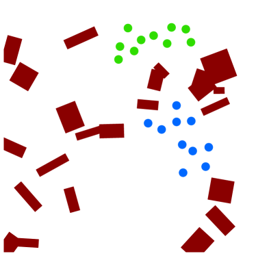
“Random" environment  The “Random" environment consists of randomly generated $n$ initial and goal locations such that the underlying graph topology defined on the set of initial and goal locations are connected. In addition, it has $M$ randomly generated rectangular obstacles of randomly generated sizes and orientations. For testing, we use $n=\{5,10,15\}$ and $M=\{25,40\}$, and in total, we generate 24 of such randomly generated environments for experiments.

VI-B Baselines

We use just the low-level controller without any leader assignment and a hand-designed heuristic high-level planner as the baselines. The heuristic leader assignment policy chooses the leader based on a combination of the distance of an agent to its goal and how fast the MRS will move with that agent being the leader.

LLMs used for testing  We use GPT3.5 as the candidate for high-level planners for the MRS. We evaluate the performance of GPT3.5-$k$ with $k\in\{0,1,5,10,15\}$ for $k$ in-context examples used in the prompts. The response generated by an LLM depends on how each generated token is sampled from the inferred token distribution, which can be tuned according to a temperature parameter in the OpenAI API. In most cases, we set the temperature to 0, which essentially enforces that the sampled token is always the most likely. We also investigate the performance of using non-deterministic results. To this end, we set the temperature parameter to 1.0 and query the LLM with the same prompt 10 times. The most frequent response is taken as the final output to be used for the leader assignment. The result of this ensemble-based setup is reported with the label GPT3.5-Ens.

Figure 4: Frequency (left axis) of trials in which N agents reach their goal for 20 instances of the Randomized Room environment (shown in thin colored bars), and the average number of agents reaching their goal per trial (right axis) for each tested high-level planner (shown in the thick gray bar).

Figure 5: Number of interventions for each high-level planner. The “No leader" method has exactly zero interventions as it does not use any high-level planner.

Figure 6: Mean and standard deviation for the number of agents reaching their goal for the random environments with 25 and 40 obstacles for N agents, where N is {5, 10, 15}.

Figure 7: Number of interventions for each high-level planner. The “No leader" method has exactly zero interventions as it does not use any high-level planner.

VI-C Roll-out for evaluation

To evaluate the effectiveness of the high-level planner, we roll out MRS trajectories for a fixed number of steps $T=2500$. As mentioned earlier, the high-level planner intervenes when the MRS gets stuck in a deadlock which is defined based on the minimum average speed criteria. In this work, we use $\delta_{v}=0.2$ and $\delta_{d}=0.4$ as the threshold for defining deadlocks. Once the high-level planner assigns a leader, the MRS stays in the same leader-follower configuration for $20$ steps. This is useful as it helps prevent Zeno behaviors. This also sets an upper bound on the frequency at which the LLM is queried and makes the LLM-in-the-loop control framework real-time.

VI-D Results

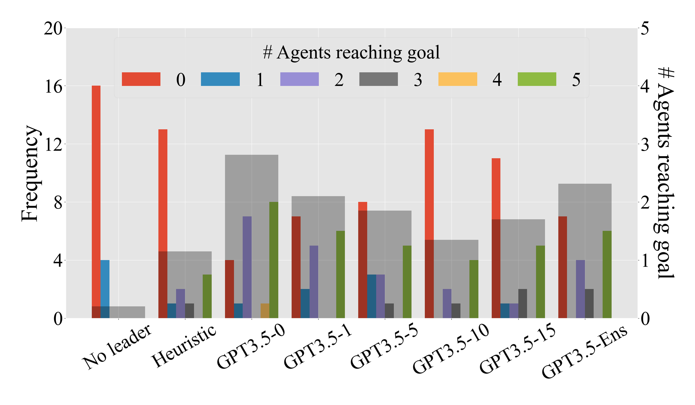
Figure 4 reports performance metrics for each high-level planner in the Randomized Room environment. The thin, colored bars show the frequency of trials for which N out of 5 agents reached their goal over 20 trials; these bars correspond to the left y-axis. The thick, gray bars show the average number of agents that reached their goal over the same 20 trials; these bars correspond to the right y-axis. The baseline with no high-level planner (“no leader") performs the worst with the most trials in which no agents reached their goal and no trials in which all agents reached their goal. The hand-designed heuristic planner had three trials with all agents reaching their goal but has the second worst performance of all methods. The LLM-based planners all outperformed the baselines with fewer instances of zero goal-reaching agents. Of these, GPT3.5 with zero in-context examples performed best. Performance consistently decreased for increasing numbers of in-context examples, with more instances of no goal-reaching agents and fewer trials with five goal-reaching agents. The non-deterministic LLM-based planner (GPT3.5-Ens) performed worse than its deterministic counterpart (GPT3.5-0).

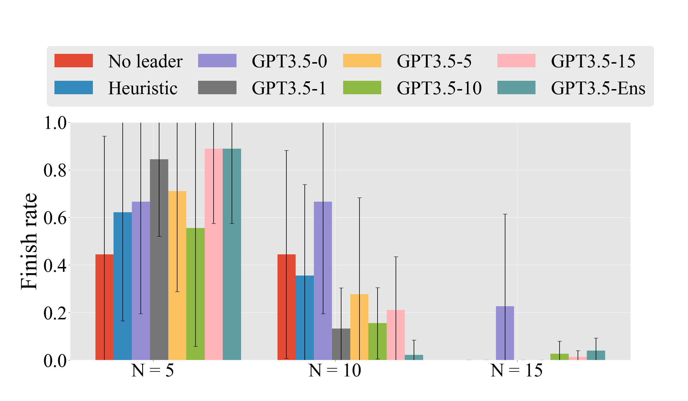
Figure 6 reports the average number of goal-reaching agents for each high-level planner in the Random environments. It shows that for the scenarios with five agents, the heuristic planner performs better than no high-level planner, although the performance drops for teams of ten agents. The LLM-based planners have mixed results. Taking the most frequent response of the ten sampled responses (GPT3.5-Ens) performs best in the five-agent scenario, resulting in all agents reaching their goal for most cases; however, it performs the worst in the ten-agent scenario, failing to get any goal-reaching agents for almost all cases. For deterministic LLM-based planners using $k$ in-context examples, we find that $k=15$ performs the best for five agent scenarios and $k=0$ performs the best for ten agent teams. While some non-zero $k$ values perform well for five agents, these all significantly drop in performance for ten agents. For the 15-agent scenario, most planners fail in almost all cases, with only $k=0$ exhibiting any notable success, implying that deadlock resolution in such cases is prohibitively challenging for all tested planners.

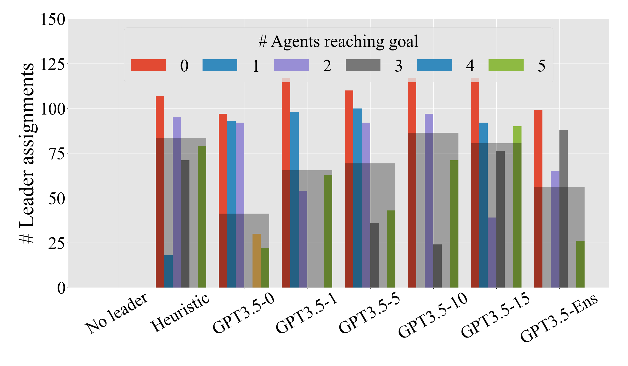
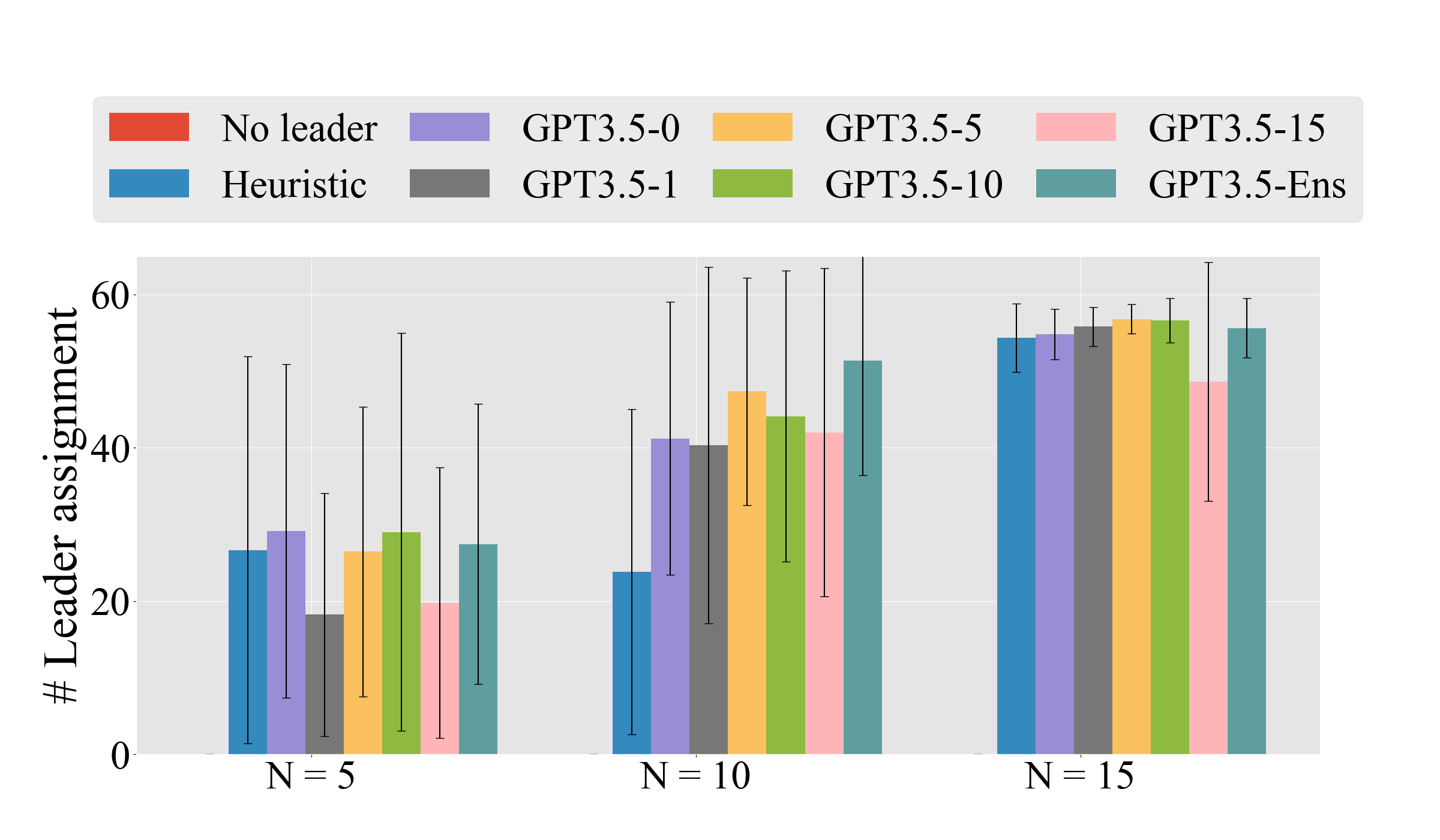
Figures 5 & 7 report the average number of times the high-level planner intervened in the Random and Random Room environments, respectively. Intuitively, fewer interventions should roughly correlate with higher quality decisions per intervention, and this is supported by comparing the performance results in Figures 4 & 6 with the frequencies of interventions in Figures 5 & 7, respectively. These results imply that the LLM-based planners are often producing higher quality decisions when intervening, further supporting the claim that they are promising as high-level planners for deadlock resolution.

VII Discussion and Conclusions

In general, the results in Figures 4 & 6 show that LLM-based planners can significantly outperform the reported baselines. The relative performance improvement is greatest for five agent teams as seen in both the Randomized Room and the Random environments. While the results for the LLM-based planners are mixed for the ten-agent scenario, we find that using zero in-context examples still significantly outperforms the baselines. This is good evidence that LLMs are promising as high-level planners for deadlock resolution.

The non-deterministic LLM-based planner (GPT3.5-Ens) has a very large drop in performance from the five-agent scenario to the ten-agent scenario. Upon inspection, we observed that the most frequent response in the five-agent scenario was typically much more frequent than the other responses, whereas the most frequent response in the ten-agent scenario typically occurred only slightly more frequently than other responses. We hypothesize that this is a result of there being more possible leader assignments as the number of agents increases. Increasing the number of samples could help improve performance for scenarios with more agents.

After the high-level planner intervenes and the temporary goal direction is replaced with the original goals, the system may return to the same deadlock state and require another intervention. As a rough measure of intervention quality, a better intervention is one that avoids the system returning to the same deadlock, and such repetition would result in more interventions over a full roll-out. We are encouraged that, in many cases, the LLM-based planners need to intervene less frequently, implying better intervention quality.

The results also show that LLM-based planner performance is sensitive to the in-context examples. We tested different ways of selecting the in-context examples to use, such as randomly selecting from a curated set of examples with varying numbers of agents or only selecting examples with the same number of agents as the deadlock to be resolved. However, we did not observe clear performance improvements with any specific choice. Surprisingly, for the Randomized Room environment, in-context examples generally decreased performance. There are many possible ways to structure and choose the in-context examples, such as using language model embeddings to identify and choose the in-context examples that are most similar to the current deadlock, and we are interested in exploring further. We are also interested in exploring other prompt techniques, such as chain-of-thought [16], that have been shown to produce better results on some tasks.

More generally, the prompt design used in this work is the result of manual trial and error while following generally accepted practices for prompt engineering. Recently, there is interest in automatic prompt optimization for black-box LLMs to find the best prompt design for a given task [36, 37, 38] with results showing significant performance improvement over human-designed prompts. Future work includes applying such techniques to the problem of deadlock resolution to maximize the performance of LLMs as a high-level planner.

One trade-off of using an LLM as a high-level planner is the time it takes to query the model and receive a response. For real-time intervention, fast performance can often be a prerequisite. Future work involves investigating possible methods to improve the runtime, such as using smaller LLMs finetuned to the specific task or using embedding models that can capture semantic context with significantly lower runtime.

In this work, the high-level planner intervenes according to a heuristic threshold of average agent velocity. We are interested in better anticipating and detecting deadlock states for two reasons. First, in some cases, the detected deadlock is not a true deadlock in the sense that, given enough time, a local controller might eventually escape, so intervention may not be necessary. Second, if the system can better anticipate deadlocks, the high-level planner can intervene earlier. Future work includes using embeddings of the local environment information, whether as text or potentially images, as a way to classify whether a deadlock is likely to occur.

References

- [1] B. Li and H. Ma, “Double-deck multi-agent pickup and delivery: Multi-robot rearrangement in large-scale warehouses,” IEEE Robotics and Automation Letters, vol. 8, no. 6, pp. 3701–3708, 2023.
- [2] P. R. Wurman, R. D’Andrea, and M. Mountz, “Coordinating hundreds of cooperative, autonomous vehicles in warehouses,” AI magazine, vol. 29, no. 1, pp. 9–9, 2008.
- [3] J. Dinneweth, A. Boubezoul, R. Mandiau, and S. Espié, “Multi-agent reinforcement learning for autonomous vehicles: a survey,” Autonomous Intelligent Systems, vol. 2, no. 1, p. 27, 2022.
- [4] Y. Tian, K. Liu, K. Ok, L. Tran, D. Allen, N. Roy, and J. P. How, “Search and rescue under the forest canopy using multiple uavs,” The International Journal of Robotics Research, vol. 39, no. 10-11, pp. 1201–1221, 2020.
- [5] J. Cortes, S. Martinez, T. Karatas, and F. Bullo, “Coverage control for mobile sensing networks,” IEEE Transactions on robotics and Automation, vol. 20, no. 2, pp. 243–255, 2004.
- [6] F. Mehdifar, C. P. Bechlioulis, F. Hashemzadeh, and M. Baradarannia, “Prescribed performance distance-based formation control of multi-agent systems,” Automatica, vol. 119, p. 109086, 2020.
- [7] A. D. Ames, S. Coogan, M. Egerstedt, G. Notomista, K. Sreenath, and P. Tabuada, “Control barrier functions: Theory and applications,” in 2019 18th European control conference (ECC). IEEE, 2019, pp. 3420–3431.
- [8] A. D. Ames, X. Xu, J. W. Grizzle, and P. Tabuada, “Control barrier function based quadratic programs for safety critical systems,” IEEE Transactions on Automatic Control, vol. 62, no. 8, pp. 3861–3876, 2017.
- [9] L. Wang, A. D. Ames, and M. Egerstedt, “Safety barrier certificates for collisions-free multirobot systems,” IEEE Transactions on Robotics, vol. 33, no. 3, pp. 661–674, 2017.
- [10] C. Dawson, S. Gao, and C. Fan, “Safe control with learned certificates: A survey of neural lyapunov, barrier, and contraction methods for robotics and control,” IEEE Transactions on Robotics, vol. 39, no. 3, pp. 1749–1767, 2023.
- [11] S. Zhang, K. Garg, and C. Fan, “Neural graph control barrier functions guided distributed collision-avoidance multi-agent control,” in 7th Annual Conference on Robot Learning, 2023.
- [12] K. Garg, S. Zhang, O. So, C. Dawson, and C. Fan, “Learning safe control for multi-robot systems: Methods, verification, and open challenges,” Annual Reviews in Control, vol. 57, p. 100948, 2024.
- [13] S. Zhang, O. So, K. Garg, and C. Fan, “Gcbf+: A neural graph control barrier function framework for distributed safe multi-agent control,” arXiv preprint arXiv:2401.14554, 2024.
- [14] T. Brown, B. Mann, N. Ryder, M. Subbiah, J. D. Kaplan, P. Dhariwal, A. Neelakantan, P. Shyam, G. Sastry, A. Askell et al., “Language models are few-shot learners,” Advances in neural information processing systems, vol. 33, pp. 1877–1901, 2020.
- [15] T. Kojima, S. S. Gu, M. Reid, Y. Matsuo, and Y. Iwasawa, “Large language models are zero-shot reasoners,” in ICML 2022 Workshop on Knowledge Retrieval and Language Models, 2022. [Online]. Available: https://openreview.net/forum?id=6p3AuaHAFiN
- [16] J. Wei, X. Wang, D. Schuurmans, M. Bosma, F. Xia, E. Chi, Q. V. Le, D. Zhou et al., “Chain-of-thought prompting elicits reasoning in large language models,” Advances in Neural Information Processing Systems, vol. 35, pp. 24 824–24 837, 2022.
- [17] S. Yao, D. Yu, J. Zhao, I. Shafran, T. L. Griffiths, Y. Cao, and K. R. Narasimhan, “Tree of thoughts: Deliberate problem solving with large language models,” in Thirty-seventh Conference on Neural Information Processing Systems, vol. 36, 2024.
- [18] M. Besta, N. Blach, A. Kubicek, R. Gerstenberger, L. Gianinazzi, J. Gajda, T. Lehmann, M. Podstawski, H. Niewiadomski, P. Nyczyk et al., “Graph of thoughts: Solving elaborate problems with large language models,” arXiv preprint arXiv:2308.09687, 2023.
- [19] B. Wang, Z. Wang, X. Wang, Y. Cao, R. A Saurous, and Y. Kim, “Grammar prompting for domain-specific language generation with large language models,” Advances in Neural Information Processing Systems, vol. 36, 2024.
- [20] W. Huang, P. Abbeel, D. Pathak, and I. Mordatch, “Language models as zero-shot planners: Extracting actionable knowledge for embodied agents,” in International Conference on Machine Learning. PMLR, 2022, pp. 9118–9147.
- [21] A. Brohan, Y. Chebotar, C. Finn, K. Hausman, A. Herzog, D. Ho, J. Ibarz, A. Irpan, E. Jang, R. Julian et al., “Do as i can, not as i say: Grounding language in robotic affordances,” in Conference on robot learning. PMLR, 2023, pp. 287–318.
- [22] K. Lin, C. Agia, T. Migimatsu, M. Pavone, and J. Bohg, “Text2motion: From natural language instructions to feasible plans,” Autonomous Robots, vol. 47, no. 8, pp. 1345–1365, 2023.
- [23] W. Huang, F. Xia, T. Xiao, H. Chan, J. Liang, P. Florence, A. Zeng, J. Tompson, I. Mordatch, Y. Chebotar et al., “Inner monologue: Embodied reasoning through planning with language models,” in Conference on Robot Learning. PMLR, 2023, pp. 1769–1782.
- [24] Y. Chen, J. Arkin, Y. Zhang, N. Roy, and C. Fan, “Scalable multi-robot collaboration with large language models: Centralized or decentralized systems?” in International Conference on Robotics and Automation. IEEE, 2024.
- [25] ——, “Autotamp: Autoregressive task and motion planning with llms as translators and checkers,” in International Conference on Robotics and Automation, 2024.
- [26] Y. Chen, R. Gandhi, Y. Zhang, and C. Fan, “NL2TL: Transforming natural languages to temporal logics using large language models,” in Proceedings of the 2023 Conference on Empirical Methods in Natural Language Processing, 2023, p. 15880–15903.
- [27] Y. Xie, C. Yu, T. Zhu, J. Bai, Z. Gong, and H. Soh, “Translating natural language to planning goals with large-language models,” arXiv preprint arXiv:2302.05128, 2023.
- [28] T. Silver, V. Hariprasad, R. S. Shuttleworth, N. Kumar, T. Lozano-Pérez, and L. P. Kaelbling, “PDDL planning with pretrained large language models,” in NeurIPS 2022 Foundation Models for Decision Making Workshop, 2022. [Online]. Available: https://openreview.net/forum?id=1QMMUB4zfl
- [29] B. Liu, Y. Jiang, X. Zhang, Q. Liu, S. Zhang, J. Biswas, and P. Stone, “Llm+ p: Empowering large language models with optimal planning proficiency,” arXiv preprint arXiv:2304.11477, 2023.
- [30] I. Singh, V. Blukis, A. Mousavian, A. Goyal, D. Xu, J. Tremblay, D. Fox, J. Thomason, and A. Garg, “Progprompt: Generating situated robot task plans using large language models,” in 2023 IEEE International Conference on Robotics and Automation (ICRA). IEEE, 2023, pp. 11 523–11 530.
- [31] J. Liang, W. Huang, F. Xia, P. Xu, K. Hausman, B. Ichter, P. Florence, and A. Zeng, “Code as policies: Language model programs for embodied control,” in 2023 IEEE International Conference on Robotics and Automation (ICRA). IEEE, 2023, pp. 9493–9500.
- [32] W. Yu, N. Gileadi, C. Fu, S. Kirmani, K.-H. Lee, M. G. Arenas, H.-T. L. Chiang, T. Erez, L. Hasenclever, J. Humplik, brian ichter, T. Xiao, P. Xu, A. Zeng, T. Zhang, N. Heess, D. Sadigh, J. Tan, Y. Tassa, and F. Xia, “Language to rewards for robotic skill synthesis,” in 7th Annual Conference on Robot Learning, 2023.
- [33] T. Xie, S. Zhao, C. H. Wu, Y. Liu, Q. Luo, V. Zhong, Y. Yang, and T. Yu, “Text2reward: Dense reward generation with language models for reinforcement learning,” in The Twelfth International Conference on Learning Representations, 2024.
- [34] Y. J. Ma, W. Liang, G. Wang, D.-A. Huang, O. Bastani, D. Jayaraman, Y. Zhu, L. Fan, and A. Anandkumar, “Eureka: Human-level reward design via coding large language models,” in The Twelfth International Conference on Learning Representations, 2024.
- [35] M. Mesbahi and M. Egerstedt, “Graph theoretic methods in multiagent networks,” in Graph Theoretic Methods in Multiagent Networks. Princeton University Press, 2010.
- [36] Q. Guo, R. Wang, J. Guo, B. Li, K. Song, X. Tan, G. Liu, J. Bian, and Y. Yang, “Connecting large language models with evolutionary algorithms yields powerful prompt optimizers,” in The Twelfth International Conference on Learning Representations, 2024. [Online]. Available: https://openreview.net/forum?id=ZG3RaNIsO8
- [37] X. Wang, C. Li, Z. Wang, F. Bai, H. Luo, J. Zhang, N. Jojic, E. Xing, and Z. Hu, “Promptagent: Strategic planning with language models enables expert-level prompt optimization,” in The Twelfth International Conference on Learning Representations, 2024.
- [38] C. Fernando, D. Banarse, H. Michalewski, S. Osindero, and T. Rocktäschel, “Promptbreeder: Self-referential self-improvement via prompt evolution,” arXiv preprint arXiv:2309.16797, 2023.