Dynamic Deep Learning based Super-resolution for the Shallow Water Equations

Abstract

Using the nonlinear shallow water equations as benchmark, we demonstrate that a simulation with the ICON-O ocean model with a $20\text{\,}\mathrm{km}$ resolution that is frequently corrected by a U-net-type neural network can achieve discretization errors of a simulation with $10\text{\,}\mathrm{km}$ resolution. The network, originally developed for image-based super-resolution in post-processing, is trained to compute the difference between solutions on both meshes and is used to correct the coarse mesh every $12\text{\,}\mathrm{h}$. Our setup is the Galewsky test case, modeling transition of a barotropic instability into turbulent flow. We show that the ML-corrected coarse resolution run correctly maintains a balance flow and captures the transition to turbulence in line with the higher resolution simulation. After $8\text{\,}\mathrm{d}$ of simulation, the $L_{2}$-error of the corrected run is similar to a simulation run on the finer mesh. While mass is conserved in the corrected runs, we observe some spurious generation of kinetic energy.

65M99, 68T07, 86-08, 35-11

1 Introduction

Numerical models of the atmospheric and oceanic circulation greatly aid in our understanding of the climate [23] and are instrumental for numerical weather prediction (NWP). While there are fundamental differences regarding scales and driving forces between weather prediction and climate simulations, there are many similarities in the underlying equations and numerical techniques and several earth system models, like the Icosahedral Nonhydrostatic Model (ICON), are designed to be used for both. These models comprise two important components, the dynamical core and sub-grid models, so-called parameterizations. While the former is responsible for solving partial differential equations (PDEs) on the discrete grid, the latter is responsible for approximating the effect of processes such as diffusion, mixing, or turbulence that can not be resolved explicitly at a given spatio-temporal resolution [28]. To improve the accuracy of weather predictions and climate predictions and projections, there is a strong push towards ever finer grid resolutions [20]. However, finer mesh resolutions incur increasing computational cost and runtimes of climate models and energy consumption of HPC machines.

Machine Learning (ML) has been gaining popularity in many areas of simulation based science. ML techniques are applied in NWP and climate sciences in a manifold of different ways. Pure data-driven ML approaches, for example, are trained by reanalysis data that contain the optimal combination of model and observational information. These systems have started to challenge short and medium term weather predictions in terms of accuracy while being much more efficient [16, 22]. Physics-informed Machine-Learning aims to include physical relationships such as dynamical equations as a constraint within the optimization process [13]. ML techniques have also been applied to emulate unresolved physical processes such as convection, closures for eddy parametrizations of the ocean, or replacing specific subcomponents of the climate model [34, 35].

In recent years, the advent of super-resolution, a technique in machine learning, has significantly advanced the frontiers of image and video processing. Super-resolution endeavors to enhance the resolution of an image or video, aspiring to construct a high-resolution output from one or more low-resolution inputs [32]. This enhancement is used across a spectrum of applications, ranging from medical imaging and security surveillance to entertainment [4]. Central to super-resolution in machine learning is the deployment of deep convolutional neural networks [5] (CNNs) or Generative Adversarial Networks [17] (GANs) or Diffusion models [7]. These networks, through training on datasets comprising low-resolution and high-resolution image pairs, have demonstrated remarkable proficiency in generating high-resolution images from low-resolution inputs. A blend of super-resolution and image inpainting techniques has shown potential in enhancing outcomes, illustrating the synergy between these approaches. An example of this approach within climate science is the work of Kadow et al. 2020 [12], who apply image inpainting techniques, leveraging deep learning algorithms, to mitigate missing data issues in the HadCRUT4 temperature dataset. However, the utility of machine learning extends beyond the realms of image resolution enhancement and data gap mitigation and can help with bias correction in numerical climate models [19] or in other related [29] and non-related disciplines [33].

In our work, we integrate high-resolution information obtained by a neural network into a low-resolution configuration of the same model. Our approach augments a coarse, mesh-based algorithm by frequent modifications of the solution by the deep neural net, designed to improve the “effective resolution”, that is, correct the coarse solution towards the restriction of a solution computed on a finer mesh. Since this happens at runtime in the time-stepping loop, we call this approach “dynamic super-resolution”. We study if this hybrid system is capable of maintaining a balanced flow state and if it undergoes a transition to geostrophic turbulence similar to the high-resolution model. This is different from so-called “nudging-to-fine” approaches, that use ML to learn a state-dependent bias correction which is included in the source term of the governing PDE [2, 3]. A related hybrid ML-PDE solver was introduced by Pathak et al. for a two-dimensional turbulent flow simulation [21], but was based on the fine scale features of a quasi-steady solution, and thus cannot capture the transient behavior, e.g., the onset of instabilities. Our approach also shares some similarities with the recent work of Margenberg et al. [18]. In contrast to their architecture, our neural network is purely convolutional, thus independent of the spatial domain, and can be applied localized as well. As we do not apply the neural network in context of a geometric multigrid method, the network does not need access to residuals or cell geometries. While Margenberg et al. focus on reproducing the statistics of turbulence, we study the subtle interplay between balance and loss-of-balance for a geostrophic jet in a deterministic setting.

Our experimental setup enables us to study in isolation the capability of ML to improve the representation of the important physical process of a barotropic instability.

2 Methodology

Figure 1: Hybrid approach combining numerical simulation using the ICON-O model with machine-learning-based super-resolution. The data flow during runtime is indicated by the continuous arrows (top panel), whereas the dashed blue lines indicate data movement during training. $\Delta t$ is the time step used in the numerical simulation (ICON-O). At $t=0$ and $\tau\gg\Delta t$ we use a distance weighted interpolation method to map the high resolution simulation ground truth onto the low resolution grid for the input and the ground truth of ML-model $\Theta$ training.

The aim of our super-resolution approach is to run a simulation on a coarse mesh while frequently correcting it using a trained ML-model to resemble the restriction of a simulation that was run on a finer mesh. This approach does integrate numerical subgrid-scale information into the coarse resolution simulation by correcting the whole state vector. This differs from classical parameterization approaches where specific physical processes are modeled. Our proposed method is visually summarized in Figure 1, which shows the interaction between the Icosahedral Non-hydrostatic Ocean model (ICON-O) model and the ML model $\Theta$ during simulation runtime and ML model training.

During runtime, we use a trained ML model to periodically correct the velocity field $\mathbf{u}$ at time steps $t^{\prime}=t+\tau$ via

(1) $$\bar{\mathbf{u}}(t+\tau)=\Theta(\mathbf{u}(t+\tau)).$$

The ML model was previously trained according to the scheme shown in the blue box in Figure 1. We define the initial condition on a high resolution grid $\mathbf{u}_{\text{hr}}(t)$ and interpolate it to a low resolution grid $\mathbf{u}^{\prime}_{\text{hr}}(t)$. Then we integrate both states using the model time step $dt$ until $t^{\prime}=t+\tau$. We use the output velocity field of the low-resolution simulation $\mathbf{u}(t+\tau)$ to train the ML model using the high-resolution, interpolated velocity field $\mathbf{u}^{\prime}_{\text{hr}}(t+\tau)$ as ground truth

(2) $$\min_{\theta}\mathcal{L}\left(\Theta(\mathbf{u}(t+\tau)),\mathbf{u}^{\prime}_{\text{hr}}(t+\tau)\right),$$

where $\theta$ are the parameters of the ML model $\Theta$ and $\mathcal{L}$ the loss function which is minimized during training. In the next sections, we elaborate on the details of our method, the ICON-O model, the ML architecture, its training and the experiment to show the potential of our hybrid approach.

2.1 ICON-O Numerical scheme

ICON-O is the oceanic component of the earth system model ICON [9]. It uses the hydrostatic Boussinesq equations on a sphere with a free surface boundary condition and solves these equations on a triangular grid with Arakawa C-staggering as shown in Figure 2 [15, 14].

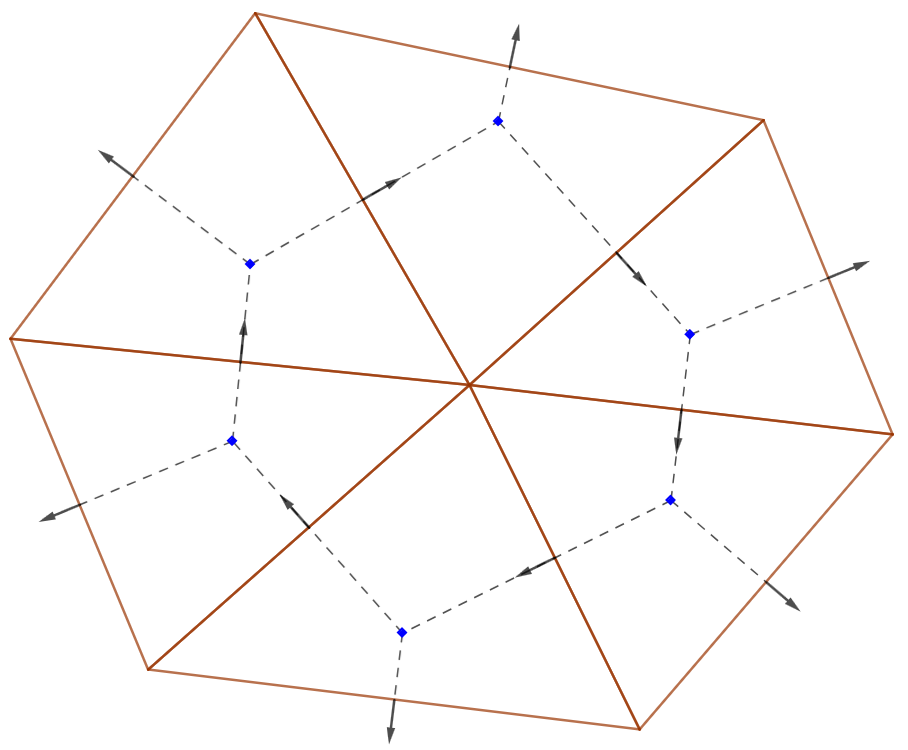
Figure 2: ICON-O’s horizontal discretization design. The scalar height field is located in the blue diamond shape, while the vector velocity field is decomposed in the midpoint edges of each triangle.

The ocean model equations contain the two-dimensional shallow water equations (SWE) used in this paper as a special case. The SWE are

(3a) $$\partial_{t}h=\nabla\cdot\mathbf{u}h$$

(3b) $$\partial_{t}\mathbf{u}=\nabla[g(h+b)+E_{k}]+(f+\omega)\mathbf{u}^{\perp},$$

where $h$ and $\mathbf{u}=(u,v)$ are scalar height and vector velocity field consisting of zonal ($u$) and meridional ($v$) velocity components, respectively. Here, $g$ is the Earth’s gravity acceleration, $b$ is the topography, $E_{k}=|\mathbf{u}|^{2}/2$ is the kinetic energy, $f$ is the Coriolis parameter, $\omega$ is the relative vorticity, and $\mathbf{u}^{\perp}=\mathbf{k}\times\mathbf{u}$ is the perpendicular velocity, where $\mathbf{k}$ is the unitary vertical vector.

The numerical scheme of ICON-O in its shallow-water configuration satisfies discrete conservation laws for mass, total energy, potential vorticity and potential enstrophy [15]. A study of its accuracy was provided by Lapolli et al. [24].

2.2 Network architecture

We define the ML model on a local domain as shown in Figure 3. In doing so, we assume that our choice of $\tau$ is sufficiently small so that the difference between the integrated high-resolution and low-resolution velocity field is local. The advantage of this approach is that the model otherwise tends to overfit to global structures. In addition, model prediction of local patches can be done in parallel, which is particularly useful when the model is running on high performance computing systems.

Figure 3: Our super-resolution network consists of a U-Net core model and two modules handling the transition between the ICON-O grid and the regular grid. Nearest neighbor interpolation is used to map the local patch $\mathbf{u}_{n,m}$ to a regular grid. The corrected patch is obtained by sampling data points from the output of the U-Net according to their coordinates.

We define a local patch by $\mathbf{u}_{n,m}$ with $n,m\in\{0,\dots,7\}$ as a subset of the unstructured grid of ICON-O. We use nearest neighbor interpolation to interpolate the subset to a high-resolution regular grid of $1024\times 1024\,$pixels. We use a $10\%$ overlap of the patches during training. The output data $\bar{\mathbf{u}}_{n,m}$ is sampled from the output of the core model based on their relative coordinates.

The core model has a U-net structure [25] with skip connections to take advantage of the computational efficiency of convolutions in image to image tasks. We define the convolutional layers of the U-net without biases. As a consequence, the trivial field correction is itself a trivial field $\Theta(\mathbf{0})=\mathbf{0}$.

The detailed structure of the U-net is shown in Figure 4.

Figure 4: U-Net core of the ML model. In the encoder and decoder branch, we use a kernel size of $7\times 7$ and $3\times 3$, respectively. The dotted arrows indicate concatenation of tensors.

The basic element of our U-Net consists of two consecutive residual blocks, or ResNet blocks [8], with a swish activation function [6] and a $1\times 1$ convolutional layer for the residual connection. We use average pooling layers with a kernel size of $4$ to effectively decrease the spatial dimension.

Upsampling, i.e., increasing the spatial dimension in the decoder part of the U-Net, is realized by sub-pixel convolutional blocks [27]. These consist of a convolutional layer, which increases the channel dimension by a factor of $r^{2}$, where $r$ is the factor by which the resolution is to be increased in both spatial dimensions. A consecutive pixel-shuffle operation rearranges the tensor with a shape of $(r^{2}N_{c},N_{x},N_{y})$ such that the channel dimension is decreased by a factor of $1/r^{2}$, whereas both spatial dimensions are increased by a factor of $r$. We use the kernel weight initialization proposed by Aitken [1] to ensure the absence of checkerboard artifacts.

The output of the encoder branch is concatenated with the respective upsampled output of the decoder layer and fed into the next layer. Note that for the input and output, we are using grouped convolutions to efficiently learn input and output features for both velocity components.

3 Experiment Design

We analyze the performance of our approach for the Galewsky testcase  [11]. This testcase describes the transition from a geostrophically balanced steady state to a barotropic instability. This transition is triggered by a small perturbation that is added to the balanced initial condition and that needs several days to build up. The instability of barotropic jets is a classical and well studied process in geophysical fluid dynamics that occurs in both the atmosphere and the ocean.

The initial condition is defined as follows

(4) $$u(\phi)=\begin{cases}0&\phi\leq\phi_{0}\\ u_{\max}/e_{n}\cdot\exp{\left(1/[(\phi-\phi_{0})(\phi-\phi_{1})]\right)}&\phi_{0}\leq\phi\leq\phi_{1}\\ 0&\phi\geq\phi_{1},\end{cases}$$

where $u_{\max}=80$ ms^-1, $e_{n}=\exp\left(-4/(\phi_{1}-\phi_{0})^{2}\right)$, $\phi_{0}=\pi/7-n_{\phi}\pi/36$, $n_{\phi}\in\{-1,0,1\}$, and $\phi_{1}=\pi/2-\phi_{0}$. This is balanced by the height field

(5) $$gh(\phi)=gh_{0}-\int^{\phi}au(\phi^{\prime})\left[f+\frac{\tan\phi^{\prime}}{a}u(\phi^{\prime})\right]d\phi^{\prime},$$

where $a=6.371\times 10^{6}$ m is the radius of the Earth and the resultant integral is a function of the latitude $\phi$. Here, the integral is unfeasible to calculate analytically, therefore, we chose to compute it using Rombergs’ quadrature, from the bounds of 90^∘S, where $u=0$ to $\phi$.

To trigger the instability and development of turbulence we add the perturbation

(6) $$h^{\prime}(\lambda,\phi)=\hat{h}\exp\left(-[(\lambda_{2}-\lambda)/\alpha]^{2}\right)\exp\left(-[(\phi_{2}-\phi)/\beta]^{2}\right)\cos\phi,$$

where $\lambda$ is the longitude, and $\lambda_{2}=n_{\lambda}\pi/4-\pi$, $n_{\lambda}\in\{0,\dots,7\}$, $\phi_{2}=\pi/4-n_{\phi}\pi/36$, $\alpha=1/3$, $\beta=1/15$, and $\hat{h}=$120\text{\,}\mathrm{m}$$.

3.1 Training of the ML model

We employ the training scheme shown in Figure 1 (blue box). Starting from the same initial conditions, we integrate the shallow water equations Eq. 3b on both, the high-resolution ($2.5\text{\,}\mathrm{km}$) and the low-resolution ($20\text{\,}\mathrm{km}$) grid. At $t=\tau=$12\text{\,}\mathrm{h}$$ we generate outputs from both grids $\mathbf{u}_{\text{hr}}(t+\tau)$ and $\mathbf{u}_{\text{lr}}(t+\tau)$. We obtain the ground truth $\mathbf{u}^{\prime}(t+\tau)$ by interpolating the $2.5\text{\,}\mathrm{km}$ output to the $20\text{\,}\mathrm{km}$ grid using distance weighted interpolation Climate Data Operators (CDO) [26]. After forward feeding the ML model with the low resolution output $\bar{\mathbf{u}}=\Theta(\mathbf{u}_{\text{lr}}(t+\tau))$, we calculate gradients based on the loss

(7) $$\mathcal{L}=\mathcal{L}_{\text{abs}}+\gamma\mathcal{L}_{\text{rel}}$$

where

(8) $$\mathcal{L}_{\text{abs}}=\frac{1}{N}\sum_{i}^{N}\left(|\bar{u}_{i}-u^{\prime}_{i}|\right)^{2}+\left(|\bar{v}_{i}-v^{\prime}_{i}|\right)^{2}$$

and

(9) $$\mathcal{L}_{\text{rel}}=\frac{1}{N}\sum_{i}^{N}\left(\min\left[1,\frac{|\bar{u}_{i}-u^{\prime}_{i}|}{u^{\prime}_{i}+\epsilon}\right]+\min\left[1,\frac{|\bar{u}_{i}-u^{\prime}_{i}|}{u^{\prime}_{i}+\epsilon}\right]\right).$$

Here, $u^{\prime}_{i},v^{\prime}_{i}$ and $\bar{u}_{i},\bar{v}_{i}$ denote the i-th element of the zonal and the meridional velocity components and $\epsilon=10^{-12}$ an offset to avoid division by zero. We chose a squared error loss in the computation of Eq. 8 as an absolute error measure to penalize large valued errors. To stabilize the training process, we restrict maximum errors to $1$. In addition, we add a non-squared relative error loss to Eq. 7, weighted by $\gamma=0.1$, to penalize deviations across all orders of magnitude.

The training data set of the ML model is provided by running variations of the original Galewsky by modifying the location of the jet Eq. 4 by setting

$$\phi_{0} = \pi/7-n_{\phi}\pi/36$$

$$\phi_{1} = \pi/2-\phi_{0}$$

with $n_{\phi}\in\{-1,0,1\}$, and the location of the perturbation Eq. 6 by setting

$$\lambda_{2} = n_{\lambda}\pi/4-\pi$$

$$\phi_{2} = \pi/4-n_{\phi}\pi/36.$$

We chose $n_{\phi}$ and $n_{\lambda}$ for generating the training and validation data according to Table 1. For validation, we use the original Galewsky test case. We run the simulations over $20\text{\,}\mathrm{days}$ with a timestep of $10\text{\,}\mathrm{s}$ and an output frequency of $12\text{\,}\mathrm{h}$.

	jet location	perturbation location	total number of snapshots
	$n_{\phi}$	$n_{\lambda}$
training	$\{-1,1\}$	$\{0,\dots,7\}$	$1184$
validation	0	0	37

Table 1: Simulation setups for generating the training and validation data. We use a $12\text{\,}\mathrm{h}$ output frequency and a maximum simulation time of $20\text{\,}\mathrm{d}\mathrm{a}\mathrm{y}\mathrm{s}$.

The total number of unique patches, which are randomly sampled, amounts to $N=$32\text{\,}\mathrm{(}\mathrm{p}\mathrm{a}\mathrm{t}\mathrm{c}\mathrm{h}\mathrm{e}\mathrm{s}\mathrm{)}$\cdot$1184\text{\,}\mathrm{(}\mathrm{s}\mathrm{n}\mathrm{a}\mathrm{p}\mathrm{s}\mathrm{h}\mathrm{o}\mathrm{t}\mathrm{s}\mathrm{)}$=37888$ and $2368$ for training and validation, respectively. We train the model for $50\,000\text{\,}$ mini-batch iterations with a batch size of $32$ on $4\times\text{A100}$ GPUs using a decaying learning rate with an initial learning rate of $10^{-4}$ (Figure 5).

3.2 ML correction during runtime

Given the trained ML model, we are now running ICON-O coupled with the ML model (Figure 1, top panel only). We again use the original Galewsky test case with $n_{\lambda}=n_{\phi}=0$, a model time step of $10\text{\,}\mathrm{s}$ and a correction frequency of $12\text{\,}\mathrm{h}$.

For evaluating the performance of the ML coupling with ICON, we compute the accuracy error norms for the simulated fields, i.e., velocity and height. We compute errors in both $L_{2}$-and $L_{\text{max}}$-norm, as they will provide information about the integrated error as well as local errors. These norms are defined as:

(10a) $$L_{2}=\sqrt{\frac{S[(f^{[n]}-f^{[r]})^{2}]}{S[(f^{[r]})^{2}]}},$$

(10b) $$L_{\max}=\frac{\max_{j}\left|f^{[n]}_{j}-f^{[r]}_{j}\right|}{\max_{j}\left|f^{[r]}_{j}\right|},$$

where $f^{[n]}_{j}$ and $f^{[r]}_{j}$ is the reference (high resolution) and coarse fields at cell $j$, respectively. $S$ is defined as

$$S[f]=\frac{\sum_{j}A_{j}f_{j}}{\sum_{j}A_{j}};$$

where $A_{j}$ is the area of the $j$-th cell. The simulated field is the low resolution (LR $20\text{\,}\mathrm{km}$) simulated outputs, while the reference solution is the interpolated high resolution (HR $2.5\text{\,}\mathrm{km}$) to LR simulated outputs. For a proper comparison, we interpolate the HR outputs with a distance weighted interpolation from the Climate Data Operator (CDO) software.

Additionally, to evaluate the conservation properties of our schemes, we track energy over time. The globally integrated kinetic and potential energy are

$$\overline{E_{k}} =\sum_{j}\frac{|\mathbf{u}_{j}|^{2}}{2}A_{j},$$

$$\overline{E_{p}} =g\sum_{j}h_{j}A_{j}.$$

The transfer of energy from small to large scale and the transfer from enstrophy from large to small scales follow well known scaling laws (see e.g. [30])We evaluate the effect that the ML correction has on the representation of these spectra. In order to calculate energy and enstrophy we use the formulation by Jacob et al. [10, 31].

4 Numerical results

We first analyze the performance of the ML model correcting the low resolution Galewsky test case that periodically has been initialized by a high resolution run as shown in Figure 1. This serves as a best case for the ML correction performance, as the re-initialization from high resolution avoids error propagation. We then compare these results to the coupled run, where the output of the ML is used for initialization Figure 1 (top panel only).

4.1 ML Training

The training progress is shown in Figure 5. The presence of large fluctuations in the training loss is because of the random sampling of local patches. Even though we restrict maximum losses to values of 1, low amplitudes of $v$ result in a high contribution to the relative error Eq. 9. To avoid overfitting of the data, we stopped the optimization after $50\,000\text{\,}$ mini-batch iterations.

Figure 6 and 7 show the global snapshots of the uncorrected ML input and the ML output of the $v$-component of the velocity field $\mathbf{u}$ at $t=$12\text{\,}\mathrm{h}$$ and $t=$7\text{\,}\mathrm{days}$$. The ML model is able to remove the numerical oscillations induced by the coarse resolution at both time points, with $v$ ranging over several orders of magnitude. The presence of patches in the ML output indicates that the ML model is robust to local variations of the input data.

Figure 5: ML model learning progress as a function of mini-batch iteration. Validation was done at a frequency of $200\text{\,}$iterations, averaged over $10\text{\,}\mathrm{i}$terations. To compare both losses, we applied a moving average window to the training loss. The learning rate as a function of the training iteration is shown in the bottom graph.

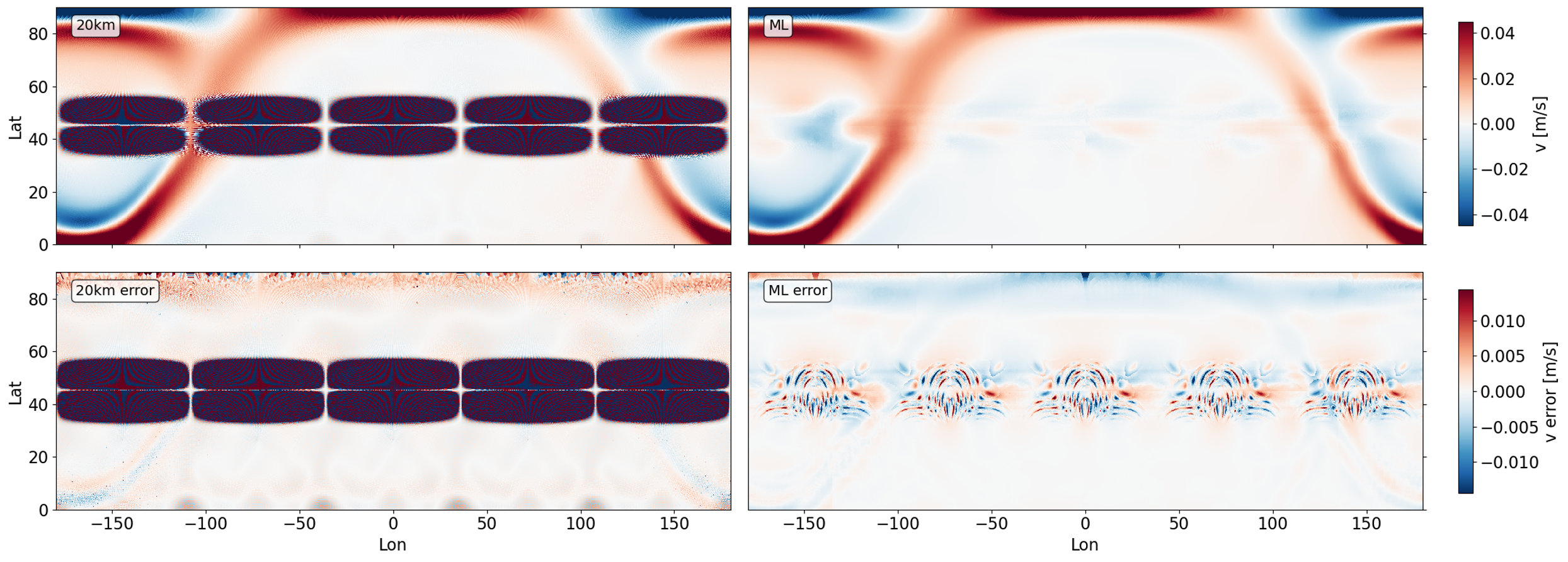
Figure 6: $v$-component of the velocity field at $t=12$h (top row) and corresponding error maps (bottom row) of the $20\text{\,}\mathrm{km}$ simulation (left) and the ML output (right). The integration of the same initial condition ($t=0$) on a $2.5\text{\,}\mathrm{km}$ grid serves as ground truth. Refer to Figure 1 for further details of the training scheme.

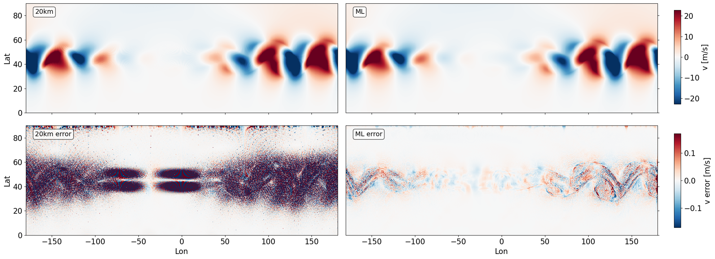
Figure 7: $v$-component of the velocity field at $t=7$d (top row) and corresponding error maps (bottom row) of the $20\text{\,}\mathrm{km}$ simulation (left) and the ML output (right). The integration of the same initial condition ($t=$6.5\text{\,}\mathrm{days}$$) on a $2.5\text{\,}\mathrm{km}$ grid serves as ground truth. Refer to Figure 1 for further details of the training scheme.

4.2 Numerical Accuracy

The uncoupled ICON simulation shows a low of error in both norms for all fields, quickly increasing from day 4 to day 8, where it then saturates until the end of the computational simulation, see Figure 8. For both $L_{2}$ and $L_{\max}$ norms, the errors of the uncoupled simulations for the last day of integration are found in Table 2. Note that, since the meridional component of the velocity is zero at the initial state, the $v$-component is not normalized as the other fields. Regardless, we observe a near first order accuracy of these fields on both norms, which is expected from the model. Additionally, it can be observed that the order of accuracy is slightly lower for the maximum norm. It may be the case that the testcase we are evaluating is prone to many numerical oscillations, or that the reference simulation of $2.5\text{\,}\mathrm{km}$ is not fine enough to achieve a first order accuracy in the maximum norm. Another possibility is that the choice of interpolation used for the $2.5\text{\,}\mathrm{km}$ might not be optimal.

	$L_{2}$			$L_{\max}$
	$10\text{\,}\mathrm{km}$	ML${}_{\text{coupled}}$	$20\text{\,}\mathrm{km}$	$10\text{\,}\mathrm{km}$	ML${}_{\text{coupled}}$	$20\text{\,}\mathrm{km}$
$u$	4.40$\times$10-1	4.43$\times$10-1	7.20$\times$10-1	0.78	0.76	1.25
$v$	7.47	7.58	13.99	58.79	73.19	76.59
$h$	0.84$\times$10-2	1.01$\times$10-2	0.81$\times$10-2	7.10$\times$10-2	6.78$\times$10-2	9.23$\times$10-2

Table 2: Errors of the uncoupled simulation between 2.5km and 10km/20km resolutions for the different fields at the last day of integration.

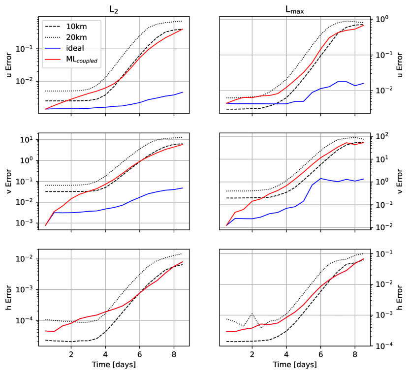
Figure 8: Accuracy error for the ICON-O simulations with $10\text{\,}\mathrm{km}$ and $20\text{\,}\mathrm{km}$ resolution, the ICON-O simulation with ML replacement every $12\text{\,}\mathrm{h}$ (ML_coupled). The ideal curve shows the error of the ML model on the validation set, which results from correcting the $12\text{\,}\mathrm{h}$ output of the $20\text{\,}\mathrm{km}$ that is periodically initialized by the high-resolution $2.5\text{\,}\mathrm{km}$ ground truth. See Section 3.1 for further details. Note that the blue curve is missing in the sea surface height error h, since the ML model corrects only the velocity components.

In contrast, the coupled ICON/ML run has its first correction, displaying a significant improved error in comparison to the uncoupled $20\text{\,}\mathrm{km}$. The error of the velocity components, although displaying substantially lower values than the uncoupled $10\text{\,}\mathrm{km}$, quickly increase as the field is integrated in time. This increase is also reflected in the height field, showing an increase in the error slightly larger than the uncoupled $20\text{\,}\mathrm{km}$ simulation. Despite this, this increase in error is not sustained, as the model is integrated in time, the overall fields accuracy tend to the order of the uncoupled $10\text{\,}\mathrm{km}$ simulation. It is also observed that for some days in the later stages of the simulation, the accuracy of the coupled run overtakes even the uncoupled $10\text{\,}\mathrm{km}$, especially in the $L_{2}$ norm of the $u$ and $v$ velocity components. Additionally, despite the height field not being directly affected by the ML, it is impacted by the corrections performed in the velocity field. As in the first days of integration, the accuracy of the height field decreases, but eventually improves and also reaches the order of accuracy of the uncoupled finer simulation. This indicates a conflicting behavior of the two fields: As the height field is untouched by the ML, it pushes the solution towards a less accurate state, while the velocity components push the solution into a more accurate solution. Although this may indicate a reduction of the accuracy of the simulation, the overall improvement is clear and the coupled ML simulation is shown capable of refining error metrics.

The improvement in the domain becomes particularly evident when examining the vorticity field in the 7th day of simulation. Here, we observe the early stages of the triggering of the fluid instability. We see the vorticity field generating vortexes as a consequence of the instability, with these vortexes being transported eastward (see Figure 9). These vortical formations generate tight gradients which, besides ICON’s own numerical noise, are also a source of spurious oscillations [11]. For coarser simulations, these oscillations are greater and the instability is shown to be more developed away from the initial region of perturbation, visible in the uncoupled $20\text{\,}\mathrm{km}$ simulation.

This illustrates the effects of the grid resolution in the fluid simulation. From this perspective, it is noticeable that the coupled model has shown to accurately portray the onset of instability and delaying local instabilities generated by the interaction between the spurious oscillations of both the unstructured nature of the grid and tight gradients by the testcase. However, the ML corrections add its own set of artifacts, see Figure 10, which is likely playing a role in the accuracy of the model. Therefore, we may interpret that the difficulty to maintain low error in the first few days is a consequence of these artifacts, especially in the early stages of the simulation. In the first correction, the ML model is capable of substantially reducing the noise created by the ICON model. Due to the lack of diffusivity in the model, however, these noises do not disappear, and they are still present in the solution. Although, these oscillations are apparent they do not amplify nor seem to meaningfully disrupt the solution of the integrated fields, since we can achieve a $10\text{\,}\mathrm{km}$-order-error simulation.

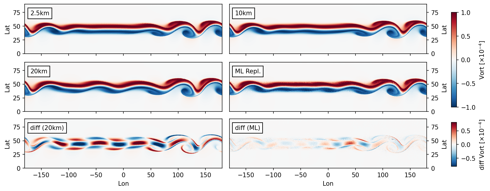
Figure 9: Vorticity map at day 7 of integration for the uncoupled $2.5\text{\,}\mathrm{km}$, $10\text{\,}\mathrm{km}$, $20\text{\,}\mathrm{km}$ simulations and the coupled $20\text{\,}\mathrm{km}$ simulation, and the vorticity difference between the uncoupled $20\text{\,}\mathrm{km}$ and $2.5\text{\,}\mathrm{km}$ simulations, and the coupled $20\text{\,}\mathrm{km}$ and uncoupled $2.5\text{\,}\mathrm{km}$ simulations.

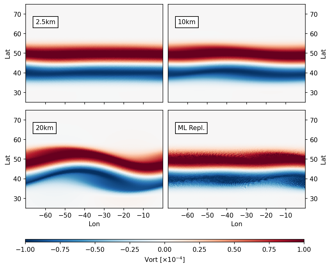
Figure 10: Vorticity as in Figure 9; zoomed at the region 100^∘E-170^∘E and 25^∘N-75^∘N.

Despite the improvement, it is important to understand if this artificial impact of the coupled model, especially concerning its numerical oscillations, may disrupt the natural flow of energy in different scales. In Figure 11 (upper panel) we observe the energy spectrum in day 6 of the model simulation. From the theory, it is expected a direct cascade of energy with a slope of $k^{-3}$. In our analysis, all models represent the same energy slope up to the index 200 ($\approx$ 200 km resolution). In this scale, the coupled ML run starts to deviate, while the uncoupled $20\text{\,}\mathrm{km}$ simulation still maintains its slope, deviating only at index 500 ($\approx$ 80 km resolution). This reinforces the argument that the machine learning is predominantly acting in the smaller scales. Despite this, the method still consistently preserves the energy flow in the large scales.

Similarly, the enstrophy spectrum, see Figure 11, (lower panel), displays a similar enstrophy cascade up to the 200 km resolution. Around these scales, the uncoupled $20\text{\,}\mathrm{km}$ simulation is the first to deviate from the theory, followed by the coupled $20\text{\,}\mathrm{km}$ simulation. In these scales, the uncoupled model loses substantially its enstrophy in higher wavenumbers, while the coupled simulation display an increase for higher resolutions. This indicates that the ML is adding energy into the smaller scales, likely in the form of the previously observed spurious oscillations. Due to the non-dissipative nature of our system, the high wavenumber regime is not dissipated into mixing and, therefore, remains in the domain. Although in a more complex model, waves of this order may contribute to the mixing of water, and aid in the turbulence of the system, these can be solved by an appropriate choice of low pass filter, such as a higher order dissipative operator to dim these higher wavenumber waves.

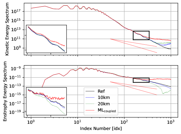
Figure 11: Kinetic energy (top panel) and enstrophy (bottom panel) spectrum of the uncoupled $20\text{\,}\mathrm{km}$ and $10\text{\,}\mathrm{km}$ runs, and the ML coupling simulation. The dashed red lines are the k^-3 and k^-5/3 slopes.

In order to verify if this increased energy in higher wavenumbers has an overall effect in the energy conservation of our scheme, we evaluate the total energy time evolution (Figure 12). In the coupled run, it is observed that the kinetic energy of the system increases up to around day 6 and decreases in the subsequent days. Conversely, both uncoupled simulations show a relatively stable integrated kinetic energy up to day 5, with a slight uptick preceding the instability, followed by a consistent decline in energy, thereafter. The integrated energy variation of the uncoupled run is about as half of the coupled runs, indicating that the ML is inputting energy in the domain. As observed in the energy spectrum, this input of energy is in the form of low resolution (high wavenumbers) waves, likely generated by the spurious oscillations of the ML correction. Despite this, the observed increase in energy is not monotonic, so we see, at least for the integrated period, no threat in destabilizing the solution.

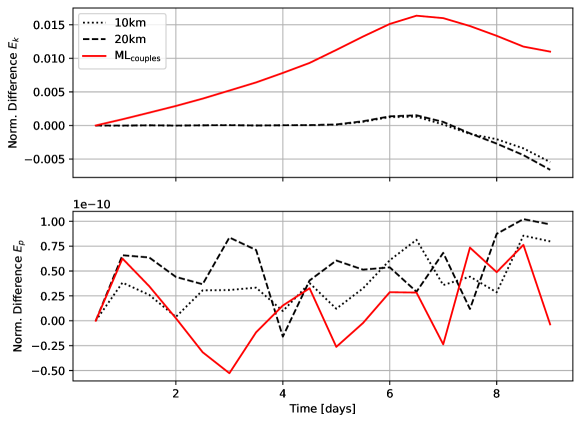
Figure 12: Normalized difference for both globally integrated kinetic (upper panel) and potential energy (lower panel).

5 Conclusions

We present a hybrid modeling approach, combining a mesh based model with an ML correction, that allows us to run a global numerical simulation of the shallow water equations on a twice coarser mesh without loss of accuracy. The continuity between adjacent predictions in the global output confirms the reliability of employing a local ML model approach to correct a global velocity field. As our ML model operates solely through convolutions, adapting it for large-scale fields is straightforward by adjusting the patch size to fit to available computational resources. Employing independent patches enables parallelization of ML predictions for efficient corrections.

The trained ML model effectively reduces the discretization errors of the integration of the shallow water equations by orders of magnitude.

Additionally, using relative errors in optimizing the parameters of the model ensures a consistent model performance across different scales, which is crucial to preserve the stability of the jet of the Galewsky test case.

However, the error increases when the output of the ML model is integrated in time in the coupled run. The remaining artifacts produced by the ML model still affect the solution and likely lowers the accuracy of the coupling. Additionally, the ML model acts as a source of kinetic energy. Although it does not push the solution to numerical instability, this could become an issue for more complex regimes. Lastly, despite the direct cascade of both energy enstrophy being respected for large scales, they are affected in the high wavenumbers, likely due to the noise produced by the ML, which also could potentially destabilize the solution in longer simulations.

In the future, we need to address the numerical and physical implications of the ML model’s output. Integrating physical constraints into the ML model will help to conserve the physical properties of our hybrid approach. In addition, training objectives penalizing artifacts and forcing convergence of the ML correction will help to enhance the stability integrating the ML output in time. Additionally, incorporating statistical ML approaches to estimate model uncertainty may offer further insights into stabilizing the ML correction process.

The results presented in this work show great potential to improve climate modelling performance by using ML to account for discretization errors.

In the near future, we will explore the limitations of this method in terms of accuracy, scalability and physical validity in a realistic global 3D simulation.

References

- [1] A. Aitken, C. Ledig, L. Theis, J. Caballero, Z. Wang, and W. Shi, Checkerboard artifact free sub-pixel convolution: A note on sub-pixel convolution, resize convolution and convolution resize, 2017, https://arxiv.org/abs/1707.02937.
- [2] C. S. Bretherton, B. Henn, A. Kwa, N. D. Brenowitz, O. Watt-Meyer, J. McGibbon, W. A. Perkins, S. K. Clark, and L. Harris, Correcting coarse-grid weather and climate models by machine learning from global storm-resolving simulations, Journal of Advances in Modeling Earth Systems, 14 (2022), p. e2021MS002794, https://doi.org/10.1029/2021MS002794.
- [3] S. K. Clark, N. D. Brenowitz, B. Henn, A. Kwa, J. McGibbon, W. A. Perkins, O. Watt-Meyer, C. S. Bretherton, and L. M. Harris, Correcting a 200 km resolution climate model in multiple climates by machine learning from 25 km resolution simulations, Journal of Advances in Modeling Earth Systems, 14 (2022), p. e2022MS003219, https://doi.org/10.1029/2022MS003219.
- [4] J. J. Danker Khoo, K. H. Lim, and J. T. Sien Phang, A review on deep learning super resolution techniques, in 2020 IEEE 8th Conference on Systems, Process and Control (ICSPC), 2020, pp. 134–139, https://doi.org/10.1109/ICSPC50992.2020.9305806.
- [5] C. Dong, C. C. Loy, K. He, and X. Tang, Learning a deep convolutional network for image super-resolution, in Computer Vision – ECCV 2014, D. Fleet, T. Pajdla, B. Schiele, and T. Tuytelaars, eds., Cham, 2014, Springer International Publishing, pp. 184–199.
- [6] S. Elfwing, E. Uchibe, and K. Doya, Sigmoid-weighted linear units for neural network function approximation in reinforcement learning, Neural Networks, 107 (2018), pp. 3–11, https://doi.org/10.1016/j.neunet.2017.12.012. Special issue on deep reinforcement learning.
- [7] S. Gao, X. Liu, B. Zeng, S. Xu, Y. Li, X. Luo, J. Liu, X. Zhen, and B. Zhang, Implicit diffusion models for continuous super-resolution, in 2023 IEEE/CVF Conference on Computer Vision and Pattern Recognition (CVPR), 2023, pp. 10021–10030, https://doi.org/10.1109/CVPR52729.2023.00966.
- [8] K. He, X. Zhang, S. Ren, and J. Sun, Deep residual learning for image recognition, 2015, https://arxiv.org/abs/1512.03385.
- [9] C. Hohenegger, P. Korn, L. Linardakis, R. Redler, R. Schnur, P. Adamidis, J. Bao, S. Bastin, M. Behravesh, M. Bergemann, J. Biercamp, H. Bockelmann, R. Brokopf, N. Brüggemann, L. Casaroli, F. Chegini, G. Datseris, M. Esch, G. George, M. Giorgetta, O. Gutjahr, H. Haak, M. Hanke, T. Ilyina, T. Jahns, J. Jungclaus, M. Kern, D. Klocke, L. Kluft, T. Kölling, L. Kornblueh, S. Kosukhin, C. Kroll, J. Lee, T. Mauritsen, C. Mehlmann, T. Mieslinger, A. K. Naumann, L. Paccini, A. Peinado, D. S. Praturi, D. Putrasahan, S. Rast, T. Riddick, N. Roeber, H. Schmidt, U. Schulzweida, F. Schütte, H. Segura, R. Shevchenko, V. Singh, M. Specht, C. C. Stephan, J.-S. von Storch, R. Vogel, C. Wengel, M. Winkler, F. Ziemen, J. Marotzke, and B. Stevens, ICON-Sapphire: simulating the components of the Earth system and their interactions at kilometer and subkilometer scales, Geoscientific Model Development, 16 (2023), pp. 779–811, https://doi.org/10.5194/gmd-16-779-2023.
- [10] R. Jakob-Chien, J. J. Hack, and D. L. Williamson, Spectral transform solutions to the shallow water test set, Journal of Computational Physics, 119 (1995), pp. 164–187, https://doi.org/10.1006/jcph.1995.1125.
- [11] R. K. S. Joseph Galewsky and L. M. Polvani, An initial-value problem for testing numerical models of the global shallow-water equations, Tellus A: Dynamic Meteorology and Oceanography, 56 (2004), pp. 429–440, https://doi.org/10.3402/tellusa.v56i5.14436.
- [12] C. Kadow, D. M. Hall, and U. Ulbrich, Artificial intelligence reconstructs missing climate information, Nat. Geosci., (2020), https://doi.org/10.1038/s41561-020-0582-5.
- [13] K. Kashinath, M. Mustafa, A. Albert, J.-L. Wu, C. Jiang, S. Esmaeilzadeh, K. Azizzadenesheli, R. Wang, A. Chattopadhyay, A. Singh, A. Manepalli, D. Chirila, R. Yu, R. Walters, B. White, H. Xiao, H. A. Tchelepi, P. Marcus, A. Anandkumar, P. Hassanzadeh, and n. Prabhat, Physics-informed machine learning: case studies for weather and climate modelling, Philosophical Transactions of the Royal Society A: Mathematical, Physical and Engineering Sciences, 379 (2021), p. 20200093, https://doi.org/10.1098/rsta.2020.0093.
- [14] P. Korn, N. Brüggemann, J. H. Jungclaus, S. J. Lorenz, O. Gutjahr, H. Haak, L. Linardakis, C. Mehlmann, U. Mikolajewicz, D. Notz, D. A. Putrasahan, V. Singh, J.-S. von Storch, X. Zhu, and J. Marotzke, ICON-O: The Ocean Component of the ICON Earth System Model—Global Simulation Characteristics and Local Telescoping Capability, Journal of Advances in Modeling Earth Systems, 14 (2022), https://doi.org/10.1029/2021MS002952.
- [15] P. Korn and L. Linardakis, A conservative discretization of the shallow-water equations on triangular grids, Journal of Computational Physics, 375 (2018), pp. 871–900, https://doi.org/10.1016/j.jcp.2018.09.002.
- [16] R. Lam, A. Sanchez-Gonzalez, M. Willson, P. Wirnsberger, M. Fortunato, F. Alet, S. Ravuri, T. Ewalds, Z. Eaton-Rosen, W. Hu, A. Merose, S. Hoyer, G. Holland, O. Vinyals, J. Stott, A. Pritzel, S. Mohamed, and P. Battaglia, Graphcast: Learning skillful medium-range global weather forecasting, 2023, https://arxiv.org/abs/2212.12794.
- [17] C. Ledig, L. Theis, F. Huszar, J. Caballero, A. Cunningham, A. Acosta, A. Aitken, A. Tejani, J. Totz, Z. Wang, and W. Shi, Photo-realistic single image super-resolution using a generative adversarial network, in 2017 IEEE Conference on Computer Vision and Pattern Recognition (CVPR), Los Alamitos, CA, USA, jul 2017, IEEE Computer Society, pp. 105–114, https://doi.org/10.1109/CVPR.2017.19.
- [18] N. Margenberg, R. Jendersie, C. Lessig, and T. Richter, DNN-MG: A hybrid neural network/finite element method with applications to 3d simulations of the Navier–Stokes equations, Computer Methods in Applied Mechanics and Engineering, 420 (2024), p. 116692, https://doi.org/https://doi.org/10.1016/j.cma.2023.116692.
- [19] S. Moghim and R. L. Bras, Bias correction of climate modeled temperature and precipitation using artificial neural networks, Journal of Hydrometeorology, 18 (2017), pp. 1867 – 1884, https://doi.org/10.1175/JHM-D-16-0247.1.
- [20] P. Neumann, P. Düben, P. Adamidis, P. Bauer, M. Brück, L. Kornblueh, D. Klocke, B. Stevens, N. Wedi, and J. Biercamp, Assessing the scales in numerical weather and climate predictions: will exascale be the rescue?, Philosophical Transactions of the Royal Society A: Mathematical, Physical and Engineering Sciences, 377 (2019), p. 20180148, https://doi.org/10.1098/rsta.2018.0148.
- [21] J. Pathak, M. Mustafa, K. Kashinath, E. Motheau, T. Kurth, and M. Day, Using machine learning to augment coarse-grid computational fluid dynamics simulations, 2020, https://arxiv.org/abs/2010.00072.
- [22] J. Pathak, S. Subramanian, P. Harrington, S. Raja, A. Chattopadhyay, M. Mardani, T. Kurth, D. Hall, Z. Li, K. Azizzadenesheli, P. Hassanzadeh, K. Kashinath, and A. Anandkumar, Fourcastnet: A global data-driven high-resolution weather model using adaptive fourier neural operators, 2022, https://arxiv.org/abs/2202.11214.
- [23] D. A. Randall, C. M. Bitz, G. Danabasoglu, A. S. Denning, P. R. Gent, A. Gettelman, S. M. Griffies, P. Lynch, H. Morrison, R. Pincus, and J. Thuburn, 100 years of earth system model development, Meteorological Monographs, 59 (2018), pp. 12.1 – 12.66, https://doi.org/10.1175/AMSMONOGRAPHS-D-18-0018.1.
- [24] F. Rodrigues Lapolli, P. da Silva Peixoto, and P. Korn, Accuracy and stability analysis of horizontal discretizations used in unstructured grid ocean models, Ocean Modelling, 189 (2024), p. 102335, https://doi.org/10.1016/j.ocemod.2024.102335.
- [25] O. Ronneberger, P. Fischer, and T. Brox, U-net: Convolutional networks for biomedical image segmentation, 2015, https://arxiv.org/abs/1505.04597.
- [26] U. Schulzweida, L. Kornblueh, and R. Quast, CDO user guide, 2019.
- [27] W. Shi, J. Caballero, F. Huszar, J. Totz, A. P. Aitken, R. Bishop, D. Rueckert, and Z. Wang, Real-time single image and video super-resolution using an efficient sub-pixel convolutional neural network, in 2016 IEEE Conference on Computer Vision and Pattern Recognition (CVPR), Los Alamitos, CA, USA, jun 2016, IEEE Computer Society, pp. 1874–1883, https://doi.org/10.1109/CVPR.2016.207.
- [28] A. Staniforth and J. Thuburn, Horizontal grids for global weather and climate prediction models: a review, Q.J.R. Meteorol. Soc., 138 (2012), pp. 1–26, https://doi.org/10.1002/qj.958.
- [29] Y. Tao, X. Gao, K. Hsu, S. Sorooshian, and A. Ihler, A deep neural network modeling framework to reduce bias in satellite precipitation products, Journal of Hydrometeorology, 17 (2016), pp. 931 – 945, https://doi.org/10.1175/JHM-D-15-0075.1.
- [30] G. K. Vallis, Atmospheric and oceanic fluid dynamics, Cambridge University Press, 2017.
- [31] L. Wang, Y. Zhang, J. Li, Z. Liu, and Y. Zhou, Understanding the performance of an unstructured-mesh global shallow water model on kinetic energy spectra and nonlinear vorticity dynamics, J Meteorol Res, 33 (2019), pp. 1075–1097, https://doi.org/10.1007/s13351-019-9004-2.
- [32] Z. Wang, J. Chen, and S. C. H. Hoi, Deep learning for image super-resolution: A survey, IEEE Transactions on Pattern Analysis and Machine Intelligence, 43 (2021), pp. 3365–3387, https://doi.org/10.1109/TPAMI.2020.2982166.
- [33] Y. Xu, Y. Wang, S. Hu, and Y. Du, Deep convolutional neural networks for bias field correction of brain magnetic resonance images, J. Supercomput., 78 (2022), p. 17943–17968, https://doi.org/10.1007/s11227-022-04575-4.
- [34] J. Yuval and P. A. O’Gorman, Stable machine-learning parameterization of subgrid processes for climate modeling at a range of resolutions, Nat Commun, 11 (2020), p. 3295, https://doi.org/10.1038/s41467-020-17142-3.
- [35] C. Zhang, P. Perezhogin, C. Gultekin, A. Adcroft, C. Fernandez-Granda, and L. Zanna, Implementation and evaluation of a machine learned mesoscale eddy parameterization into a numerical ocean circulation model, Journal of Advances in Modeling Earth Systems, 15 (2023), p. e2023MS003697, https://doi.org/10.1029/2023MS003697.