Raster Forge: Interactive Raster Manipulation Library and GUI for Python

Afonso Oliveira¹(a22308561@alunos.ulht.pt), Nuno Fachada^1,2, João P. Matos-Carvalho^1,2

¹COPELABS, Lusófona University, Campo Grande 376, Lisbon, 1749-024, Lisbon, Portugal
²Center of Technology and Systems (UNINOVA-CTS) and Associated Lab of Intelligent Systems (LASI), 2829-516 Caparica, Portugal

Abstract

Raster Forge is a Python library and graphical user interface for raster data manipulation and analysis. The tool is focused on remote sensing applications, particularly in wildfire management. It allows users to import, visualize, and process raster layers for tasks such as image compositing or topographical analysis. For wildfire management, it generates fuel maps using predefined models. Its impact extends from disaster management to hydrological modeling, agriculture, and environmental monitoring. Raster Forge can be a valuable asset for geoscientists and researchers who rely on raster data analysis, enhancing geospatial data processing and visualization across various disciplines.

Keywords
python, graphical user interface, remote sensing, geosciences, wildfire, raster

Code Metadata

Current code version	v0.6.1
Permanent link to code/repository used for this code version	https://github.com/afe-oliveira/raster-forge
Legal Code License	MIT License
Code versioning system used	Git
Software code languages, tools, and services used	Python
Compilation requirements, operating environments & dependencies	Python 3.8+, PySide6, NumPy, Rasterio, Spyndex, OpenCV Python, Matplotlib
Developer documentation/manual	https://afe-oliveira.github.io/raster-forge/
Support email for questions	a22308561@alunos.ulht.pt

   1.     Motivation and Significance

Raster grids are one of the most common data structures for image representation [1, 2]. Constructed as a matrix of cells or pixels, they are also often associated with the storage, processing and representation of spatial data. Their importance lies in their ability to allow direct matrix computations, thus enabling several important processing techniques, such as segmentation and classification [3, 4, 5], resampling [6] and interpolation [7]. Multispectral images are particularly suited for representation within raster grids, as each cell can store intensity values across different wavelengths. Moreover, this structure is also very significant for its ability to provide an approximate representation of spatial phenomena, especially when coupled with appropriate geographic information [8].

Python is an extremely versatile language with thousands upon thousands of software for a wide variety of applications. Among these are some very influential tools that allow the manipulation of raster data, from powerful libraries such as OSGeo GDAL [9], Rasterio [10] and OpenCV [11], to fully fledged Geographic Informaiton Systems (GISs) like the GRASS GIS [12], ArcGIS [13] and QGIS [14].

While these tools are undoubtedly powerful and feature-rich, they can present certain barriers to entry. For instance, some may find them difficult to install or use, especially those new to GIS or lacking technical expertise. Even seemingly straightforward libraries like Rasterio or OpenCV can present hurdles, as their functionalities often require some degree of research before successful implementation. In addition, the costs of licensing proprietary software such as ArcGIS can be prohibitive for individuals or organizations with limited budgets.

Figure 1: Major libraries used to build Raster Forge. Adapted from [15, 16, 17, 18, 19].

In this paper we present Raster Forge, an easy to use library and Graphical User Interface (GUI), which aims to fill this gap for a beginner-friendly raster manipulation tool for spatial analysis. The library is powerful, direct and thoroughly documented, making its usage very straightforward. Additionally, its intuitive GIS eliminates the need for extensive research beforehand, allowing users to employ it quickly and effortlessly.

Raster Forge places great emphasis on the geospatial capabilities inherent in the raster structure. Although primarily designed to aid in wildfire management, care has been taken to ensure its versatility for more general applications.

   2.     Software Description

Raster Forge is divided into two parts: the library and the GUI. The library of implemented functions is detailed in Subsection 2.1, while the GUI application is presented in Subsection 2.2.

   2.1     Library

The library component is comprised of two container classes, Layer and Raster, which are used to represent a single grid of information and a collection of such grids, respectively. These classes are described with additional detail in Subsection 2.1.1. The processing functions are primarily designed to work with Layer objects, but they also support NumPy arrays (NDArray) [20] as inputs and outputs.

The library’s raster manipulation capabilities are divided into six categories, as outlined in Table 1. These categories include the generation of image composites (Subsection 2.1.2), multispectral indices (Subsection 2.1.3), topographical features (Subsection 2.1.4), distance fields (Subsection 2.1.5), height maps (Subsection 2.1.6), and fuel maps (Subsection 2.1.7).

Table 1: Library raster manipulation processes. NDArray is an array type provided by NumPy [20] and represents a multidimensional, homogeneous array of fixed-size items.

Task	Inputs
	Name	Data Type
Composites	Layers	List[NDArray, Layer]
	Alpha	NDArray, Layer
	Gamma	List[float], Tuple[float]
	As Array	bool
Indicesa	Index ID	String
	Index Parameters	Dictionary
	Alpha	NDArray, Layer
	Thresholds	List[float], Tuple[float]
	Binarize	bool
	As Array	bool
Slope	DEM	NDArray, Layer
	Units	degrees, radians
	Alpha	NDArray, Layer
	As Array	bool
Aspect	DEM	NDArray, Layer
	Units	degrees, radians
	Alpha	NDArray, Layer
	As Array	bool
Distance Field	Layer	NDArray, Layer
	Alpha	NDArray, Layer
	Thresholds	List[float], Tuple[float]
	Invert	bool
	Mask Size	3, 5
	As Array	bool
Height	DTM	NDArray, Layer
	DSM	NDArray, Layer
	Distance	NDArray, Layer
	Alpha	NDArray, Layer
	As Array	bool
Fuel Map	Vegetation Coverage	NDArray, Layer
	Canopy Height	NDArray, Layer
	Distance	NDArray, Layer
	Water Features Mask	NDArray, Layer
	Artificial Structures Mask	NDArray, Layer
	Fuel Models	List[int], Tuple[int]
	Tree Height	float
	Alpha	NDArray, Layer
	As Array	bool
a The multispectral indices architecture is built around the Spyndex Python library [21].

2.1.1 Containers

The Layer class holds the data and metadata of a single raster map, including geographic information and direct statistics, as shown in Table 2. The architecture of this object ensures that all relevant information is easily accessible through its properties. A data import function has also been developed to facilitate the extraction of a single band as a Layer from a raster file (see Table 3).

Table 2: Layer object properties.

Name	Data Type
Array	NDArray
Bounds	Dictionary
CRS	String
Driver	String
No Data	int, float
Transform	(float, float, float, float, float, float)
Units	String
Resolution	int
Width	int
Height	int
Count	int
Mean	float
Median	float
Min	int, float
Max	int, float
Standard Deviation	float

Table 3: Layer object methods.

Task	Inputs		Description
	Name	Data Type
Import Layer	File Path	String	Imports one band from a specified file as a layer. Applies scale to dataset if specified.
	Band ID	int
	Scale	int

The Raster class acts as a container for a group of Layers and is associated with an uniform pixel size—or scale—that applies to all constituent layers for uniformity. The properties of this class are described in Table 4, and its main responsibilities include the bulk import of raster data and the manipulation of the Layer collection, as highlighted in Table 5.

Table 4: Raster object properties.

Name	Data Type
Layers	Dictionary[String: Layer]
Scale	int

Table 5: Raster object methods.

Task	Inputs		Description
	Name	Data Type
Import Layers	File Path	String	Imports a series of bands as defined on the Config dictionary.
	Config	Dictionary
Add Layer	Name	String	Adds a Layer to the Layers Dictionary.
	Layer	Layer, NDArray
Remove Layer	Name	String	Remove a Layer from the Layers Dictionary.
Edit Layer	Old Name	String	Changes the name identifier of a given Layer in the Layers dictionary.
	New Name	String

2.1.2 Composites

This feature allows the creation of true and false colour composites. It includes gamma correction functionality, allowing the user to select the gamma value to be applied to each individual layer through a power law transformation, $I_{\text{out}}=I_{\text{in}}^{\gamma}$, where $I_{\text{out}}$ represents the output intensity or colour value, $I_{\text{in}}$ represents the input intensity or colour value, and $\gamma$ represents the gamma value applied for adjustment.

2.1.3 Multispectral Indices

Users can choose from a broad range of indices provided by the Spyndex [21] package and compute them directly using defined Layers. It also allows the application of a threshold to the index output, which facilitates the generation of binary masks.

2.1.4 Topographical Features

A user is able compute both the slope and the aspect (orientation of slopes) of a region defined by Digital Elevation Model (DEM) data. This implementation utilizes the direct slope calculation formula given by equation 1 and the aspect calculation given by equation 2. In these equations, the variable array represents a set of values, usually a DEM or a grid that represents the surface. The variables $x$ and $y$ represent the spatial dimensions or coordinates within the array.

$$\arctan\left(\sqrt{\left(\frac{\partial\text{{array}}}{\partial x}\right)^{2}+\left(\frac{\partial\text{{array}}}{\partial y}\right)^{2}}\right)$$ (1)

$$\arctan\left(-\frac{\partial\text{{array}}}{\partial x},\frac{\partial\text{{array}}}{\partial y}\right)$$ (2)

2.1.5 Distance Field

The distance field is computed from the given dataset, and each pixel of the image is labelled with the distance to the nearest obstacle pixel (non-zero pixel). The data can also be pre-binarized through a provided threshold before processing.

2.1.6 Height Map

Generates a map that displays the vertical distance between the Earth’s surface, as recorded in a Digital Terrain Model (DTM), and the highest recorded point, as represented in a Digital Surface Model (DSM). This spatial data provides a three-dimensional perspective to flat vegetation coverage maps.

2.1.7 Fuel Map

Combining vegetation cover, distance fields, canopy height, water features and man-made structures data, and a standard tree height benchmark, this functionality can produce a detailed fuel map for the geographic region of interest. The process integrates three distinct fuel models, including solely vegetative, standalone trees, and mixed vegetation, resulting in a depiction of fuel distribution across the landscape.

   2.2     Graphical User Interface (GUI)

The GUI has been developed using PySide6 [22] and comprises three distinct panels, as shown in Figure 2. One panel is dedicated to importing data and managing Layers, another panel facilitates configuring and triggering processes, while the third panel serves as a data viewer, allowing users to visualize the layers being worked on. In this context, a layer refers to an array or group of arrays, which are treated as cohesive data groups.

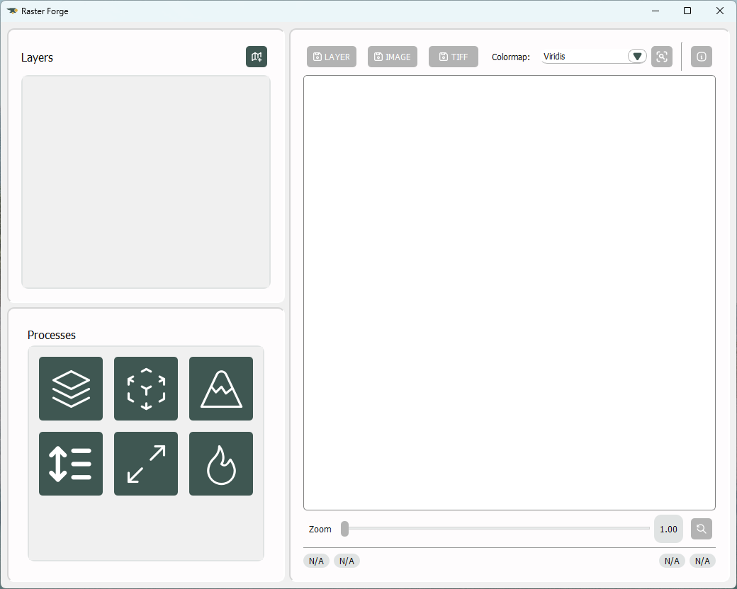
Figure 2: The GUI is arranged into three distinct panels: the layers panel located at the top-left, the processes panel positioned at the bottom-left, and the viewer panel situated on the right.

To simplify importing data, a dedicated window has been designed to enable users to select a file, as depicted in Figure 3. Within this window, users can preview the file’s composition, including the number of bands it contains. Users can select bands to import and specify the desired scale. Additionally, the window displays the predicted width and height of the resulting array, aiding users in assessing the computational resources required for any further processing.

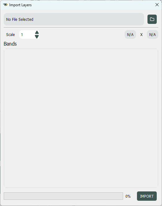
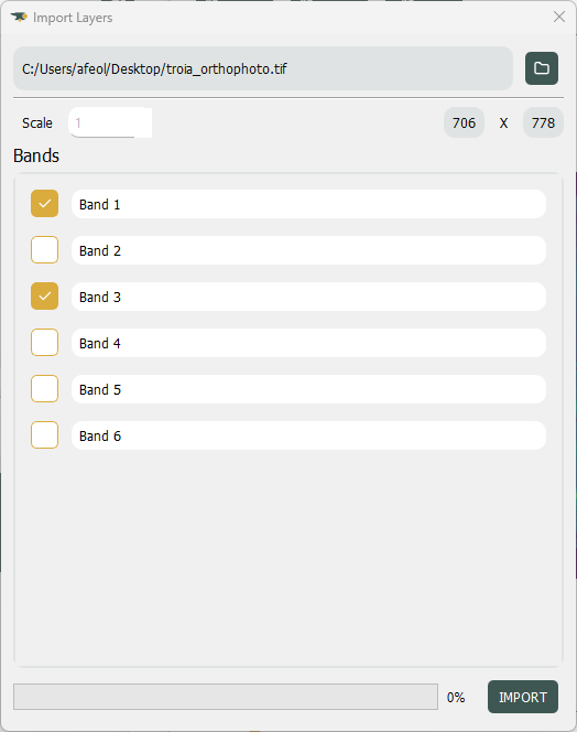
(a)	(b)

Figure 3: Layer import panel showcasing its initial state (a) and after selection of a file (b). The predicted values for width and height dynamically adjust based on the chosen scale.

After the layers are imported, they are displayed on the Layer list, as depicted in Figure 4. Each layer offers four distinct functionalities: viewing the layer, editing the layer identifier, accessing layer information, and deleting the layer. Layer information is presented in an information window (see Figure 5) consisting of three tabs: metadata, statistical data, and a value histogram.

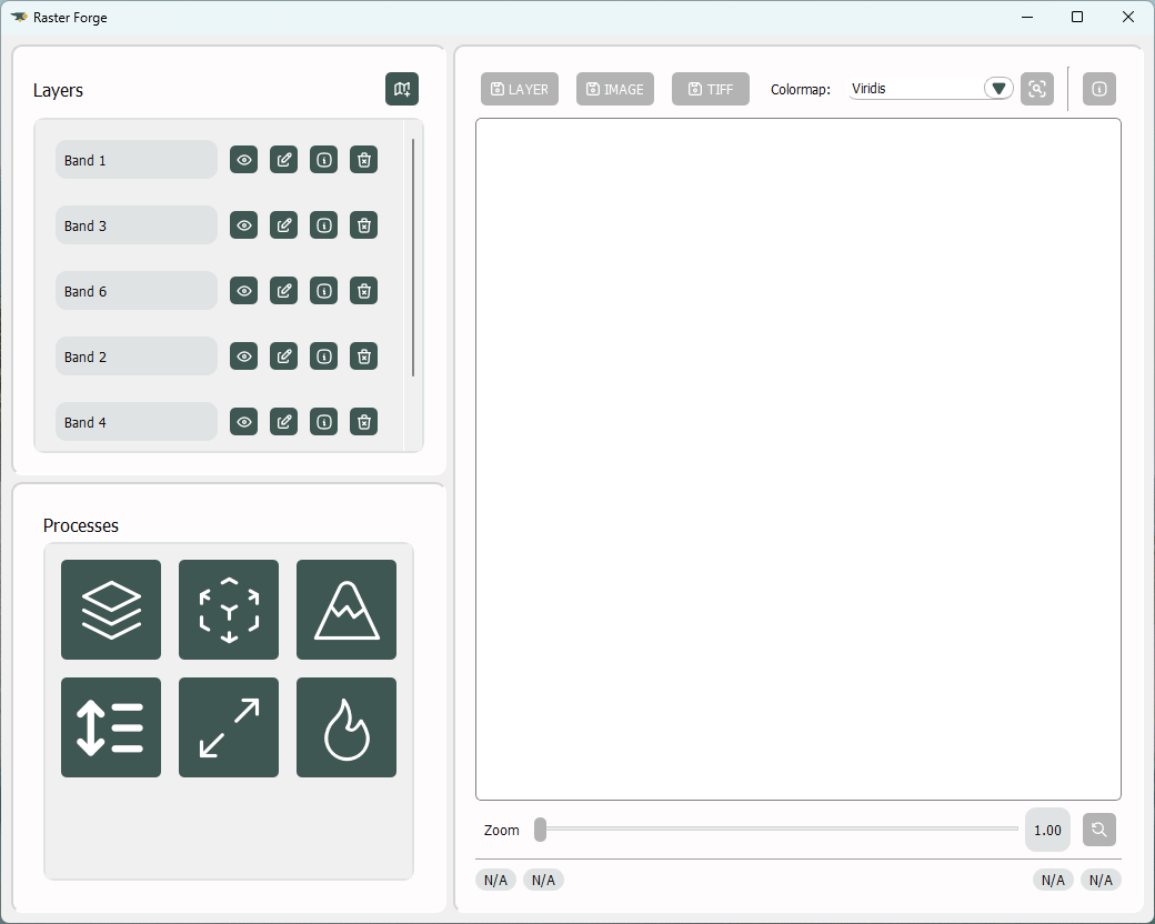
Figure 4: Upon importing layers, the graphical user interface (GUI) offers access to layer functionalities. For each layer, four functionalities are available, namely: view layer, edit layer’s name, access layer information, and delete layer.

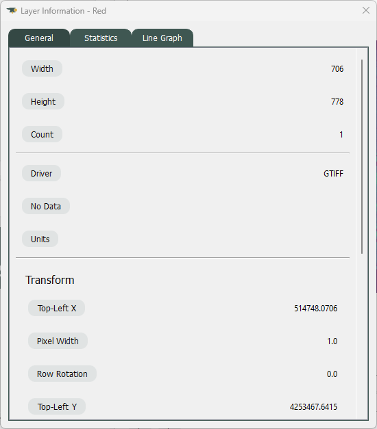
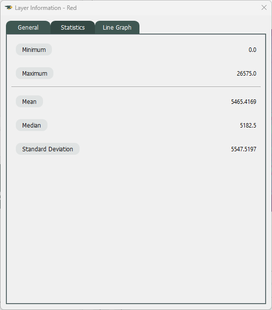
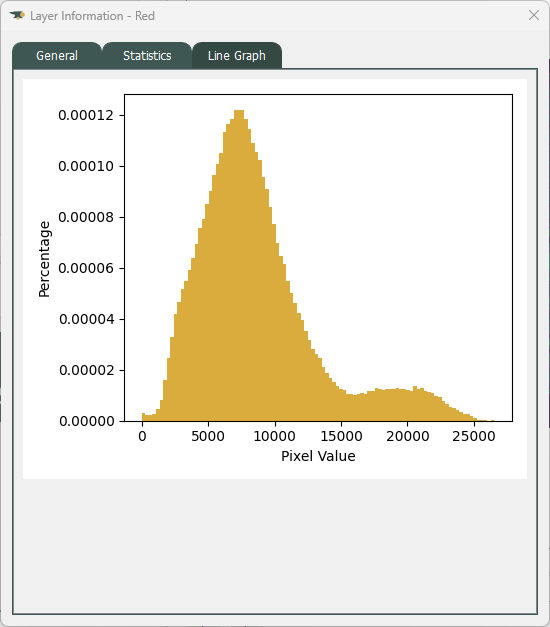
(a)	(b)	(c)

Figure 5: Layer information panel composed of three tabs: metadata, statistical insights, and value histogram.

Once the layers are loaded, they can be used in various processes. All processing functions in the library are accessible through the GUI. When selecting a process, an adaptive panel displays all necessary inputs. The process can be initiated once all inputs are fulfilled, as shown in Figure 6. Once activated, the data is displayed on the viewer and can be saved in various formats: as a layer for reuse in other processes, as an image with the applied colormap, or as a raw TIFF file containing all geographical information of the area. The information window for the currently viewed data is available directly on the viewer panel, even if it has not been saved as a layer yet.

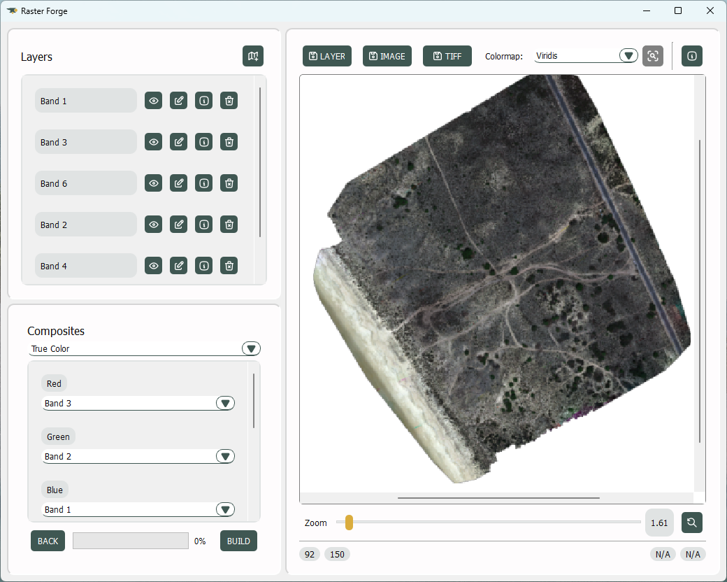
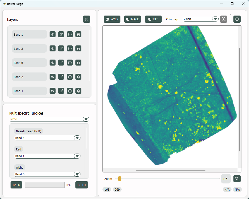
(a)	(b)

Figure 6: Creating a (a) true color composite, and a (b) multispectral index map. The adaptive panel inputs are located within the processes panel, alongside the functionalities accessible within the view panel once an image is being viewed. These include zoom options, colormap selection, and various saving actions

   3.     Impact

Raster manipulation software is used in a wide range of applications and fields, including medical imaging [23, 24], architecture [25, 26], and planetary [27, 28] and interplanetary [29, 30] remote sensing. However, as can be seen from the importance given to the geographical aspect of each raster, Raster Forge has been designed and developed with a primary focus on the field of remote sensing, and more specifically where it intersects with wildfire management.

Raster Forge was used to compute feature maps for an area of interest [31], including vegetation coverage, water, and man-made structures. The software also generated slope and aspect maps, which are crucial for calculating wildfire spread and growth. Additionally, a canopy height map was produced, providing an indication of fuel density in a specific region. Finally, Raster Forge allowed for the creation of complete fuel maps that are ready and easy to integrate into wildfire simulation environments, such as FlamMap [32], to predict the fire risk in a particular area.

Out of the particular focus of wildfire management, Raster Forge can have many other applications. The ability to extract water body maps and analyze ground moisture content can be very helpfully in hydrological modeling. Additionally, the software enables users to quickly assess the same area across various multispectral indices, which is particularly useful for gauging vegetation health, a critical aspect of agricultural endeavors.

   4.     Conclusions

In conclusion, Raster Forge provides a solution for manipulating raster data, specifically designed for remote sensing applications such as wildfire management. The Raster Forge library offers a range of functions for raster processing, including composite generation, multispectral index computation, topographical feature extraction, and fuel map creation. Its included GUI is user-friendly, streamlines the use of the functionalities of the library and simplifies data import, layer management, process configuration, and result visualization. This enhances accessibility for users with varying levels of expertise. Raster Forge has potential applications in diverse fields such as disaster management, hydrological modeling, agriculture, and environmental monitoring, positioning itself as a valuable tool for geospatial data analysis and visualization tasks.

   Funding

This work was financed by the Portuguese Agency FCT (Fundação para a Ciência e Tecnologia), in the framework of projects UIDB/00066/2020, UIDB/04111/2020 and CEECINST/00147/2018/CP1498/CT0015.

References

- [1] Milan Sonka, Vaclav Hlavac, and Roger Boyle. Image processing, analysis and machine vision. Springer, 2013.
- [2] C Gonzalez Rafael and E Woods Richard. Digital image processing. Pearson education, 2018.
- [3] Mengna Li, Youmin Zhang, Lingxia Mu, Jing Xin, Ziquan Yu, Shangbin Jiao, Han Liu, Guo Xie, and Yi Yingmin. A real-time fire segmentation method based on a deep learning approach. IFAC-PapersOnLine, 55(6):145–150, 2022.
- [4] Xijiang Chen, Qing An, and Kegen Yu. Fire identification based on improved multi feature fusion of ycbcr and regional growth. Expert Systems with Applications, 241:122661, 2024.
- [5] Guodong Wang, Di Bai, Haifeng Lin, Hongping Zhou, and Jingjing Qian. Firevitnet: A hybrid model integrating vit and cnns for forest fire segmentation. Computers and Electronics in Agriculture, 218:108722, 2024.
- [6] Ning Wang, Shiyue Zhao, and Sutong Wang. A novel clustering-based resampling with cost-sensitive boosting method to model and map wildfire susceptibility. Reliability Engineering & System Safety, 242:109742, 2024.
- [7] LA Sanabria, X Qin, J Li, RP Cechet, and Christopher Lucas. Spatial interpolation of mcarthur’s forest fire danger index across australia: observational study. Environmental modelling & software, 50:37–50, 2013.
- [8] Michael F Goodchild. Geographic information systems and science: today and tomorrow. Annals of GIS, 15(1):3–9, 2009.
- [9] GDAL/OGR contributors. GDAL/OGR Geospatial Data Abstraction software Library. Open Source Geospatial Foundation, 2024.
- [10] Sean Gillies et al. Rasterio: geospatial raster i/o for Python programmers, 2013–.
- [11] G. Bradski. The OpenCV Library. Dr. Dobb’s Journal of Software Tools, 2000.
- [12] Markus Neteler, M Hamish Bowman, Martin Landa, and Markus Metz. Grass gis: A multi-purpose open source gis. Environmental Modelling & Software, 31:124–130, 2012.
- [13] CA: Environmental Systems Research Institute Redlands. Arcgis desktop: Release 10, 2011.
- [14] QGIS Development Team. QGIS Geographic Information System. QGIS Association,
- [15] Sean Gillies et al. Rasterio. https://github.com/rasterio/rasterio, 2024. Accessed: April 4th of 2024.
- [16] Qt Project. PySide Logo, 2023. Accessed: April 4th of 2024.
- [17] NumPy Contributors. NumPy Logo, 2020. Accessed: April 4th of 2024.
- [18] David Montero Loaiza et al. Awesome Spectral Indices in Python. https://github.com/awesome-spectral-indices/spyndex, 2024. Accessed: April 4th of 2024.
- [19] OpenCV Development Team. OpenCV Media Kit, 2024. Accessed: April 4th of 2024.
- [20] Charles R. Harris, K. Jarrod Millman, Stéfan J. van der Walt, Ralf Gommers, Pauli Virtanen, David Cournapeau, Eric Wieser, Julian Taylor, Sebastian Berg, Nathaniel J. Smith, Robert Kern, Matti Picus, Stephan Hoyer, Marten H. van Kerkwijk, Matthew Brett, Allan Haldane, Jaime Fernández del Río, Mark Wiebe, Pearu Peterson, Pierre Gérard-Marchant, Kevin Sheppard, Tyler Reddy, Warren Weckesser, Hameer Abbasi, Christoph Gohlke, and Travis E. Oliphant. Array programming with NumPy. Nature, 585(7825):357–362, September 2020.
- [21] David Montero, César Aybar, Miguel D Mahecha, Francesco Martinuzzi, Maximilian Söchting, and Sebastian Wieneke. A standardized catalogue of spectral indices to advance the use of remote sensing in earth system research. Scientific Data, 10(1):197, 2023.
- [22] Pyside6.
- [23] Jahanzaib Latif, Chuangbai Xiao, Azhar Imran, and Shanshan Tu. Medical imaging using machine learning and deep learning algorithms: a review. In 2019 2nd International conference on computing, mathematics and engineering technologies (iCoMET), pages 1–5. IEEE, 2019.
- [24] Sandra Jardim, João António, and Carlos Mora. Image thresholding approaches for medical image segmentation-short literature review. Procedia Computer Science, 219:1485–1492, 2023.
- [25] M Quamer Nasim, Narendra Patwardhan, Tannistha Maiti, Stefano Marrone, and Tarry Singh. Veernet: Using deep neural networks for curve classification and digitization of raster well-log images. Journal of Imaging, 9(7):136, 2023.
- [26] Han Tu, Yichao Shi, and Meng Xu. Integrating conditional shape embedding with generative adversarial network-to assess raster format architectural sketch. In 2023 Annual Modeling and Simulation Conference (ANNSIM), pages 560–571. IEEE, 2023.
- [27] Fei Li, Tan Yigitcanlar, Madhav Nepal, Kien Nguyen, and Fatih Dur. Machine learning and remote sensing integration for leveraging urban sustainability: A review and framework. Sustainable Cities and Society, page 104653, 2023.
- [28] Sha Huang, Lina Tang, Joseph P Hupy, Yang Wang, and Guofan Shao. A commentary review on the use of normalized difference vegetation index (ndvi) in the era of popular remote sensing. Journal of Forestry Research, 32(1):1–6, 2021.
- [29] WANG Tao, WANG Gangyi, WEI Xinguo, and LI Yongyong. A star identification algorithm for rolling shutter exposure based on hough transform. Chinese Journal of Aeronautics, 2023.
- [30] Zhenduo Zhang, Wenbo Zheng, Zhanjun Ma, Limei Yin, Ming Xie, and Yuanhao Wu. Infrared star image denoising using regions with deep reinforcement learning. Infrared Physics & Technology, 117:103819, 2021.
- [31] Afonso Oliveira, Nuno Fachada, and João P. Matos-Carvalho. Data science for geographic information systems, 2024.
- [32] Mark A. Finney, Stacey Brittain, Rob C. Seli, Charles W. McHugh, and Louis Gangi. FlamMap: Fire mapping and analysis system (version 6.2), 2023.