Maximum Degree in Random Hyperbolic Graphs
Abstract
The random hyperbolic graph, introduced in 2010 by Krioukov, Papadopoulos, Kitsak, Vahdat and Boguñá [12], is a graph model suitable for modelling a large class of real-world networks, known as complex networks. Gugelmann, Panagiotou and Peter [11] proved that for curvature parameter , the degree sequence of the random hyperbolic graph follows a power-law distribution with controllable exponent up to the maximum degree. To achieve this, they showed, among other results, that with high probability, the maximum degree is , where is the number of nodes. In this paper, we refine this estimate of the maximum degree, and we extend it to the case : we first show that, with high probability, the node with the maximum degree is eventually the one that is the closest to the origin of the underlying hyperbolic space (Theorem 3.1). From this, we get the convergence in distribution of the renormalised maximum degree (Theorem 3.2). Except for the critical case , the limit distribution belongs to the extreme value distribution family (Weibull distribution in the case and Fréchet distribution in the case ).
MSC2020 subject classifications: 05C80, 05C07, 60G70.
Key words: random hyperbolic graphs, maximum degree, generalised extreme value distribution.
1 Introduction
The study of real-world networks requires constructing different mathematical models to encompass all possible behaviours of these networks. One of the most natural models we have for studying real-world networks is the random geometric graph model. This graph model was first introduced by Gilbert [10]; its particularity lies in the utilization of an underlying geometric space: a random geometric graph is constructed by choosing nodes at random in a bounded domain of , and connecting every pair of nodes separated by a distance smaller than a certain threshold [14].
When studying connectivity in random graphs, the maximum degree is a significant quantity to consider, because nodes with high degree act as hubs that connect many nodes together. The maximum degree also plays an important role in the so-called small world property. Indeed, the existence of very large hubs allows for finding short paths between pairs of nodes by travelling from hub to hub. In the random geometric graph model, we have a good understanding of the asymptotic behaviour of the maximum degree for various regimes in . Studying the maximum degree in these graphs requires adapting some classical mathematical tools to this framework. The most important ones are the Poisson approximation and the dependency graphs. For instance, these tools are used to show that there exists a whole class of regimes in which the maximum degree asymptotically concentrates on two values as goes to infinity, see [14, Theorem 6.3 and 6.6].
Although random geometric graphs seem natural for modelling purposes, they fail to capture a class of real-world networks known as complex networks. This class comprises large graphs that primarily arise from human interactions such as social networks and the Internet, as well as from other fields like biology (we recommend the review by Albert and Barabási on the topic [2]). Networks in this class exhibit four essential features: high clustering, the small world property, sparseness and a scale-free degree distribution [7]. Krioukov, Papadopoulos, Kitsak, Vahdat and Boguñá [12] showed that these four properties naturally emerge in graphs constructed on the hyperbolic space. They introduced the random hyperbolic graph (also denoted RHG), and they empirically showed that this graph can model complex networks. Boguñá, Papadopoulos and Krioukov further illustrated this point by providing an embedding of the Internet graph into the hyperbolic space [5]. For modelling purposes, the model can be tuned through a curvature parameter and a parameter that fixes the average degree.
It has now been rigorously proven that, in the regime , the random hyperbolic graph exhibits all the properties of complex networks listed above. Sparseness is proven in [15, Theorem 6.4], the small world property is shown in [1] and the high clustering is also fully tested [6, 9, 11]. Finally, the scale-free degree distribution of RHG has been proven up to the maximum degree in [11]. It is also shown in [11] that, for curvature parameter , the maximum degree of the RHG is with high probability , where is the number of nodes. The Poisson approximation method developed for studying the maximum degree in the Euclidean setting [14, Theorem 3.4] cannot be used to prove this estimation on the maximum degree. Indeed, in the Euclidean setting, no point of the underlying space is privileged in terms of connectivity (the boundary effects vanish in the limit), explaining the efficiency of the Poisson approximation in counting the number of nodes with a certain degree. However, in RHGs, the expected value of the degree of a given node decreases rapidly as the node moves away from the origin of the underlying space, leading to a completely different behaviour. Nevertheless, this particularity of RHGs is used in [11] to show that the node with the highest degree is, with high probability, one of the nodes closest to the origin. The estimation of the maximum degree obtained in [11] follows from this observation.
The case is referred to as the dense regime because the RHG is not sparse in this case. We also observe a threshold for connectivity at : for , the graph has a high probability of being connected and the connection is entirely ensured by a few large hubs located near the centre. Conversely, for , the graph has a high probability of being disconnected. In the critical phase , the probability of connectivity tends to a constant that depends on the parameter . This constant takes the value if and only if (see [4]).
Our results. In this paper, we refine the estimation of the maximum degree in the regime , given in [11]. We also extend the study of the maximum degree to the case . To achieve this, we first show that, for any value of , the highest degree is eventually attained by the node that is the closest to the origin of the underlying space (Theorem 3.1). Then we compute the distribution of the degree of this node to get the convergence in distribution of the renormalised maximum degree (Theorem 3.2). The maximum degree heavily depends on the curvature parameter . As with connectivity, a phase transition occurs at : for , the maximum degree is of order , whereas for , the maximum degree is of order .
The limit distributions obtained in the regimes and belong to the family of extreme value distributions. Hence, in these cases, the maximum degree satisfies the conclusion of the extreme value theorem (see [13]). However, the premises of this theorem are not verified here, as the degrees of the nodes are not independent. One may think of using an extension of this theorem for stationary sequences (see, for example, [13, Theorem 2.1.2]), though it is unclear whether the degree sequence satisfies the strong mixing property required for this theorem to apply.
The fact that the maximum degree is attained by the closest node to the origin is natural, as the degree of this node stochastically dominates the degree of the other nodes. However, this observation alone is insufficient to conclude, as this one node has to compete against the other nodes. For instance, for the celebrated tree model known as the random recursive tree, Devroye and Lu [8] demonstrated that, with high probability, the maximum degree is , whereas the degree of the root is only . Thus, with high probability, the degree of the root is much smaller than the maximum degree, even though, in this tree model, the degree law of the root dominates the degree law of each of the other nodes. In our study of RHGs, we show that, with high probability, the closest node to the origin is sufficiently close to the origin, in comparison with the other nodes (see Proposition 5.2), in order to compete with the other nodes.
The study of the degree in RHGs primarily relies on the computation of the measures of certain regions of the underlying hyperbolic space. The exact expressions of these measures are seldom tractable, but since we are seeking asymptotic results, we only need to approximate these quantities. The approximations we employ depend on the value of the curvature parameter , as the position of the closest node to the origin depends on this parameter. In the regime we can make use of the approximations from [11, Lemma 3.2] (see Lemma 4.3 of this paper). In the two regimes and , we require new approximations (given by Lemmas 4.4 and 4.5 respectively).
Structure of the paper. In Section 2, we recall some basic facts about hyperbolic geometry and the definition of the random hyperbolic graph. Our main results (Theorems 3.1 and 3.2) are presented in Section 3, along with a sketch of their proofs. Section 4 is dedicated to the computation of the measure of important regions of the underlying hyperbolic space. In Section 5, we state some convergence in distribution results to precisely locate the closest node to the origin and to show that the other nodes are not too close to the origin. Finally, in Sections 6 and 7, we use the results from the previous two sections to prove Theorems 3.1 and 3.2.
2 Definition of the model
2.1 Hyperbolic geometry
Before introducing the random hyperbolic graph model, let us review some definitions and notations concerning hyperbolic geometry. We refer to the book of Stillwell [16] for a broader introduction to hyperbolic geometry. The Poincaré disk, denoted by , is the open unit disk of equipped with the Riemannian metric defined at by
We denote by the distance induced by on . Throughout this paper, we make extensive use of the polar coordinates to describe points in the Poincaré disk. The polar coordinates of a point in represent its hyperbolic distance to the origin () and its angle in the complex plane (). The quantity is also referred to as the radius of . Unless mentioned otherwise, each figure is represented after the function
is applied. This corresponds to dilating each distance to the origin so that each point is represented with a Euclidean distance to the origin equal to its radial coordinate . This representation of is known as the native representation and has previously been used in [12] for visualisation purposes.
For coordinates of a point in and , we denote by the open hyperbolic ball of radius centred at . We write the ball of radius centred at . For , we define as the annulus with inner radius and outer radius , i.e., . Finally, for two points and in with respective polar coordinates and , the hyperbolic distance between and is given by the celebrated hyperbolic law of cosines:
| (1) |
2.2 The Random Hyperbolic Graph
Let us now proceed to the formal definition of the random hyperbolic graph . We fix two parameters and , and for all , we set
| (2) |
We can construct a probability measure on , such that if the point (in polar coordinates) is chosen according to , then and are independent, is uniformly distributed in and the probability distribution of r has a density function on given by
| (3) |
Finally, we define the set by
where the are independent and identically distributed random variables with distribution given by . We denote by the random hyperbolic graph with nodes and parameters and . It is defined as the undirected graph whose nodes are the points of and in which two nodes are connected by an edge if and only if they are at a hyperbolic distance of at most from each other. We also define the random variable as the point of that is the closest to the origin of , i.e.,
where is the smallest index that minimises the quantity . The degree of a node of the graph is defined as its number of direct neighbours in the graph . It is sometimes denoted .
Observe that the nodes of the graph are located within . Also, note that the value of is considered large, as all our results hold for , while and are fixed. The measure of a ball centred at is independent of . Therefore, we omit the angle whenever we can to shorten notations. Thus, we rather write . Likewise, we write instead of .
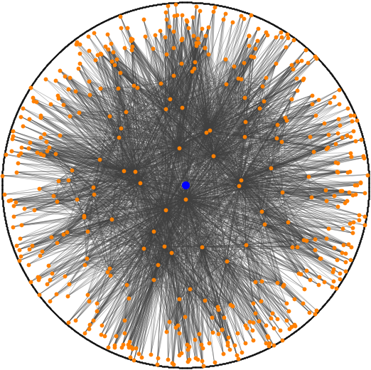
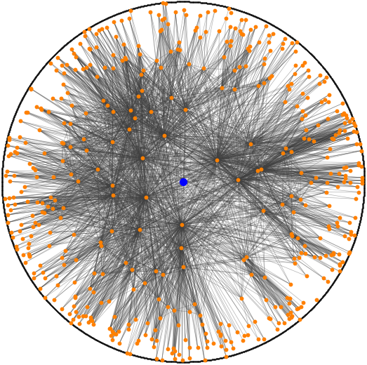
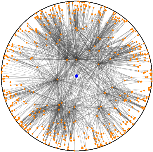
In the special case , is the uniform measure on associated with the Riemannian metric . In the general case, corresponds to a uniform measure on the hyperbolic plane of curvature . More precisely, for fixed , we can multiply the differential form in the Poincaré disk model by a factor to obtain a hyperbolic plane of curvature . Choosing a point according to the measure amounts to choosing a point uniformly in the ball of radius of and projecting it on , by keeping the same polar coordinates. A simple computation shows that the measure of a ball of radius in is given by
therefore, the bigger is, the faster it increases with . Therefore, the bigger is, the more points of the graph concentrate near the boundary of . So, the maximum degree is expected to increase with (see the simulations in Figure 1).
Landau’s notations: We use the Landau notations and to describe the limit behaviour of certain quantities as the number of nodes goes to infinity. Specifically, we use a version of these notations that allows us to express uniformity in some other variables . Namely, for a sequence of subsets of and two functions , we write
| (4) |
and we write
| (5) |
Note that the subscript "" indicates that the comparison holds uniformly for in the set as goes to infinity. To simplify notations, this subscript is specified beforehand and dropped from the notations in most cases. When and are functions of the variable only, we keep the same definitions but remove the "".
3 Results and sketch of proofs
The sequel of this paper is dedicated to proving the following results about the maximum degree.
Theorem 3.1.
For fixed and , consider the graph . Let denote the degree of the closest node to the origin and let denote the maximum degree among all other nodes. Then,
Theorem 3.2.
The probability density functions of the limit distributions appearing in Theorem 3.2 can be retrieved from the characteristic functions appearing at the end of the proof of this result (see Section 7).
Let us outline the main ideas of the proofs of Theorem 3.1 and Theorem 3.2. The key point is to locate in a certain annulus and show that the radii of the other nodes are not too close to the radius of . In order to do so, we define the following sequences that appear throughout the paper. In the case , there is no need for such sequences.
Definition 3.3.
Let be a sequence of real numbers such that:
Using this sequence, we define three other sequences , and , given in the following table. Their definitions depend on the value of .
We also define
We denote by the difference between the radius of the second closest node to the origin and the radius of . We call it the radius gap. The role of the variable is crucial to the proof of Theorem 3.1. Indeed, we can compute the rate at which the expected degree of a given node decreases when the radius of this node increases. Thus, the variable provides information about the difference between the expected degree of and the expected degree of the other nodes.
Propositions 5.1 and 5.2 from Section 5 are key results that give the convergence in distribution of the variables and (renormalised). For instance, they directly imply the following lemma, which also provides an interpretation of the sequences defined in Definition 3.3. The interval appears to be the domain in which concentrates and is a lower bound for , which holds with high probability. The proof of this lemma is postponed until the end of Section 5.
Lemma 3.4.
For ,
and
Thus, in the case , the minimal node radius is of order , while in the case , the minimal node radius is of order . However, in the critical regime , the minimal node radius (without renormalisation) converges in distribution (see Proposition 5.1). Consequently, localising the node is easier in this case, making the critical regime simpler to study. Therefore, we provide fewer details when proving our results in the regime and rather focus on the other two regimes. In many proofs, the three different regimes in are treated separately, but the general idea remains the same in all cases.
The main steps of the proof of Theorem 3.1 (see Section 6 for a complete proof) are as follows: we know by Lemma 3.4 that it suffices to prove the following convergence
| (6) |
where the event is defined by
We denote by the points of and we denote the cardinality of any set as . Using a simple union bound, we obtain the following upper bound
Since a node located at is connected to all the nodes in , it also holds that
Finally, on the event , the approximations provided in Section 4 allow us to show that is much larger than . Combining these approximations with Chernoff bounds yields two positive constants and independent of such that
These three relations together prove the convergence at (6), thereby establishing Theorem 3.1.
Instead of directly proving Theorem 3.2, we rather prove the same statement with replaced by . By Theorem 3.1, this is sufficient to establish Theorem 3.2. To achieve this, we observe that, conditionally on the position of the node , the other nodes are uniformly chosen in the annulus (see Figure 2). Moreover, the node is connected to all the nodes in the green region . So, conditionally on , the variable follows a binomial distribution with trials and probability
(see Figure 2). Using the estimates of obtained in Proposition 5.1 and the measure estimations provided in Section 4, we can estimate . The conclusion follows from a direct computation of the characteristic function of (see Section 7 for a complete proof).
Open question. Let us conclude this section with an open question concerning Theorem 3.1. Our proof of Theorem 3.1 can be extended to prove the following result: for a fixed integer , the ranking of the nodes by increasing radii coincides with the ranking by decreasing degree up to rank , with high probability. What happens if we let evolve with ? In other words, up to what rank do the two rankings coincide?
4 Measures of balls and differences of balls
In this section, we present some results concerning the measures of certain domains of the underlying hyperbolic space. Since we are principally concerned with the asymptotic behaviour of , we prefer to provide approximations of these quantities rather than exact expressions. It’s important to note that some of the quantities studied in this section cannot be expressed by a tractable closed-form formula.
Let us first focus on the measure of hyperbolic balls centred at the origin. The two following approximations follow directly from integrating the density function . These approximations are used in the next section to localise the minimum radius . Recall that we use a slightly modified version of Landau’s notations and (see (4) and (5)).
Lemma 4.1.
Let us fix and a sequence that converges to infinity.
For , we have
| (7) |
For , we have
| (8) |
In the remaining part of this section, we focus on balls that are no longer centred at the origin. This is more involved because such balls intersect the complement of the domain (see Figure 2). Degrees in RHGs are closely related to the measures of these balls, and more generally to the measures of differences of balls, e.g., the expected degree of a node of radius is .
Before dealing with quantitative results, we state the following lemma, which gives an intuitive inclusion between hyperbolic balls. Its proof follows readily from [3, Lemma 2.3]. The decreasing of in obtained here shows that the expected degree of a node is a decreasing function of . This is a strong clue to the fact that the highest degree node is to be found next to the origin of the underlying space.
Lemma 4.2.
For all , and , the following holds
In particular, the application is decreasing.
Since we are interested in the degree of , we need an approximation of for values of in a certain interval that contains with high probability. To obtain this, we first give an integral expression of . In the following definitions, we take , and we fix an integer . We also take and in . Let us define the set by
A direct use of the hyperbolic law of cosines (1) yields that is a non-empty interval. So defining by
we get
| (9) |
Figure 3 below provides a graphical representation of the angle (in a Euclidean setting to ease the representation). Let us fix . We want to compute for . It is clear that , so
| (10) |
When , the point is at a distance from the point , so by the hyperbolic law of cosines (1), we get
| (11) |
One may check that equations (10) and (11) can be rewritten as:
| (12) |
We are now ready to present estimations of for values of corresponding to the typical values taken by . Since the asymptotic behaviour of depends on the value of , we shall make different computations in the three different regimes.
In the case , we make direct use of the estimates from [11, Lemma 3.2], which follow (in a non-trivial way) from approximating (9). The following lemma is a weaker but more convenient version of [11, Lemma 3.2]. Recall that the sequences and are defined in Definition 3.3.
Lemma 4.3.
Suppose , set and fix . For and , we have,
| (13) | ||||
| (14) |
Proof.
Formula (13) follows directly from (8). In the following proof of (14), all Landau’s terms ( and ) are uniform over and . We distinguish between two cases. In the case , by [11, Lemma 3.2], we have
In the case , it holds that
Since and , it follows from [11, Lemma 3.2] that
As in the previous case, we can show that the error term is , completing the proof of (14). ∎
In the case , we give the following approximation of . This approximation is valid for in the interval , which contains with high probability. As goes to infinity, the bounds of this interval quickly approach . Therefore, it is not surprising that tends to as goes to infinity. Here we provide additional information regarding the rate at which this quantity decreases with .
Lemma 4.4.
Let us fix . For , we have
Proof.
For all , we define by
| (15) |
Now, to find a good approximation of , we use (11). The two bounds of the interval go to as goes to . So approximating all the hyperbolic terms in of the identity given at (11) yields, for and ,
| (16) |
Moreover, it holds that
So using , we get, for and ,
| (17) |
Combining (16) with (17) yields, for and ,
| (18) |
For , we define
| (19) |
Let us show that is a good approximation of . Since is -Hölder, it follows from (18) that, for and for ,
Combining this estimate of with (15) yields, for ,
| (20) |
Now, it remains to estimate . Let and . Integrating (19) by parts gives
Furthermore, the mean value theorem yields, for and ,
so
Combining this with (4) yields,
∎
In the case , the minimal node radius (without renormalisation) converges in distribution (see Proposition 5.1), thus we need to approximate for fixed . This is the purpose of the following lemma. This result is stated for every possible value of , as this comes without extra cost.
Lemma 4.5.
Suppose is fixed. Then, for every ,
where is a strictly decreasing diffeomorphism from to defined by:
| (21) |
Proof.
Let us fix and . For all and , we define as the only positive real number such that
| (22) |
The change of variable , in the expression of given at (9), yields
| (23) |
Let us fix . By the definition of given at (22), we have
Combining this with the expression of given at (12) yields
Thus, the convergence of follows from applying the dominated convergence theorem to (23). The fact that is a strictly decreasing diffeomorphism from to follows directly from its expression given at (21). ∎
5 Convergence in distribution of the minimal node radius and the radius gap
In this section, we prove the convergence in distribution of the variables and (renormalised). Recall that the variables and are defined in Sections 2.2 and 3 respectively. To prove the convergence of the variable (renormalised), we rely on Scheffé’s lemma, as it also provides the convergence of the corresponding density function. This convergence is quite useful for subsequently stating convergence in distribution results for and .
Before delving into the computations, let us define a more convenient way of sampling the nodes of the graph . We note that the density function of the polar coordinates of the node is given by:
| (26) |
where is defined by
| (27) |
Thus, instead of independently sampling the points in according to the measure , we can choose with density , and then choose the other points according to the measure restricted to the annulus . This equivalent way of sampling the nodes of the graph is very convenient for our purposes, as it focuses on the node .
We aim to precisely locate the node by establishing a convergence in distribution of a renormalised version of . Before proceeding further, we present the following definitions and remarks, which follow from straightforward changes of variables in the density :
In the regime , is a continuous random variable, with density defined on by:
| (28) |
In the regime , is a continuous random variable, with density defined on by:
| (29) |
In the regime , is a continuous random variable, with density defined on by:
| (30) |
The following proposition shows that the manner in which is renormalised above is the correct way to ensure convergence.
Proposition 5.1.
Convergence in distribution of the renormalised minimum radius:
The sequence of density functions converges in to the function defined on by:
| (31) |
In particular,
| (32) | ||||
| (33) | ||||
| (34) |
Proof.
We treat the three regimes separately.
In the regime :
Fix . By (27) and (28), we get, for ,
Thus, for large enough, we obtain from the expression of given at (3),
Furthermore, the approximation of given at (7) yields
So, we finally get
The conclusion follows from Scheffé’s lemma.
In the regime :
Fix . Proceeding as in the previous case, we get, for large enough,
so using and (8), we obtain
We conclude with Scheffé’s lemma once again.
The proof of the case is similar. ∎
The following result is the analogous of Proposition 5.1 for the radius gap .
Proposition 5.2.
Proof.
We make separated computations for the three regimes in .
In the regime :
Fix . Using the sampling of the nodes described at the beginning of this section and integrating over the value of , we get
By the change of variable , we deduce that
(35) where is the function defined at (28) and is the function defined on by
(36) We now use the convergence in stated in Proposition 5.1 to compute the limit of the integral at (35). Fix . For sufficiently large , we have
(37) Moreover, a straightforward computation using (7) gives that
(38) Inserting (37) and (38) into (36) yields
(39) On the other hand, for all , it is clear that
(40) Since converges toward in , as stated in Proposition 5.1, we deduce from (39) and (40) that
where the function is defined on by
Notice that is continuous and decreasing. Moreover, it holds that
So the variable converges in distribution and the limit has cumulative distribution function defined by
(41) where is the complementary error function.
In the regime :
Fix . Proceeding as in the previous case, we get
By the change of variable , we deduce:
(42) where is the function defined at (30) and is the function defined on by
(43) Fix . For large enough, we have
(44) And a simple computation using (8) gives
So combining (43) with (44), we get
(45) On the other hand, for all , it is clear that
(46) Since converges toward in , as stated in Proposition 5.1 , we deduce from (45) and (46) that
So, by (42), we obtain
In the regime :
The proof for this case is very similar to the previous cases. The cumulative distribution function of the limit distribution is given by:
(47)
∎
6 Proof of Theorem 3.1
We know that the closest node to the origin has the highest expected degree. Therefore, to prove Theorem 3.1, we can use our previous results on and together with the estimates from Lemmas 4.3 and 4.4, to show that the expected degrees of the other nodes are sufficiently small compared to the expected degree of the closest node to the origin. The following lemma relies on Chernoff’s bounds. It provides a way to translate this information into a bound on the probability that one of these nodes has a higher degree than the closest node to the origin. Note that this result does not require the two variables and to be independent. Thus and may be legitimately replaced by and the degree of any other node, as it is done in the proof of Theorem 3.1, which follows below. In the following, we denote by the binomial distribution with parameters and .
Lemma 6.1.
Let and . If , then
Proof.
By splitting at , we get
Recall that, for and , the multiplicative Chernoff bounds are as follows:
Since and , we can use these bounds to obtain
which proves our claim. ∎
We are now ready to prove Theorem 3.1.
Proof of Theorem 3.1.
Let us start with the case . By Lemma 3.4, it suffices to show that
We denote by the points of and we define
We also define the set by
The probability of interest can be rewritten as
Thus, by a union bound, we have
So, conditioning on , we finally get
| (48) |
Note that if is connected to in the graph , then is also connected to . Thus, this connection does not contribute to the inequality . Therefore, for the remainder of the proof, we redefine (resp. ) as the number of neighbours of (resp. ) in instead of . Having taken this extra care, we can show (see Figure 4) that, conditionally on , the variable is distributed as:
| (49) |
and the variable is distributed as:
| (50) |
In the remaining part of the proof of the case , we compare the terms and defined above, when is taken in . We then use Lemma 6.1 to conclude. This remaining part depends on the value of . Let us also mention that the constant stands for a positive constant whose value depends only on and and can change along the proof.
In the regime :
Let us take and . Since is decreasing (see Lemma 4.2), it follows that
Since and are in , we can use Lemma 4.4 and (7) to deduce that
(51) From this, we get, for large enough,
(52) It also gives
(53) The two inequalities (52) and (6) allow us to use Lemma 6.1 together with the conditional distributions given at (49) and (50) to assert that, on the event , we have
Combining this with (6) yields
which concludes the proof of this case.
In the regime :
Let , we verify that for sufficiently large , we have for all :
Thus, by (13) and (14) we get, for ,
(54) Likewise, using also the monotonicity of (Lemma 4.2), we get, for ,
(55) Hence, for ,
So, for sufficiently large, we get
(56) The estimates given at (54) and (55) also imply, for ,
Since , we finally obtain
(57) The two inequalities (56) and (57) allow us to use Lemma 6.1 together with the conditional distributions given at (49) and (50) to assert that, on the event , we have
We conclude as in the previous case.
Now, let us proceed with the case . We take and for all , we introduce the following set:
where is the function defined in Lemma 4.5. Since the function is strictly decreasing, we find that, for every , the set covers all of . So, by the convergences in distribution proven in Proposition 5.1 and Proposition 5.2, we can fix , , such that
Thus, it remains to prove that
| (58) |
Let us define the set by
Proceeding as in the proof of (6), we prove that
| (59) |
The functions are decreasing in and the point-wise limit is continuous. So, the convergence proven in Lemma 4.5 is uniform on the compact interval . So, for sufficiently large, we get
Using this inequality, we can proceed as in the case to show that, on the event , we have
Combining this with (6) proves the limit at (58), which concludes the proof. ∎
7 Proof of Theorem 3.2
Proof of Theorem 3.2.
We will instead prove that the statement of Theorem 3.2 holds true when is replaced by , as this is sufficient according to Theorem 3.1. In the following, we denote by the characteristic function associated with the binomial distribution of parameters and . We compute the limit of the characteristic function of in the three regimes separately:
Case :
The variable counts the number of points of that are not in . So, using the sampling of the nodes given at the beginning of Section 5, we get that, conditionally on , the variable is distributed as
where is the function defined on by
(60) For all , let be the characteristic function of and we fix . Conditioning on , whose density is , we get
After the change of variable , we have
(61) where is the density defined at (28) and is the function defined on by
We now compute the limit as of the integral at (61). Let us fix . By (7), we know that
So, starting from the definition of (given at (60)), and using Lemma 4.4, we get
Hence,
(62) On the other hand, for all and ,
(63) because is a characteristic function. Since converges toward in , we deduce, from (62) and (63), that
where the function is defined on by
This can be rewritten as
Therefore, by Lévy’s theorem, we have
This concludes the proof.
Case :
Conditionally on , the variable is distributed as
where is the function defined on by
(64) For all , let be the characteristic function of . Fix . Proceeding as in the previous case, we can show that
(65) where is the density defined before Proposition 5.1 in the case , while the function is defined on by:
Using (13) and (14) from Lemma 4.3, we get, for all ,
(66) Repeating the argument of the previous case, we conclude that
where is the function defined on by
The change of variable yields
Therefore, by Lévy’s theorem, we obtain
This concludes the proof.
Case :
Let us denote by the characteristic function of . Proceeding in the same way as in the previous case and noting that, in this case, the function converges pointwise to the function , we show that
We recognise the characteristic function of the variable , where is an exponential variable with parameter . So, we can conclude as above.
∎
Acknowledgements. This work began in May 2022 as a first-year Master’s thesis at the Laboratoire de Mathématiques Raphaël Salem-UMR 6085 of the University of Rouen, France. The topic fits into the objectives of the French grant GrHyDy (Dynamic Hyperbolic Graphs) ANR-20-CE40-0002. The author wishes to thank his supervisor Pierre Calka for suggesting the topic and providing inspiring help not only throughout the Master’s thesis but also for the writing of this paper. Many ideas presented in this paper would not have been developed deeply without his suggestions and encouragements. The author also thanks the Laboratoire de Mathématiques Raphaël Salem, especially its team of doctoral students, for their hospitality. Finally, the author is grateful to the ENS Paris-Saclay for its financial support and for making this project possible.
References
- [1] Mohammed Amin Abdullah, Michel Bode, and Nikolaos Fountoulakis, Typical distances in a geometric model for complex networks, Internet Math. (2017), 38. MR 3708706
- [2] Réka Albert and Albert-László Barabási, Statistical mechanics of complex networks, Rev. Modern Phys. 74 (2002), no. 1, 47–97. MR 1895096
- [3] Michel Bode, Nikolaos Fountoulakis, and Tobias Müller, On the largest component of a hyperbolic model of complex networks, Electron. J. Combin. 22 (2015), no. 3, Paper 3.24, 46. MR 3386525
- [4] Michel Bode, Nikolaos Fountoulakis, and Tobias Müller, The probability of connectivity in a hyperbolic model of complex networks, Random Structures Algorithms 49 (2016), no. 1, 65–94. MR 3521274
- [5] Marián Boguñá, Fragkiskos Papadopoulos, and Dmitri Krioukov, Sustaining the internet with hyperbolic mapping, Nature communications 1 (2010), 62.
- [6] Elisabetta Candellero and Nikolaos Fountoulakis, Clustering and the hyperbolic geometry of complex networks, Internet Math. 12 (2016), no. 1-2, 2–53. MR 3474052
- [7] Fan Chung and Linyuan Lu, Complex graphs and networks, CBMS Regional Conference Series in Mathematics, vol. 107, Conference Board of the Mathematical Sciences, Washington, DC; by the American Mathematical Society, Providence, RI, 2006. MR 2248695
- [8] Luc Devroye and Jiang Lu, The strong convergence of maximal degrees in uniform random recursive trees and dags, Random Structures Algorithms 7 (1995), no. 1, 1–14. MR 1346281
- [9] Nikolaos Fountoulakis, Pim van der Hoorn, Tobias Müller, and Markus Schepers, Clustering in a hyperbolic model of complex networks, Electron. J. Probab. 26 (2021), Paper No. 13, 132. MR 4216526
- [10] Edgar N. Gilbert, Random plane networks, J. Soc. Indust. Appl. Math. 9 (1961), 533–543. MR 132566
- [11] Luca Gugelmann, Konstantinos Panagiotou, and Ueli Peter, Random hyperbolic graphs: Degree sequence and clustering, Automata, Languages, and Programming (Berlin, Heidelberg) (Artur Czumaj, Kurt Mehlhorn, Andrew Pitts, and Roger Wattenhofer, eds.), Springer Berlin Heidelberg, 2012, pp. 573–585.
- [12] Dmitri Krioukov, Fragkiskos Papadopoulos, Maksim Kitsak, Amin Vahdat, and Marián Boguñá, Hyperbolic geometry of complex networks, Phys. Rev. E (3) 82 (2010), no. 3, 036106, 18. MR 2787998
- [13] M. R. Leadbetter and Holger Rootzén, Extremal theory for stochastic processes, Ann. Probab. 16 (1988), no. 2, 431–478. MR 929071
- [14] Mathew Penrose, Random geometric graphs, Oxford Studies in Probability, vol. 5, Oxford University Press, Oxford, 2003. MR 1986198
- [15] Ueli Peter, Random graph models for complex systems, Ph.D. thesis, ETH Zürich, 2014.
- [16] John Stillwell, Geometry of surfaces, Universitext, Springer-Verlag, New York, 1992. MR 1171453