Policy-Guided Diffusion

Abstract

In many real-world settings, agents must learn from an offline dataset gathered by some prior behavior policy. Such a setting naturally leads to distribution shift between the behavior policy and the target policy being trained—requiring policy conservatism to avoid instability and overestimation bias. Autoregressive world models offer a different solution to this by generating synthetic, on-policy experience. However, in practice, model rollouts must be severely truncated to avoid compounding error. As an alternative, we propose policy-guided diffusion. Our method uses diffusion models to generate entire trajectories under the behavior distribution, applying guidance from the target policy to move synthetic experience further on-policy. We show that policy-guided diffusion models a regularized form of the target distribution that balances action likelihood under both the target and behavior policies, leading to plausible trajectories with high target policy probability, while retaining a lower dynamics error than an offline world model baseline. Using synthetic experience from policy-guided diffusion as a drop-in substitute for real data, we demonstrate significant improvements in performance across a range of standard offline reinforcement learning algorithms and environments. Our approach provides an effective alternative to autoregressive offline world models, opening the door to the controllable generation of synthetic training data.

Matthew T. Jackson    Michael T. Matthews    Cong Lu    Benjamin Ellis

Shimon Whiteson    Jakob N. Foerster

University of Oxford

1 Introduction

A key obstacle to the real-world adoption of reinforcement learning (RL, Sutton & Barto, 2018) is its notorious sample inefficiency, preventing agents from being trained on environments with expensive or slow online data collection. A closely related challenge arises in environments where exploration, required by standard RL methods, is inherently dangerous, limiting their applicability. Yet many such settings come with an abundance of pre-collected or offline experience, gathered under one or more behavior policies (Yu et al., 2020). These settings enable the application of offline RL (Levine et al., 2020), where a policy is optimized from an offline dataset without access to the environment. However, the distribution shift between the target policy (i.e., the policy being optimized) and the collected data poses many challenges (Kumar et al., 2020; Kostrikov et al., 2021; Fujimoto et al., 2019).

In particular, distribution shift between the target and behavior policies leads to an out-of-sample issue: since the goal of offline RL is to exceed the performance of the behavior policy, the distribution of state-action pairs sampled by the target policy necessarily differs from that of the behavior policy, and its samples are therefore underrepresented (or unavailable) in the offline dataset. However, the maximizing nature of RL classically leads to overestimation bias when generalizing to rarely seen state-action pairs, resulting in an overly optimistic target policy. As a solution, most previous model-free work has proposed severe regularization of the target policy—such as penalizing value estimates in uncertain states (Kumar et al., 2020; An et al., 2021) or regularizing it towards the behavior policy (Fujimoto & Gu, 2021)—sacrificing target policy performance for stability.

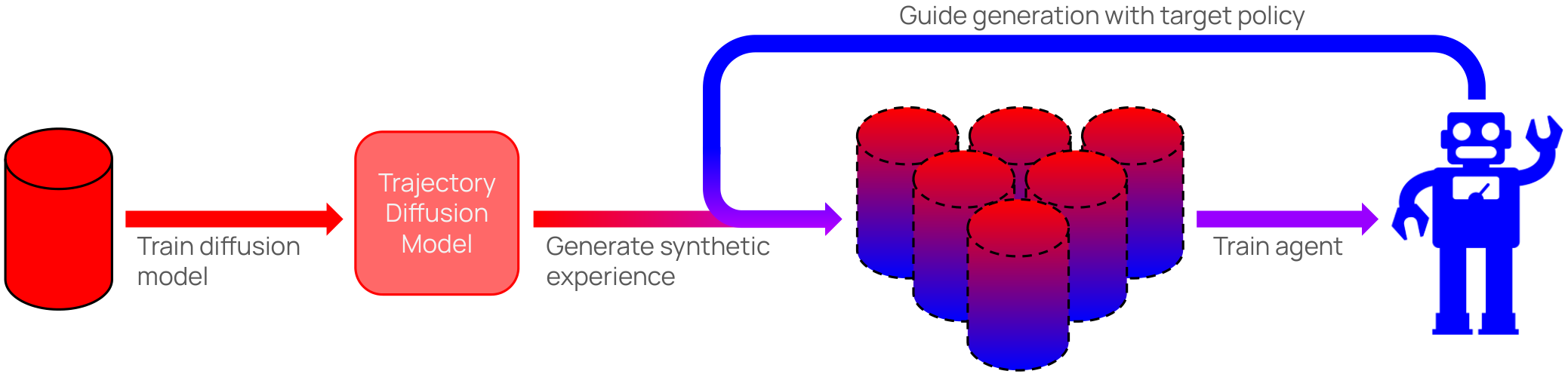
Figure 1: Offline reinforcement learning with policy-guided diffusion. Offline data from a behavior policy is first used to train a trajectory diffusion model. Synthetic experience is then generated with diffusion, guided by the target policy in order to move trajectories further on-policy. An agent is then trained for multiple steps on the synthetic dataset, before it is regenerated.

In this paper, we focus on an alternative class of methods: generating synthetic experience to both augment the offline dataset and lessen the out-of-sample issue. Prior methods in this area use a model-based approach (Yu et al., 2020; Kidambi et al., 2020; Ball et al., 2021, see Section 3.1), in which a single-step world model is learned from the offline dataset, which the target policy interacts with to generate synthetic on-policy training experience. While this allows the target policy to sample synthetic trajectories under its own action distribution, compounding model error usually forces these methods to severely truncate model rollouts to a handful of interactions. Thus, there are two options which trade off coverage and bias. The first is to roll out from the initial state, which is unbiased but lacks coverage. The second is to roll out from states randomly sampled from the data set, which increases coverage but introduces bias. Neither option fully addresses the difference in observed states between the behavior and target policy when deployed, nor the out-of-sample issue mentioned above.

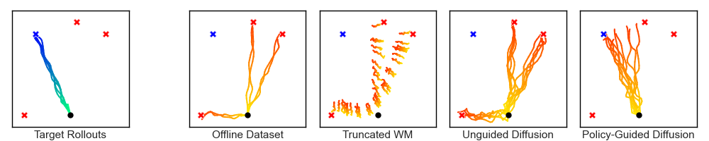
Figure 2: Trajectories from an illustrative 2D environment, in which the start location is indicated by $\bullet$ and the goals for the behavior and target policies are indicated by $\mathbf{\times}$ and $\mathbf{\times}$. Left: Rollouts from the target policy in the real environment. Right: Offline datasets gathered by the behavior policy suffer from distribution shift and limited sample size. Truncated world models (Yu et al., 2020; Kidambi et al., 2020) previously used in offline model-based reinforcement learning offer a partial solution to this problem but suffer from bias due to short rollouts. Meanwhile, unguided diffusion (Lu et al., 2023) can increase the sample size, but maintains the original distribution shift. In contrast, policy-guided diffusion samples from a regularized target distribution, generating entire trajectories with low transition error but higher likelihood under the target distribution.

Instead, we propose policy-guided diffusion (PGD, Figure 1), which avoids compounding error by modeling entire trajectories (Section 3.2) rather than single-step transitions. To achieve this, we train a diffusion model on the offline dataset, from which we can sample synthetic trajectories under the behavior policy. However, while this addresses data sparsity, these trajectories are still off-distribution from our target policy. Therefore, inspired by classifier-guided diffusion (Dhariwal & Nichol, 2021), we apply guidance from the target policy to shift the sampling distribution towards that of the target policy. At each diffusion step, our guidance term directly increases the likelihood of sampled synthetic actions under the target policy, while the diffusion model updates the entire trajectory towards those in the dataset. This yields a regularized target distribution that we name the behavior-regularized target distribution, ensuring actions do not diverge too far from the behavior policy, limiting generalization error. As a result, PGD does not suffer from compounding error, while also generating synthetic trajectories that are more representative of the target policy. We illustrate this point in Figure 2.

Our approach results in consistent improvements in offline RL performance for agents trained on policy-guided synthetic data, compared to those trained on unguided synthetic or real data. We evaluate using the standard TD3+BC (Fujimoto & Gu, 2021) and IQL (Kostrikov et al., 2021) algorithms across a variety of D4RL (Fu et al., 2020) datasets. Notably, we see a statistically significant 11.2% improvement in performance for the TD3+BC algorithm aggregated across MuJoCo (Todorov et al., 2012) locomotion tasks compared to training on the real data, with no algorithmic changes. Our results also extend to even larger improvements for the challenging Maze2d navigation environments. Furthermore, we analyze synthetic trajectories generated by PGD and show that PGD achieves lower dynamics error than PETS (Chua et al., 2018)—a prior offline model-based method—while matching the target policy likelihood of PETS. Together, our experiments illustrate the potential of PGD as an effective drop-in replacement for real data—across agents, environments, and behavior policies.

2 Background

2.1 Offline Reinforcement Learning

Formulation

We adopt the standard reinforcement learning formulation, in which an agent acts in a Markov Decision Process (MDP, Sutton & Barto, 2018). An MDP is defined as a tuple $M=\langle\mathcal{S},\mathcal{A},p_{0},T,R,H\rangle$, where $s\in\mathcal{S}$ and $a\in\mathcal{A}$ are the state and action spaces, $p_{0}(s_{0})$ is a probability distribution over the initial state, $T(s_{t+1}|s_{t},a_{t})$ is a conditional probability distribution defining the transition dynamics, $R:\mathcal{S}\times\mathcal{A}\xrightarrow{}\mathbb{R}$ is the reward function, $\gamma$ is the discount factor, and $H$ is the horizon.

In RL, we learn a policy $\pi(a|s)$ that defines a conditional probability distribution over actions for each state, inducing a distribution over trajectories $\bm{\tau}\coloneqq(s_{0},a_{1},r_{1},s_{1},\ldots,s_{H})$ given by

$$p_{\pi,M}(\bm{\tau})=p_{0}(s_{0})\prod_{t=0}^{H-1}\pi(a_{t}|s_{t})\cdot T(s_{t+1}|s_{t},a_{t})\text{,}$$ (1)

omitting the reward function throughout our work for conciseness. Our goal is to learn a policy that maximizes the expected return, defined as $\mathbb{E}_{p_{\pi,M}}[V(\bm{\tau})]$ where $V(\bm{\tau})\coloneqq\sum_{t=0}^{H}r_{t}$ is the return of a trajectory. The offline RL setting (Levine et al., 2020) extends this, preventing the agent from interacting with the environment and instead presenting it with a dataset of trajectories $\bm{\tau}\in\mathcal{D}_{\text{off}}$ gathered by some unknown behavior policy $\pi_{\text{off}}$, with which to optimize a target policy $\pi_{\text{target}}$.

Out-of-Sample Generalization

The core challenge of offline RL emerges from the distribution shift between the behavior distribution $p_{\pi_{\text{off}},M}(\bm{\tau})$ and the target distribution $p_{\pi_{\text{target}},M}(\bm{\tau})$, which are otherwise denoted $p_{\mkern 1.0mu\text{off}}(\bm{\tau})$ and $p_{\mkern 1.0mu\text{target}}(\bm{\tau})$ for conciseness. Optimization of $\pi_{\text{target}}$ on $\mathcal{D}_{\text{off}}$ can lead to catastrophic value overestimation at unobserved actions, a problem termed the out-of-sample issue (Kostrikov et al., 2021). As such, model-free offline algorithms typically regularize the policy towards the behavior distribution, either explicitly (Fujimoto & Gu, 2021; Kumar et al., 2020) or implicitly (Kostrikov et al., 2021).

Alternatively, prior work proposes learning a single-step world model $\mathcal{M}$ from $\mathcal{D}_{\text{off}}$ (Yu et al., 2020; Kidambi et al., 2020; Lu et al., 2022). By rolling out the target policy using $\mathcal{M}$, we generate trajectories $\bm{\tau}\sim p_{\mkern 1.0mu\text{target}}(\bm{\tau})$, with the aim of avoiding distribution shift. However, in practice, this technique only pushes the generalization issue into the world model. In particular, RL policies are prone to exploiting errors in the world model, which can compound over the course of an episode. When combined with typical maximizing operations used in off-policy RL, this results in value overestimation bias (Sims et al., 2024).

2.2 Diffusion Models

Definition

To generate synthetic data, we consider diffusion models (Sohl-Dickstein et al., 2015; Ho et al., 2020), a class of generative model that allows one to sample from a distribution $p(x)$ by iteratively reversing a forward noising process. Karras et al. (2022) present an ODE formulation of diffusion which, given a noise schedule $\sigma(i)$ indexed by $i$, mutates data according to

$$d\bm{x}=-\dot{\sigma}(i)\sigma(i)\nabla_{\bm{x}}\log p\left(\bm{x};\sigma(i)\right)di\text{,}$$ (2)

where $\dot{\sigma}=\frac{\mathrm{d}\sigma}{\mathrm{d}i}$ and $\nabla_{\bm{x}}\log p\left(\bm{x};\sigma(i)\right)$ is the score function (Hyvärinen & Dayan, 2005), which points towards areas of high data density. Intuitively, infinitesimal forward or backward steps of this ODE respectively nudge a sample away from or towards the data. To generate a sample, we start with pure noise at the highest noise level $\sigma_{\textrm{max}}$, and iteratively denoise in discrete timesteps under Equation 2.

Classifier Guidance

Our method is designed to augment the data-generating process towards on-policy trajectories from the target distribution $p_{\mkern 1.0mu\text{target}}(\bm{\tau})$, rather than the behavior distribution $p_{\mkern 1.0mu\text{off}}(\bm{\tau})$. To achieve this, we take inspiration from classifier guidance (Dhariwal & Nichol, 2021), which leverages a differentiable classifier to augment the score function of a pre-trained diffusion model towards a class-conditional distribution $p(\bm{x}|y)$. Concretely, this adds a classifier gradient to the score function, giving

$$\nabla_{\bm{x}}\log p_{\lambda}\left(\bm{x}|y;\sigma(i)\right)=\nabla_{\bm{x}}\log p\left(\bm{x};\sigma(i)\right)+\lambda\nabla_{\bm{x}}\log p_{\theta}\left(y|\bm{x};\sigma(i)\right)\text{,}$$ (3)

where $\nabla_{\bm{x}}\log p_{\theta}\left(y|\bm{x};\sigma(i)\right)$ is the gradient of the classifier and $\lambda$ is the guidance weight.

3 On-Policy Sampling from Offline Data

Generating synthetic agent experience is a promising approach to solving out-of-sample generalization in offline RL. By generating experience that is unseen in the dataset, the policy may be directly optimized on OOD samples, thereby moving the generalization problem from the policy to the generative model. Some prior work has suggested learning a model from the offline dataset (Lu et al., 2023), thereby sampling synthetic experience from the behavior distribution. While this improves sample coverage, the approach retains many of the original challenges of offline RL. As with the behavior policy, the synthetic trajectories may be suboptimal, meaning we still require conservative off-policy RL techniques to train the agent.

Instead, we seek to extend this approach by making our generative model sample from the target distribution. This reduces the need for conservatism and generates synthetic trajectories with increasing performance as the agent improves over training. Practically, the effectiveness of this approach depends on how we parameterize each of the terms of the trajectory distribution (Equation 1). In this section, we consider two parameterizations: autoregressive and direct.

3.1 Autoregressive Generation — Model $\bm{\mathcal{T}}$, Sample $\bm{p(s_{0})}$

The autoregressive—or model-based—approach to generating on-policy data is to use the offline dataset to train a one-step transition model $\mathcal{T}(s_{t+1}|s_{t},a_{t};\theta)$. To generate unbiased sample trajectories from the target distribution, we first sample an initial state (i.e., one that starts an episode) from the offline dataset $s_{0}\sim\mathcal{D}_{\text{off}}$. Next, we roll out our agent in the learned model by iteratively sampling actions from the target policy and approximating environment transitions with the learned dynamics model. However, compounding error from the transition model usually requires agent rollouts to be much shorter than the environment horizon—such that the agent takes $k\ll H$ steps. Consequently, any states more than $k$ steps away from any initial state cannot be generated in this manner, limiting the applicability of this approach.

As an approximation, autoregressive methods typically sample initial states from any timestep $s_{t}\sim\mathcal{D}_{\text{off}}$ in the offline dataset. Given a truncated rollout length $k$, this may be seen as approximating the sub-trajectory distribution—i.e., the trajectory from time $t$ to $t+k$—given by

$$p_{\mkern 1.0mu\text{target}}(\bm{\tau}_{t:t+k};\theta) =p_{\mkern 1.0mu\text{target}}(s_{t})\cdot p_{\mkern 1.0mu\text{target}}(\bm{\tau}_{t:t+k}|s_{t};\theta),$$ (4)

by instead modeling

$$\mathcal{F}(\bm{\tau}_{t:t+k};\theta) =p_{\mkern 1.0mu\text{off}}(s_{t})\cdot p_{\mkern 1.0mu\text{target}}(\bm{\tau}_{t:t+k}|s_{t};\theta)\text{.}$$ (5)

Here, we denote the stationary state distributions of the target and behavior policies at time $t$ by $p_{\mkern 1.0mu\text{target}}(s_{t})$ and $p_{\mkern 1.0mu\text{off}}(s_{t})$ respectively, and define the conditional sub-trajectory distribution as

$$p_{\mkern 1.0mu\text{target}}(\bm{\tau}_{t:t+k}|s_{t};\theta)\coloneqq\prod_{j=0}^{k-1} \pi_{\text{target}}(a_{t+j}|s_{t+j})\cdot\mathcal{T}(s_{t+j+1}|s_{t+j},a_{t+j};\theta)\text{.}$$ (6)

When generating trajectories from this distribution, the difference between $p_{\mkern 1.0mu\text{target}}(s_{t})$ and $p_{\mkern 1.0mu\text{off}}(s_{t})$ biases the start of rollouts towards states visited by the behavior policy. Furthermore, we still require $k$ to be small to avoid compounding error. In combination, sampling from the offline dataset “anchors” synthetic rollouts to states in the offline dataset, while truncated rollouts prevent synthetic trajectories from moving far from this anchor. Therefore, the practical application of autoregressive generation leads to a strong bias towards the behavior distribution and fails to address the out-of-sample problem.

3.2 Direct Generation — Model $\bm{p_{\mkern 1.0mu\text{{off}}}(\tau)}$

As an alternative to autoregressive generation, we can parameterize the target distribution by directly modeling the behavior distribution, as follows:

$$p_{\mkern 1.0mu\text{target}}(\bm{\tau}) =p(s_{0})\prod_{t=0}^{H-1}\pi_{\text{target}}(a_{t}|s_{t})\cdot\mathcal{T}(s_{t+1}|s_{t},a_{t})$$

$$=p(s_{0})\prod_{t=0}^{H-1}\frac{\pi_{\text{target}}(a_{t}|s_{t})}{\pi_{\text{off}}(a_{t}|s_{t})}\cdot\pi_{\text{off}}(a_{t}|s_{t})\cdot\mathcal{T}(s_{t+1}|s_{t},a_{t})$$

$$=p_{\mkern 1.0mu\text{off}}(\bm{\tau})\prod_{t=0}^{H-1}w_{a_{t},s_{t}}$$

$$\approx p_{\mkern 1.0mu\text{off}}(\bm{\tau};\theta)\prod_{t=0}^{H-1}w_{a_{t},s_{t}}=p_{\mkern 1.0mu\text{target}}(\bm{\tau};\theta)$$ (7)

where $w_{a,s}\coloneqq\frac{\pi_{\text{target}}(a|s)}{\pi_{\text{off}}(a|s)}$ denotes the importance sampling weight for $(a,s)$ (Precup, 2000). This directly parameterizes the behavior distribution $p_{\mkern 1.0mu\text{off}}(\bm{\tau};\theta)$—which may be learned by modeling entire trajectories on the offline dataset—and adjusts their likelihoods by the relative probabilities of actions $w_{a_{t},s_{t}}$ under the target and behavior policies. By jointly modeling the initial state distribution, transition function, and behavior policy, such a parameterization is not required to enforce the Markov property. As a result, it can directly generate entire trajectories, thereby avoiding the compounding model error suffered by autoregressive methods when iteratively generating transitions.

However, computing $w_{a_{t},s_{t}}$ requires access to the behavior policy $\pi_{\text{off}}(a|s)$, which is not assumed in offline RL. Prior work has explored modeling the behavior policy from the offline dataset and using this to compute importance sampling corrections. However, products of many importance weights can lead to problems with high variance (Precup et al., 2000; Levine et al., 2020).

4 Policy-Guided Diffusion

In this work, we propose a method following the direct generation approach outlined in Section 3.2, named policy-guided diffusion (PGD, LABEL:alg:generation). Following the success of diffusion models at generating trajectories (Janner et al., 2022; Lu et al., 2023), we first train a trajectory-level diffusion model on the offline dataset to model the behavior distribution. Then, inspired by classifier-guided diffusion (Section 2.2), we guide the diffusion process using the target policy to move closer to the target distribution. Specifically, during the denoising process, we compute the gradient of the action distribution for each action under the target policy, using it to augment the diffusion process towards high-probability actions. In doing so, we approximate a regularized target distribution that equally weights action likelihoods under the behavior and target policies.

In this section, we derive PGD as an approximation of the behavior-regularized target distribution (Section 4.1), then describe practical details for controlling and stabilizing policy guidance (Section 4.2). We provide a summary of PGD against alternative sources of training data in Table 1.

4.1 Behavior-Regularized Target Distribution

Policy Guidance Derivation

To sample a trajectory via diffusion, we require a noise-conditioned score function $\nabla_{\bm{\hat{\tau}}}\log p(\bm{\hat{\tau}};\sigma)$ for a noised trajectory $\bm{\hat{\tau}}\coloneqq(\hat{s}_{0},\hat{a}_{1},\hat{r}_{1},\hat{s}_{1},\ldots,\hat{s}_{H})$ under a distribution $p(\bm{\tau})$ at a noise level $\sigma$. Given an offline dataset $\mathcal{D}_{\text{off}}$, it is straightforward to learn this function under the behavior distribution, $\nabla_{\bm{\hat{\tau}}}\log p_{\mkern 1.0mu\text{off}}(\bm{\hat{\tau}};\sigma)$, by training a denoiser model to reconstruct noised trajectories from $\mathcal{D}_{\text{off}}$. However, there is no apparent method to directly model the noise-conditioned score function $\nabla_{\bm{\hat{\tau}}}\log p_{\mkern 1.0mu\text{target}}(\bm{\hat{\tau}};\sigma)$ for the target distribution (see Appendix B for further discussion), meaning we require an approximation.

To achieve this, we consider the score function of a noise-free trajectory $\bm{\tau}$ under the target distribution, based on the formulation from Equation 7,

$$\nabla_{\bm{\tau}}\log p_{\mkern 1.0mu\text{target}}(\bm{\tau})=\nabla_{\bm{\tau}}\log p_{\mkern 1.0mu\text{off}}(\bm{\tau})+\sum_{t=0}^{H-1}\left(\nabla_{\bm{\tau}}\log\pi_{\text{target}}\left(a_{t}|s_{t}\right)-\nabla_{\bm{\tau}}\log\pi_{\text{off}}\left(a_{t}|s_{t}\right)\right)\text{.}$$ (8)

In the limit of noise $\sigma\to 0$, the noise-conditioned score function $\nabla_{\bm{\hat{\tau}}}\log p_{\mkern 1.0mu\text{target}}(\bm{\hat{\tau}};\sigma)$ clearly approaches $\nabla_{\bm{\tau}}\log p_{\mkern 1.0mu\text{target}}(\bm{\tau})$. Therefore, we may approximate this function by

$$\nabla_{\bm{\hat{\tau}}}\log p_{\mkern 1.0mu\text{target}}(\bm{\hat{\tau}};\sigma)\approx\nabla_{\bm{\hat{\tau}}}\log p_{\mkern 1.0mu\text{off}}(\bm{\hat{\tau}};\sigma)+\sum_{t=0}^{H-1}\left(\nabla_{\bm{\hat{\tau}}}\log\pi_{\text{target}}\left(\hat{a}_{t}|\hat{s}_{t}\right)-\nabla_{\bm{\hat{\tau}}}\log\pi_{\text{off}}\left(\hat{a}_{t}|\hat{s}_{t}\right)\right)\text{,}$$ (9)

for $\sigma\approx 0$. Whilst iteratively denoising under this function (Section 2.2) does not model $p_{\mkern 1.0mu\text{target}}(\bm{\tau})$ exactly, the score function approaches $\nabla_{\bm{\hat{\tau}}}\log p_{\mkern 1.0mu\text{target}}(\bm{\hat{\tau}};\sigma)$ towards the end of the denoising process, which we believe provides an effective approximation.

Excluding Behavior Policy Guidance

As discussed, we may directly model the first term of Equation 9 by training a denoiser model. Furthermore, we may directly compute target policy guidance $\nabla_{\bm{\hat{\tau}}}\log\pi_{\text{target}}\left(\hat{a}_{t}|\hat{s}_{t}\right)$—the second term of this approximation—as we assume access to a (differentiable) target policy in the offline RL setting. However, we generally do not have access to the behavior policy, preventing us from computing $\nabla_{\bm{\hat{\tau}}}\log\pi_{\text{off}}\left(\hat{a}_{t}|\hat{s}_{t}\right)$. Due to this, we exclude behavior policy guidance from our approximation, resulting in the score function $\nabla_{\bm{\hat{\tau}}}\log p_{\mkern 1.0mu\text{off}}(\bm{\hat{\tau}};\sigma)+\sum_{t=0}^{H-1}\nabla_{\bm{\hat{\tau}}}\log\pi_{\text{target}}\left(\hat{a}_{t}|\hat{s}_{t}\right)$. As $\sigma\to 0$, this approaches the score function for a proxy distribution of the form

$$\mathcal{F}(\bm{\tau};\pi_{\text{target}}) \propto p_{\mkern 1.0mu\text{off}}(\bm{\tau})\prod_{t=0}^{H-1}\pi_{\text{target}}(a_{t}|s_{t})$$

$$=p_{\mkern 1.0mu\text{off}}(\bm{\tau})\cdot q_{\mkern 1.0mu\text{target}}(\bm{\tau})=p_{\mkern 1.0mu\text{target}}(\bm{\tau})\cdot q_{\mkern 1.0mu\text{off}}(\bm{\tau})\text{,}$$ (10)

where $q_{\mkern 1.0mu\text{target}}(\bm{\tau})\coloneqq\prod_{t=0}^{H-1}\pi_{\text{target}}(a_{t}|s_{t})$ denotes the product of action probabilities under the target policy and $q_{\mkern 1.0mu\text{off}}(\bm{\tau})$ denotes the same quantity under the behavior policy. Therefore, we hypothesize that excluding behavior policy guidance is an effective form of regularization, as it biases trajectories towards the support of the offline data, thereby limiting model error and the out-of-sample problem. We refer to $\mathcal{F}(\bm{\tau};\pi_{\text{target}})$ as the behavior-regularized target distribution due to it balancing action likelihoods under the behavior and target policies, and provide further discussion in Appendix C. Finally, as a promising avenue for future work, we note that the behavior policy may be modeled by applying behavior cloning to $\mathcal{D}_{\text{off}}$, allowing for the inclusion of behavior policy guidance in the offline RL setting.

Excluding State Guidance

Target policy guidance $\nabla_{\bm{\hat{\tau}}}\log\pi_{\text{target}}\left(\hat{a}_{t}|\hat{s}_{t}\right)$ has non-zero gradients for the state and action at timestep $t$. In practice, the action component $\nabla_{\hat{a}_{t}}\log\pi_{\text{target}}\left(\hat{a}_{t}|\hat{s}_{t}\right)$ typically has an efficient, closed-form solution, with $\pi_{\text{target}}\left(\hat{a}_{t}|\hat{s}_{t}\right)$ commonly being Gaussian for continuous action spaces. In contrast, for neural network policies, the state component $\nabla_{\hat{s}_{t}}\log\pi_{\text{target}}\left(\hat{a}_{t}|\hat{s}_{t}\right)$ requires backpropagating gradients through the policy network, which is both expensive to compute and can lead to high variance on noisy, out-of-distribution states. Due to this, we apply policy guidance to only the noised action, yielding our policy-guided score function

$$s_{\mkern 1.0mu\text{PGD}}(\bm{\hat{\tau}};\sigma)=\underbrace{\nabla_{\bm{\hat{\tau}}}\log p_{\mkern 1.0mu\text{off}}(\bm{\hat{\tau}};\sigma)}_{\mathclap{\text{Behavior score function}}}+\underbrace{\nabla_{\bm{\hat{a}}}\log q_{\mkern 1.0mu\text{target}}(\bm{\hat{\tau}})}_{\mathclap{\text{Target policy guidance}}}\text{,}$$ (11)

where (abusing notation) $\nabla_{\bm{\hat{a}}}$ denotes the gradient $\nabla_{\bm{\hat{\tau}}}$ of $\bm{\hat{\tau}}$, with non-action components set to 0.

4.2 Improving Policy Guidance

Controlling Guidance Strength

A standard technique from classifier-guided diffusion is the use of guidance coefficients (Dhariwal & Nichol, 2021). These augment the guided score function by introducing a controllable coefficient on the guidance term. Applied to the PGD score function (Equation 11), this has the form

$$s_{\mkern 1.0mu\text{PGD}}(\bm{\hat{\tau}};\sigma,\lambda)=\nabla_{\bm{\hat{\tau}}}\log p_{\mkern 1.0mu\text{off}}(\bm{\hat{\tau}};\sigma)+\lambda\nabla_{\bm{\hat{a}}}\log q_{\mkern 1.0mu\text{target}}(\bm{\hat{\tau}})\text{,}$$ (12)

where $\lambda$ denotes the guidance coefficient. As $\sigma\to 0$, this transforms the sampling distribution to

$$\mathcal{F}(\bm{\tau}|\pi_{\text{target}};\lambda)\propto p_{\mkern 1.0mu\text{off}}(\bm{\tau})\cdot q_{\mkern 1.0mu\text{target}}(\bm{\tau})^{\lambda}\text{.}$$ (13)

Intuitively, $\lambda$ interpolates the actions in the sampling distribution between the behavior and target distributions. By tuning $\lambda$, we can therefore control the strength of guidance towards the target policy, avoiding high dynamics error when the target policy is far from the behavior policy. We visualize this effect in Figure 3 and analyze its impact on target policy likelihood in Figure 5.

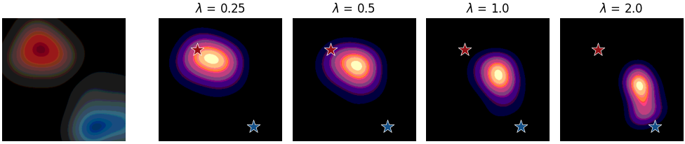
Figure 3: Left: Trajectory probability distribution for an example behavior distribution $p_{\mkern 1.0mu\text{off}}(\bm{\tau})$ and target policy likelihood $q_{\mkern 1.0mu\text{target}}(\bm{\tau})$. Right: Corresponding PGD sampling distribution (Equation 13) computed over a range of policy-guidance coefficients $\lambda$. By increasing $\lambda$, we transform from the sampling distribution towards the regions of high target policy likelihood, making PGD an effective mechanism for controlling the level of regularization towards the behavior distribution.

Following Ma et al. (2023), we also apply a cosine guidance schedule to the guidance coefficient,

$$\lambda_{n}=\lambda\cdot(\sigma_{n}+\beta\sigma_{N}\cdot\sin(\pi\cdot n/N))\text{,}$$ (14)

where $\beta$ is the cosine weight, which is set to 0.3 in all experiments. By decreasing the strength of guidance in later steps, we find that this schedule stabilizes guidance and reduces dynamics error.

Stabilizing Guided Diffusion

When under distribution shift, RL policies are known to suffer from poor generalization to unseen states (Kirk et al., 2023). This makes policy guidance challenging, since the policy must operate on noised states, and compute action gradients from noised actions. Similar issues have been studied in classifier-guided diffusion (Ma et al., 2023), where the classifier gradient can be unstable when exposed to out-of-distribution inputs. Bansal et al. (2023) alleviate this issue by applying guidance to the denoised sample estimated by the denoiser model, rather than the original noised sample, in addition to normalizing the guidance gradient to a unit vector. By applying these techniques to policy guidance, we lessen the need for the target policy to generalize to noisy states, which we find decreases dynamics error.

Table 1: Overview of training experience sources in offline RL—for each, we consider the sampling distribution, expected error in transition dynamics, likelihood of actions under the target policy, and state space coverage beyond the behavior distribution. Policy-guided diffusion provides an effective trade-off between each error, likelihood, and coverage.

Data source	Distribution	Error ($\bm{\downarrow}$)	Likelihood ($\bm{\uparrow}$)	Coverage ($\bm{\uparrow}$)
Offline dataset	$p_{\mkern 1.0mu\text{off}}(\bm{\tau})$	—	Low	Low
Episodic world model	$p_{\mkern 1.0mu\text{target}}(\bm{\tau})$	High	—	High
Truncated world model	Equation 5	Low	—	Low
Unguided diffusion	$p_{\mkern 1.0mu\text{off}}(\bm{\tau})$	Low	Low	High
Policy-guided diffusion	Equation 10	Low	High	High

5 Results

Through our experiments, we first demonstrate that agents trained with synthetic experience from PGD outperform those trained on unguided synthetic data or directly on the offline dataset (Section 5.2). We show that this effect is consistent across agents (TD3+BC and IQL), environments (HalfCheetah, Walker2d, Hopper, and Maze), behavior policies (random, mixed, and medium), and modes of data generation (continuous and periodic). Following this, we demonstrate that tuning the guidance coefficient enables PGD to sample trajectories with high action likelihood across a range of target policies. Finally, we verify that PGD retains low dynamics error despite sampling high-likelihood actions from the policy (Section 5.3).

5.1 Experimental Setup

We evaluate PGD on the MuJoCo and Maze2d continuous control datasets from D4RL (Fu et al., 2020; Todorov et al., 2012). For MuJoCo, we consider the HalfCheetah, Walker2d, and Hopper environments with random (randomly initialized behavior policy), medium (suboptimal behavior policy), and medium-replay (or “mixed”, the replay buffer from medium policy training) datasets. For Maze2d we consider the original (sparse reward) instances of the umaze, medium and large layouts. We train 4 trajectory diffusion models on each dataset, for which we detail hyperparameters in Appendix A. In Section 5.3, we conduct analysis of PGD against MOPO-style PETS (Chua et al., 2018) models, an autoregressive world model composed of an ensemble of probabilistic models, for which we use model weights from OfflineRL-Kit (Sun, 2023).

To demonstrate synthetic experience from PGD as a drop-in substitute for the real dataset, we transfer the original hyperparameters for IQL (Kostrikov et al., 2021) and TD3+BC (Fujimoto & Gu, 2021)—as tuned on the real datasets—without any further tuning. Policy guidance requires a stochastic target policy, in order to compute the gradient of the action distribution. Since TD3+BC trains a deterministic policy, we perform guidance by modeling the action distribution as a unit Gaussian centered on the deterministic action. We implement all agents and diffusion models from scratch in Jax (Bradbury et al., 2018), which may be found at https://github.com/EmptyJackson/policy-guided-diffusion.

5.2 Offline Reinforcement Learning

For each D4RL dataset, we train two popular model-free offline algorithms, TD3+BC (Fujimoto & Gu, 2021) and IQL (Kostrikov et al., 2021) on synthetic experience generated by trajectory diffusion models with and without policy guidance, as well as on the real dataset. We first consider periodic generation of synthetic data, in which the synthetic dataset is regenerated after extended periods of agent training, such that the agent is near convergence on the synthetic dataset at the point it is regenerated with the current policy. Each epoch, we generate a dataset of $2^{14}$ synthetic trajectories of length 16. Following the notation of LABEL:alg:training, we set the number of epochs to $N_{\text{epochs}}=4$ with $N_{\text{policy}}=$250,000$$ train steps per epoch, meaning the agent is trained to close to convergence before the dataset is regenerated. This can be viewed as solving a sequence of offline RL tasks with synthetic datasets, in which the behavior policy is the target policy from the previous generation.

Using periodic generation, performance improves significantly across benchmarks for both IQL and TD3+BC (Table 2). In MuJoCo, the most consistent improvement is on mixed datasets, with 4 out of 6 experiments achieving significant performance improvement. This is to be expected, as these datasets contain experience from a mixture of behavior policy levels. In this case, the diffusion model is likely to be able to represent a wide variety of policies, and on-policy guidance would naturally produce higher return trajectories as the target policy improves.

Table 2: Final return of IQL and TD3+BC agents trained on real, unguided ($\lambda=0$) synthetic and policy-guided ($\lambda=1$) synthetic data—mean and standard error over 4 seeds (diffusion models and agents) is presented, with significant improvements ($p<0.05$) shaded.

		IQL												TD3+BC
			Dataset			Unguided			Guided					Dataset			Unguided			Guided
Random	HalfCheetah		$\displaystyle 9.1$	$\pm$	$2.2$	$2.6$	$\pm$	$0.1$	$\displaystyle 6.5$	$\pm$	$1.7$			$11.2$	$\pm$	$0.8$	$11.0$	$\pm$	$0.4$	$\displaystyle 21.1$	$\pm$	$0.9$
	Walker2d		$4.3$	$\pm$	$0.5$	$2.7$	$\pm$	$0.7$	$\displaystyle 5.3$	$\pm$	$0.3$			$0.5$	$\pm$	$0.3$	$1.1$	$\pm$	$1.2$	$-0.3$	$\pm$	$0.1$
	Hopper		$\displaystyle 7.4$	$\pm$	$0.4$	$5.2$	$\pm$	$0.9$	$4.9$	$\pm$	$1.0$			$7.4$	$\pm$	$0.6$	$4.2$	$\pm$	$1.4$	$5.5$	$\pm$	$2.1$
Mixed	HalfCheetah		$\displaystyle 44.2$	$\pm$	$0.2$	$43.6$	$\pm$	$0.2$	$43.6$	$\pm$	$0.2$			$44.7$	$\pm$	$0.1$	$43.1$	$\pm$	$0.2$	$\displaystyle 46.1$	$\pm$	$0.3$
	Walker2d		$81.3$	$\pm$	$2.0$	$\displaystyle 85.2$	$\pm$	$0.3$	$\displaystyle 84.9$	$\pm$	$1.4$			$82.7$	$\pm$	$1.3$	$70.7$	$\pm$	$10.1$	$84.0$	$\pm$	$1.0$
	Hopper		$82.9$	$\pm$	$3.5$	$\displaystyle 97.4$	$\pm$	$2.7$	$\displaystyle 100.5$	$\pm$	$0.5$			$58.6$	$\pm$	$11.2$	$52.1$	$\pm$	$1.8$	$\displaystyle 91.9$	$\pm$	$4.3$
Medium	HalfCheetah		$\displaystyle 48.4$	$\pm$	$0.1$	$45.4$	$\pm$	$0.1$	$45.1$	$\pm$	$0.1$			$\displaystyle 48.6$	$\pm$	$0.1$	$45.3$	$\pm$	$0.2$	$47.6$	$\pm$	$0.3$
	Walker2d		$81.7$	$\pm$	$1.4$	$82.1$	$\pm$	$0.9$	$77.8$	$\pm$	$3.6$			$84.8$	$\pm$	$0.1$	$85.2$	$\pm$	$0.2$	$\displaystyle 86.3$	$\pm$	$0.3$
	Hopper		$63.6$	$\pm$	$0.8$	$59.7$	$\pm$	$2.0$	$62.8$	$\pm$	$1.2$			$\displaystyle 62.4$	$\pm$	$0.9$	$57.4$	$\pm$	$0.4$	$\displaystyle 63.1$	$\pm$	$0.6$
	Total		$46.9$	$\pm$	$0.4$	$47.0$	$\pm$	$0.4$	$\displaystyle 47.9$	$\pm$	$0.3$			$44.5$	$\pm$	$1.1$	$41.1$	$\pm$	$1.1$	$\displaystyle 49.5$	$\pm$	$0.9$
Maze2d	UMaze		$42.6$	$\pm$	$0.4$	$42.9$	$\pm$	$1.8$	$43.8$	$\pm$	$3.5$			$50.0$	$\pm$	$2.4$	$33.8$	$\pm$	$3.0$	$\displaystyle 76.2$	$\pm$	$17.4$
	Medium		$38.5$	$\pm$	$1.9$	$33.4$	$\pm$	$3.2$	$\displaystyle 60.0$	$\pm$	$13.9$			$32.1$	$\pm$	$6.8$	$24.0$	$\pm$	$4.0$	$\displaystyle 89.6$	$\pm$	$19.9$
	Large		$\displaystyle 50.9$	$\pm$	$5.8$	$23.4$	$\pm$	$8.0$	$\displaystyle 45.3$	$\pm$	$14.8$			$137.2$	$\pm$	$20.2$	$93.3$	$\pm$	$31.0$	$131.1$	$\pm$	$37.5$
	Total		$\displaystyle 44.0$	$\pm$	$2.2$	$33.2$	$\pm$	$1.8$	$\displaystyle 49.7$	$\pm$	$9.5$			$73.1$	$\pm$	$6.7$	$50.4$	$\pm$	$11.1$	$\displaystyle 99.0$	$\pm$	$14.5$

In order to demonstrate the flexibility of PGD, we also evaluate PGD in a continuous generation setting, using a data generation rate closer to that of traditional model-based methods. For this, we set $N_{\text{epochs}}=$100$$ and $N_{\text{policy}}=$10,000$$, then lower the sample size to match the overall number of synthetic trajectories generated by periodic generation across training. Due to the decrease in sample size, we maintain each generated dataset across epochs in a replay buffer, with each dataset being removed after 10 epochs.

We see similar improvements in performance against real and unguided synthetic data under this approach, with PGD outperforming real data on 2 out of 3 environments and datasets (Figure 4). Periodic generation outperforms continuous generation across environments and behavior policies, which we attribute to training stability, especially when performing guidance early in training. Regardless, both approaches consistently outperform training on real and unguided synthetic data, demonstrating the potential of PGD as a drop-in extension to replay and model-based RL methods.

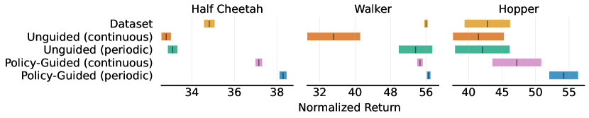
(a) Environments

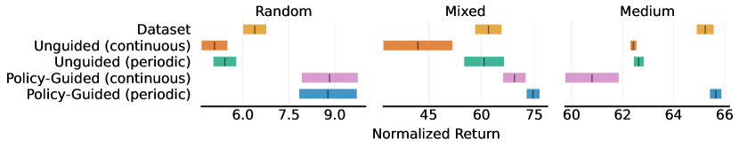
(b) Behavior policies

Figure 4: Aggregate MuJoCo performance after training on unguided or policy-guided synthetic data under continuous and periodic dataset generation, as well as on the real dataset. For each setting, mean return over TD3+BC and IQL agents is marked, with standard error over 4 seeds (diffusion models and agents) highlighted.

5.3 Synthetic Trajectory Analysis

We now analyze the quality of trajectories produced by PGD against those from unguided diffusion and autoregressive world model (PETS) rollouts. In principle, we seek to evaluate the divergence of these sampling distributions from the true target distribution. However, this is not tractable to compute directly, so we instead investigate two proxy objectives:

1. Trajectory Likelihood: mean log-likelihood of actions under the target policy; and

2. Dynamics Error: mean squared error between states in the synthetic trajectory and real environment, when rolled out with the same initial state and action sequence.

In our experiments, we consider trajectory diffusion and MOPO-style PETS (Chua et al., 2018) models trained on representative datasets from the D4RL (Fu et al., 2020) benchmark that were featured in the previous section. Specifically, we consider the models trained on halfcheetah-medium, before sampling trajectories with IQL target policies trained on the halfcheetah-random, -medium, and -expert. This enables us to test the robustness of these models to target policies far from the behavior policy, both in performance and policy entropy.

Policy Guidance Increases Trajectory Likelihood

In Figure 5, we present the trajectory likelihood of synthetic trajectories over varying degrees of guidance. Unsurprisingly, unguided diffusion generates low probability trajectories for all target policies, due to it directly modeling the behavior distribution. However, as we increase the guidance coefficient $\lambda$, trajectory likelihood increases monotonically under each target policy. Furthermore, this effect is robust across target policies, giving the ability to sample high-probability trajectories with OOD target policies. The value of $\lambda$ required to achieve the same action likelihood as direct action sampling (PETS) varies with the target policy. Since this threshold increases with target policy performance, we hypothesize that it increases with target policy entropy. Based on this, a promising avenue for future work is automatically tuning $\lambda$ for hyperparameter-free guidance.

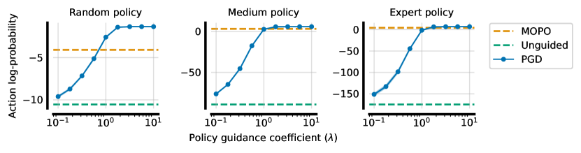
Figure 5: Action probability of synthetic trajectories generated by diffusion and PETS models trained on halfcheetah-medium. Target policies are trained on halfcheetah-random, halfcheetah-medium, and halfcheetah-expert datasets, demonstrating robustness to OOD actions. Standard error over 4 diffusion model seeds is shaded (but negligible), with mean computed over 2048 synthetic trajectories.

Policy Guided Diffusion Achieves Lower Error Than Autoregressive Models

In Figure 6, we present the dynamics error of synthetic trajectories over 16 rollout steps. For a fair comparison, we fix the guidance coefficient of PGD to $\lambda=1.0$, since this was sufficient to match the trajectory likelihood of PETS (Figure 5). Over all target policies, PGD achieves significantly lower error than PETS. Furthermore, PGD has similar levels of error across target policies, while PETS suffers from significantly higher error on OOD (random and expert) target policies. This highlights the robustness of PGD to target policy, a critical feature for generating high-likelihood training data throughout tabula rasa policy training.

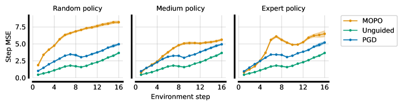
Figure 6: Dynamics mean squared error of synthetic trajectories generated by diffusion and PETS models trained on halfcheetah-medium. Standard error over 4 diffusion model seeds and 3 PETS seeds (via OfflineRL-Kit) is shaded, with each generating 2048 synthetic trajectories for analysis.

6 Related Work

Model-based Offline Reinforcement Learning

Model-based methods in offline RL (Yu et al., 2020; Kidambi et al., 2020; Rigter et al., 2022; Lu et al., 2022) are designed to augment the offline buffer with additional on-policy samples in order to mitigate distribution shift. This is typically done by rolling out a policy in a learned world model (Janner et al., 2019) and applying a suitable pessimism term in order to account for dynamics model errors. While these methods share the same overall motivation as our paper, the empirical realization is quite different. In particular, forward dynamics models are liable to compounding errors over long horizons, resulting in model exploitation, whereas our trajectories are generated in a single step.

Model-free Offline Reinforcement Learning

Model-free methods in offline RL typically tackle the out-of-sample issue by applying conservatism to the value function or by constraining the policy to remain close to the data. For example, CQL (Kumar et al., 2020) and EDAC (An et al., 2021) both aim to minimize the values of out-of-distribution actions. Meanwhile, BCQ (Fujimoto et al., 2019) ensures that actions used in value targets are in-distribution with the behavioral policy using constrained optimization. We take the opposite approach in this paper: by enabling our diffusion model to generate on-policy samples without diverging from the behavior distribution, we reduce the need for conservatism.

Diffusion in Reinforcement Learning

Diffusion models are a flexible method for data augmentation in reinforcement learning. SynthER (Lu et al., 2023) uses unguided diffusion models to upsample offline or online RL datasets, which are then used by model-free off-policy algorithms. While this improves performance, SynthER uses unguided diffusion to model the behavior distribution, resulting in the same issue of distributional shift. Similarly, MTDiff (He et al., 2023) considers unguided data generation in multitask settings.

Diffusion models have also been used to train world models. Zhang et al. (2023) train a world model for sensor observations by first tokenizing using VQ-VAE and then predicting future observations via discrete diffusion. Alonso et al. (2023) also train a world model using diffusion and demonstrate it can more accurately predict future observations. However, neither of these approaches model the whole trajectory, thereby suffering from compounding error, nor do they apply policy guidance. Parallel to this work, Rigter et al. (2023) use guidance from a policy to augment a diffusion world model for online RL. By contrast, we focus on the offline RL setting, provide a theoretical derivation and motivation for the trajectory distribution modeled by policy guidance, and demonstrate improvements in downstream policy performance.

Diffusion models are also used elsewhere in reinforcement learning. For example, Diffuser (Janner et al., 2022) and Decision Diffuser (Ajay et al., 2023) use trajectory diffusion models for planning and to bias planned trajectories towards high return. By contrast, we use on-policy guidance and train on the generated data. Diffusion models have also been used as an expressive policy class (Wang et al., 2023) for $Q$-learning, showing improvement over MLPs.

7 Conclusion

We presented policy-guided diffusion, a method for controllable generation of synthetic trajectories in offline RL. We provided a theoretical analysis of existing approaches to synthetic experience generation, identifying the advantages of direct trajectory generation compared to autoregressive methods. Motivated by this, we proposed PGD under the direct approach, deriving the regularized target distribution modeled by policy guidance.

Evaluating against PETS deep ensembles, a state-of-the-art autoregressive approach, we found that PGD can generate synthetic experience at the same target policy likelihood with significantly lower dynamics error. Furthermore, we found consistent improvements in downstream agent performance over a range of environments and behavior policies when trained on policy-guided synthetic data, against real and unguided synthetic experience.

By addressing the out-of-sample issue through synthetic data, we hope that this work enables the development of less conservative algorithms for offline RL. There are a range of promising avenues for future work, including automatically tuning the guidance coefficient for hyperparameter-free guidance, leveraging on-policy RL techniques with policy-guided data, and extending this approach to large-scale video generation models.

Acknowledgments

We thank Mattie Fellows and Sebastian Towers for their insights regarding our method’s theoretical underpinning, as well as Alex Goldie and the NeurIPS 2023 Robot Learning Workshop reviewers for their helpful feedback. Matthew Jackson is funded by the EPSRC Centre for Doctoral Training in Autonomous Intelligent Machines and Systems, and Amazon Web Services.

Appendix

Appendix A Hyperparameters

We open-source our implementation at https://github.com/EmptyJackson/policy-guided-diffusion.

A.1 Diffusion Model

For the diffusion model, we used a U-Net architecture (Ronneberger et al., 2015) with hyperparameters outlined in Table 3. We transformed the trajectory by stacking the observation, action, reward, and done flags for each transition, before performing 1D convolution across the sequence of transitions.

Table 3: U-Net hyperparameters

Hyperparameter	Value
Trajectory length	16
Kernel size	3
Features	1024
U-Net blocks	3
Batch size	16
Dataset epochs	250
Optimizer	Adam
Learning rate	$2\times 10^{-3}$
LR schedule	Cosine decay

A.2 Diffusion Sampling

We use EDM (Karras et al., 2022) for diffusion sampling, retaining many of the default hyperparameters from Lu et al. (2023) (Table 4). We tuned the number of diffusion timesteps, finding diminishing improvement in dynamics error beyond 256 timesteps.

Table 4: EDM hyperparameters

Hyperparameter	Value
Diffusion timesteps	256
$\text{S}_{\text{churn}}$	80
$\text{S}_{\text{noise}}$	$1.003$
$\text{S}_{\text{tmax}}$	50
$\text{S}_{\text{tmin}}$	$0.05$
$\sigma_{\text{max}}$	80
$\sigma_{\text{min}}$	$0.002$

Appendix B Noised Target Distribution

To model the target distribution with diffusion, we require the noise-conditioned score function $\nabla_{\bm{\hat{\tau}}}\log p_{\mkern 1.0mu\text{target}}(\bm{\hat{\tau}};\sigma)$ for the target distribution. However, since we do not have access to samples from $p_{\text{target}}(\bm{\hat{\tau}};\sigma)$, one might wish to apply a factorization of the target distribution, such as

$$p_{\mkern 1.0mu\text{target}}(\bm{\tau}) =p_{\mkern 1.0mu\text{off}}(\bm{\tau})\prod_{t=0}^{H-1}\frac{\pi_{\text{target}}(a|s)}{\pi_{\text{off}}(a|s)}\text{,}$$ (15)

before modeling its terms separately. However, by applying independent Gaussian noise to each of the elements in $\bm{\hat{\tau}}$, we lose conditional independence between contiguous states and actions—i.e., $p_{\mkern 1.0mu\text{target}}(\hat{a}_{t}|\bm{\hat{\tau}}\!\setminus\!\hat{a}_{t};\sigma)\neq p_{\mkern 1.0mu\text{target}}(\hat{a}_{t}|\hat{s}_{t};\sigma)$—preventing us from applying an equivalent factorization. Due to this, we must approximate $\nabla_{\bm{\hat{\tau}}}\log p_{\mkern 1.0mu\text{target}}(\bm{\hat{\tau}};\sigma)$ directly, as we propose in Section 4.1.

Appendix C Behavior-Regularized Target Distribution

Intuitively, the behavior-regularized target distribution transforms the target distribution by increasing the likelihood of actions under the behavior policy. As is typical in offline RL (Kumar et al., 2020; Fujimoto & Gu, 2021; Fujimoto et al., 2019), regularizing the policy towards the behavior distribution is required in order to avoid out-of-sample states and consequently minimize value overestimation. Rather than regularizing the policy, PGD shifts this regularization to the data generation process, which helps our guided samples remain in-distribution with respect to the diffusion model, and thus less susceptible to model error.

Moreover, we note that this type of regularization is not immediately available for prior autoregressive world models, and thus they typically penalize reward by dynamics error (Yu et al., 2020; Kidambi et al., 2020; Lu et al., 2022) in an ad-hoc fashion in order to avoid model exploitation. In contrast, PGD presents a natural mechanism for behavioral regularization during data generation, making offline policy optimization without regularization a promising path for future work.

Appendix D Agent Training with Policy-Guided Diffusion

In LABEL:alg:training, we present pseudocode for training an agent with synthetic experience generated by PGD. PGD is agnostic to the underlying offline RL algorithm used to train the target policy, making it a drop-in extension to any model-free method.

References

- Ajay et al. (2023) Anurag Ajay, Yilun Du, Abhi Gupta, Joshua B. Tenenbaum, Tommi S. Jaakkola, and Pulkit Agrawal. Is conditional generative modeling all you need for decision making? In The Eleventh International Conference on Learning Representations, 2023. URL https://openreview.net/forum?id=sP1fo2K9DFG.
- Alonso et al. (2023) Eloi Alonso, Adam Jelley, Anssi Kanervisto, and Tim Pearce. Diffusion world models. 2023.
- An et al. (2021) Gaon An, Seungyong Moon, Jang-Hyun Kim, and Hyun Oh Song. Uncertainty-based offline reinforcement learning with diversified q-ensemble. Advances in neural information processing systems, 34:7436–7447, 2021.
- Ball et al. (2021) Philip J Ball, Cong Lu, Jack Parker-Holder, and Stephen Roberts. Augmented world models facilitate zero-shot dynamics generalization from a single offline environment. In Marina Meila and Tong Zhang (eds.), Proceedings of the 38th International Conference on Machine Learning, volume 139 of Proceedings of Machine Learning Research, pp. 619–629. PMLR, 18–24 Jul 2021.
- Bansal et al. (2023) Arpit Bansal, Hong-Min Chu, Avi Schwarzschild, Soumyadip Sengupta, Micah Goldblum, Jonas Geiping, and Tom Goldstein. Universal guidance for diffusion models. In Proceedings of the IEEE/CVF Conference on Computer Vision and Pattern Recognition, pp. 843–852, 2023.
- Bradbury et al. (2018) James Bradbury, Roy Frostig, Peter Hawkins, Matthew James Johnson, Chris Leary, Dougal Maclaurin, George Necula, Adam Paszke, Jake VanderPlas, Skye Wanderman-Milne, and Qiao Zhang. JAX: composable transformations of Python+NumPy programs, 2018. URL http://github.com/google/jax.
- Chua et al. (2018) Kurtland Chua, Roberto Calandra, Rowan McAllister, and Sergey Levine. Deep reinforcement learning in a handful of trials using probabilistic dynamics models, 2018.
- Dhariwal & Nichol (2021) Prafulla Dhariwal and Alexander Nichol. Diffusion models beat gans on image synthesis. Advances in neural information processing systems, 34:8780–8794, 2021.
- Fu et al. (2020) Justin Fu, Aviral Kumar, Ofir Nachum, George Tucker, and Sergey Levine. D4rl: Datasets for deep data-driven reinforcement learning. arXiv preprint arXiv:2004.07219, 2020.
- Fujimoto & Gu (2021) Scott Fujimoto and Shixiang Shane Gu. A minimalist approach to offline reinforcement learning. In Thirty-Fifth Conference on Neural Information Processing Systems, 2021.
- Fujimoto et al. (2019) Scott Fujimoto, David Meger, and Doina Precup. Off-policy deep reinforcement learning without exploration. In Kamalika Chaudhuri and Ruslan Salakhutdinov (eds.), Proceedings of the 36th International Conference on Machine Learning, volume 97 of Proceedings of Machine Learning Research, pp. 2052–2062. PMLR, 09–15 Jun 2019. URL https://proceedings.mlr.press/v97/fujimoto19a.html.
- He et al. (2023) Haoran He, Chenjia Bai, Kang Xu, Zhuoran Yang, Weinan Zhang, Dong Wang, Bin Zhao, and Xuelong Li. Diffusion model is an effective planner and data synthesizer for multi-task reinforcement learning. arXiv preprint arXiv:2305.18459, 2023.
- Ho et al. (2020) Jonathan Ho, Ajay Jain, and Pieter Abbeel. Denoising diffusion probabilistic models. In H. Larochelle, M. Ranzato, R. Hadsell, M.F. Balcan, and H. Lin (eds.), Advances in Neural Information Processing Systems, volume 33, pp. 6840–6851. Curran Associates, Inc., 2020. URL https://proceedings.neurips.cc/paper/2020/file/4c5bcfec8584af0d967f1ab10179ca4b-Paper.pdf.
- Hyvärinen & Dayan (2005) Aapo Hyvärinen and Peter Dayan. Estimation of non-normalized statistical models by score matching. Journal of Machine Learning Research, 6(4), 2005.
- Janner et al. (2019) Michael Janner, Justin Fu, Marvin Zhang, and Sergey Levine. When to trust your model: Model-based policy optimization. In Advances in Neural Information Processing Systems, 2019.
- Janner et al. (2022) Michael Janner, Yilun Du, Joshua Tenenbaum, and Sergey Levine. Planning with diffusion for flexible behavior synthesis. In International Conference on Machine Learning, 2022.
- Karras et al. (2022) Tero Karras, Miika Aittala, Timo Aila, and Samuli Laine. Elucidating the design space of diffusion-based generative models. Advances in Neural Information Processing Systems, 35:26565–26577, 2022.
- Kidambi et al. (2020) Rahul Kidambi, Aravind Rajeswaran, Praneeth Netrapalli, and Thorsten Joachims. Morel: Model-based offline reinforcement learning. Advances in neural information processing systems, 33:21810–21823, 2020.
- Kirk et al. (2023) Robert Kirk, Amy Zhang, Edward Grefenstette, and Tim Rocktäschel. A survey of zero-shot generalisation in deep reinforcement learning. Journal of Artificial Intelligence Research, 76:201–264, January 2023. ISSN 1076-9757. doi: 10.1613/jair.1.14174. URL http://dx.doi.org/10.1613/jair.1.14174.
- Kostrikov et al. (2021) Ilya Kostrikov, Ashvin Nair, and Sergey Levine. Offline reinforcement learning with implicit q-learning. arXiv preprint arXiv:2110.06169, 2021.
- Kumar et al. (2020) Aviral Kumar, Aurick Zhou, George Tucker, and Sergey Levine. Conservative q-learning for offline reinforcement learning. Advances in Neural Information Processing Systems, 33:1179–1191, 2020.
- Levine et al. (2020) Sergey Levine, Aviral Kumar, George Tucker, and Justin Fu. Offline reinforcement learning: Tutorial, review, and perspectives on open problems. arXiv preprint arXiv:2005.01643, 2020.
- Lu et al. (2022) Cong Lu, Philip Ball, Jack Parker-Holder, Michael Osborne, and Stephen J. Roberts. Revisiting design choices in offline model based reinforcement learning. In International Conference on Learning Representations, 2022. URL https://openreview.net/forum?id=zz9hXVhf40.
- Lu et al. (2023) Cong Lu, Philip J. Ball, Yee Whye Teh, and Jack Parker-Holder. Synthetic experience replay. In Thirty-seventh Conference on Neural Information Processing Systems, 2023. URL https://openreview.net/forum?id=6jNQ1AY1Uf.
- Ma et al. (2023) Jiajun Ma, Tianyang Hu, Wenjia Wang, and Jiacheng Sun. Elucidating the design space of classifier-guided diffusion generation. arXiv preprint arXiv:2310.11311, 2023.
- Precup (2000) Doina Precup. Eligibility traces for off-policy policy evaluation. Computer Science Department Faculty Publication Series, pp. 80, 2000.
- Precup et al. (2000) Doina Precup, Richard S. Sutton, and Satinder P. Singh. Eligibility traces for off-policy policy evaluation. In Proceedings of the Seventeenth International Conference on Machine Learning, ICML ’00, pp. 759–766, San Francisco, CA, USA, 2000. Morgan Kaufmann Publishers Inc. ISBN 1558607072.
- Rigter et al. (2022) Marc Rigter, Bruno Lacerda, and Nick Hawes. RAMBO-RL: Robust adversarial model-based offline reinforcement learning. In Alice H. Oh, Alekh Agarwal, Danielle Belgrave, and Kyunghyun Cho (eds.), Advances in Neural Information Processing Systems, 2022. URL https://openreview.net/forum?id=nrksGSRT7kX.
- Rigter et al. (2023) Marc Rigter, Jun Yamada, and Ingmar Posner. World models via policy-guided trajectory diffusion, 2023.
- Ronneberger et al. (2015) Olaf Ronneberger, Philipp Fischer, and Thomas Brox. U-net: Convolutional networks for biomedical image segmentation. In Medical Image Computing and Computer-Assisted Intervention–MICCAI 2015: 18th International Conference, Munich, Germany, October 5-9, 2015, Proceedings, Part III 18, pp. 234–241. Springer, 2015.
- Sims et al. (2024) Anya Sims, Cong Lu, and Yee Whye Teh. The edge-of-reach problem in offline model-based reinforcement learning, 2024.
- Sohl-Dickstein et al. (2015) Jascha Sohl-Dickstein, Eric Weiss, Niru Maheswaranathan, and Surya Ganguli. Deep unsupervised learning using nonequilibrium thermodynamics. In Francis Bach and David Blei (eds.), Proceedings of the 32nd International Conference on Machine Learning, volume 37 of Proceedings of Machine Learning Research, pp. 2256–2265, Lille, France, 07–09 Jul 2015. PMLR. URL https://proceedings.mlr.press/v37/sohl-dickstein15.html.
- Sun (2023) Yihao Sun. Offlinerl-kit: An elegant pytorch offline reinforcement learning library. https://github.com/yihaosun1124/OfflineRL-Kit, 2023.
- Sutton & Barto (2018) Richard S. Sutton and Andrew G. Barto. Reinforcement Learning: An Introduction. The MIT Press, second edition, 2018. URL http://incompleteideas.net/book/the-book-2nd.html.
- Todorov et al. (2012) Emanuel Todorov, Tom Erez, and Yuval Tassa. Mujoco: A physics engine for model-based control. IEEE, pp. 5026–5033, 2012. URL http://dblp.uni-trier.de/db/conf/iros/iros2012.html#TodorovET12.
- Wang et al. (2023) Zhendong Wang, Jonathan J Hunt, and Mingyuan Zhou. Diffusion policies as an expressive policy class for offline reinforcement learning, 2023.
- Yu et al. (2020) Tianhe Yu, Garrett Thomas, Lantao Yu, Stefano Ermon, James Y Zou, Sergey Levine, Chelsea Finn, and Tengyu Ma. Mopo: Model-based offline policy optimization. In H. Larochelle, M. Ranzato, R. Hadsell, M.F. Balcan, and H. Lin (eds.), Advances in Neural Information Processing Systems, volume 33, pp. 14129–14142. Curran Associates, Inc., 2020. URL https://proceedings.neurips.cc/paper/2020/file/a322852ce0df73e204b7e67cbbef0d0a-Paper.pdf.
- Zhang et al. (2023) Lunjun Zhang, Yuwen Xiong, Ze Yang, Sergio Casas, Rui Hu, and Raquel Urtasun. Learning unsupervised world models for autonomous driving via discrete diffusion. arXiv preprint arXiv:2311.01017, 2023.