Calibration of luminosity correlations of gamma-ray bursts using quasars

Abstract

In order to test the efficacy of Gamma-ray Bursts (GRBs) as cosmological probes, we the characterize the scatter in the correlations between six pairs of GRB related observables, which have previously also been studied in  Tang et al. (2021). However, some of these observables depend on the luminosity distance, for which one needs to assume an underlying cosmological model. In order to circumvent this circularity problem, we use X-ray and UV fluxes of quasars as distance anchors to calculate the luminosity distance in a model-independent manner, which in turn gets used to calculate the GRB-related quantities. We find that all the six pairs of regression relations show a high intrinsic scatter for both the low and high redshift sample. This implies that these GRB observables cannot be used as model-independent cosmological probes.

I Introduction

Gamma-ray bursts (GRBs) are single-shot explosions located at cosmological distances, which were first detected in 1960s and have been observed over ten decades in energies from keV to over 10 TeV range Kumar and Zhang (2015); Yu et al. (2022). They are located at cosmological distances, although a distinct time-dilation signature in the light curves is yet to be demonstrated Singh and Desai (2022). Because of their high energies and cosmological distances, they also have proved to be very good probes of fundamental physics, such as testing of Lorentz invariance violation and quantum gravity Desai (2023). GRBs are traditionally divided into two categories based on their durations, with long (short) GRBs lasting more (less) than two seconds Kouveliotou et al. (1993). Long GRBs are usually associated with core-collapse supernovae Woosley and Bloom (2006) and short GRBs with neutron star mergers Nakar (2007). There are however many exceptions to this conventional dichotomy, and many claims for additional GRB sub-classes have also been discussed in literature Kulkarni and Desai (2017); Bhave et al. (2022) (and references therein).

GRBs have also been proposed as distance indicators or standard candles over the past two decades due to a large number of observed correlations between various GRB observables in both the prompt and afterglow emission phase Dainotti and Amati (2018); Parsotan and Ito (2022); Dainotti and Del Vecchio (2017); Luongo and Muccino (2023); Dainotti et al. (2022); Pradyumna and Desai (2022). These correlations have often been used to estimate cosmological parameters Moresco et al. (2022). However, there is an inherent circularity problem in using the GRB observables as cosmological probes, since the calculation of some of these observables is based on an underlying cosmological model. To get around this circularity problem, two methodologies have been used in literature. One way is to simultaneously constrain the GRB correlations along with the cosmological parameters Khadka et al. (2021). Alternately, a large number of ancillary probes have also been used to obtain cosmology-independent estimates of distances corresponding to the GRB redshift such as Type Ia SN, cosmic chronometers, BAO $H(z)$ measurements, X-ray and UV luminosities of quasars, galaxy clusters etc Govindaraj and Desai (2022) (and references therein).

Here, we focus on correlations between six pairs of GRB observables: $\tau_{lag}-L$, $V-L$, $E_{peak}-L$, $E_{peak}-E_{\gamma}$, $\tau_{RT}-L$, $E_{peak}-E_{iso}$, which were first proposed in  Wang et al. (2011). We note that among the above correlations, the $E_{peak}-E_{\gamma}$ relation is often refered to as as the Amati relation in literature Amati (2006). The aforementioned work simultaneously fitted for cosmology and as well any possible correlations Wang et al. (2011). These same correlations were then analyzed by obtaining model-independent distances to GRBs using the Pantheon compilation Scolnic et al. (2018) of Type Ia SN in  Tang et al. (2021) (T21, hereafter). Here, we carry out a variant of the analysis done in  Tang et al. (2021), by using X-ray and UV luminosities of quasars instead of Type Ia SN to probe the same correlations first considered in  Wang et al. (2011). We note that quasars have previously being used to probe the efficacy of the Amati relation in GRBs Dai et al. (2021) using the datasets in  Khadka et al. (2021); Demianski et al. (2017a, b).

The outline of this manuscript is as follows. We discuss the datasets used in this work in Sect. II. Our analysis and results can be found in Sect. III. We conclude in Sect. IV.

II Datasets

We use the same GRB datasets as those considered in  Wang et al. (2011). This work considered a sample of 116 long GRBs with redshifts between 0.17 to 8.2. This sample consisted of GRBs observed by SWIFT until 2012 in conjunction with additional GRBs from the pre-SWIFT era Schaefer (2007). The observables assembled for each GRB consists of bolometric peak flux ($P_{bolo}$), bolometric fluence ($S_{bolo}$), beaming factor ($F_{beam}$), time lag between low and high energy photon light curves ($\tau_{lag}$), peak energy of the spectrum ($E_{peak}$), minimum rise time of the peaks for which the light curve rise by half its peak flux ($\tau_{RT}$), and the variability of the light curve ($V$). More details can also be found in  Wang et al. (2011). In addition to the values, the $1\sigma$ error bars were also provided for each of the above observables in  Wang et al. (2011). Among these variables, $\tau_{RT}$, $E_{peak}$, $\tau_{lag}$, and $V$ were obtained directly from the light curves, whereas $P_{bolo}$ and $S_{bolo}$ can be obtained from the observed GRB spectrum as outlined in  Wang et al. (2011). In order to test for potential correlations, additional quantities such as the isotropic peak luminosity ($L$), isotropic equivalent energy ($E_{iso}$), collimation-corrected energy ($E_{\gamma}$) depend on the luminosity distance ($d_{L}$), which in turn need an underlying cosmological model. We now discuss the quantities which depend on $d_{L}$. The relation between $L$ and $P_{bolo}$ is given by:

$$L=4\pi d_{L}^{2}P_{bolo},$$ (1)

$E_{iso}$ is related to $D_{L}$ using:

$$E_{iso}=4\pi d_{L}^{2}S_{bolo}(1+z)^{-1}$$ (2)

Finally $E_{\gamma}$ is given by:

$$E_{\gamma}=4\pi d_{L}^{2}S_{bolo}F_{beam},$$ (3)

where $F_{beam}$ is the beaming factor which was estimated using the empirical formula derived in  Sari et al. (1999).

This dataset was used to study six different pairs of luminosity correlations: $\tau_{lag}-L$, $V-L$, $E_{peak}-L$, $E_{peak}-E_{\gamma}$, $\tau_{RT}-L$, $E_{peak}-E_{iso}$, where some of the above variables were scaled according to redshift as explained in the next section. To circumvent this circularity problem in calculating some of the above variables in a model agnostic manner, a simultaneous fit to a linear regression between the above variables and the underlying cosmology model was simultaneously done Wang et al. (2011). The intrinsic scatter of the $V-L$ correlation was found to be very large, but the other variables had a tight correlation with a negligible redshift evolution. These same set of correlations between the variables were then re-examined using a theory-agnostic approach without assuming an underlying cosmological model Tang et al. (2021). For this purpose, a model-independent estimate of $d_{L}$ at each GRB redshift was obtained using deep learning and Gaussian process based regression using Type Ia supernova data. This work also tested for a redshift evolution for the same six regression relations (considered in  Wang et al. (2011)) by dividing the GRB dataset into a low redshift and high redshift sample. Among these, only $Ep-E_{\gamma}$ was found to contain no redshift evolution Tang et al. (2021).

II.1 Quasar dataset

In order to obtain the distance corresponding to a given GRB redshift, instead of Type Ia SN, we use quasars as distance anchors. Quasars contain Active galactic nuclei, where the energy release occurs due to the accretion onto a supermassive black hole. Quasars have been detected up to a redshift of $z=7$ and are therefore comparable to those found for GRBs. Quasars have been observed throughout the electromagnetic spectrum Mortlock et al. (2011). A tight scaling relation between the optical-UV flux at rest frame wavelength of 2500 Åand X-ray flux at rest frame energy of 2 keV of a quasar has been asserted (with a scatter of around 0.12 dex), which is independent of redshift Risaliti and Lusso (2019).

The luminosity distance ($D_{L}$) at a given redshift is obtained from the quasar X-ray and UV flux as follows Risaliti and Lusso (2019); Lusso et al. (2020):

$$\log D_{L}=\frac{[\log F_{X}-\beta-\gamma(\log F_{UV}+27.5)]}{2(\gamma-1)}-0.5\log(4\pi)+28.5,$$ (4)

where $F_{X}$ and $F_{UV}$ are the flux densities (in erg/s/$cm^{2}$/Hz) $\beta\approx 8.2$ and $\gamma=0.6$. This relation was obtained assuming a Hubble constant value of $H_{0}=70$ km/sec/Mpc. Lusso et al Lusso et al. (2020) constructed a clean sample of 2,421 optically selected quasars spanning the redshift range $0.006\leq z\leq 7.52$ where distance modulus (DM) and associated errors were obtained using $D_{L}$ from the above equation as below:

$$\rm{DM}=5\log(D_{L})-5\log(10pc)$$ (5)

Therefore one can obtain the distance modulus for each quasar redshift from the quasar X-ray and UV fluxes.

III Analysis and Results

The first step in the analysis involves obtaining a model-independent estimate of $D_{L}$ from the quasar Dataset. As mentioned in the previous section, we start with the distance modulus ($\mu$) and redshift ($z$) data for 2,421 quasars. With this data, we carry out a non-parametric reconstruction of distance modulus ($\mu$) at any redshift $z$ using Gaussian Process Regression (GPR). GPR is a generalization of a Gaussian distribution, characterized by a mean and a covariance function (usually called the kernel function) Seikel et al. (2012). More details about GPR can be found in our previous works Singirikonda and Desai (2020); Bora and Desai (2021a, b); Bora et al. (2022); Agrawal et al. (2021); Mendonça et al. (2021a, b); Holanda et al. (2022); Govindaraj and Desai (2022). For the GPR implementation, we use the publicly available Python package sklearn Pedregosa et al. (2011) to reconstruct the distance modules ($\mu$) as a function of redshift ($z$) as follows:

k(x, x’) = ConstantKernel() + 1.0 * DotProduct(1) ** 0.1 (6)

The kernel we have used is a sum of linear and constant kernels. A linear kernel with an exponent captures relations in the data, and a constant kernel is used to scale magnitude. The GPR reconstruction of distance modules ($\mu$) and the associated $1\sigma$ error bars can be found in Fig. 1. Once we have reconstructed distance modulus ($\mu$) at any $z$, we can estimate the luminosity distance ($D_{L}$) from $\mu$, by inverting Eq. 5. The errors in $D_{L}$ can be obtained using standard error propagation. Once we obtain $D_{L}$ for every GRB redshift, we can calculate $L$ and $E_{iso}$ and using Eq. 1 and Eq. 2, respectively.

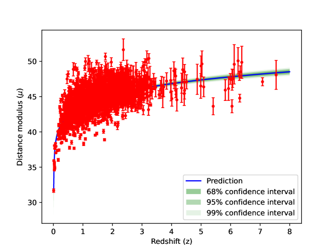
Figure 1: Reconstruction of the distance modulus of $\mu$ with GPR using X-ray and UV fluxes for 2,421 quasars.

We then construct the following linear regression relations between the six aforementioned GRB quantities in log space as follows:

$$\log\frac{L}{\operatorname{erg}\mathrm{s}^{-1}} =a_{1}+b_{1}\log\frac{\tau_{\operatorname{lag},i}}{0.1s},$$ (7)

$$\log\frac{L}{\operatorname{erg~{}s}^{-1}} =a_{2}+b_{2}\log\frac{V_{i}}{0.02},$$ (8)

$$\log\frac{L}{\operatorname{erg~{}s}^{-1}} =a_{3}+b_{3}\log\frac{E_{p,i}}{300\mathrm{keV}}$$ (9)

$$\log\frac{E_{\gamma}}{\text{ erg }} =a_{4}+b_{4}\log\frac{E_{p,i}}{300\mathrm{keV}},$$ (10)

$$\log\frac{L}{\text{ erg s }} =a_{5}+b_{5}\log\frac{\tau_{\mathrm{RT},i}}{0.1\mathrm{~{}s}},$$ (11)

$$\log\frac{E_{\text{iso }}}{\text{ erg }} =a_{6}+b_{6}\log\frac{E_{p,i}}{300\mathrm{keV}}$$ (12)

where $\tau_{\mathrm{RT},i}=\tau_{\mathrm{RT}}/(1+z)$, $\tau_{\operatorname{lag},i}=\tau_{\operatorname{lag}}/(1+z)$, $V_{i}=V(1+z)$ and $E_{p},i=E(1+z)$.

To get the best-fit parameters for each of the above equations, we apply the D’Agostini’s likelihood which incorporates errors in both the ordinate and abscissa D’Agostini (2005):

$$\mathcal{L}\left(\sigma_{\mathrm{int}},a,b\right)\propto\prod_{i}\frac{1}{\sqrt{\sigma_{\mathrm{int}}^{2}+\sigma_{yi}^{2}+b^{2}\sigma_{xi}^{2}}}\times\exp\left[-\frac{\left(y_{i}-a-bx_{i}\right)^{2}}{2\left(\sigma_{\mathrm{int}}^{2}+\sigma_{yi}^{2}+b^{2}\sigma_{xi}^{2}\right)}\right],$$ (13)

where $x$ and $y$ denote the abscissa and ordinate and $\sigma_{xi}$ and $\sigma_{yi}$ are the corresponding errors; $\sigma_{\mathrm{int}}$ denotes the intrinsic scatter in each regression relation. To get the best-fit values of each of the parameters, we do Bayesian regression and sample the posterior using the emcee MCMC sampler Foreman-Mackey et al. (2013).

In order to test if the aforementioned correlations vary with redshift, similar to Tang et al. (2021), we bifurcate the GRB datset into two subsamples corresponding to the following redshift bins: the low-z sample ($z\leq 1.4$) which consists of 50 GRBs, and the high-z sample ($z>1.4$) which consists of 66 GRBs. We investigate the redshift dependence of luminosity correlations for these two subsamples. We also show the results for the full GRB sample.

The best-fit intervals at 68%, 90%, and 99% credible intervals for all six regression relations can be found in Fig. 2 for the full GRB sample as well as after bifurcating the sample based on redshift. The scatter plots between the six pairs of variables along with the best-fits are shown in Fig. 3. We find that our results for the slope, intercept and intrinsic scatter for almost all the six scaling relations are consistent with that obtained in T21. The only exception is the $E_{p}-E_{\gamma}$ or Amati correlation, where we see an intrinsic scatter of 26-40%, whereas the intrinsic scatter was found to be $<23\%$ in T21. We find that the values for the slope and intercept are consistent or at most $1-2\sigma$ discrepant between the low redshift and high redshift samples indicating negligible evolution of the scaling relations. Furthermore, all the six regression relations show a high intrinsic scatter of greater than 30%. This includes the Amati relation, where we get a large scatter of 47%, when we consider the full data sample, similar to our results of using galaxy clusters as distance anchors Govindaraj and Desai (2022). Therefore, the regression relations between these observables cannot be used as model-independent probes of cosmological parameters.

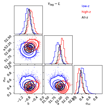
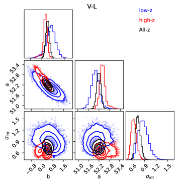
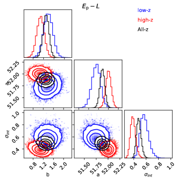
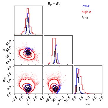
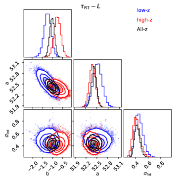
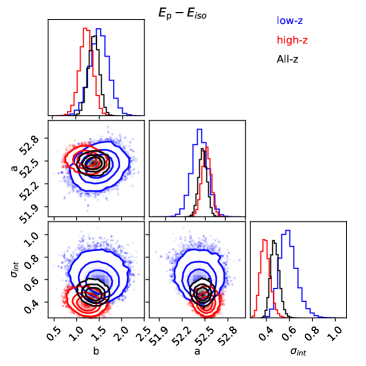
Figure 2: The 68%,90%, and 99% credible intervals along with the marginalized PDFs for the parameters for the regression relations between six pairs of GRB observables for low redshift ($z<1.4$), high redshift ($z>1.4$) as well as the full GRB dataset.

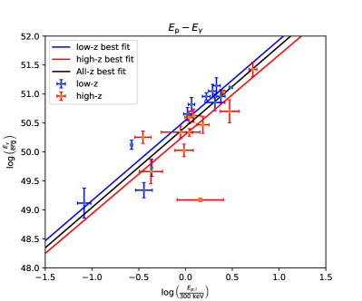
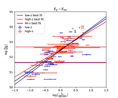
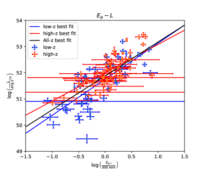
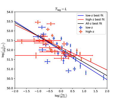
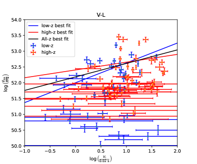
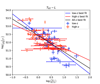
Figure 3: The luminosity correlations for low-$z$ (blue dots) and high-$z$ (red dots) GRBs. Error bars denote the 1$\sigma$ uncertainties. The lines depict the best-fit results, blue line for low-$z$ GRBs, red line for high-$z$ GRBs and black line for all-$z$ GRBs.

Table 1: The best-fitting parameters of GRB luminosity correlations. $N$ is the number of GRBs in each subsample.

Correlation	Sample	N	$a$	$b$	$\sigma_{\rm int}$
$\tau_{\rm lag}-L$	low-z	37	51.97$\pm$0.09	-0.77$\pm$0.14	0.44$\pm$0.07
	high-z	32	52.14$\pm$0.07	-0.59$\pm$0.12	0.35$\pm$0.06
	All-z	69	52.04$\pm$0.06	-0.69$\pm$0.09	0.39$\pm$0.04
$V-L$	low-z	47	52.00$\pm$0.24	0.63$\pm$0.36	0.88$\pm$0.13
	high-z	57	52.41$\pm$0.18	0.25$\pm$0.17	0.63$\pm$0.07
	All-z	104	52.19$\pm$0.12	0.43$\pm$0.13	0.73$\pm$0.06
$E_{p}-L$	low-z	50	51.75$\pm$0.09	1.38$\pm$0.18	0.58$\pm$0.07
	high-z	66	51.99$\pm$0.06	1.08$\pm$0.15	0.39$\pm$0.04
	All-z	116	51.88$\pm$0.05	1.29$\pm$0.11	0.48$\pm$0.04
$E_{p}-E_{\gamma}$	low-z	12	50.55$\pm$0.09	1.39$\pm$0.20	0.26$\pm$0.09
	high-z	12	50.30$\pm$0.14	1.37$\pm$0.44	0.39$\pm$0.16
	All-z	24	50.43$\pm$0.07	1.39$\pm$0.17	0.29$\pm$0.07
$\tau_{\rm RT}-L$	low-z	39	52.52$\pm$0.12	-1.24$\pm$0.18	0.46$\pm$0.06
	high-z	40	52.38$\pm$0.08	-0.75$\pm$0.17	0.42$\pm$0.06
	All-z	79	52.42$\pm$0.07	-1.02$\pm$0.11	0.43$\pm$0.041
$E_{p}-E_{\rm iso}$	low-z	40	52.43$\pm$0.10	1.49$\pm$0.20	0.59$\pm$0.08
	high-z	61	52.51$\pm$0.06	1.22$\pm$0.14	0.39$\pm$0.04
	All-z	101	52.47$\pm$0.05	1.38$\pm$0.12	0.48$\pm$0.04

IV Conclusions

In a recent work, T21 tested the empirical correlations among six pairs of GRB observables for 116 long GRBs (first considered in  Wang et al. (2011)) in order to test their efficacy as a cosmological probe. However, one needs an estimate of the luminosity distance, which depends on an underlying cosmological model to calculate some of these GRB observables. In order to get around this circularity problem, luminosity distances from Type Ia supernovae were used as distance anchors, and the corresponding distance at a given GRB redshift was obtained using ANN based regression.

In this work, we carry out the same exercise as T21, but use X-ray and UV fluxes of quasars instead of Type Ia supernovae in order to get the luminosity distance at a given GRB redshift. The interpolation has been done using Gaussian process regression. Similar to  Tang et al. (2021), we test the correlations for both the low redshift and high redshift sample, after bifurcating the dataset at $z=1.4$. Our results for the best-fit values for all the six regression relations can be found in Table 1. The marginalized credible intervals are shown in Fig. 2, whereas the scatter plots for the six regression relations are shown in Fig. 3. Our conclusions are as follows:

• Our slopes and intercepts agree with the corresponding results with T21 for both the low and high redshift as well as the full sample.

• Our intrinsic scatter for almost all the scaling relations are comparable to that found in T21. The only exception is the Amati relation where we see a much higher intrinsic scatter compared to T21.

• Although there is negligible redshift evolution in the scaling relations, the high intrinsic scatter implies that we cannot use these observables for model-independent estimate of cosmological parameters.

References

- Tang et al. (2021) L. Tang, X. Li, H.-N. Lin, and L. Liu, Astrophys. J. 907, 121 (2021), eprint 2011.14040.
- Kumar and Zhang (2015) P. Kumar and B. Zhang, Phys. Rep. 561, 1 (2015), eprint 1410.0679.
- Yu et al. (2022) Y.-W. Yu, H. Gao, F.-Y. Wang, and B.-B. Zhang, in Handbook of X-ray and Gamma-ray Astrophysics. Edited by Cosimo Bambi and Andrea Santangelo (2022), p. 31.
- Singh and Desai (2022) A. Singh and S. Desai, JCAP 2022, 010 (2022), eprint 2108.00395.
- Desai (2023) S. Desai, arXiv e-prints arXiv:2303.10643 (2023), eprint 2303.10643.
- Kouveliotou et al. (1993) C. Kouveliotou, C. A. Meegan, G. J. Fishman, N. P. Bhat, M. S. Briggs, T. M. Koshut, W. S. Paciesas, and G. N. Pendleton, Astrophys. J. Lett. 413, L101 (1993).
- Woosley and Bloom (2006) S. E. Woosley and J. S. Bloom, Ann. Rev. Astron. Astrophys. 44, 507 (2006), eprint astro-ph/0609142.
- Nakar (2007) E. Nakar, Phys. Rep. 442, 166 (2007), eprint astro-ph/0701748.
- Kulkarni and Desai (2017) S. Kulkarni and S. Desai, Astrophysics & Space Sciences 362, 70 (2017), eprint 1612.08235.
- Bhave et al. (2022) A. Bhave, S. Kulkarni, S. Desai, and P. K. Srijith, Astrophysics & Space Sciences 367, 39 (2022), eprint 1708.05668.
- Dainotti and Amati (2018) M. G. Dainotti and L. Amati, PASP 130, 051001 (2018), eprint 1704.00844.
- Parsotan and Ito (2022) T. Parsotan and H. Ito, Universe 8, 310 (2022), eprint 2204.09729.
- Dainotti and Del Vecchio (2017) M. G. Dainotti and R. Del Vecchio, New Astronomy Reviews 77, 23 (2017), eprint 1703.06876.
- Luongo and Muccino (2023) O. Luongo and M. Muccino, Mon. Not. R. Astron. Soc. 518, 2247 (2023), eprint 2207.00440.
- Dainotti et al. (2022) M. G. Dainotti, V. Nielson, G. Sarracino, E. Rinaldi, S. Nagataki, S. Capozziello, O. Y. Gnedin, and G. Bargiacchi, Mon. Not. R. Astron. Soc. 514, 1828 (2022), eprint 2203.15538.
- Pradyumna and Desai (2022) S. Pradyumna and S. Desai, Journal of High Energy Astrophysics 35, 77 (2022), eprint 2204.03363.
- Moresco et al. (2022) M. Moresco, L. Amati, L. Amendola, S. Birrer, J. P. Blakeslee, M. Cantiello, A. Cimatti, J. Darling, M. Della Valle, M. Fishbach, et al., Living Reviews in Relativity 25, 6 (2022), eprint 2201.07241.
- Khadka et al. (2021) N. Khadka, O. Luongo, M. Muccino, and B. Ratra, JCAP 2021, 042 (2021), eprint 2105.12692.
- Govindaraj and Desai (2022) G. Govindaraj and S. Desai, JCAP 2022, 069 (2022), eprint 2208.00895.
- Wang et al. (2011) F.-Y. Wang, S. Qi, and Z.-G. Dai, Mon. Not. R. Astron. Soc. 415, 3423 (2011), eprint 1105.0046.
- Amati (2006) L. Amati, Mon. Not. R. Astron. Soc. 372, 233 (2006), eprint astro-ph/0601553.
- Scolnic et al. (2018) D. M. Scolnic, D. O. Jones, A. Rest, Y. C. Pan, R. Chornock, R. J. Foley, M. E. Huber, R. Kessler, G. Narayan, A. G. Riess, et al., Astrophys. J. 859, 101 (2018), eprint 1710.00845.
- Dai et al. (2021) Y. Dai, X.-G. Zheng, Z.-X. Li, H. Gao, and Z.-H. Zhu, Astron. & Astrophys. 651, L8 (2021), eprint 2111.05544.
- Demianski et al. (2017a) M. Demianski, E. Piedipalumbo, D. Sawant, and L. Amati, Astron. & Astrophys. 598, A112 (2017a), eprint 1610.00854.
- Demianski et al. (2017b) M. Demianski, E. Piedipalumbo, D. Sawant, and L. Amati, Astron. & Astrophys. 598, A113 (2017b), eprint 1609.09631.
- Schaefer (2007) B. E. Schaefer, Astrophys. J. 660, 16 (2007), eprint astro-ph/0612285.
- Sari et al. (1999) R. Sari, T. Piran, and J. P. Halpern, Astrophys. J. Lett. 519, L17 (1999), eprint astro-ph/9903339.
- Mortlock et al. (2011) D. J. Mortlock, S. J. Warren, B. P. Venemans, M. Patel, P. C. Hewett, R. G. McMahon, C. Simpson, T. Theuns, E. A. Gonzáles-Solares, A. Adamson, et al., Nature (London) 474, 616 (2011), eprint 1106.6088.
- Risaliti and Lusso (2019) G. Risaliti and E. Lusso, Nature Astronomy 3, 272 (2019), eprint 1811.02590.
- Lusso et al. (2020) E. Lusso, G. Risaliti, E. Nardini, G. Bargiacchi, M. Benetti, S. Bisogni, S. Capozziello, F. Civano, L. Eggleston, M. Elvis, et al., Astron. & Astrophys. 642, A150 (2020), eprint 2008.08586.
- Seikel et al. (2012) M. Seikel, C. Clarkson, and M. Smith, JCAP 2012, 036 (2012), eprint 1204.2832.
- Singirikonda and Desai (2020) H. Singirikonda and S. Desai, European Physical Journal C 80, 694 (2020), eprint 2003.00494.
- Bora and Desai (2021a) K. Bora and S. Desai, JCAP 2021, 052 (2021a), eprint 2104.00974.
- Bora and Desai (2021b) K. Bora and S. Desai, European Physical Journal C 81, 296 (2021b), eprint 2103.12695.
- Bora et al. (2022) K. Bora, R. F. L. Holanda, S. Desai, and S. H. Pereira, European Physical Journal C 82, 17 (2022), eprint 2106.15805.
- Agrawal et al. (2021) R. Agrawal, H. Singirikonda, and S. Desai, JCAP 2021, 029 (2021), eprint 2102.11248.
- Mendonça et al. (2021a) I. E. C. R. Mendonça, K. Bora, R. F. L. Holanda, S. Desai, and S. H. Pereira, JCAP 2021, 034 (2021a), eprint 2109.14512.
- Mendonça et al. (2021b) I. E. C. R. Mendonça, K. Bora, R. F. L. Holanda, and S. Desai, JCAP 2021, 084 (2021b), eprint 2107.14169.
- Holanda et al. (2022) R. F. L. Holanda, K. Bora, and S. Desai, European Physical Journal C 82, 526 (2022), eprint 2105.10988.
- Pedregosa et al. (2011) F. Pedregosa, G. Varoquaux, A. Gramfort, V. Michel, B. Thirion, O. Grisel, M. Blondel, P. Prettenhofer, R. Weiss, V. Dubourg, et al., Journal of Machine Learning Research 12, 2825 (2011).
- D’Agostini (2005) G. D’Agostini, arXiv e-prints physics/0511182 (2005), eprint physics/0511182.
- Foreman-Mackey et al. (2013) D. Foreman-Mackey, D. W. Hogg, D. Lang, and J. Goodman, Publ. Astron. Soc. Pac. 125, 306 (2013), eprint 1202.3665.