From chiral EFT to perturbative QCD: a Bayesian model mixing approach to symmetric nuclear matter

Abstract

Constraining the equation of state (EOS) of strongly interacting, dense matter is the focus of intense experimental, observational, and theoretical effort. Chiral effective field theory ($\chi$EFT) can describe the EOS between the typical densities of nuclei and those in the outer cores of neutron stars while perturbative QCD (pQCD) can be applied to properties of deconfined quark matter, both with quantified theoretical uncertainties. However, describing the complete range of densities between nuclear saturation and an almost-free quark gas with a single EOS that has well-quantified uncertainties is a challenging problem. In this work, we argue that Bayesian multi-model inference from $\chi$EFT and pQCD can help bridge the gap between the two theories: we combine the Gaussian random variables that constitute the theories’ predictions for the pressure as a function of the density in symmetric nuclear matter. We do this using two Bayesian model mixing procedures: a pointwise approach, and a correlated approach implemented via a Gaussian Process (GP), and present results for the pressure and speed of sound in each. The second method produces a smooth $\chi$EFT-to-pQCD EOS. Without input data in the intermediate region, the choice of prior on the EOS, encoded through the GP kernel, significantly affects the result in that region. We also discuss future extensions and applications to neutron star matter guided by recent EOS constraints from nuclear theory, nuclear experiment, and multi-messenger astronomy.

I Motivation

Recent years have seen major observational, theoretical, and experimental improvements in the constraints on the cold dense matter equation of state (EOS). These advances come, e.g., from multi-messenger astronomy Vitale (2021); Corsi et al. (2024); Koehn et al. (2024), nuclear forces derived from chiral effective field theory ($\chi$EFT) and their implementation in modern many-body frameworks Hammer et al. (2020); Tews et al. (2020); Hergert (2020); Drischler et al. (2021a), Bayesian quantification of $\chi$EFT truncation uncertainties Melendez et al. (2019); Drischler et al. (2020a, b), and novel experimental campaigns such as PREX–II/CREX Adhikari et al. (2021, 2022) and heavy-ion collisions Sorensen et al. (2024); Kumar et al. (2023). Computational progress has been facilitated by emulators that can rapidly explore how aspects of $\chi$EFT nuclear forces affect the properties of nuclear matter Melendez et al. (2022); Drischler et al. (2023); Jiang et al. (2022); Duguet et al. (2023). In addition, perturbative Quantum Chromodynamics (pQCD) calculations of cold strongly interacting matter have seen major advances in the past several years: all but one of the several pieces of the $\mathcal{O}(\alpha_{s}^{3})$ contribution to the expansion in the strong coupling constant $\alpha_{s}$ of the pressure have been computed Gorda et al. (2023a, b, 2021a, 2018) and the uncertainty due to higher-order terms in the perturbative series quantified Gorda et al. (2023c). These pQCD results delineate the properties of strongly interacting matter, but only at densities far beyond those of neutron stars. Indeed, neither $\chi$EFT nor pQCD gives direct access to the EOS at the densities reached in the inner cores of neutron stars.

Nevertheless, Quantum Chromodynamics (QCD), the theory of strong interactions, describes strongly interacting matter across all relevant densities. Bayesian model mixing (BMM) enables statistically principled combination of the predictions for the EOS as computed in the EFT of QCD at nuclear densities, $\chi$EFT, and the pQCD EOS. In this article, we demonstrate how BMM can be used to construct this combination by applying it to the EOS of isospin symmetric matter at zero temperature. More generally, our BMM framework is applicable to the mixing of calculations of the nuclear EOS that have well-quantified uncertainties. It could be applied at different values of the neutron-proton excesses, finite temperatures, etc. As such, this approach can ensure full advantage is taken of the advances listed above, by formulating global microscopic EOS models covering all densities probed by neutron stars NP3M Collab. (2024); Kumar et al. (2023), with fully quantified uncertainties. Such models are a crucial input to large-scale simulations of supernovae and mergers that shed light on the synthesis of heavy nuclei and the structure and evolution of neutron stars in the universe from first principles N3AS Collab. (2024).

BMM is a class of statistical methods that combine outputs from individual models using weights that depend on the location in the input space of the problem Coleman (2019); Yao et al. (2021); Semposki et al. (2022); Yannotty et al. (2023). Here, we reiterate and then generalize the model mixing described in Refs. Phillips et al. (2021); Semposki et al. (2022). This procedure combines Gaussian random variables that represent the different models—including their error structure—thereby yielding information on the theory underlying both models. The combination can be made pointwise Phillips et al. (2021); Semposki et al. (2022), but the more sophisticated approach adopted here produces a representation of that underlying theory as a set of Gaussian random variables that are correlated across the input space, i.e., a Gaussian process (GP). GPs are now a standard tool for nonparametric EOS modeling in neutron-star applications Essick et al. (2020); Mroczek et al. (2023), but while previous work has emphasized their model-agnostic benefits, here we inform our EOS GP using the low- and high-density limits of QCD. This is an example of BMM in which Gaussian random variables are combined, but other versions involve combining means and adjusting the variance to data Yannotty et al. (2023); Kejzlar et al. (2023), or forming linear combinations of the probability distribution functions obtained in the individual models Coleman (2019); Yao et al. (2021).

Our specific implementation of BMM and its application to symmetric two-flavor strongly interacting matter is described in what follows. Detailed descriptions of the $\chi$EFT and pQCD equations of state at fixed number density $n$ are presented in Sec. II, as is a determination of the truncation uncertainties in both theories. Subsection II.4 then discusses other theoretical information on the EOS that could be incorporated in our mixing. The two BMM approaches investigated in this work are described in Secs. III and IV, and results for the two methods are detailed in the respective sections. We summarize and discuss the implications of our findings for future work in Sec. V. Appendix A discusses how we obtain the pQCD pressure as a function of the baryon density using the Kohn-Luttinger-Ward formalism Kohn and Luttinger (1960); Luttinger and Ward (1960), and Appendix B details how we compute the pQCD speed of sound at a given density consistently up to a finite order in $\alpha_{s}$. Our software implementation, including annotated Jupyter notebooks used to produce the results in this paper, will be made publicly available in a GitHub repository. Throughout the paper, we use natural units in which $\hbar=c=1$.

II Dense matter equations of state

In this section, we discuss the microscopic calculations at low ($\chi$EFT in Subsec. II.2) and high (pQCD in Subsec. II.3) densities. But first we discuss how we use well-developed machinery for assessing truncation errors of finite perturbation series to quantify each theory’s uncertainties (Subsec. II.1). These calculations become input for multiple-model Bayesian inference (Secs. III and IV). Subsection II.4 discusses other theoretical approaches for the dense-matter EOS whose results could potentially be added to the inference.

II.1 Uncertainty quantification using the BUQEYE truncation error model

Uncertainty quantification (UQ) is a critical component of microscopic EOS modeling. In this work, we follow the UQ methodology developed in Ref. Melendez et al. (2019) and use correlated truncation error estimation to accurately obtain our model uncertainties for each EOS investigated.

We begin by considering our theories as observables $y(x)$ calculated as a function of the input parameter $x$, which could be the Fermi momentum, the associated density or chemical potential of the matter under consideration. We assume the corresponding $y$ has an expansion in powers of a small parameter $Q(x)$, and then express the cumulative result at the $k$th order in that expansion, $y_{k}(x)$, as

$$y_{k}(x)=y_{\textrm{ref}}(x)\sum_{n=0}^{k}c_{n}(x)Q^{n}(x),$$ (1)

where $y_{\textrm{ref}}(x)$ is a dimensionful reference scale of the theory that sets the typical size of the observable, and $c_{n}(x)$ are the corresponding coefficients at each order. We will make separate choices for $Q(x)$ and $y_{\textrm{ref}}(x)$ for each of the two EOSs considered in this work, in each case choosing these aspects of the expansion based on the convergence properties and nominal expansion parameters of the respective theories.

We desire to quantify truncation uncertainties up to $y_{\infty}$, based on the convergence pattern of the $n\leq k$ orders we possess. To do this, we will need to estimate the impact of orders $n>k$ in our expansion. We first extract the coefficients $c_{n}(x)$ at each known order, by employing the relations

$$y_{0}(x) \equiv y_{\textrm{ref}}(x)c_{0}(x),$$ (2)

$$\Delta y_{n}(x) \equiv y_{\textrm{ref}}(x)c_{n}(x)Q^{n}(x),$$ (3)

where we calculate the correction to $y(x)$ at $n^{th}$ order in Eq. (3). We can then estimate higher orders based on the lower order coefficients by writing the series expansion for truncated orders as

$$\delta y_{k}(x)=y_{\textrm{ref}}(x)\sum_{n=k+1}^{\infty}c_{n}(x)Q^{n}(x).$$ (4)

We have previously defined $y_{\textrm{ref}}(x)$ and $Q(x)$, so we only need to find the coefficients in Eq. (4). Since information on the overall size of the observable and the expansion’s convergence is encoded in these quantities, the different coefficients $c_{n}(x)$ should all be of a similar, $\mathcal{O}(1)$ size. We assume that the $c_{n}(x)$ curves for $n\leq k$ that we already know via Eq. (3) are independent draws from a Gaussian process (GP). We then make the inductive step that all higher $c_{n}(x)$ are also drawn from the same GP distribution.

Gaussian processes can be described as a collection of random variables, any subset of which possesses a joint Gaussian distribution Melendez et al. (2019); Rasmussen and Williams (2006). The GPs we use here can be written as

$$c_{n}(x)\sim\mathcal{GP}[0,\bar{c}^{2}r(x,x^{\prime};\ell)],$$ (5)

and are composed of a mean function (which we take to be zero) and a positive semi-definite covariance function, $\bar{c}^{2}r(x,x^{\prime};\ell)$, which is often referred to as the kernel. Kernels are parameterized by a correlation structure $r(x,x^{\prime};\ell)$ and a marginal variance $\bar{c}^{2}$. These encode the correlations in the dataset and the variability of the data from the mean, respectively. The marginal variance and correlation structure inferred from $\{c_{n}(x),n\leq k\}$ are then, by assumption, inherited by the uncomputed coefficients that define the missing higher orders in the expansion. For more details on the mathematics of GPs, we refer the reader to Rasmussen and Williams (2006); Melendez et al. (2019).

For both EOSs discussed in the following sections, the stationary, radial basis function (RBF) kernel is chosen as the kernel for the truncation-error model. This kernel is described by

$$r(x,x^{\prime};\ell)=\exp[-\frac{(x-x^{\prime})^{2}}{2\ell^{2}}\bigg{]},$$ (6)

which builds in a strict assumption of smoothness for the $c_{n}(x)$ across the input space—the RBF kernel is infinitely differentiable. This choice also builds in an assumption of stationarity in our input space—the RBF kernel only depends on the relative distance between points in the input space, not on the actual locations of the points themselves.

As a prior on $\bar{c}^{2}$, we choose the scaled inverse $\chi^{2}$ distribution. This is a conjugate prior for the variance of the Gaussian distribution, and so is straightforwardly updated using the $c_{n}(x)$ coefficients through updating equations for the degrees of freedom $\nu$ and scale $\tau$ of the scaled inverse $\chi^{2}$. The choice of hyperparameters ($\nu_{0}$ and $\tau_{0}^{2}$), together with other options, are discussed in Melendez et al. (2019).

The correlations of the $c_{n}(x)$ across $x$ induces correlations in the truncation error $\delta y_{k}$ across $x$. This desirable feature can be incorporated naturally into the model mixing procedure, where mean predictions $y_{k}(x)$ and their errors $\delta y_{k}(x)$ become the training data. Correlated error structures in this training data stop the mixed model from overweighting information that is actually redundant.

II.2 Low-density EOS from chiral EFT ($\chi$EFT)

At low densities ($n\lesssim 2n_{0}$), where QCD is highly nonperturbative, $\chi$EFT  provides a systematic expansion for nuclear forces; its expansion parameter is the ratio of the typical momentum of the system and the $\chi$EFT breakdown scale $\Lambda_{b}\approx 600\,\text{MeV}$ Epelbaum et al. (2015); Drischler et al. (2020a); Millican et al. (2024). We assert the Fermi momentum as the typical momentum of low-density nuclear matter.

We use here the predictions of $\chi$EFT up to N³LO for the energy per particle, $E(n)/A$, obtained using fourth-order many-body perturbation theory (MBPT) in Refs. Drischler et al. (2019); Leonhardt et al. (2020). The (nonlocal) chiral interactions consisted of the family of order-by-order NN potentials developed by Entem, Machleidt, and Nosyk Entem et al. (2015) and 3N forces at the same order in the chiral expansion and with the same momentum cutoff (see Table I of Ref. Drischler et al. (2020a) for more details). The 3N low-energy constants (LECs) $c_{D}$ and $c_{E}$ were fit to the triton binding energy and adjusted to the empirical nuclear saturation point in symmetric nuclear matter Drischler et al. (2019). However, we stress that the BUQEYE truncation error framework, discussed in Sec. II.1, can be applied to any order-by-order calculations in the EFT expansion, independent of the computational framework used to solve the many-body Schrödinger equation and the details of the order-by-order EFT interactions.

Throughout this work, we assume both NN and 3N LECs to be fixed to the values obtained by the developers of the nuclear potentials. Specifically, we focus on the pressure from $\chi$EFT up to N³LO (i.e., $k\leqslant 4$), obtained as the (rescaled) density derivative of $E(n)/A$, for the interactions with the momentum cutoff $\Lambda=500\,\text{MeV}$. We use these results from Ref. Drischler et al. (2020a), in which the BUQEYE truncation error model was used to quantify correlated EFT truncation errors and propagate them to derivative quantities such as the pressure.

This was done by first choosing the variable in which the GP would be constructed. For this EOS, this is the Fermi momentum $k_{F}$, as this choice was superior to the density $n$ in terms of stationarity of the coefficients’ correlation structure Drischler et al. (2020a).

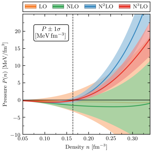
Figure 1: Order-by-order results, including $1\sigma$ uncertainty bands, for the pressure of the isospin-symmetric matter EOS from $\chi$EFT, with an NN potential cutoff of $\Lambda=500$ MeV. The black dashed line indicates the saturation density, $n_{0}=0.164$ fm^-3 Drischler et al. (2016). Figure code adapted from Jupyter notebooks published with Refs. Drischler et al. (2020a, b).

$y_{\textrm{ref}}$ was chosen to be

$$y_{\textrm{ref}}(k_{F})=16\,\text{MeV}\times\left(\frac{k_{F}}{k_{F,0}}\right)^{2},$$ (7)

which was motivated by the structure of the $\chi$EFT leading order (LO) term and empirical knowledge of the nuclear saturation point in SNM. Note here that $k_{F,0}\approx 1.344~{}\textrm{fm}^{-1}$ is the Fermi momentum at the saturation density $n_{0}=n(k_{F,0})\approx 0.164\,\text{fm}^{-3}$ Drischler et al. (2016), with $n(k_{F})=2k_{F}^{3}/(3\pi^{2})$, and $|E(n_{0})/A|\approx 16\,\text{MeV}$ the corresponding absolute value of the saturation energy in SNM. To employ Eq. (1), an expansion parameter $Q$ must also be specified; Ref. Drischler et al. (2020a) chose

$$Q(k_{F})=\frac{k_{F}}{\Lambda_{b}},$$ (8)

where $\Lambda_{b}$ is the breakdown scale, estimated to be $\Lambda_{b}\approx 600\,\text{MeV}$ as previously mentioned.

Results for the pressure of symmetric nuclear matter, $P(n)$, are obtained using

$$P(n)=n^{2}\derivative{n}\frac{E}{A}(n),$$ (9)

see Fig. 1, which also shows combined quantified truncation and GP interpolation uncertainties for the prediction of the EFT at each known order. Equation (9) and Fig. 1 are shown in terms of the number density, $n$—we will perform multi-model Bayesian inference in this input space.

To construct the error bands, the scaled inverse $\chi^{2}$ priors on $\bar{c}$ and $\ell$ discussed in the previous section were used, with degrees of freedom $\nu_{0}=10$ and scale parameter $\tau_{0}^{2}=(\nu_{0}-2)/\nu_{0}$ to enforce the condition of naturalness of the known coefficients $c_{n}(x)$. A white noise kernel was added to the RBF kernel to account for the higher-order uncertainty from the MBPT calculations (see Ref. Drischler et al. (2020a) for more details). The 68% (i.e., $1\sigma$) intervals in Fig. 1 indicate good convergence properties at each order around and below $n_{0}$. We point out that though the N³LO band may appear wider than the N²LO band at densities $\simeq 2n_{0}$, this is not the case when comparing the size of these uncertainty bands numerically.

With $P(n)$ and $E(n)/A$ in hand, we compute the speed of sound from

$$c_{s}^{2}(n)=\frac{\partial P}{\partial\varepsilon}=\frac{\partial P}{\partial n}\left(\frac{\partial\varepsilon}{\partial n}\right)^{-1},$$ (10)

where $\varepsilon(n)=n\left[E(n)/A+m_{N}\right]$ is the energy density with the nucleon rest-mass ($m_{N}$) contribution. To properly propagate the correlated uncertainties to the sound speed, we sample curves from $E(n)/A$ and compute derivatives that preserve the aforementioned correlations. Figure 2 shows the corresponding results order-by-order through N³LO.

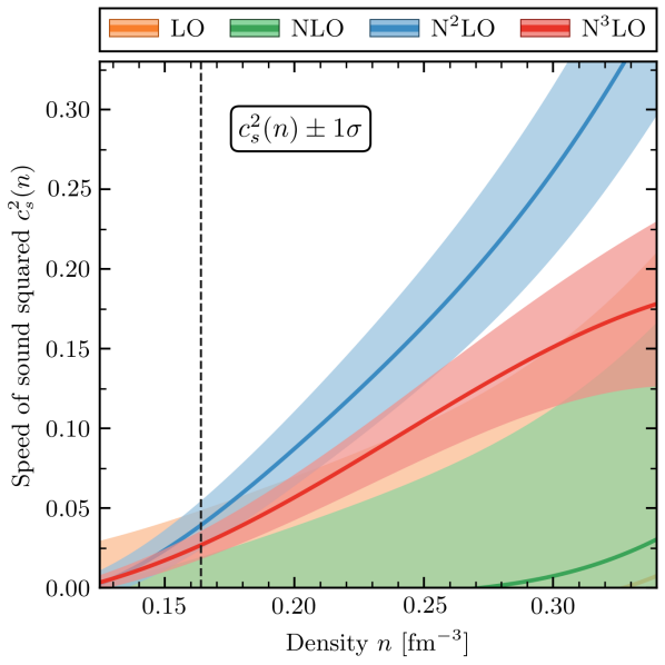
Figure 2: Speed of sound squared results for symmetric matter from $\chi$EFT, sampling directly from $E(n)/A$. The black dashed line indicates the saturation density of $n_{0}=0.164$ fm^-3. We only plot above where $c_{s}^{2}(n)=0$, as a negative sound speed indicates unstable matter. Figure code adapted from Jupyter notebooks published with Refs. Drischler et al. (2020a, b).

II.3 High-density EOS from perturbative QCD (pQCD)

At very high densities ($n\gg 2n_{0}$), QCD becomes perturbative due to asymptotic freedom, and thus can be expanded in the strong coupling constant, $\alpha_{s}$, which we take at the two-loop level to be Kurkela et al. (2010); Zyla et al. (2020)

$$\alpha_{s}(\bar{\Lambda})=\frac{4\pi}{\beta_{0}L}\left[1-\frac{2\beta_{1}}{\beta_{0}^{2}}\frac{\ln{L}}{L}\right],$$ (11)

with

$$L = \ln({\bar{\Lambda}^{2}/\Lambda_{\overline{MS}}^{2}}),\quad\bar{\Lambda}=2X\mu,$$

$$\beta_{0} = 11-\frac{2}{3}N_{f},\quad\beta_{1}=51-\frac{19}{3}N_{f},$$ (12)

where we took $N_{c}=3$, and $\bar{\Lambda}$ is the renormalization scale, defined in this work to vary around the chemical potential by a factor $2X=[1,4]$. Recent Bayesian treatments of pQCD have marginalized over this unphysical parameter Gorda et al. (2023c, a); for the purposes of this proof-of-principle study we invoke the large-$N_{f}$ and phenomenological model arguments of Ref. Kurkela et al. (2010) and set $X=1$ in the main results of our study. $\Lambda_{\overline{MS}}$ has been determined via experimental constraints to be $0.38\pm 0.03$ GeV Kurkela et al. (2010). We note that, because we use this value of $\Lambda_{\overline{MS}}$ at each order of the pQCD result, we must also incorporate the two-loop running of $\alpha_{s}(\bar{\Lambda})$ throughout the calculation.

The form of pQCD EOS used here is the weak-coupling expansion of the theory through N²LO. The parameterization we choose to employ is taken from Ref Gorda et al. (2023a):

$$\frac{P(\mu)}{P_{FG}(\mu)}\simeq 1 +~{}a_{1,1}\left(\frac{\alpha_{s}(\bar{\Lambda})}{\pi}\right)$$ (13)

$$+ N_{f}\left(\frac{\alpha_{s}(\bar{\Lambda})}{\pi}\right)^{2}\bigg{[}a_{2,1}\ln\left(\frac{N_{f}\alpha_{s}(\bar{\Lambda})}{\pi}\right)$$

$$+ a_{2,2}\ln\frac{\bar{\Lambda}}{2\mu}+a_{2,3}\bigg{]}+\mathcal{O}(\alpha_{s}^{3}),$$

with coefficients $a_{1,1}=-2$, $a_{2,1}=-1$, $a_{2,2}=-4.8333$, $a_{2,3}=-8.0021$, and where $N_{f}=2$ and $N_{c}=3$ for the present system. Here, we also define the Fermi gas (FG) pressure as

$$P_{FG}(\mu)\equiv N_{c}N_{f}\frac{\mu^{4}}{12\pi^{2}}=\frac{\mu^{4}}{2\pi^{2}}.$$ (14)

In this work, we use $\mu\equiv\mu_{q}$, and denote $\mu_{B}=3\mu$ explicitly when discussing the baryon chemical potential.

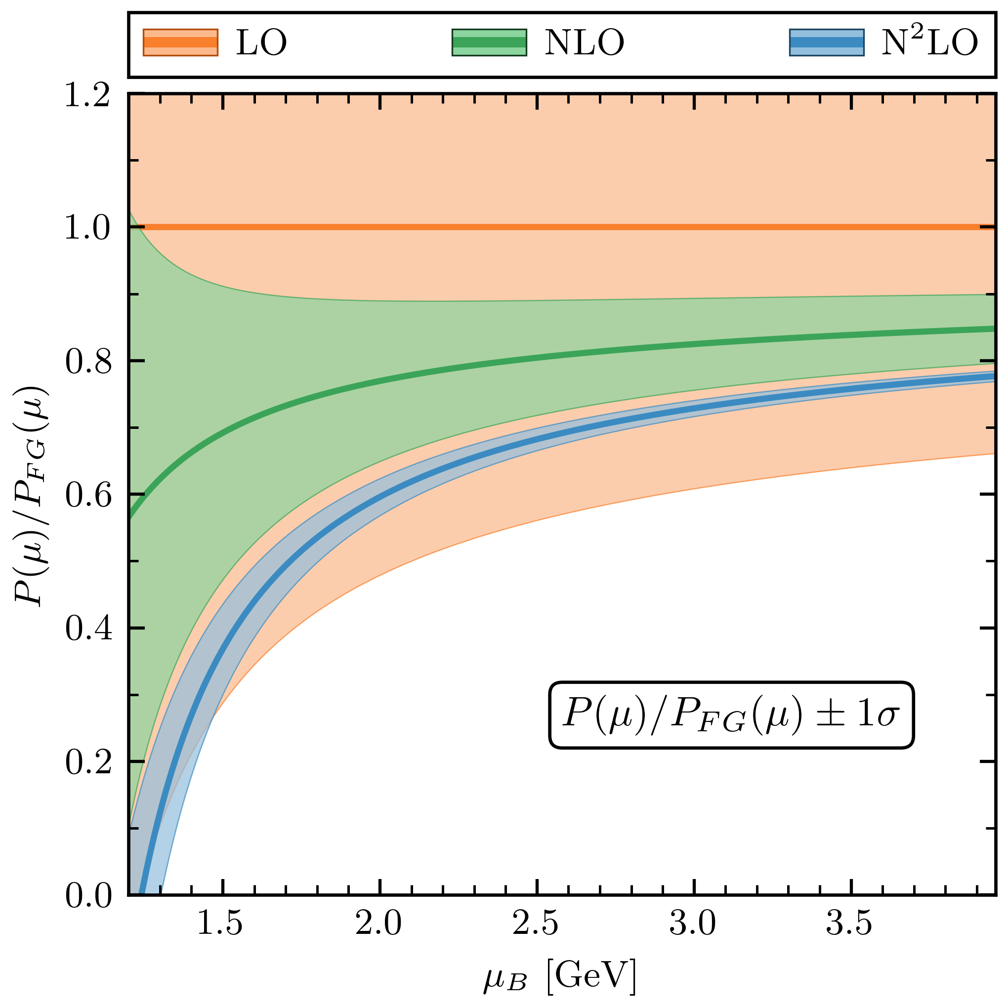
Figure 3: Order-by-order $P(\mu)$ results, scaled with the Fermi gas pressure $P_{FG}(\mu)$, for the EOS from pQCD, plotted against the baryon chemical potential $\mu_{B}=3\mu$, where $\mu\equiv\mu_{q}$. Results are shown up to and including LO, NLO, and N²LO, respectively, with $1\sigma$ truncation error bands.

To properly quantify the truncation error in the pQCD pressure $P(\mu)$, we apply the methodology of Sec. II.1 to the results of Eq. (13). We choose an expansion parameter of $Q(\bar{\Lambda})=N_{f}\alpha_{s}(\bar{\Lambda})/\pi$, and the reference scale $y_{\textrm{ref}}=P_{FG}(\mu)$, and train on the known coefficients of each order, treating them as functions of the quark chemical potential. This produces the truncation error bands shown in Fig. 3 at the $1\sigma$ level. The NLO result is well within the 68% credibility interval of the LO (Fermi gas) result, but the N²LO $P(\mu)$ curve sits between 1 and 1.5$\sigma$ away from the NLO pressure. We will take this opportunity to emphasize the point that this is not a statistically inconsistent result. Indeed, if every order fell within the previous order’s 68% credibility interval, then that would mean the expansion parameter adopted for the perturbative series was too large, and the resulting error bands too large (“conservative”).

To perform model mixing with both models in the same input space, we choose to convert the pQCD pressure, $P(\mu)$, to $P(n)$. To do this in a way that retains only terms up to $\mathcal{O}(\alpha_{s}^{2})$, we invoke the procedure of Kohn, Luttinger, and Ward Kohn and Luttinger (1960); Luttinger and Ward (1960). This procedure first inverts the expression for $n(\mu)$ consistently up to the desired order in perturbation theory, producing a series $\mu=\mu_{FG}+\mu_{1}+\mu_{2}+\ldots$ in which each $\mu_{k}$ equals $\mu_{FG}\alpha_{s}^{k}$ times a numerical coefficient. This series is then substituted into the formula for $P(\mu)$ and the result expanded again in powers of $\alpha_{s}$ and truncated at the desired order. This yields a perturbative series for $P$ in which the only chemical potential that appears is $\mu_{FG}$. Since

$$\mu_{FG}=\left(\frac{3\pi^{2}n}{N_{c}N_{f}}\right)^{1/3},$$ (15)

this means we have accomplished our goal of finding the strictly perturbative expression for the function $P(n)$. This calculation is carried out in detail in Appendix A, and up to and including $\mathcal{O}(\alpha_{s}^{2})$, it gives

$$\frac{P(n)}{P_{FG}(n)} = 1+\frac{2}{3\pi}\alpha_{s}(\bar{\Lambda}_{FG})$$ (16)

$$+ \frac{8}{9\pi^{2}}\alpha_{s}^{2}(\bar{\Lambda}_{FG})-\frac{N_{f}^{2}}{3\pi^{2}}c_{2}(\mu_{FG})\alpha_{s}^{2}(\bar{\Lambda}_{FG})$$

$$- \frac{\beta_{0}}{3\pi^{2}}\alpha_{s}^{2}(\bar{\Lambda}_{FG}),$$

where

$$c_{2}(\mu_{FG})=\frac{1}{N_{f}}\bigg{[}a_{2,1} \ln{\left(\frac{N_{f}\alpha_{s}(\bar{\Lambda}_{FG})}{\pi}\right)}$$

$$+a_{2,2}\ln{\left(\frac{\bar{\Lambda}_{FG}}{2\mu_{FG}}\right)}+a_{2,3}\bigg{]}.$$ (17)

Comparing Eqs. (16) and (13) shows that the NLO contribution to $P(n)$ has the opposite sign to that in $P(\mu)$. Consequently, the direction of approach to the asymptotic Fermi gas result in $P(n)$ is from above, rather than from below, as it is in $P(\mu)$. The NLO coefficient in $P(n)$ is also only 1/3 the size of the corresponding piece of $P(\mu)$, and the N²LO coefficient is also markedly smaller in $P(n)$. These changes in the properties of the expansion are all consequences of performing the KLW inversion from pressure at fixed chemical potential to obtain pressure at fixed number density.

Figure 4 shows our results for $P(n)$, as well as the application of the BUQEYE truncation error framework discussed in Sec. II.1. These truncation error bands are obtained by using the same expansion parameter, variance (and length scale) as in the $P(\mu)$ result, but evaluated at the quark chemical potential $\mu_{FG}$ corresponding to each desired baryon number density, Eq. (15). Because the coefficients in the expansion for $P(\mu)$ are larger than those in $P(n)$ the credibility intervals obtained by this procedure have empirical coverage probabilities that are higher than their theoretical credibility percentage.

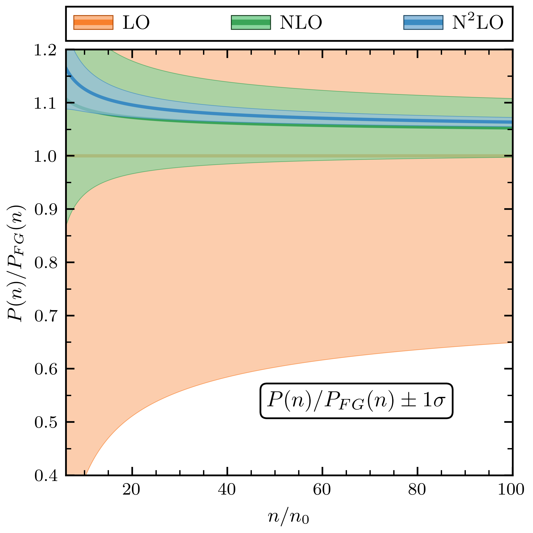
Figure 4: Order-by-order results for the pressure as a function of scaled number density $n/n_{0}$, via the KLW inversion, from the pQCD EOS.

Since, in the context of pQCD, we have $P$ as a function of chemical potential, we can compute the sound speed squared from Eq. (13), employing

$$c_{s}^{2}(\mu)=\frac{\partial P}{\partial\mu}\left(\mu~{}\frac{\partial^{2}P}{\partial\mu^{2}}\right)^{-1}.$$ (18)

Details of this calculation can be found in Appendix B. Meanwhile, Eq. (10) can be recast as

$$c_{s}^{2}(n)=n\frac{\partial\ln(\mu(n))}{\partial n},$$ (19)

through the use of $P=n\mu-\varepsilon$ and $\mu=\frac{\partial\varepsilon}{\partial n}$. In the second part of Appendix B, we use this compact form to compute $c_{s}^{2}(n)$ and find that, up to second order, it has the same functional form as $c_{s}^{2}(\mu)$. Moreover, we show that $c_{s}^{2}$ approaches its asymptotic value of $1/3$ from below, and, at large density, the deviation of this quantity from 1/3 is of $\mathcal{O}(\alpha_{s}^{2})$, with a coefficient determined purely by the running of $\alpha_{s}$. The $\mathcal{O}(\alpha_{s})$ contribution to $c_{s}^{2}$ is zero. Figure 5 plots these results for the speed of sound squared as a function of the density, together with their uncertainties. The N²LO result sits slightly below $1/3$ in the range shown here, as expected. We note that in Fig. 5 the NLO result deviates slightly from 1/3 because the speed of sound is computed using Eq. (19) here, and the derivatives of pressure in the numerical implementation of that equation induce effects of $\mathcal{O}(\alpha_{s}^{2})$ and above in the final result.

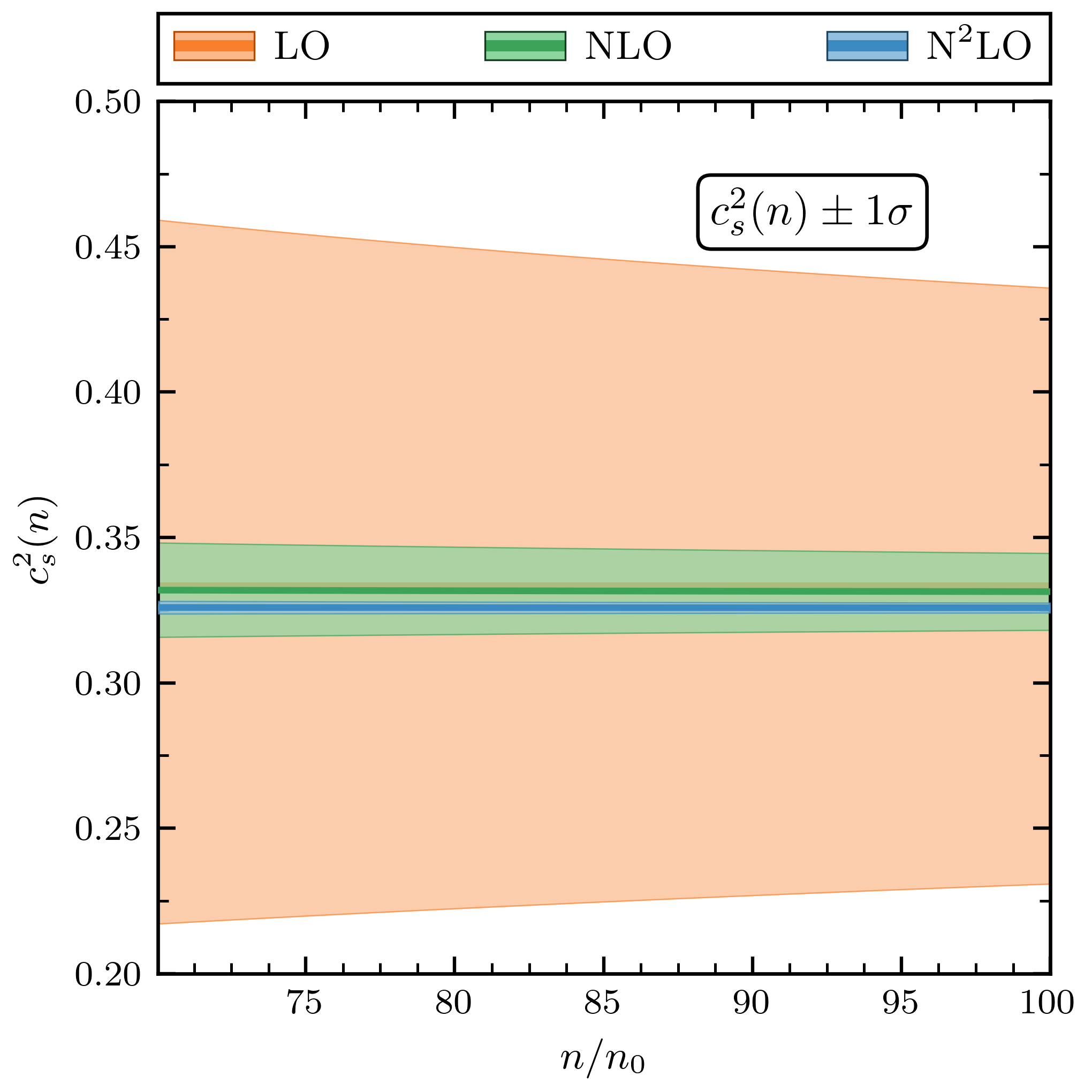
Figure 5: Order-by-order speed of sound squared results for the pQCD EOS with respect to the scaled number density $n/n_{0}$. As discussed in the main text, the result for the Fermi gas (leading order) contribution is exactly 1/3 (orange line), as expected, and the next-to-leading-order contribution (green line) is consistent with zero.

Table 1: A selection of common cutoff densities in $\chi$EFT (N³LO) at which the relative error of the pressure $P(n)$ of pQCD (N²LO) is equal. We evaluate these relative errors at $X=0.5$ and $X=1$, to illustrate the effect of changing this scale parameter.

$Q(\bar{\Lambda})$	$n/n_{0}$			Relative
	$\chi$EFT	pQCD		error (%)
		$X=1/2$	$X=1$
$\frac{N_{f}}{\pi}\alpha_{s}(\bar{\Lambda})$	1.5	17.8	2.43	33
	1.75	18.7	2.59	29
	2.0	18.9	2.62	28

Table 1 compares the size of the truncation error bands in $\chi$EFT at $n=1.5n_{0}$, $n=1.75n_{0}$, and $n=2n_{0}$ to the size of the pQCD error bands to determine where in density pQCD becomes as uncertain as $\chi$EFT is at each of those three densities. (A similar exercise was carried out in Ref. Fraga et al. (2014).) For the choice $X=1$, and taking an expansion parameter $Q(\bar{\Lambda})=\frac{N_{f}}{\pi}\alpha_{s}(\bar{\Lambda})$, this happens $0.5$–$1n_{0}$ above the $\chi$EFT density we choose for the comparison—and therefore much lower than the $(20-40)n_{0}$ that is often quoted (see, e.g., Ref. Gorda (2023)). This might lead one to believe that pQCD is applicable at neutron star densities. However, the perturbative series does not include all nonperturbative effects; for example, hadronization and pairing are not accounted for there. Once such effects become sizable, the uncertainty computed by analyzing the order-by-order behavior of pQCD will no longer encompass the full QCD result Komoltsev et al. (2023); Gorda et al. (2023c).

II.4 Other theoretical approaches to the EOS

There are, of course, several models of QCD that provide information on the EOS in the intermediate regime between $2n_{0}$ and $40n_{0}$. In principle, these can be added to our multi-model inference: the framework is easily extended to inference from more than two models. However, a model can only be added to the mix if it comes with reliable uncertainties—that preferably also have a well-understood correlation structure. In this subsection, we list QCD-based approaches to the EOS that may satisfy this condition, but which we have not yet included in our multi-model inference.

• Constraining the EOS at low densities using pQCD. The requirements that a neutron star built out of strongly interacting matter be stable and have a causal EOS have been used, together with the pQCD EOS at densities above $40n_{0}$, to construct likelihoods in the $\varepsilon-P$ plane for the strongly interacting EOS Komoltsev and Kurkela (2022); Komoltsev et al. (2023). These are not direct pQCD constraints, and not all QCD EOSs are subject to the constraints obtained in these works Mroczek et al. (2023), so we have not included them here.

• Lattice QCD constraints. QCD inequalities imply that the pressure of symmetric nuclear matter at chemical potential $\mu$ is bounded from above by the pressure of fully isospin-stretched matter at $2/3\mu$ Fujimoto and Reddy (2023). Reference Fujimoto and Reddy (2023) combined this insight with the results for the energy of a system of several thousand pions Abbott et al. (2023) to place bounds on the symmetric-matter EOS $P(\mu)$. These bounds, when interpreted as a probability distribution, are a $\theta$ function. They do not affect our multi-model inference, i.e., all EOSs we construct satisfy the bound at high credibility levels.

• Functional Renormalization Group (FRG) results. FRG attempts to truncate the hierarchy of Schwinger-Dyson equations for the $n$-point functions of QCD, by matching to pQCD at a high-resolution scale, and including non-perturbative information on those $n$-point functions at low-resolution scale Leonhardt et al. (2020); Braun et al. (2020); Braun and Schallmo (2022). Variation of the input choices in the FRG calculation provides a lower bound on its uncertainty. Results for isospin-symmetric QCD matter using this approach—including error bands—were provided in Ref. Leonhardt et al. (2020). We display these results on some of our plots, but we emphasize that the error band shown there should not be interpreted as a Bayesian credibility interval. In consequence, it is not clear to us what uncertainties to assign to these FRG calculations, and so we choose not to mix them with the pQCD and $\chi$EFT results obtained earlier in this section.

III Pointwise multivariate model mixing

In this section, we first describe the general framework for pointwise Bayesian model mixing in Sec. III.1. We then proceed to its implementation and the results obtained using this approach in Sec. III.2.

III.1 Formalism

Here, we describe the pointwise approach to Bayesian model mixing, outlined in Ref. Phillips et al. (2021) and investigated in Ref. Semposki et al. (2022). This approach is implemented in the versatile BAND collaboration BMM software package Taweret Ingles et al. (2023). Given $M$ models we wish to mix, we form

$$Y^{(i)}(x)=F(x)+\delta Y^{(i)}(x),\qquad i\in[1,M],$$ (20)

where $Y^{(i)}(x)$ is a random variable that represents the predictions at a point $x$ from a given model $i$, $F(x)$ is the underlying theory, and $\delta Y^{(i)}(x)$ represents the error of the model. In this work, $i$ denotes $\chi$EFT or pQCD, and $\delta Y^{(i)}(x)$ represents their truncation error. These distributions were modeled as Gaussian processes in Sec. II.1. In this section, we discard the information on the correlation structure of $\delta Y^{(i)}(x)$ in density and take only the diagonal elements of the theory covariance matrices derived in Secs. II.2 and II.3. We thus have

$$\delta Y^{(i)}(x)\sim\mathcal{N}[0,\sigma_{i}^{2}(x)],$$ (21)

where $\sigma_{i}(x)$ is inferred from the order-by-order convergence of each theory.

In what follows, we use a notation that concatenates the predictions and uncertainties of the different models into one vector and one matrix, respectively. We collect the set of model predictions at each point in $x$ into an $M$-dimensional vector: $\vec{y}(x)\equiv\{y_{i}(x)\}$, $i=1,\ldots,M$. The covariance matrix for these data is then denoted by $K_{y}(x)$. We take it to be diagonal: $K_{y,ij}(x)\equiv\sigma_{i}^{2}(x)\delta_{ij}$, $i,j=1,\ldots,M$, therefore assuming that the models are uncorrelated with one another. This assumption could be relaxed, without modifying any of the equations below, by extending the formalism to pointwise inter-model correlations. But, regardless of that, this approach assumes separate, independent, $M\times M$ matrices $K_{y}$ at each point $x$ for which we want to perform model mixing.

The following process is then carried out for each point $x$ in the input space. We use Bayes’ theorem to write the posterior probability distribution for the underlying theory $F$ at the point $x$:

$$\operatorname{pr}(f(x)\,|\,\vec{y}(x),K_{y}(x))\propto \operatorname{pr}(\vec{y}(x)\,|\,f(x),K_{y}(x))$$

$$\times\operatorname{pr}(f(x)).$$ (22)

Unsurprisingly, given that this is a Bayesian calculation, the prior for the underlying theory $\operatorname{pr}(f(x))$ has to be specified; here we choose

$$\operatorname{pr}(f(x))=\mathcal{N}[0,\sigma_{f}^{2}(x)],$$ (23)

where $\sigma_{f}^{2}(x)$ represents (pointwise) information we have about this theory in the chosen input space. For our present case, we will take this prior to the uninformative limit, $\sigma_{f}^{-2}(x)\rightarrow 0$.

After completing the square, the log posterior for each $f(x)$ is then, up to constant terms,

$$\log \operatorname{pr}(f(x)\,|\,\vec{y}(x),K_{y}(x))\propto$$

$$-\frac{1}{2}[f(x)-\mu(x)]^{T}\Sigma^{-1}(x)[f(x)-\mu(x)],$$ (24)

and thus $F(x)$ is Gaussian distributed,

$$\operatorname{pr}(f(x)\,|\,\vec{y}(x),K_{y}(x),\sigma_{f}^{2}(x))=\mathcal{N}[\mu(x),\Sigma(x)],\\$$ (25)

where

$$\mu(x) \equiv\Sigma(x)B^{T}K_{y}^{-1}(x)\vec{y}(x),$$

$$\Sigma(x) \equiv\left(\sigma_{f}^{-2}(x)+B^{T}K_{y}^{-1}(x)B\right)^{-1},$$ (26)

and $B=\vec{1}$ sums the elements of the object it multiplies across the space of $M$ models.

We have used two (three including the prior) Gaussian random variables that describe the input theories at the point $x$ to infer the mean and variance of the random variable $F(x)$. The combination produces a Gaussian mixed model result. Converting the results (III.1) into forms where the sum over model space is explicit we find, in the uninformative limit $\sigma_{f}^{-2}(x)\rightarrow 0$,

$$\mu(x)=\Sigma(x)\sum_{i=1}^{M}\frac{1}{\sigma_{i}^{2}(x)}y_{i}(x),\qquad\Sigma^{-1}(x)\equiv\sum_{i=1}^{M}\frac{1}{\sigma_{i}^{2}(x)}.$$ (27)

These formulae are exactly those that govern the estimation of a common mean from $M$ Gaussian-distributed measurements of different precision. The best estimate for the mean is the precision-weighted combination of the measurements, and the variance of that estimate is given by the harmonic mean of the individual measurement variances. In our case this combination of the individual model means and variances is done at each point in the input space of the problem, as previously mentioned. This allows the model with the highest precision in a given region to dominate the mixed-model in that region (see Eq. (27)).

However, this local quality of the mixing means that we need each model being mixed to have calculated values across the entire input space for both $y(x)$ and $\sigma^{2}(x)$. Due to this requirement, in our application, we need to extend the $\chi$EFT results beyond the density regime where they are typically computed and where $\chi$EFT with pion-nucleon degrees of freedom is an efficient expansion for nuclear forces in medium ($n\lesssim 2n_{0}$). Although in principle these results are needed up to $100n_{0}$, in practice the results in $\chi$EFT become irrelevant around $(5-6)n_{0}$, since the estimated pQCD error bars from the present truncation model for $P(n)$ become much smaller than the $\chi$EFT ones, rendering the $\chi$EFT weights negligible in the mixture at and beyond that density. Nevertheless, this does mean we need a robust extension of the EOS from where our $\chi$EFT results stop ($\approx 2n_{0}$).

To extrapolate the $\chi$EFT GP mean function as far as is needed to generate the result shown in Fig. 6, we employ the PAL equation of state Prakash et al. (1988); Prakash (1994), described in terms of energy per particle as

$$\frac{E(n)}{A}=\frac{3}{5} E_{F,0}u^{2/3}+\frac{1}{2}Au+\frac{\beta u^{\zeta}}{1+\beta^{\prime}u^{\zeta-1}}$$

$$+3\sum_{i=1,2}C_{i}\left(\frac{\Lambda_{i}}{k_{F,0}}\right)^{3}\left[\frac{k_{F}}{\Lambda_{i}}-\tan^{-1}\frac{k_{F}}{\Lambda_{i}}\right],$$ (28)

where $u=n/n_{0}$ is the scaled density and $E_{f,0}=k_{f,0}^{2}/(2m_{N})\approx 37.5\,\text{MeV}$ is the Fermi energy at the saturation density. We set the compression modulus $K_{0}=260\,\text{MeV}$ and $\beta^{\prime}=0$, as well as $E(n_{0})/A=-16\,\text{MeV}$. The corresponding model parameters are $A=-47.84\,\text{MeV}$, $\beta=31.01\,\text{MeV}$, and $\zeta=1.5$. The finite range parameters are $\Lambda_{1}=1.5k_{F,0}$, and $\Lambda_{2}=3.0k_{F,0}$, as in Ref. Prakash et al. (1988). We also use $C_{1}=-84.84\,\text{MeV}$ and $C_{2}=23.0\,\text{MeV}$ (for more details, see Ref. Prakash et al. (1988)). This EOS provides a sufficiently realistic extrapolation into the intermediate region between $\chi$EFT and pQCD for the purposes of this mixing approach. However, we stress that a more realistic intermediate-density parametrization of the nuclear EOS could be used here instead.

The PAL EOS provides the result for the mean value $y(x)$ above $2n_{0}$; to obtain a reasonable description of the truncation error $\sigma(x)$ there, we let the BUQEYE truncation error model continue the calculation of the truncation error on $y(x)$ until the location in $k_{F}$ where the expansion parameter is $Q=1$. After this point, we construct the truncation error such that the PAL EOS has no weight in the mixed model. It is unclear whether the BUQEYE error model describes the truncation error of the $\chi$EFT calculation beyond $n=2n_{0}$, but some extrapolation of the uncertainty bands is necessary if pointwise mixing is to be carried out across the input space. In Sec. IV, we will describe a curve-wise mixing approach that does not require this high-density extension of $\chi$EFT calculations beyond the range in which they are valid.

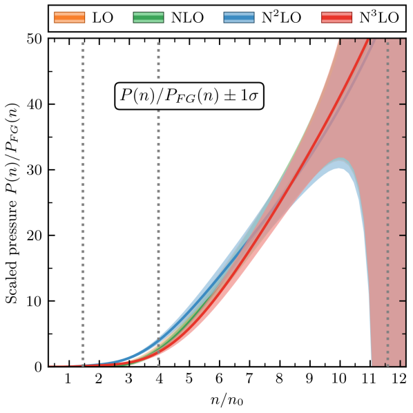
Figure 6: $\chi$EFT pressure scaled by the Fermi gas pressure and extended in the density past the highest density computed in Ref. Drischler et al. (2019); Leonhardt et al. (2020), $n\approx 2n_{0}$, using the PAL EOS (III.1), which we use here up to $100n_{0}$ (not shown). The dotted vertical lines indicate, from left to right, the densities at which the EFT expansion parameter (8) is Q={0.5, 0.7, 1.0}, respectively. Results at lower EFT orders are obscured by those at higher orders in this figure, but we only employ the full result at N³LO and hence focus here on that curve.

We also need to continue the pQCD error model down to densities $\approx n_{0}$, where QCD is no longer perturbative, in order to implement pointwise mixing. While our pQCD error bands can be formally calculated down to the density where $\alpha_{s}$ diverges—something that actually only occurs at $n<n_{0}$ for our canonical choice $X=1$—they do not account for non-perturbative effects such as renormalons Beneke (1999); Kronfeld (2024) and pairing Kurkela et al. (2024). These are expected to significantly affect QCD thermodynamics for densities below $20n_{0}$. There is therefore a significant domain in density for which the outcome of pointwise mixing depends on extrapolations of $\chi$EFT and of pQCD uncertainties that likely extrapolate the formulae outside their region of validity.

III.2 Implementation and results

We apply our pointwise Bayesian model mixing formalism that combines the two Gaussian distributions for pQCD and $\chi$EFT to the quantity $P(n)/P_{FG}(n)$. This quantity allows for a smoother crossover when model mixing—it eliminates the massive difference in scale between the $\chi$EFT and pQCD pressures. Our results are shown in Fig. 7. In Fig. 7(a), we plot the scaled pressure, $P(n)/P_{FG}(n)$, in red, blue, and purple with $1\sigma$ uncertainties for $\chi$EFT, pQCD, and the mixed model, respectively. The mixed model follows the $\chi$EFT result until approximately $2n_{0}$, where the theory begins to break down and the truncation error from missing higher-order contributions grows rapidly with density. At this point, because this is a precision-weighted theory at each point in $n$, a mixture of both $\chi$EFT and pQCD is favoured, since the uncertainties of both theories are similar in size. However, past $(3-4)n_{0}$, the uncertainty band of the pQCD EOS decreases to a smaller width than that of $\chi$EFT, and the mixed model begins to more heavily favour pQCD until, at approximately $5n_{0}$, pQCD entirely dominates the mixed model. This result is aligned with our expectations from the individual theories in regards to the size of their uncertainty bands. Also plotted in Fig. 7(a) are the experimental constraints from heavy-ion collision (HIC) data Danielewicz et al. (2002), and the theoretical result from FRG EOS Leonhardt et al. (2020), both of which are other information that we have not included in our mixing. The mixed model does not pass through the FRG contour at all, but does fall within the HIC contour until $\approx 3n_{0}$.

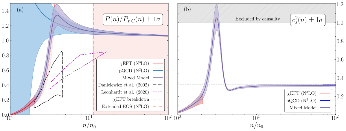
Figure 7: (a) Mixed model results from combining the extended EOS from $\chi$EFT and PAL (III.1) with pQCD results for scaled pressure $P(n)/P_{FG}(n)$ using the pointwise model mixing method (Sec. III). Here we use the expansion parameter $Q(\bar{\Lambda})=N_{f}\alpha_{s}(\bar{\Lambda})/\pi$. We overlay the results we obtain (purple band) with those of heavy-ion collision data in symmetric nuclear matter (black dash-dot contour) Danielewicz et al. (2002), and results from the functional renormalization group EOS (FRG) (pink dashed contour) Leonhardt et al. (2020). We note that the large light red region of the plot (at $n\gtrsim 10n_{0}$) corresponds to the truncation error of the extended EOS past the point where $Q=1$. Because of the sharp increase in the EOS in that density region, the mean curve is no longer visible on the plot, only this portion of the truncation error. (b) The speed of sound squared, $c_{s}^{2}(n)$, for each model. We achieve a mixed, acausal EOS with a sharp peak in the sound speed squared in the region of approximately 2-5$n_{0}$, and a result that approaches the conformal limit of 1/3 (grey dashed line) from below in the pQCD density region.

Figure 7(b) shows our result for the speed of sound squared, $c_{s}^{2}(n)$, calculated for $\chi$EFT, pQCD, and the mixed model. This was done by first integrating the pressure $P(n)$ to obtain the energy density, $\varepsilon(n)$,

$$\varepsilon(n)=n\left(\frac{\varepsilon(n_{i})}{n_{i}}+\int_{n_{i}}^{n}\frac{P(n^{\prime})}{n^{\prime 2}}dn^{\prime}\right),$$ (29)

where $\varepsilon(n_{i})$ is the value of the energy density at a particular point $n_{i}$ in the density space—in this approach, it is the initial density in $\chi$EFT where we begin our mixing, $0.05\,\text{fm}^{-3}$. We then use the thermodynamic identity

$$\mu(n)=\frac{\varepsilon(n)+P(n)}{n},$$ (30)

and obtain the speed of sound using

$$c_{s}^{2}(n)=\frac{1}{\mu}\frac{\partial P}{\partial n}.$$ (31)

The result of Eq. (31) follows that of $\chi$EFT until just under $2n_{0}$, or about where the mixed model begins to be influenced by the pQCD pressure curve (see Fig. 7(a)). The mixed model speed of sound then spikes at $\approx(3-4)n_{0}$, where the pressure curve begins to be dominated by the pQCD EOS. After this point in density, the speed of sound falls back down to below the conformal limit of 1/3, and steadily approaches this limit from below until the end of our calculation at $100n_{0}$. This behaviour is anticipated in this density region from our calculation of the sound speed squared from the pQCD EOS alone at N²LO (see Fig. 5), which is also shown in Fig. 7(b) from $70n_{0}$ onward. The mixed model result is within appropriate error bars of the individual theories, but becomes superluminal at $(3-4)n_{0}$, a result of the rapidly increasing mixed $P(n)/P_{FG}(n)$ curve.

As discussed above, a negative consequence of using this pointwise mixing approach is that information on the correlation structure in each model is discarded: we only use the variances of each model at each individual point. This also means that pointwise mixing produces only a diagonal covariance matrix for the mixed model. The mean function happens to be smooth because the data it is fit to is smooth, but this is not guaranteed with this formalism because our prior does not induce any smoothness properties across points. Furthermore, we cannot sample from a probability distribution for curves in the mixed model, because we only have a point-by-point probabilistic representation of it.

In Ref. Semposki et al. (2022), some of us argued that a prior stating the true function is smooth in the region between the two limiting theories can be included in the analysis by adding a Gaussian process to the mixed model. However, the formalism laid out above, and used in Ref. Semposki et al. (2022), assumes the models being used for the multivariate model mixing are independent, i.e., uncorrelated. This is in fact not the case for the GP constructed in Ref. Semposki et al. (2022), since it was conditioned on training data from the two models describing the low-density and high-density regions of the input space. A GP trained in this way is at least locally correlated with the models it is trained on. It is therefore a mistake to mix it with the other two models in a way that does not account for those correlations. Failing to do so effectively double counts information from the region(s) where the GP is trained.

In the next section, we discuss a conceptually simpler way to include the prior of a smooth connection between the two models in the analysis. The resulting approach also does not double count information from the input models, and makes use of their full covariance matrices, allowing us to take into account the intra-model correlation structure.

IV Correlated multivariate model mixing

In this section, we discuss the more general case of correlated Bayesian model mixing, describing how it differs from the formalism of the previous section in Sec. IV.1, and then proceeding to our implementation and results in Sec. IV.2.

IV.1 Formalism

The representation of the models adopted in the last section, in which their mean and variance are only used locally at each location in the input space $x$, underreports $\chi$EFT’s and pQCD’s relation to the underlying theory. In this section, we take advantage of the fact we have GP representations for each of the theories that are input to our BMM. We combine the information that the two multivariate Gaussians contain on the (assumed) common mean function $F(x)$ of both theories via a derivation analogous to the one in Subsec. III.1 that produced the formulae (27) for “pointwise” mixing Phillips et al. (2021). This time, however, the correlation structure of the GPs representing our input theories propagates information across the input space. The model mixing is thus “non-local” or “curvewise” once we incorporate the full information regarding the theories’ uncertainties. A benefit of such a treatment is that the non-local character of the mixing makes it unnecessary to have calculations from both input theories at every point of interest in the input space. We will show that a small number of points can be used to represent each theory, and these can be chosen in the region where the theory is reliable, with the information from that region propagating across the input space through the GP kernel(s).

We formalize this approach by adopting a GP representation for each theory that holds within that theory’s domain of validity. Just as in Sec. III.1, the pQCD and $\chi$EFT results are expressed as

$$Y^{(i)}(x)=F(x)+\delta Y^{(i)}(x),\qquad i\in[1,M],$$ (32)

where $Y^{(i)}(x)$ are each theory’s predictions and $\delta Y^{(i)}(x)$ its truncation errors. In this section the latter are assumed to take the form

$$\delta Y^{(i)}(x)\sim\textrm{GP}[0,\kappa_{y}^{(i)}(x,x^{\prime})],$$ (33)

where $\kappa_{y}^{(i)}(x,x^{\prime})$ is the covariance function that defines theory $i$’s correlations between locations $x$ and $x^{\prime}$ in the input space. Notice that Eq. (32) is exactly Eq. (20), but now we have a more sophisticated statistical model for the error structure.

Equations (33) and (32) define probability density functions (pdfs) for each theory $Y^{(i)}(x)$ that are input to the model mixing: $\operatorname{pr}(y^{(i)}(x)\,|\,f(x),\kappa_{y}^{(i)})$. We will use Bayes’ theorem to combine the information in these pdfs and infer their common mean function $F$. This requires a prior on the underlying theory, and we also adopt a GP for that:

$$F(x)\sim\textrm{GP}[0,\kappa_{f}(x,x^{\prime})].$$ (34)

In keeping with the GP flavor of these equations, we define a set of training and evaluation data. The training points should be taken to be locations where the input models, and their intra-model UQ, are reliable. The full training data set $\vec{x}_{t}$ is the concatenation of the individual training data points $\vec{x}_{t,i}$; $i=1,\ldots,M$. In our case, no duplicate entries exist in this vector, since the domains of validity of the input theories are disjoint. We also form the vector $\vec{y}=y(\vec{x}_{t})$ of data in our training space in an analogous manner, i.e., as the concatenation of $y^{(i)}(\vec{x}_{t,i})$; $i=1,\ldots,M$.

Meanwhile, we construct a multi-model theory uncertainty covariance matrix

$$K_{y}=\kappa_{y}^{(1)}(\vec{x}_{t,1},\vec{x}_{t,1}) \otimes\kappa_{y}^{(2)}(\vec{x}_{t,2},\vec{x}_{t,2})\otimes\ldots$$

$$\otimes\kappa_{y}^{(M)}(\vec{x}_{t,M},\vec{x}_{t,M})$$ (35)

that has $M$ block diagonal pieces, each of which contains an individual model’s truncation error matrix, evaluated at the training points appropriate to that model. Including correlations between the input models is formally a straightforward extension of the assumption that $K_{y}$ is block diagonal, but here we assume the $M$ models being mixed are independent. However, this does not affect the general formalism, since none of the equations below are dependent on this fact.

The evaluation points are then the locations where we want the mixed-model prediction. We combine the training and evaluation points into a single vector $\vec{x}=\{\vec{x}_{e},\vec{x}_{t}\}$, and denote the mixed-model predictions at these locations as $\vec{f}=\{\vec{f}_{e},\vec{f}_{t}\}$. We will carry out the Bayesian inference on the full vector $\vec{f}$ and then marginalize over the values $\vec{f}_{t}$ at the end of the calculation. We also take $K_{f}\equiv\kappa_{f}(\vec{x},\vec{x})$ to be the covariance matrix associated with the function prior, $\kappa_{f}$, evaluated at the full set of evaluation and training points $\vec{x}$. As we did in Sec. III, we also define a projection matrix $B_{t}$ that pulls $\vec{f}_{t}=B_{t}\vec{f}$ out of the full vector $\vec{f}$ that includes the evaluation points. The matrix $B_{e}=1-B_{t}$ selects the evaluation points from $\vec{f}$.

With these definitions in hand, we can form the log posterior of $\vec{f}$, up to constants, as

$$\log\operatorname{pr}(\vec{f}\,|\,\vec{y},K_{y},K_{f})$$

$$=-\frac{1}{2}\Bigl{[}(\vec{y}-B_{t}\vec{f}\,)^{T}K_{y}^{-1}(\vec{y}-B_{t}\vec{f}\,)+\vec{f}^{T}K_{f}^{-1}\vec{f}\,\Bigr{]}+\ldots$$

$$=-\frac{1}{2}(\vec{f}-\vec{\mu})^{T}\Sigma^{-1}(\vec{f}-\vec{\mu})+\ldots,$$ (36)

so we have shown that $\vec{f}$ is indeed distributed as a multi-variate Gaussian:

$$\vec{F}\,|\,\vec{y},K_{y},K_{f}\sim\mathcal{N}[\vec{\mu},\Sigma]$$ (37)

and the algebra that recasts the first line of Eq. (IV.1) in the form of the second line shows that

$$\vec{\mu} \equiv\Sigma B_{t}^{T}K_{y}^{-1}\vec{y},$$ (38)

$$\Sigma \equiv(K_{f}^{-1}+B_{t}^{T}K_{y}^{-1}B_{t})^{-1}.$$ (39)

The equations for the mean function $F$ differ from those for the pointwise case, Eq. (III.1), via the inclusion of a full covariance matrix for both $\kappa_{f}$ and each of the models being mixed (via $K_{y}$). The pointwise strategy presented in Sec. III.1 is thus a limiting case of the one presented here; nevertheless, it remains true that we are combining information on the common mean of a set of Gaussian random variables, so the pdf of that mean will also be a Gaussian.

We now execute the final step of the calculation, which is to focus on the evaluation points, and exclude the training information from $\mu$ and $\Sigma$. After using the Woodbury matrix identity and applying $B_{e}$ to single out the evaluation points in the above equations, we obtain

$$\vec{\mu}_{e} =K_{f,et}(K_{f,tt}+K_{y,tt})^{-1}\vec{y},$$ (40)

$$\Sigma_{ee} =K_{f,ee}-K_{f,et}(K_{f,tt}+K_{y,tt})^{-1}K_{f,te},$$ (41)

where we use the training and evaluation subscripts as before. It is no coincidence that these equations have the exact form of the conditional updating equations of a Gaussian process, i.e., Rasmussen and Williams (2006)

$$\vec{\mu}_{x_{*}} = K_{f,x_{*}x}(K_{f,xx}+K_{y,xx})^{-1}\vec{y},$$

$$\Sigma_{x_{*}x_{*}} = K_{f,x_{*}x_{*}}-K_{f,x_{*}x}$$ (42)

$$\hbox{}\times(K_{f,xx}+K_{y,xx})^{-1}K_{f,xx_{*}},$$

where $x$ are the training points, $x_{*}$ are the evaluation points, and $K_{ij}\equiv\kappa(\vec{x}_{i},\vec{x}_{j})$.

We have derived the GP conditional updating formulae from our initial Bayesian analysis. It follows that we have obtained a GP representation of the mixed model $F$. That GP is formed from the covariance structure of the input models, evaluated at the training points, and the prior on $F$. These covariance matrices together determine how the models should be mixed.

IV.2 Implementation and results

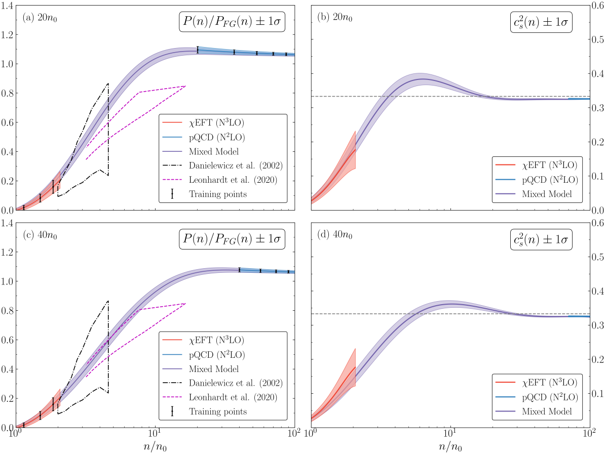
Figure 8: (a), (c): Mixed model results from combining $\chi$EFT and pQCD results for scaled pressure $P(n)/P_{FG}(n)$ using the correlated model mixing approach (Sec. IV) via a Gaussian process. Here we implement pQCD training cutoffs of $20n_{0}$ and $40n_{0}$, respectively. We overlay the results we obtain (purple band) with those of heavy-ion collision data in symmetric nuclear matter (black dash-dot contour) Danielewicz et al. (2002), and results from the functional renormalization group (FRG) (pink dashed contour) Leonhardt et al. (2020). We note the remarkable agreement between the mixed model and the HIC contour in (a) and (c), and the FRG contour around $2-4n_{0}$ in (c). (b), (d): The results for the speed of sound squared, $c_{s}^{2}(n)$, corresponding to (a) and (c), respectively. The results possess a smoother, gradual peak in the mixed model sound speed squared in the region of approximately $10n_{0}$ compared to Fig. 7, and approach the conformal limit of 1/3 (grey dashed line) from below in the pQCD density region, like the accepted pQCD result shown in Fig. 5.

To apply the formalism of the previous subsection, we must choose the prior on the underlying theory $\kappa_{f}(x,x^{\prime})$. Here, we adopt the Radial Basis Function (RBF) kernel with a marginal variance $\bar{c}^{2}$. This choice of prior for the function space of $F$ carries with it several assumptions. First, $F$ is assumed to be infinitely differentiable: phase transitions are precluded by this aspect of the prior. Second, this is a stationary kernel. An important technical point is that the GP is formulated in $\ln({n})$ space, rather than in the density $n$ itself. This is essential if pQCD is to be described by a stationary GP, since $\alpha_{s}$ runs logarithmically. Nevertheless, the assumption of stationarity means that we are implicitly assuming there is persistence in both the size and lengthscale of the variability in the dense matter EOS, i.e., the broad pattern of variations in the EOS that occurs in the pQCD and $\chi$EFT domains persists throughout the complete range of density. Neither of these assumptions have to be satisfied by QCD. Testing their validity is an important topic for future investigations. But, as usual, Bayesian methods provide a clear way to delineate the consequences of such assumptions for the quantity of interest, i.e., the dense matter EOS.

We reiterate that because the GP for $F$ can be (actually must be!) evaluated away from its training points, we do not need $\chi$EFT and pQCD to be evaluated at all the points in density for which we wish to know the mixed model result, as was necessary in Sec. III.1. We use, in fact, a fairly small training set of four to five points that are clearly in the pQCD domain ($n\geq 20n_{0}$) and four points that are clearly in the $\chi$EFT domain ($n\leq 2n_{0}$). The training data is listed in Table 2. At least three training points below $2n_{0}$ are needed in order to describe $\chi$EFT well; we also verified that adding more pQCD training points within the range $40n_{0}<n<100n_{0}$ does not change the result.

We know that nonperturbative effects, not accounted for in the pQCD truncation-error model, will eventually significantly alter the pQCD EOS as we move to lower and lower densities. But, we do not know where these effects reach a magnitude large enough to invalidate our truncation-error model. Because of this, we choose to adopt two “priors” regarding the validity of errors derived from pQCD convergence. We train on pQCD predictions (1) $\geq 20n_{0}$ and (2) $\geq 40n_{0}$. We then investigate the sensitivity of the resulting mixed model to this cutoff.

We implement the GP for $F$ using a modified version of the scikit-learn Python package Pedregosa et al. (2011). To train on the data set we have chosen, we create a total covariance matrix out of the two models’ respective covariance matrices, such that the resulting matrix input to the GP is block diagonal in model space. We then fit to the training data in Table 2 in $\ln(n)$ space and predict at a dense grid across the density space, up to $100n_{0}$. Figure 8 shows the results from training on $\chi$EFT and pQCD in the two different scenarios outlined previously. The lengthscales that we found to produce the maximum likelihood for each of our training data sets are: (1) $\ell=1.46$ and (2) $\ell=1.86$ (all in $\ln(n)$). The corresponding marginal variances are (1) $\bar{c}^{2}=0.648$ and (2) $\bar{c}^{2}=0.603$.

Table 2: The set of training data taken from $\chi$EFT (N³LO) and pQCD (N²LO) to train the correlated mixing GP. Here we list the location in the scaled density $n/n_{0}$, and the mean and variance at each point. We report values for the two cutoffs used in the pQCD results of this section. We note that though we have only included the variances in the table, we use the full covariance matrices for these points in our training procedure.

	$n/n_{0}$	$P(n)/P_{FG}(n)$	$\sigma_{y}(n)$
	$0.78$	$-0.0257$	$0.007$
$\chi$EFT	$1.14$	$0.0171$	$0.015$
	$1.49$	$0.0830$	$0.028$
	$1.85$	$0.160$	$0.045$
	$20.11$	$1.095$	$0.023$
pQCD	$36.75$	$1.08$	$0.015$
$(20n_{0})$	$53.40$	$1.073$	$0.012$
	$70.04$	$1.068$	$0.010$
	$86.69$	$1.065$	$0.009$
	$40.08$	$1.078$	$0.014$
pQCD	$56.73$	$1.072$	$0.012$
$(40n_{0})$	$73.37$	$1.068$	$0.010$
	$90.01$	$1.065$	$0.009$

The mixed model for $P(n)/P_{FG}(n)$ is in very good agreement with the EOS constraints from HIC data Danielewicz et al. (2002) for both EOSs (1) and (2) (i.e. both sets of pQCD training data). It falls within the FRG EOS constraint Leonhardt et al. (2020) in the case where we take training data only at $n\geq 40n_{0}$. Unsurprisingly, given the kernel choice adopted for $\kappa_{f}$ here, the mixed model predicts a smooth crossover from $\chi$EFT to pQCD in both cases.

To provide easy access to our results, in Table 3, we provide the mean and standard deviation of the $P(n)$ distribution in our mixed-model EOS at densities of $4n_{0}$, $12n_{0}$, and $36n_{0}$. We list values for the EOS trained on both pQCD training cutoffs ($\geq 20n_{0}$ and $\geq 40n_{0}$). For comparison, we also provide the pQCD $P(n)$, and its uncertainty, at these same densities for our canonical choice of $X=1$. Full results will be found in the open-source GitHub repository that will accompany this work.

To obtain the speed of sound, we sample the GP scaled $P(n)/P_{FG}(n)$ curve and use the procedure described in Eqs. (29)-(31) to calculate $c_{s}^{2}(n)$ for each curve. We set $\varepsilon(n_{i})$ to the value of the energy density at $n_{i}=100n_{0}$ in the pQCD EOS, as this yields a stable result when integrating downward to lower densities to obtain $\varepsilon(n)$. The undramatic nature of the transition from $\chi$EFT to pQCD is reflected in our results for the speed of sound shown in Fig. 8(b) and (d). Both cases exhibit a speed of sound that peaks much more gradually than in the pointwise mixing results of Sec. III.2. Training the mixed model with data from lower densities in pQCD [case (1)] does result in a more peaked speed of sound in comparison with training only at $n\geq 40n_{0}$ [case (2)]. This is related to the GP’s tendency to smoothly join the $\chi$EFT and pQCD curves. Nevertheless, each curve does approach the conformal limit $c_{s}^{2}=1/3$ from below in the region where pQCD is valid, also as expected given the pQCD results of Appendix B for the consistent $c_{s}^{2}$ calculation to $\mathcal{O}(\alpha_{s}^{2})$.

Table 3: A set of single values of each EOS. As in the main text, $\chi$EFT is taken at N³LO, and pQCD at N²LO. The mixed model is the correlated Bayesian model mixing result from the GP implementation in Sec. IV.2, calculated using each chosen cutoff in pQCD ($20n_{0}$ and $40n_{0}$, respectively). The chemical potential is computed using the perturbative expansion in the KLW formalism. Higher-precision, machine-readable data will be found in our GitHub repository.

		$P(n)$ [MeV/fm3]
$n/n_{0}$	$\mu_{q}$ [GeV]	pQCD	GP
		$X=1$	Case (1)	Case (2)
4	0.554	253.8 (30.7)	131.1 (9.7)	108.1 (9.1)
12	0.696	1000.1 (31.9)	954.0 (27.4)	876.1 (25.3)
36	0.958	4188.9 (59.3)	4164.5 (58.0)	4173.1 (58.3)

We note the slight difference between the error bars of the GP mixed model result and those of the individual theories in their respective regions, seen most clearly in $P(n)/P_{FG}(n)$ at $\approx 2n_{0}$ in Fig. 8. This is primarily caused by the combination of Gaussian random variables in both approaches (Secs. III.1 and IV.1), which leads to smaller error bars of the mixed results. This is a consequence of our assumption of a common mean for the two input theories. A reduction of uncertainty always occurs when a common mean is inferred from two (or more) independent random variables.

V Summary and outlook

Recent developments have yielded representations of the equation of state (EOS) of dense QCD matter in the two complementary regimes of ultra-high density and densities up to two times nuclear saturation density as Gaussian probability distributions. Both calculations—the former from perturbative QCD (pQCD) and the latter from chiral effective field theory ($\chi$EFT)—come with correlated theory uncertainties across densities and are derived from the order-by-order convergence pattern of the perturbative series. In this work, we demonstrated two ways by which these two (presumably independent) Gaussian random variables can be used to infer what we take to be a common mean, so producing a unified equation of state for QCD matter, with quantified uncertainties, for densities all the way from nuclear saturation to asymptotically free quarks. Our proof-of-principle calculations carried out this Bayesian model mixing for symmetric, two-flavor strongly interacting matter.

The theory input to the mixing was:

• The $\chi$EFT pressure at N³LO as a function of number density, including a correlated EFT uncertainty in the density $n$, as computed in Refs. Drischler et al. (2019, 2020b, 2020a).

• The N²LO pQCD pressure as a function of $n$. We convert the N²LO results of Ref. Gorda et al. (2023a) for $P(\mu)$ to $P(n)$ in a way that strictly preserves the perturbative expansion of $P$ using the method of Kohn, Luttinger, and Ward Kohn and Luttinger (1960); Luttinger and Ward (1960). We applied the BUQEYE truncation error model of Melendez et al. (2019) to the pQCD EOS to compute the covariance structure associated with N³LO-and-beyond uncertainties in the EOS.

We first combined the two Gaussian probability distributions thereby obtained via the pointwise mixing method of Ref. Semposki et al. (2022). This approach replaces the full covariance matrix of each theory by its diagonal element at each density and then precision weights the two theories to obtain the underlying mean. However, since there is no density where both $\chi$EFT and pQCD converge such pointwise combination of theories necessitates uncontrolled extrapolation of the central value of $\chi$EFT and both theories’ error bands into regions where the theories break down.

The second approach to combined inference demonstrated here uses the full Gaussian structure of both theories’ probability distributions to obtain a Gaussian process (GP) representation for the underlying theory on which both calculations are based. In this case, non-local propagation of information from the $\chi$EFT and pQCD calculations avoids the need to extrapolate either beyond their domain of validity. The details of that propagation are controlled by the prior on the function space in which the curve-wise mixing takes place, i.e., the choice of GP kernel. For the first work on this topic, we adopted the popular radial basis-function (RBF, aka “squared exponential”) kernel. The $P(n)$ probability distribution this produces for pQCD training data at $n\geq 40n_{0}$ is consistent with constraints from a Functional Renormalization Group (FRG) calculation Leonhardt et al. (2020). The distributions from both pQCD training-data cutoffs are consistent with inference from Heavy-Ion Collisions (HIC) Danielewicz et al. (2002). The corresponding speed of sound, $c_{s}^{2}(n)$, is tightly constrained, although whether, and by how much, $c_{s}^{2}$ exceeds $1/3$ at $n\approx 10$ times saturation density depends on the lowest density at which pQCD central values and uncertainties for $P(n)$ are trustworthy.

Irrespective of the minimum density at which pQCD input is employed, our result for $c_{s}^{2}(n)$ approaches $1/3$ smoothly from below as $n$ becomes larger than 40 times the saturation density. This is consistent with the result derived in Appendix B that the pQCD speed of sound is 1/3 with a calculable correction of $\mathcal{O}(\alpha_{s}^{2})$ whose coefficient is negative because of asymptotic freedom.

The results produced here could be refined by replacing the N²LO pQCD $P(n)$ by the almost-complete N³LO calculation of Ref. Gorda et al. (2023a). Nonzero quark masses Kurkela et al. (2010); Fraga and Romatschke (2005), can also be incorporated in the pQCD calculation. We note, however, that the accuracy of our calculation is not limited by the pQCD input used here, since the error bands we derived for the pQCD $P(n)$ remain narrow down to densities well below those at which non-perturbative effects (e.g., renormalon ambiguities Beneke (1999); Kronfeld (2024) or pairing Kurkela et al. (2024)) are expected to markedly affect the pressure. QCD calculations that have reliably quantified uncertainties at intermediate densities where non-perturbative effects play a significant role would be very valuable; rigorous uncertainty quantification for the FRG results Leonhardt et al. (2020) would be a big step forward in this regard. Any non-perturbative QCD calculation of this character could be straightforwardly added to our multi-model Bayesian inference.

The impact that different choices for the GP kernel have on the correlated mixing is an important topic for further study. The RBF kernel imposes strong assumptions in regard to the smoothness of the curves representing the underlying theory. This can drive the resulting trained GP towards overly narrow probability distributions (see, e.g., Ref. Semposki et al. (2022)). It precludes phase transitions and other interesting structures of the types discussed in Ref. Mroczek et al. (2023). Relaxing the kernel so that the underlying function can have less differentiability, or even be non-differentiable, is an ongoing investigation. Composite kernels, such as changepoint kernels Garnett et al. (2010), are also promising options. The results obtained in the model-mixed EOS with different GP kernels can then be validated using HIC data, which has recently been used for EOS inference Huth et al. (2022); Yao et al. (2023); Komoltsev et al. (2023), or from neutron star observations. This validation would benefit from FRIB400 FRIB Science Community (2021); Nuclear Science Advisory Committee (2023) (NSAC), the proposed 400 MeV/u (uranium) energy upgrade of the Facility for Rare Isotope Beams (FRIB) at Michigan State University, which would provide new experimental constraints on dense matter up to twice the saturation density.

However, the matter described in this work is not neutron-rich matter; extending this study to the case of asymmetric nuclear matter Drischler et al. (2021b); Kurkela et al. (2010); Gorda et al. (2018, 2021b, 2021a) and specifically beta-equilibrated, charge-neutral matter (i.e., neutron star matter) Lattimer and Prakash (2001, 2004); Lattimer (2021) is a straightforward and important future task. This extension would also provide the opportunity to incorporate the stability constraints discussed in Refs. Komoltsev and Kurkela (2022); Komoltsev et al. (2023). The resulting EOSs could be validated against neutron star observations, including NICER and XMM-Newton data (see, e.g., Refs. Miller et al. (2021); Riley et al. (2021); Salmi et al. (2022); Vinciguerra et al. (2024)), and provide insights into the structure of and maximum sound speed in neutron stars (see, e.g., Refs. Drischler et al. (2021b, 2022)). Ultimately, it is also important to extend our methods to mixing across the two-dimensional input space of density and temperature, so providing a unified EOS with quantified uncertainties for numerical simulations of neutron star mergers Radice et al. (2018).

The inference techniques applied in this paper are in no way specific to $P(n)$ for symmetric two-flavor matter; it applies in any situation where there is a common mean that has been estimated in two independent ways Bates and Granger (1969). This work establishes the feasibility and usefulness of this way of combining random variables for dense-matter equations of state, and will provide open-source software to facilitate broad applications of the presented BMM framework.

Appendix A Converting pQCD from P($\mu$) to P(n)

This approach follows the work of Kohn, Luttinger, and Ward Kohn and Luttinger (1960); Luttinger and Ward (1960), detailed, e.g., in Ref. Fetter and Walecka (1972). First, we define the pressure of perturbative QCD in the manner of Eq. (1), where we choose the expansion parameter $Q(\bar{\Lambda})=N_{f}\alpha_{s}(\bar{\Lambda})/\pi$, and the number density as the derivative of the pressure with respect to the quark chemical potential $\mu$, such that

$$P(\mu) = P_{FG}(\mu)\bigg{[}c_{0}+c_{1}Q(\bar{\Lambda})+c_{2}(\mu)Q^{2}(\bar{\Lambda})\bigg{]},$$

$$n(\mu) = \frac{\partial P(\mu)}{\partial\mu},$$ (43)

where

$$c_{0} = 1,\qquad c_{1}=\frac{a_{1,1}}{N_{f}},$$

$$c_{2}(\mu) = \frac{1}{N_{f}}\bigg{(}a_{2,1}\ln{\left(\frac{N_{f}\alpha_{s}(\bar{\Lambda})}{\pi}\right)}$$ (44)

$$+ a_{2,2}\ln{\left(\frac{\bar{\Lambda}}{2\mu}\right)}+a_{2,3}\bigg{)}.$$

Note that the expansion parameter could be chosen differently, and this formalism can easily be altered to incorporate this, with the coefficients altered to account for the difference.

We then define the perturbative expansion of the quark chemical potential as

$$\mu=\mu_{FG}+\mu_{1}+\mu_{2},$$ (45)

which we only take up to second order due to only having terms in $P(\mu)$ to this order. We expand the number density of Eq. (A) about the point $\mu=\mu_{FG}$, and set

$$n_{FG}(\mu)=c_{0}\frac{\partial P_{FG}(\mu)}{\partial\mu}\bigg{|}_{\mu=\mu_{FG}}.$$ (46)

The number density at the Fermi gas (FG) chemical potential, $n(\mu_{FG})$, is obtained from the first term in this series, and each piece of $\mu$ beyond leading order (LO) is arranged such that the leading order result is unchanged at a specific order in $\alpha_{s}$. Keeping only the terms up to $\alpha_{s}$ and $\alpha_{s}^{2}$, respectively, we thus obtain results for $\mu_{1}$ and $\mu_{2}$

$$\mu_{1} = -\frac{c_{1}Q(\bar{\Lambda})\frac{\partial P_{FG}(\mu)}{\partial\mu}}{c_{0}\frac{\partial^{2}P_{FG}(\mu)}{\partial\mu^{2}}}\Bigg{|}_{\mu=\mu_{FG}},$$ (47)

$$\mu_{2} = -\frac{1}{c_{0}\frac{\partial^{2}P_{FG}(\mu)}{\partial\mu^{2}}}\bigg{[}\frac{\mu_{1}^{2}}{2}c_{0}\frac{\partial^{3}P_{FG}(\mu)}{\partial\mu^{3}}$$ (48)

$$+ \mu_{1}c_{1}Q(\bar{\Lambda})\frac{\partial^{2}P_{FG}(\mu)}{\partial\mu^{2}}$$

$$+ c_{1}\frac{\partial Q(\bar{\Lambda})}{\partial\mu}P_{FG}(\mu)$$

$$+ \frac{\partial c_{2}(\mu)}{\partial\mu}Q^{2}(\bar{\Lambda})P_{FG}(\mu)$$

$$+ c_{2}(\mu)Q^{2}(\bar{\Lambda})\frac{\partial P_{FG}(\mu)}{\partial\mu}\bigg{]}\Bigg{|}_{\mu=\mu_{FG}}.$$

Now we can recast $\mu_{1}$ and $\mu_{2}$ into expressions containing the number density $n_{FG}(\mu_{FG})$ and simplify to get

$$\mu_{1} = -\frac{c_{1}Q(\bar{\Lambda}_{FG})\mu_{FG}}{3c_{0}},$$

$$\mu_{2} = \frac{2c_{1}^{2}}{9c_{0}^{2}}\mu_{FG}Q^{2}(\bar{\Lambda}_{FG})-\frac{\mu_{FG}}{3c_{0}}c_{2}(\mu_{FG})Q^{2}(\bar{\Lambda}_{FG})$$ (49)

$$- \frac{\mu_{FG}^{2}}{12c_{0}}\frac{\partial c_{2}(\mu)}{\partial\mu}Q^{2}(\bar{\Lambda}_{FG})\Bigg{|}_{\mu=\mu_{FG}}$$

$$- \frac{c_{1}}{12c_{0}}\mu_{FG}^{2}\frac{\partial Q(\bar{\Lambda})}{\partial\mu}\Bigg{|}_{\mu=\mu_{FG}}.$$

We note that $\bar{\Lambda}_{FG}\equiv\bar{\Lambda}(\mu_{FG})\equiv 2X\mu_{FG}$, and $\frac{\partial Q(\bar{\Lambda})}{\partial\mu}$ can be analytically determined at the one-loop level to be Vermaseren et al. (1997)

$$\frac{\partial Q(\bar{\Lambda})}{\partial\mu}\equiv\frac{N_{f}}{\pi}\frac{\partial\alpha_{s}(\bar{\Lambda})}{\partial\mu}=-N_{f}\frac{\beta_{0}}{\mu}\frac{\alpha_{s}^{2}(\bar{\Lambda})}{2\pi^{2}}.$$ (50)

We can also define

$$\frac{\partial c_{2}(\mu)}{\partial\mu}=-\frac{1}{N_{f}}\frac{a_{2,1}}{\alpha_{s}(\bar{\Lambda})}\frac{\partial\alpha_{s}(\bar{\Lambda})}{\partial\mu};$$ (51)

however, this term is of $\mathcal{O}(\alpha_{s})$, hence inserting for this term in Eq. (A) leads to an expression of $\mathcal{O}(\alpha_{s}^{3})$, so we hereafter drop this term from $\mu_{2}$.

We can then expand the pressure in a Taylor series about $\mu=\mu_{FG}$ and keep terms to second order in $\alpha_{s}$, again, to obtain

$$P(\mu) \simeq c_{0}P_{FG}(\mu_{FG})$$ (52)

$$+ (\mu_{1}+\mu_{2})c_{0}\frac{\partial P_{FG}(\mu)}{\partial\mu}\Bigg{|}_{\mu=\mu_{FG}}$$

$$+ c_{1}Q(\bar{\Lambda}_{FG})P_{FG}(\mu_{FG})$$

$$+ \frac{\mu_{1}^{2}}{2}c_{0}\frac{\partial^{2}P_{FG}(\mu)}{\partial\mu^{2}}\Bigg{|}_{\mu=\mu_{FG}}$$

$$+ \mu_{1}c_{1}Q(\bar{\Lambda}_{FG})\frac{\partial P_{FG}(\mu)}{\partial\mu}\Bigg{|}_{\mu=\mu_{FG}}$$

$$+ c_{2}(\mu_{FG})Q^{2}(\bar{\Lambda}_{FG})P_{FG}(\mu_{FG}).$$

Organising this in terms of powers of $\alpha_{s}$ and inserting $\mu_{1}$ and $\mu_{2}$, and dividing by the FG pressure $P_{FG}(\mu_{FG}(n))$, we can express the scaled pressure with respect to number density $n$ as

$$\frac{P(n)}{P_{FG}(n)} = c_{0}-\frac{1}{3}c_{1}Q(\bar{\Lambda}_{FG})$$ (53)

$$+ \frac{2}{9}\frac{c_{1}^{2}}{c_{0}}Q^{2}(\bar{\Lambda}_{FG})-\frac{1}{3}c_{2}(\mu_{FG})Q^{2}(\bar{\Lambda}_{FG})$$

$$- \frac{\mu_{FG}}{3}c_{1}\frac{\partial Q(\bar{\Lambda})}{\partial\mu}\Bigg{|}_{\mu=\mu_{FG}},$$

Now we insert the coefficients from Eq. (A) and the expansion parameter as previously mentioned to obtain

$$\frac{P(n)}{P_{FG}(n)} = 1+\frac{2}{3\pi}\alpha_{s}(\bar{\Lambda}_{FG})$$ (54)

$$+ \frac{8}{9\pi^{2}}\alpha_{s}^{2}(\bar{\Lambda}_{FG})-\frac{N_{f}^{2}}{3\pi^{2}}c_{2}(\mu_{FG})\alpha_{s}^{2}(\bar{\Lambda}_{FG})$$

$$- \frac{\beta_{0}}{3\pi^{2}}\alpha_{s}^{2}(\bar{\Lambda}_{FG}),$$

which is equivalent to Eq. (16). The first line of this equation contains the LO and NLO terms of the series, and the following lines contain all N²LO terms. We have now expressed the pressure in terms of number density, while keeping consistent truncation at second order in the number density and the pressure. Note that this consistent KLW inversion leads to NLO and N²LO coefficients in the pQCD expansion of $P(n)$ that are both smaller, by factors of precisely and roughly $1/3$ respectively, than the coefficients in $P(\mu)$.

Appendix B Order-by-order speed of sound: P($\mu$) and P($n$)

B.1 Calculating P($\mu$)

We can first define, from QCD, the renormalization group (RG) equation for the running coupling Zyla et al. (2020),

$$\bar{\Lambda}^{2}\frac{d\alpha_{s}(\bar{\Lambda})}{d\bar{\Lambda}^{2}}=-(b_{0}\alpha_{s}^{2}+b_{1}\alpha_{s}^{3}+\dots),$$ (55)

where $b_{0}=\beta_{0}/4\pi$ and $b_{1}=2\beta_{1}/(4\pi)^{2}$. In this calculation, we will only need to use the one-loop beta function to maintain consistency, so we truncate Eq. (55) after $\mathcal{O}(\alpha_{s}^{2})$.

We want to obtain the speed of sound from $P(\mu)$ up to second order in $\alpha_{s}$, so we will use Eqs. (13) and (18). Taking the first derivative of Eq. (13), we obtain

$$\frac{\partial P}{\partial\mu} = P_{FG}(\mu)\frac{\partial}{\partial\mu}\left(\frac{P(\mu)}{P_{FG}(\mu)}\right)$$ (56)

$$+ n_{FG}(\mu)\left(\frac{P(\mu)}{P_{FG}(\mu)}\right).$$

Then, taking the second derivative of $P(\mu)$, we drop all powers of $\alpha_{s}^{3}$ and above, since we are only interested in the orders up to $\alpha_{s}^{3}$ to maintain thermodynamic consistency. We then series expand in $\alpha_{s}$ and obtain

$$c_{s}^{2}(\mu)\simeq\frac{1}{3}+\mathcal{O}(\alpha_{s}^{2}).$$ (57)

Hence, no terms at next-to-leading order (NLO) contribute to the sound speed squared with respect to the chemical potential for the pQCD EOS.

The coefficient of the N²LO term is computed to be

$$\frac{5}{108\pi^{2}}(-33+2N_{f})\approx-0.136033,$$ (58)

indicating an approach to the conformal limit from below at the N²LO level for symmetric matter.

It is interesting to note that, if $\alpha_{s}(\bar{\Lambda})$ were not a running coupling constant but a simple scalar, the result for the total $c_{s}^{2}(n)$ through N²LO would be 1/3. As such, the speed of sound directly probes the running of $\alpha_{s}(\bar{\Lambda})$ in pQCD.

B.2 Calculating P($n$)

Due to the relation in Eq. (19), we can prove in a few simple steps that $c_{s}^{2}(\mu)\equiv c_{s}^{2}(n)$. We do this by using the quark number density and the quark chemical potential $\mu_{q}=\mu_{FG}+\mu_{1}+\mu_{2}$ from Appendix A, which implicitly contains the number density. We can write

$$c_{s}^{2}(\mu(n))=\frac{n}{\mu}\frac{\partial\mu}{\partial n}\Bigg{|}_{n=\bar{n}}\equiv\frac{\bar{n}}{(\mu_{FG}+\mu_{1}+\mu_{2})}\frac{\partial(\mu_{FG}+\mu_{1}+\mu_{2})}{\partial n}\Bigg{|}_{n=\bar{n}}\equiv\frac{c_{s,FG}^{2}(\bar{n})}{\left(1+\frac{\mu_{1}}{\mu_{FG}}+\frac{\mu_{2}}{\mu_{FG}}\right)}\left(1+\frac{\partial\mu_{1}}{\partial\mu_{FG}}+\frac{\partial\mu_{2}}{\partial\mu_{FG}}\right),$$ (59)

where the Fermi gas sound speed squared is given by

$$c_{s,FG}^{2}(\bar{n})=\frac{\bar{n}}{\mu_{FG}}\frac{\partial\mu_{FG}}{\partial n}\Bigg{|}_{n=\bar{n}}.$$ (60)

Here, $\bar{n}$ is a given quark number density.

Taking a series expansion of the denominator in Eq. (59) and truncating any terms we know will yield $\mathcal{O}(\alpha_{s}^{3})$ or higher immediately, we obtain

$$c_{s}^{2}(\mu(n)) = c_{s,FG}^{2}(\bar{n})\Bigg{[}1-\frac{\mu_{1}}{\mu_{FG}}-\frac{\mu_{2}}{\mu_{FG}}+\frac{\mu_{1}^{2}}{\mu_{FG}^{2}}$$ (61)

$$+ \frac{\partial\mu_{1}}{\partial\mu_{FG}}-\frac{\mu_{1}}{\mu_{FG}}\left(\frac{\partial\mu_{1}}{\partial\mu_{FG}}\right)-\frac{\mu_{2}}{\mu_{FG}}$$

$$+ \left(\frac{\partial\mu_{2}}{\partial\mu_{FG}}\right)+\mathcal{O}(\alpha_{s}^{3})\Bigg{]}.$$

From Eqs. (A), we can construct the expressions for all of the terms in Eq. (61). After simplification and use of Eq. (50), these are

$$\frac{\mu_{1}}{\mu_{FG}} = \frac{2}{3\pi}\alpha_{s}(\bar{\Lambda}),$$

$$\frac{\mu_{2}}{\mu_{FG}} = \frac{8}{9\pi^{2}}\alpha_{s}^{2}(\bar{\Lambda})-\frac{4}{3\pi^{2}}c_{2}(\mu_{FG})\alpha_{s}^{2}(\bar{\Lambda})$$

$$+ \frac{\mu_{FG}}{3\pi}\alpha_{s}^{\prime}(\bar{\Lambda}),$$

$$\frac{\partial\mu_{1}}{\partial\mu_{FG}} = \frac{\mu_{1}}{\mu_{FG}}+\frac{4}{3\pi}\mu_{FG}\alpha_{s}^{\prime}(\bar{\Lambda}),$$

$$\frac{\partial\mu_{2}}{\partial\mu_{FG}} = \frac{\mu_{2}}{\mu_{FG}}+\frac{\mu_{FG}}{3\pi}\alpha_{s}^{\prime}(\bar{\Lambda}),$$ (62)

where $\alpha_{s}^{\prime}(\bar{\Lambda})=\partial\alpha_{s}(\bar{\Lambda})/\partial\bar{\Lambda}$.

Next, we insert these expressions in Eq. (61), truncate any terms above $\mathcal{O}(\alpha_{s}^{2})$, achieving the relation

$$c_{s}^{2}(\mu(n)) = c_{s,FG}^{2}(\bar{n})\left(1+\frac{5}{3\pi}\mu_{FG}\alpha_{s}^{\prime}(\bar{\Lambda})\right),$$ (63)

$$= \frac{1}{3}\left(1-\frac{5}{3\pi}\beta_{0}\alpha_{s}^{2}(\bar{\Lambda})\right),$$

where we have inserted $c_{s,FG}^{2}(\bar{n})=\frac{1}{3}$ and the derivative $\partial\alpha_{s}(\bar{\Lambda})/\partial\bar{\Lambda}=-(2/\bar{\Lambda})\alpha_{s}^{2}(\bar{\Lambda})$, which can be seen from Eq. (55). This calculation numerically yields an N²LO coefficient of

$$-\frac{5}{108\pi^{2}}(33-2N_{f})\approx-0.136033,$$ (64)

which exactly matches the result from Eq. (58), where we calculated $c_{s}^{2}(\mu)$ directly from the pQCD pressure (see Eq. 13). This argument proves that the KLW inversion yields the correct relation for both $P(n)$ and $c_{s}^{2}(n)$ up to and including N²LO, further validating our procedure in Appendix A.

References

- Vitale (2021) S. Vitale, Science 372, abc7397 (2021), arXiv:2011.03563 [gr-qc] .
- Corsi et al. (2024) A. Corsi et al., (2024), arXiv:2402.13445 [astro-ph.HE] .
- Koehn et al. (2024) H. Koehn et al., (2024), arXiv:2402.04172 [astro-ph.HE] .
- Hammer et al. (2020) H.-W. Hammer, S. König, and U. van Kolck, Rev. Mod. Phys. 92, 025004 (2020), arXiv:1906.12122 .
- Tews et al. (2020) I. Tews, Z. Davoudi, A. Ekström, J. D. Holt, and J. E. Lynn, J. Phys. G 47, 103001 (2020), arXiv:2001.03334 .
- Hergert (2020) H. Hergert, Front. in Phys. 8, 379 (2020), arXiv:2008.05061 .
- Drischler et al. (2021a) C. Drischler, J. W. Holt, and C. Wellenhofer, Annu. Rev. Nucl. Part. Sci. 71, 403 (2021a), arXiv:2101.01709 .
- Melendez et al. (2019) J. A. Melendez, R. J. Furnstahl, D. R. Phillips, M. T. Pratola, and S. Wesolowski, Phys. Rev. C 100, 044001 (2019), arXiv:1904.10581 .
- Drischler et al. (2020a) C. Drischler, J. A. Melendez, R. J. Furnstahl, and D. R. Phillips, Phys. Rev. C 102, 054315 (2020a), arXiv:2004.07805 [nucl-th] .
- Drischler et al. (2020b) C. Drischler, R. J. Furnstahl, J. A. Melendez, and D. R. Phillips, Phys. Rev. Lett. 125, 202702 (2020b), arXiv:2004.07232 [nucl-th] .
- Adhikari et al. (2021) D. Adhikari et al. (PREX), Phys. Rev. Lett. 126, 172502 (2021), arXiv:2102.10767 .
- Adhikari et al. (2022) D. Adhikari et al. (CREX), Phys. Rev. Lett. 129, 042501 (2022), arXiv:2205.11593 [nucl-ex] .
- Sorensen et al. (2024) A. Sorensen et al., Prog. Part. Nucl. Phys. 134, 104080 (2024), arXiv:2301.13253 .
- Kumar et al. (2023) R. Kumar et al. (MUSES), (2023), arXiv:2303.17021 .
- Melendez et al. (2022) J. A. Melendez, C. Drischler, R. J. Furnstahl, A. J. Garcia, and X. Zhang, J. Phys. G 49, 102001 (2022), arXiv:2203.05528 [nucl-th] .
- Drischler et al. (2023) C. Drischler, J. A. Melendez, R. J. Furnstahl, A. J. Garcia, and X. Zhang, Front. Phys. 10, 92931 (2023), supplemental, interactive Python code can be found on the companion website https://github.com/buqeye/frontiers-emulator-review, arXiv:2212.04912 .
- Jiang et al. (2022) W. G. Jiang, C. Forssén, T. Djärv, and G. Hagen, (2022), arXiv:2212.13216 [nucl-th] .
- Duguet et al. (2023) T. Duguet, A. Ekström, R. J. Furnstahl, S. König, and D. Lee, (2023), arXiv:2310.19419 [nucl-th] .
- Gorda et al. (2023a) T. Gorda, R. Paatelainen, S. Säppi, and K. Seppänen, Phys. Rev. Lett. 131, 181902 (2023a), arXiv:2307.08734 [hep-ph] .
- Gorda et al. (2023b) T. Gorda, O. Komoltsev, and A. Kurkela, Astrophys. J. 950, 107 (2023b), arXiv:2204.11877 [nucl-th] .
- Gorda et al. (2021a) T. Gorda, A. Kurkela, R. Paatelainen, S. Säppi, and A. Vuorinen, Phys. Rev. D 104, 074015 (2021a), arXiv:2103.07427 [hep-ph] .
- Gorda et al. (2018) T. Gorda, A. Kurkela, P. Romatschke, M. Säppi, and A. Vuorinen, Phys. Rev. Lett. 121, 202701 (2018), arXiv:1807.04120 [hep-ph] .
- Gorda et al. (2023c) T. Gorda, O. Komoltsev, A. Kurkela, and A. Mazeliauskas, JHEP 06, 002 (2023c), arXiv:2303.02175 [hep-ph] .
- NP3M Collab. (2024) NP3M Collab. (2024) https://np3m.org/.
- N3AS Collab. (2024) N3AS Collab. (2024) https://n3as.berkeley.edu/.
- Coleman (2019) J. R. Coleman, Topics in Bayesian Computer Model Emulation and Calibration, with Applications to High-Energy Particle Collisions, Ph.D. thesis, Duke University (2019).
- Yao et al. (2021) Y. Yao, G. Pirš, A. Vehtari, and A. Gelman, Bayesian Analysis , 1 (2021).
- Semposki et al. (2022) A. C. Semposki, R. J. Furnstahl, and D. R. Phillips, Phys. Rev. C 106, 044002 (2022), arXiv:2206.04116 .
- Yannotty et al. (2023) J. C. Yannotty, T. J. Santner, R. J. Furnstahl, and M. T. Pratola, Technometrics 0, 1 (2023).
- Phillips et al. (2021) D. R. Phillips, R. J. Furnstahl, U. Heinz, T. Maiti, W. Nazarewicz, F. M. Nunes, M. Plumlee, M. T. Pratola, S. Pratt, F. G. Viens, and S. M. Wild, J. Phys. G 48, 072001 (2021), arXiv:2012.07704 [nucl-th] .
- Essick et al. (2020) R. Essick, I. Tews, P. Landry, S. Reddy, and D. E. Holz, Phys. Rev. C 102, 055803 (2020), arXiv:2004.07744 [astro-ph.HE] .
- Mroczek et al. (2023) D. Mroczek, M. C. Miller, J. Noronha-Hostler, and N. Yunes, (2023), arXiv:2309.02345 [astro-ph.HE] .
- Kejzlar et al. (2023) V. Kejzlar, L. Neufcourt, and W. Nazarewicz, Sci. Rep. 13, 19600 (2023), arXiv:2311.01596 [stat.ME] .
- Kohn and Luttinger (1960) W. Kohn and J. M. Luttinger, Phys. Rev. 118, 41 (1960).
- Luttinger and Ward (1960) J. M. Luttinger and J. C. Ward, Phys. Rev. 118, 1417 (1960).
- Rasmussen and Williams (2006) C. E. Rasmussen and C. K. I. Williams, Gaussian Processes for Machine Learning, Adaptive computation and machine learning series (University Press Group Limited, Cambridge, MA, 2006).
- Epelbaum et al. (2015) E. Epelbaum, H. Krebs, and U. G. Meißner, Eur. Phys. J. A 51, 53 (2015), arXiv:1412.0142 .
- Millican et al. (2024) P. J. Millican, R. J. Furnstahl, J. A. Melendez, D. R. Phillips, and M. T. Pratola, (2024), arXiv:2402.13165 [nucl-th] .
- Drischler et al. (2019) C. Drischler, K. Hebeler, and A. Schwenk, Phys. Rev. Lett. 122, 042501 (2019), arXiv:1710.08220 .
- Leonhardt et al. (2020) M. Leonhardt, M. Pospiech, B. Schallmo, J. Braun, C. Drischler, K. Hebeler, and A. Schwenk, Phys. Rev. Lett. 125, 142502 (2020), arXiv:1907.05814 .
- Entem et al. (2015) D. R. Entem, N. Kaiser, R. Machleidt, and Y. Nosyk, Phys. Rev. C 92, 064001 (2015), arXiv:1505.03562 .
- Drischler et al. (2016) C. Drischler, K. Hebeler, and A. Schwenk, Phys. Rev. C 93, 054314 (2016), arXiv:1510.06728 .
- Kurkela et al. (2010) A. Kurkela, P. Romatschke, and A. Vuorinen, Phys. Rev. D 81, 105021 (2010), arXiv:0912.1856 [hep-ph] .
- Zyla et al. (2020) P. A. Zyla et al. (Particle Data Group), PTEP 2020, 083C01 (2020).
- Fraga et al. (2014) E. S. Fraga, A. Kurkela, and A. Vuorinen, Astrophys. J. 781, L25 (2014), arXiv:1311.5154 .
- Gorda (2023) T. Gorda, in 30th International Conference on Ultrarelativstic Nucleus-Nucleus Collisions (2023) arXiv:2312.09967 [nucl-th] .
- Komoltsev et al. (2023) O. Komoltsev, R. Somasundaram, T. Gorda, A. Kurkela, J. Margueron, and I. Tews, (2023), arXiv:2312.14127 [nucl-th] .
- Komoltsev and Kurkela (2022) O. Komoltsev and A. Kurkela, Phys. Rev. Lett. 128, 202701 (2022), arXiv:2111.05350 [nucl-th] .
- Fujimoto and Reddy (2023) Y. Fujimoto and S. Reddy, (2023), arXiv:2310.09427 [nucl-th] .
- Abbott et al. (2023) R. Abbott, W. Detmold, F. Romero-López, Z. Davoudi, M. Illa, A. Parreño, R. J. Perry, P. E. Shanahan, and M. L. Wagman (NPLQCD), Phys. Rev. D 108, 114506 (2023), arXiv:2307.15014 [hep-lat] .
- Braun et al. (2020) J. Braun, T. Dörnfeld, B. Schallmo, and S. Töpfel (2020) arXiv:2008.05978 .
- Braun and Schallmo (2022) J. Braun and B. Schallmo, Phys. Rev. D 106, 076010 (2022), arXiv:2204.00358 [nucl-th] .
- Ingles et al. (2023) K. Ingles, D. Liyanage, A. C. Semposki, and J. C. Yannotty, (2023), arXiv:2310.20549 [nucl-th] .
- Prakash et al. (1988) M. Prakash, T. L. Ainsworth, and J. M. Lattimer, Phys. Rev. Lett. 61, 2518 (1988).
- Prakash (1994) M. Prakash, in Nuclear Equation of State (1994) pp. 229–410.
- Beneke (1999) M. Beneke, Phys. Rept. 317, 1 (1999), arXiv:hep-ph/9807443 .
- Kronfeld (2024) A. S. Kronfeld, in 40th International Symposium on Lattice Field Theory (2024) arXiv:2401.07380 [hep-ph] .
- Kurkela et al. (2024) A. Kurkela, K. Rajagopal, and R. Steinhorst, (2024), arXiv:2401.16253 [astro-ph.HE] .
- Danielewicz et al. (2002) P. Danielewicz, R. Lacey, and W. G. Lynch, Science 298, 1592 (2002), arXiv:nucl-th/0208016 .
- Pedregosa et al. (2011) F. Pedregosa, G. Varoquaux, A. Gramfort, V. Michel, B. Thirion, O. Grisel, M. Blondel, P. Prettenhofer, R. Weiss, V. Dubourg, J. Vanderplas, A. Passos, D. Cournapeau, M. Brucher, M. Perrot, and E. Duchesnay, Journal of Machine Learning Research 12, 2825 (2011).
- Fraga and Romatschke (2005) E. S. Fraga and P. Romatschke, Phys. Rev. D 71, 105014 (2005), arXiv:hep-ph/0412298 .
- Garnett et al. (2010) R. Garnett, M. A. Osborne, S. Reece, A. Rogers, and S. J. Roberts, The Computer Journal 53, 1430 (2010), https://academic.oup.com/comjnl/article-pdf/53/9/1430/1107813/bxq003.pdf .
- Huth et al. (2022) S. Huth et al., Nature 606, 276 (2022), arXiv:2107.06229 [nucl-th] .
- Yao et al. (2023) N. Yao, A. Sorensen, V. Dexheimer, and J. Noronha-Hostler, (2023), arXiv:2311.18819 [nucl-th] .
- FRIB Science Community (2021) FRIB Science Community, “The Scientific Case for the 400 MeV/u Energy Upgrade of FRIB,” (2021), https://frib.msu.edu/sites/default/files/_files/pdfs/frib400_final.pdf.
- Nuclear Science Advisory Committee (2023) (NSAC) Nuclear Science Advisory Committee (NSAC), A New Era of Discovery: The 2023 Long Range Plan for Nuclear Science (2023), https://nuclearsciencefuture.org/.
- Drischler et al. (2021b) C. Drischler, S. Han, J. M. Lattimer, M. Prakash, S. Reddy, and T. Zhao, Phys. Rev. C 103, 045808 (2021b), arXiv:2009.06441 [nucl-th] .
- Gorda et al. (2021b) T. Gorda, A. Kurkela, R. Paatelainen, S. Säppi, and A. Vuorinen, Phys. Rev. Lett. 127, 162003 (2021b), arXiv:2103.05658 [hep-ph] .
- Lattimer and Prakash (2001) J. M. Lattimer and M. Prakash, Astrophys. J. 550, 426 (2001), arXiv:astro-ph/0002232 .
- Lattimer and Prakash (2004) J. M. Lattimer and M. Prakash, Science 304, 536 (2004), arXiv:astro-ph/0405262 .
- Lattimer (2021) J. M. Lattimer, Ann. Rev. Nucl. Part. Sci. 71, 433 (2021).
- Miller et al. (2021) M. C. Miller et al., Astrophys. J. Lett. 918, L28 (2021), arXiv:2105.06979 .
- Riley et al. (2021) T. E. Riley et al., Astrophys. J. Lett. 918, L27 (2021), arXiv:2105.06980 .
- Salmi et al. (2022) T. Salmi et al., Astrophys. J. 941, 150 (2022), arXiv:2209.12840 [astro-ph.HE] .
- Vinciguerra et al. (2024) S. Vinciguerra et al., Astrophys. J. 961, 62 (2024), arXiv:2308.09469 [astro-ph.HE] .
- Drischler et al. (2022) C. Drischler, S. Han, and S. Reddy, Phys. Rev. C 105, 035808 (2022), arXiv:2110.14896 [nucl-th] .
- Radice et al. (2018) D. Radice, A. Perego, K. Hotokezaka, S. A. Fromm, S. Bernuzzi, and L. F. Roberts, Astrophys. J. 869, 130 (2018), arXiv:1809.11161 [astro-ph.HE] .
- Bates and Granger (1969) J. M. Bates and C. W. J. Granger, OR 20, 451 (1969).
- Bayesian Analysis of Nuclear Dynamics Framework project(2020) (BAND) Bayesian Analysis of Nuclear Dynamics (BAND) Framework project (2020) https://bandframework.github.io/.
- Fetter and Walecka (1972) A. L. Fetter and J. D. Walecka, Quantum Many-Particle Systems (McGraw–Hill, New York, 1972).
- Vermaseren et al. (1997) J. A. M. Vermaseren, S. A. Larin, and T. van Ritbergen, Phys. Lett. B 405, 327 (1997), arXiv:hep-ph/9703284 .