On adversarial training and the 1 Nearest Neighbor classifier

Abstract

The ability to fool deep learning classifiers with tiny perturbations of the input has lead to the development of adversarial training in which the loss with respect to adversarial examples is minimized in addition to the training examples. While adversarial training improves the robustness of the learned classifiers, the procedure is computationally expensive, sensitive to hyperparameters and may still leave the classifier vulnerable to other types of small perturbations. In this paper we analyze the adversarial robustness of the 1 Nearest Neighbor (1NN) classifier and compare its performance to adversarial training. We prove that under reasonable assumptions, the 1 NN classifier will be robust to any small image perturbation of the training images and will give high adversarial accuracy on test images as the number of training examples goes to infinity. In experiments with 45 different binary image classification problems taken from CIFAR10, we find that 1NN outperform TRADES (a powerful adversarial training algorithm) in terms of average adversarial accuracy. In additional experiments with 69 pretrained robust models for CIFAR10, we find that 1NN outperforms almost all of them in terms of robustness to perturbations that are only slightly different from those seen during training. Taken together, our results suggest that modern adversarial training methods still fall short of the robustness of the simple 1NN classifier. our code can be found at https://github.com/amirhagai/On-Adversarial-Training-And-The-1-Nearest-Neighbor-Classifier

Keywords Adversarial training

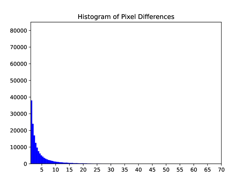
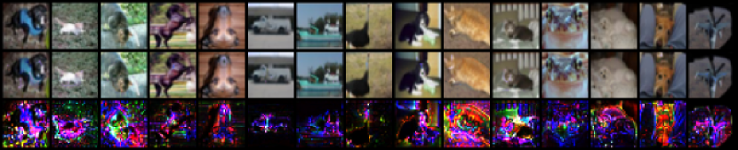
Figure 1: Adversarial images for pretrained TRADES on CIFAR10 training images. First row is the original image, second row is the adversarial image and last row is the normalized difference. Even though the model was trained to be robust to any perturbation in which all pixel values are less than $8/255$, it can be easily fooled by imperceptible perturbations in which almost all pixel values are less than $8/255$.

1 Introduction

Figure 1 illustrates the well-known phenomenon of adversarial examples[1]. The top row shows CIFAR10 images that are correctly classified by a convolutional neural network, and the middle row shows nearly identical images that are misclassified by the same network. The bottom row shows the difference between the original images and the adversarial images, where the difference has been rescaled. As can be seen in the histogram of the difference images, almost all pixels have been perturbed by a small amount (less than $\frac{8}{255}$). This intriguing property [1] of modern neural networks has attracted significant interest in fields such as computer vision [2], [3] [4], natural language processing [5], and cybersecurity [6].

Algorithms for adversarial training (e.g. [7, 8] ) try to address this lack of robustness of neural network classifiers by modifying the training procedure. At each iteration of training, the algorithms find adversarial examples of the current classifier, and minimize the loss with respect to these adversarial examples along with the loss on the original training examples. Algorithm 1 describes the powerful adversarial algorithm TRADES [7] which won the 1st place out of approximately 2,000 submissions in the NeurIPS 2018 Adversarial Vision Challenge. As we describe in the related work section, many state-of-the-art adversarial training methods are based on TRADES.

How well does adversarial training work? A commonly used metric is adversarial accuracy in which a classifier is said to correctly classify an image if it gives the correct output for all images in an $\epsilon$ ball around the image. Neural networks trained with standard training are highly vulnerable to small perturbations of their input so their adversarial accuracy is close to zero. For CIFAR10, adversarial training can increase the adversarial accuracy to above $60\%$ and with additional training data to above $70\%$ (e.g. [9], [10], [11]).

Despite the impressive progress in adversarial accuracy when using adversarial training, there are also several shortcomings. First, training using adversarial training is significantly more expensive, since an adversarial example needs to be found at each iteration of training. Second, the methods require several hyperparameters (e.g. the relative weights given to original examples vs. adversarial examples) and performance varies greatly with different choices. A third shortcoming is that adversarial training seems to mostly increase robustness to the specific types of perturbations that were used during training.

Figure 1 illustrates this last shortcoming. The adversarial examples that are shown are for a pretrained classifier that was trained with TRADES (downloaded from [12]). During training, the algorithm was shown adversarial training examples in which the perturbations have an $\ell_{\infty}$ norm of at most $8/255$, i.e. each pixel is perturbed by at most $8/255$ as is commonly used in the literature and indeed this pretrained classifier achieves an adversarial accuracy of over $54\%$ with these perturbations. However, when we slightly change the definition of allowed perturbations and allow perturbations whose $\ell_{2}$ norm is less than the $\ell_{2}$ norm of an image where all pixels have been perturbed by at most $8/255$ (i.e. $\ell_{2}$ less than $1.74$ in the case of CIFAR10 images) then the adversarial accuracy is less than $5\%$. In other words for more than $95\%$ of the images, the classifier that was trained with adversarial training can be fooled with an imperceptible change of the input image. This illustrates the fact that "most adversarial training methods can only defend against a specific attack that they are trained with. "[13].

In this paper we compare adversarial training to the simple 1 Nearest Neighbor (1NN) classifier. As motivation, consider the synthetic 2D classification problem shown in figure 2. When we train a neural network with standard training, it correctly classifies all the training examples but there are still several points that would not be robustly classified: the decision boundary passes through the $\ell_{\infty}$ ball around the training example. When we use TRADES, the result depends on the hyperparameters: in some settings all points are classified correctly but the decision boundary is similar to that obtained with normal training and in other settings (figure 2a) the robust accuracy is higher but still the decision boundary may pass through the $\ell_{\infty}$ ball around the training example. In contrast, the simple 1NN classifier (shown on the right) correctly classifies all training examples and any small perturbation of these examples.

The organization of this paper is as follows. We first theoretically analyze the 1NN classifier and show that under reasonable assumptions, the 1NN classifier will be robust to any small image perturbation of the training images and will give high adversarial accuracy on test images as the number of training examples goes to infinity. We then perform experiments with 45 different binary image classification problems taken from CIFAR10. We find that 1NN outperform TRADES in terms of average adversarial accuracy. In additional experiments with 69 pretrained robust models for CIFAR10, we find that 1NN outperforms almost all of them in terms of robustness to perturbations that are only slightly different from those seen during training. Taken together, our results suggest that modern adversarial training methods still fall short of the robustness of the simple 1NN classifier.

Algorithm 1 Adversarial training by TRADES

0:  Step sizes $\eta_{1}$ and $\eta_{2}$, batch size $m$, number of iterations $K$ in inner optimization, network architecture parametrized by $\theta$

0:  Robust network $f_{\theta}$

1:  Randomly initialize network $f_{\theta}$, or initialize network with pre-trained configuration

2:  repeat

3:     Read mini-batch $B=\{x_{1},\ldots,x_{m}\}$ from the training set

4:     for $i=1$ to $m$ (in parallel) do

5:        $x^{\prime}_{i}\leftarrow x_{i}+0.001\cdot\mathcal{N}(0,I)$, where $\mathcal{N}(0,I)$ is the Gaussian distribution with zero mean and identity variance

6:        for $k=1$ to $K$ do

7:           $x^{\prime}_{i}\leftarrow\Pi_{B_{(x_{i},\varepsilon)}}\left(\eta_{1}\cdot{\text{sign}}(\nabla_{x^{\prime}_{i}}L(f_{\theta}(x_{i}),f_{\theta}(x^{\prime}_{i})))+x^{\prime}_{i}\right)$ , where $\Pi$ is the projection operator

8:        end for

9:     end for

10:     $\theta\leftarrow\theta-\eta_{2}\sum_{i=1}^{m}\nabla_{\theta}\left[L(f_{\theta}(x_{i}),y_{i})+{L(f_{\theta}(x_{i}),f_{\theta}(x^{\prime}_{i}))}/{\lambda}\right]/m$

11:  until training converged

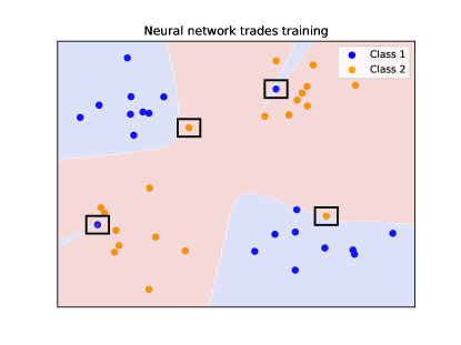
(a) TRADES

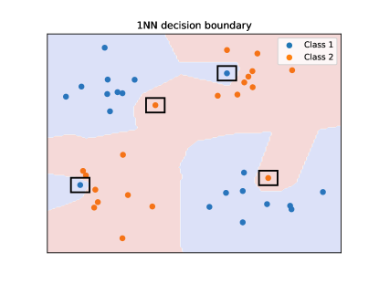
(b) 1NN

Figure 2: The decision boundary of TRADES (left) and 1NN on a simple 2D classification problem. The black square denotes the $\epsilon$ ball that defines adversarial accuracy (for which TRADES was trained). TRADES succeeds in making the decision boundary constant within the $\epsilon$ ball for some examples but not all. In contrast, the 1NN classifier achieves high robustness to any small perturbation of the training examples.

2 The Robust Accuracy of 1NN

3 The Robust Accuracy of 1NN

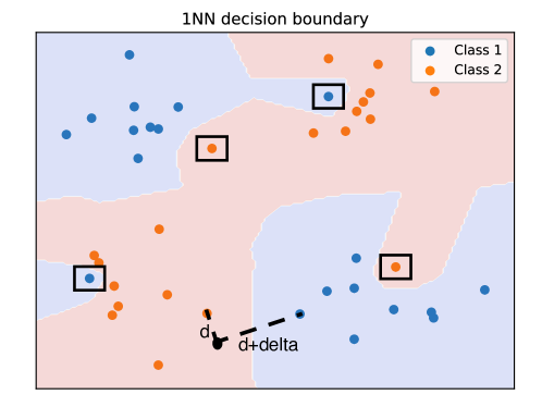
Figure 3: Illustration of the proof of theorem 1. If the distance to the closest point in the correct class is $d$ and the closest point in the incorrect class is $d+\delta$ then the 1NN classifier will be robust to any perturbation smaller than $\delta/2$.

The 1NN classifier has been extensively studied in machine learning (e.g. [14]) and is known to achieve a generalization error that is at most twice that of the Bayes optimal classifier as the number of examples goes to infinity. In the context of adversarial examples, the 1NN classifier has an additional advantage that it allows exact computation of the adversarial accuracy. Recall that in adversarial accuracy, a classifier is said to correctly classify an example if it outputs the correct label for all inputs in an $\epsilon$ ball around the example. For a neural network classifier, there is no way for us to determine if a given example will be robustly classified. Rather, we can only employ a local search algorithm that searches for an adversarial example within the $\epsilon$ ball. In contrast, we now show how to determine the adversarial accuracy of the 1NN classifier exactly.

Definition 3.1.

The 1NN classifier is a function that returns for each $x$, the class of $x_{NN}$ where $x_{NN}=\arg\min_{j}d(x,x_{j})$ is the closest training example to $x$ in terms of $\ell_{2}$ norm.

Definition 3.2.

The $\epsilon$ adversarial accuracy of a classifier $f(x)$ on a set of examples $X=\{x_{i},y_{i}\}_{i=1}^{N}$ with an $\ell_{p}$ norm is:

$$RA(X,\delta,p;f)=\frac{1}{N}\sum_{i}\min_{v:\|v\|_{p}<\epsilon}[f(x_{i}+v)==y_{i}]$$ (1)

Given these definitions we now show that the 1NN classifier will be provably robust to any small perturbations for test examples for which it is "confident", i.e. the nearest neighbor from the true class is significantly closer than the nearest neighbor from another class.

Definition 3.3.

$\delta$ 1NN Confident test examples. A test example is $\delta$ confidently classified by the 1NN classifier if $d(x,x_{1})>d(x,x_{0})-\delta$ where $x_{0}$ is the closest example in the correct class and $x_{1}$ is the closest example in another class.

For points for which the 1NN classifier, it is easy to show that it will be robust to small perturbations. The following theorem formalizes this intuition.

Theorem 1.

Denote by $X_{c}$ a set of examples that are $\delta$ confidently classified by the 1NN classifier. The $\delta/2$ robust accuracy of the 1NN classifier on this set with $\ell_{2}$ norm is $100\%$:

$$RA(X_{c},\delta/2,2;1NN)=1$$

Proof.

The proof is based on the triangle inequality and is illustrated graphically in figure 3. A full proof is given in the appendix. ∎

We now turn to characterizing conditions under which certain points will be confidently characterized by the 1NN classifier. We use the notion of the distance between the two classes: the minimal distance between a point in one class and a point in the other class. The larger that this distance is, the more confident the 1NN classifier will be in its prediction. This leads to the following theorem.

Theorem 2.

for 1NN classifier if the distance between two classes is $d_{0}$ then $\frac{d_{0}}{2}$ adversarial accuracy with $\ell_{2}$ norm is $100\%$ over the training samples

This theorem follows directly from theorem 1. At first glance, guaranteeing robustness for training examples seems trivial, but note that for many modern classifiers, even the output on the training images can be changed with a tiny perturbation of the input. Specifically, all the examples in figure 1 are training images and yet a neural network that is trained using the state of the art adversarial training algorithm can be fooled with tiny perturbations. The following theorem shows that the same property holds for test examples, but only when the number of training examples goes to infinity,

Theorem 3.

for 1NN classifier if the distance between two classes is $d_{0}$ then $\frac{d_{0}}{2}$ adversarial accuracy with $\ell_{2}$ norm is $100\%$ over the test samples as the number of training examples goes to infinity,

This theorem follows from the fact that as the number of training examples goes to infinity, the distance of a test example to the nearest neighbor in the same class goes to zero. This is the same property that is used to analyze the asymptotic performance of the 1NN classifier [14].

The theory so far has focused on perturbations where the adversary is constrained to an $\epsilon$ ball in $\ell_{2}$. What happens with other $p$ norms? The easiest case is when $p\leq 2$.

Corollary 3.1.

for any $\text{p}\leq 2$, if the $\ell_{2}$ distance between the two classes is $d_{0}$ then $\frac{d_{0}}{2}$ adversarial accuracy with $\ell_{p}$ norm is $100\%$ on the training examples

Corollary 3.2.

for any $\text{p}\leq 2$ the $\frac{\delta}{2}$ adversarial accuracy of test examples that are classified $\delta$ confidently is $100\%$.

Both of these follow from the fact that the unit ball with $\ell_{p}$ norm is contained within the unit ball with $\ell_{2}$ norm for any $p\leq 2$

Finally, we can summarize all of our results for all $p$ norms in the following corollary:

Corollary 3.3.

Suppose that the $\ell_{2}$ distance between the two classes is $2\delta\sqrt{N}$ where N is the dimensionality. For any p the $\delta$ adversarial accuracy is $100\%$ on the training set and as the number of examples goes to infinity the $\delta$ adversarial accuracy on the test set will also be $100\%$

Proof.

This follows from the fact that for any p the $\ell_{p}$ unit ball is contained within the $\ell_{\infty}$ unit ball and the $\delta$ ball for $\ell_{\infty}$ is contained within the $\sqrt{N}\delta$ ball for $\ell_{2}$ ∎

How realistic are the assumptions of our theorems? As we mentioned in the introduction, it is common to assume that any two images in which the difference in each pixel is at most $\delta$ are perceptually indistinguishable. If we also assume rotation invariance, this implies that any two images separated by a vector whose $\ell_{2}$ norm is less than $\delta\sqrt{N}$ are perceptually indistinguishable. Thus if there exists two examples of different classes that are separated by only $2\delta\sqrt{N}$, this would mean that the image halfway between the two examples is perceptually indistinguishable from both images, even though they are images of different objects. In other words, we expect the assumption that the training examples in the two classes are separated by at least $2\delta\sqrt{N}$ to hold in realistic datasets. The second assumption in theorem 2, however, is that the number of training examples goes to infinity, and this is problematic. In the next section, we evaluate how well 1NN performs on real datasets with finite number of examples.

4 Experiments

To evaluate the performance of 1NN and adversarial training on real datasets, we carried out an extensive series of experiments. In our first experiments we divided the CIFAR-10 dataset into 45 subsets, representing all possible pairs. For each subset, we compared the robust accuracy of the following algorithms:

1. The 1NN classifier

2. TRADES with recommended hyperparameters based on a ResNet18 architecture (as in [15]). We refer to this algorithm as T_R in the figures.

3. TRADES with the best hyperparameters. For each of the 45 problems, We tried 600 possible combinations of the hyperparameters and chose the one that gave highest adversarial accuracy. We refer to this algorithm as T_B.

4. Standard training of the same ResNet18 architecture. We refer to this algorithm as S.

5. Standard training with early stopping (20 epochs). we refer to this algorithm as E_S.

6. A version of TRADES which attempts to be robust to both $\ell_{\infty}$ and $\ell_{2}$ attacks. In this version, at each iteration we inject two adversarial examples into the training set: one is constrained to be within the $\ell_{2}$ ball around the original example and the second is constrained to be within the $\ell_{\infty}$ ball. We refer to this algorithm as T_B_A.

As mentioned above, for the 1NN classifier we can calculate the robust accuracy exactly but to evaluate the CNN’s robust accuracy we need to perform optimization. We primarily used the RobustBench standard APGD-CE[16] attack. In some instances, we also tested with tools like CleverHans[17] and Foolbox[18]. However, our assessments indicated that RobustBench was either equally effective or superior in compromising the same or a higher number of samples compared to the other tools, and the evaluation was faster.

Table 1 shows the training and inference times for each relevant method. For the 1NN we used the FAISS package [19] which builds an index over the training example in order to facilitate fast nearest neighbor search and we use that as the equivalent of "training time". Clearly 1NN is orders of magnitude faster.

Table 1: Running Times for Training and Inference, on GeForce RTX 2080 Ti, with ResNet18 over binary cifar10 problem

Algorithm	Training Time (seconds)	Inference Time (seconds)
TRADES	$7467.693$	$0.000\,09$
early stop	$99.842\,68$	$0.000\,09$
1NN faiss	$0.340\,34$	$0.000\,01$

On all 45 problems we evaluated the algorithms using the following criteria. First we evaluated all algorithms using clean accuracy (Figure LABEL:sub@subfig:fig1_rob). As expected the 1NN classifier is quite poor using this measure and is much worse than the CNN. We then asked about the adversarial accuracy when we either constrain the attacker to the $\ell_{\infty}$ ball with the standard $\delta=\frac{8}{255}$ or we constrain the attacker to the $\ell_{2}$ ball with $\delta=\frac{8}{255}\sqrt{3072}$. We measured the adversarial accuracy separately on the training set and the test set.

As predicted by our theorems, the 1NN achieves 100% robust accuracy on the training set while none of the other algorithms are above 40% $\ell_{2}$ robust accuracy or $80\%$ $\ell_{\infty}$ robust accuracy on the train. Thus robust training fails to even learn how to robustly classify the training examples.

When comparing robust accuracy on the test set the results depend on the norm. When we use $\ell_{2}$ robust accuracy the simple 1NN is better than all versions of TRADES and when we use $\ell_{\infty}$ it is comparable to the best version of TRADES. As a consequence when we use both measures together the simple 1NN is the best algorithm in terms of robust accuracy on the test set. Figure 6 shows that the simple 1NN indeed outperforms the best version of TRADES in the majority of 45 experiments (36), not just in the average over all 45 experiments.

In addition to the 45 experiments described above we also compared the performance of 69 state-of-the-art pretrained models (all of the available CIFAR10, $\ell^{\infty}$ models at [12]) to that of the simple 1NN classifier. These pretrained models include a range of architectures and algorithms that are built on the basis of adversarial training but also include methods that take advantage of additional training data (e.g. one of the current leaders uses 50 Million images generated by a diffusion model in addition to the CIFAR10 images [20]).

As seen in figure 2 the behaviour is similar to what we saw in the binary experiments: the simple 1NN is better than almost all the pretrained models in terms of $\ell_{2}$ robust accuracy and in terms of $\ell_{\infty}$ accuracy on the training set. Thus even when the models are trained with millions of additional images and adversarially generated examples, they still fail to be robust for small perturbations that are only slightly different from those seen during training. In contrast, the 1NN classifier is robust to any small perturbation as predicted by our theory.

Figure 7 shows the adversarial examples needed to fool the 1NN classifier for the same training examples of the pretrained TRADES model. It can be seen that the changes required to fool the model are much larger and almost all pixels should be changed by over $\frac{8}{255}$.

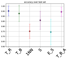
(a) Clean Accuracy

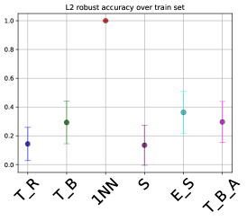
(b) $\ell_{2}$ robust accuracy train

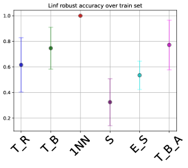
(c) $\ell_{\infty}$ robust accuracy train

Figure 4: Comparison of different algorithms on 45 CIFAR10 subproblems using clean accuracy and robust accuracy on the training set. The simple 1NN algorithm is the only one that achieves 100% robust accuracy on the training set even though it is worst in terms of clean accuracy.

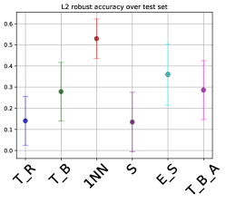
(a) $\ell_{2}$ Robust Accuracy Test

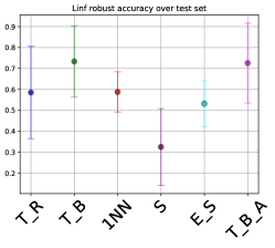
(b) $\ell_{\infty}$ Robust Accuracy Test

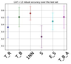
(c) $\ell_{\infty}+\ell_{2}$ Robust Accuracy Test

Figure 5: Comparison of different algorithms on 45 CIFAR10 subproblems using robust accuracy on the test set. The simple 1NN algorithm is better than all versions of TRADES when both $\ell_{2}$ and $\ell_{\infty}$ robustness are considered.

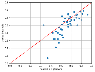
Figure 6: Summary of the results of all 45 experiments. Each dot represents an experiment and the two coordinates are the $\ell_{\infty}+\ell_{2}$ Robust Accuracy. In 36 out of the 45 problems, the 1NN is better or comparable to the best values of TRADES.

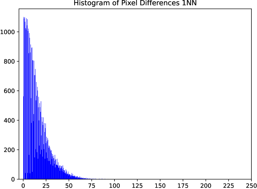
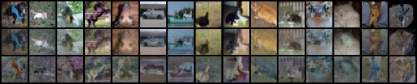
Figure 7: Adversarial images for 1NN for the same CIFAR10 training images shown in 1. First row is the original image, second row is the adversary image and last line is the normalized difference. As can be seen in the histogram of pixel differences on top, to fool the 1NN nearest neighbor classifier, almost all pixels should be changed by over $8/255$.

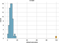
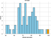
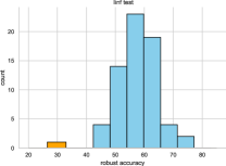
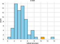
$\ell_{2}$ RA train $\ell_{\infty}$ RA train $\ell_{\infty}$ RA test $\ell_{2}$ RA test

Figure 8: Comparison of 1NN (yellow) and 69 pretrained models for CIFAR10 downloaded from the current $\ell_{\infty}$ robustness leaderboard (blue). All models are trained using adversarial training using $\ell_{\infty}$ attacks and indeed they increase the adversarial accuracy using this measure significantly. However, when these models are evaluated using $\ell_{2}$ attacks, they are inferior to the 1NN classifier.

5 Related Work

In our work we mostly focused on TRADES as an example of adversarial training. Many recent papers are based on variations of TRADES. For example [21] add momentum and weights vector to the TRADES loss, FAT [22] seems to get best results when incorporated with TRADES or with MART([23]), [24] uses teacher model to guide the robust model, [25] adds hypersphere embedding mechanism. MART uses BCE instead of CE and weights the logits logsumexp probabilities as a new weight vector, [26] improved the KL-divergance term. [27] uses another network to choose the attack strategy. [28] uses teacher model instead of natural labels, [29] uses TRADES+AWP as their base algorithm and additionally minimize the Jenson-Shannon (JS) divergence between the softmax outputs of different augmentations. [30] adds weights to the loss according to the geometry value of data, which is the least number of iterations that PGD needs to find its misclassified adversarial variant. AWP [31] perturb the model weights, along the direction in which which the adversarial loss increases dramatically as part of the training scheme and is added as an extra step in several works. [32] change the optimizer scheduler [33] mostly asks about the perturbation stability of the networks as a factor of the width, and offer Width Adjusted Regularization algorithm that takes into account the ratio between the stable samples and all of the training set. [34] explored the architectural ingredients of adversarially robust DNNs. [35] adds helper samples and new loss the TRADES optimization process. [36] uses TRADES embeddings. [9] focus on analyzing the role of architectural elements on adversarial robustness when using adversarial training. [37] add weight averaging, enlarge the model, changes the activation’s and changes the scheduler, but uses TRADES as their framework. and [38] showed that combining heuristics-based data augmentations with model weight averaging can significantly improve robustness when trained with TRADES framework.

6 Discussion

Despite the large amount of attention that the research community has invested in adversarial examples, the problem is still unsolved and even state of the art methods based on adversarial training can be easily fooled with tiny perturbations of the input. In this paper we have compared adversarial training to the simple 1NN classifier. We have analyzed the 1NN classifier and shown proven that under reasonable assumptions, the 1NN will have 100% adversarial accuracy on the training set and as the number of training examples goes to infinity, it will also attain 100% adversarial accuracy on the test set for any $p$ norm. In extensive experiments on 45 different image classification problems, the simple 1NN classifier outperforms adversarial training in terms of robust accuracy when both $\ell_{2}$ and $\ell_{\infty}$ norms are used.

We see the simple 1NN classifier as an example of a simple algorithm that provides robustness to any small perturbation and therefore serves as an alternative to adversarial training. We do not, however, advocate using the 1NN classifier in pixel space for image classification since obviously the performance for finite training data is far from state-of-the-art. We believe that there are more powerful algorithms that are based on 1NN in other feature spaces that can improve accuracy and still guarantee robustness and this is a promising direction for future research.

Appendix

Detailed of proof of theorem 1.

Denote by $d(x+v,A)$ the distance to the correct class and $d(x+v,B)$ the distance to the other class. We want to show that $d(x+v,A)<d(x+v,B)$ for any $v$ such that $\|v\|<\delta/2$. Since $d(x,A)=d(x,x_{0})$ we have that:

$$d(x+v,A) = \min_{i\in A}d(x+v,x_{i})$$ (2)

$$\leq \min_{i\in A}d(x,x_{i})+\frac{\delta}{2}$$ (3)

$$= d(x,x_{0})+\frac{\delta}{2}$$ (4)

and similarly:

$$d(x+v,B) = \min_{i\in B}d(x+v,x_{i})$$ (5)

$$\geq \min_{i\in B}d(x,x_{i})-\frac{\delta}{2}$$ (6)

$$= d(x,x_{1})-\frac{\delta}{2}$$ (7)

and since the example is $\delta$ confident $d(x,x_{1})>d(x,x_{0})-\delta$ so that $d(x+v,A)<d(x+v,B)$.

References

- [1] Christian Szegedy, Wojciech Zaremba, Ilya Sutskever, Joan Bruna, Dumitru Erhan, Ian Goodfellow, and Rob Fergus. Intriguing properties of neural networks. arXiv preprint arXiv:1312.6199, 2013.
- [2] Ian J Goodfellow, Jonathon Shlens, and Christian Szegedy. Explaining and harnessing adversarial examples. arXiv preprint arXiv:1412.6572, 2014.
- [3] Nicolas Papernot, Patrick McDaniel, and Ian Goodfellow. Transferability in machine learning: from phenomena to black-box attacks using adversarial samples. arXiv preprint arXiv:1605.07277, 2016.
- [4] Nicholas Carlini and David Wagner. Towards evaluating the robustness of neural networks. In 2017 ieee symposium on security and privacy (sp), pages 39–57. Ieee, 2017.
- [5] Andy Zou, Zifan Wang, J Zico Kolter, and Matt Fredrikson. Universal and transferable adversarial attacks on aligned language models. arXiv preprint arXiv:2307.15043, 2023.
- [6] Naghmeh Moradpoor, Leandros Maglaras, Ezra Abah, and Andres Robles-Durazno. The threat of adversarial attacks against machine learning-based anomaly detection approach in a clean water treatment system. In 2023 19th International Conference on Distributed Computing in Smart Systems and the Internet of Things (DCOSS-IoT), pages 453–460. IEEE, 2023.
- [7] Hongyang Zhang, Yaodong Yu, Jiantao Jiao, Eric Xing, Laurent El Ghaoui, and Michael Jordan. Theoretically principled trade-off between robustness and accuracy. In International conference on machine learning, pages 7472–7482. PMLR, 2019.
- [8] Aleksander Madry, Aleksandar Makelov, Ludwig Schmidt, Dimitris Tsipras, and Adrian Vladu. Towards deep learning models resistant to adversarial attacks. arXiv preprint arXiv:1706.06083, 2017.
- [9] Shihua Huang, Zhichao Lu, Kalyanmoy Deb, and Vishnu Naresh Boddeti. Revisiting residual networks for adversarial robustness: An architectural perspective. arXiv preprint arXiv:2212.11005, 2022.
- [10] Zekai Wang, Tianyu Pang, Chao Du, Min Lin, Weiwei Liu, and Shuicheng Yan. Better diffusion models further improve adversarial training. In International Conference on Machine Learning, pages 36246–36263. PMLR, 2023.
- [11] ShengYun Peng, Weilin Xu, Cory Cornelius, Matthew Hull, Kevin Li, Rahul Duggal, Mansi Phute, Jason Martin, and Duen Horng Chau. Robust principles: Architectural design principles for adversarially robust cnns. arXiv preprint arXiv:2308.16258, 2023.
- [12] Francesco Croce, Maksym Andriushchenko, Vikash Sehwag, Edoardo Debenedetti, Nicolas Flammarion, Mung Chiang, Prateek Mittal, and Matthias Hein. RobustBench: a standardized adversarial robustness benchmark. In Thirty-fifth Conference on Neural Information Processing Systems Datasets and Benchmarks Track, 2021.
- [13] Weili Nie, Brandon Guo, Yujia Huang, Chaowei Xiao, Arash Vahdat, and Anima Anandkumar. Diffusion models for adversarial purification. arXiv preprint arXiv:2205.07460, 2022.
- [14] Richard O Duda, Peter E Hart, et al. Pattern classification. John Wiley & Sons, 2006.
- [15] Tianyu Pang, Xiao Yang, Yinpeng Dong, Hang Su, and Jun Zhu. Bag of tricks for adversarial training. arXiv preprint arXiv:2010.00467, 2020.
- [16] Francesco Croce and Matthias Hein. Reliable evaluation of adversarial robustness with an ensemble of diverse parameter-free attacks. In International conference on machine learning, pages 2206–2216. PMLR, 2020.
- [17] Nicolas Papernot, Fartash Faghri, Nicholas Carlini, Ian Goodfellow, Reuben Feinman, Alexey Kurakin, Cihang Xie, Yash Sharma, Tom Brown, Aurko Roy, Alexander Matyasko, Vahid Behzadan, Karen Hambardzumyan, Zhishuai Zhang, Yi-Lin Juang, Zhi Li, Ryan Sheatsley, Abhibhav Garg, Jonathan Uesato, Willi Gierke, Yinpeng Dong, David Berthelot, Paul Hendricks, Jonas Rauber, and Rujun Long. Technical report on the cleverhans v2.1.0 adversarial examples library. arXiv preprint arXiv:1610.00768, 2018.
- [18] Jonas Rauber, Roland Zimmermann, Matthias Bethge, and Wieland Brendel. Foolbox native: Fast adversarial attacks to benchmark the robustness of machine learning models in pytorch, tensorflow, and jax. Journal of Open Source Software, 5(53):2607, 2020.
- [19] Jeff Johnson, Matthijs Douze, and Hervé Jégou. Billion-scale similarity search with GPUs. IEEE Transactions on Big Data, 7(3):535–547, 2019.
- [20] Zekai Wang, Tianyu Pang, Chao Du, Min Lin, Weiwei Liu, and Shuicheng Yan. Better diffusion models further improve adversarial training. In Andreas Krause, Emma Brunskill, Kyunghyun Cho, Barbara Engelhardt, Sivan Sabato, and Jonathan Scarlett, editors, Proceedings of the 40th International Conference on Machine Learning, volume 202 of Proceedings of Machine Learning Research, pages 36246–36263. PMLR, 23–29 Jul 2023.
- [21] Lang Huang, Chao Zhang, and Hongyang Zhang. Self-adaptive training: beyond empirical risk minimization. Advances in neural information processing systems, 33:19365–19376, 2020.
- [22] Jingfeng Zhang, Xilie Xu, Bo Han, Gang Niu, Lizhen Cui, Masashi Sugiyama, and Mohan Kankanhalli. Attacks which do not kill training make adversarial learning stronger. In International conference on machine learning, pages 11278–11287. PMLR, 2020.
- [23] Yisen Wang, Difan Zou, Jinfeng Yi, James Bailey, Xingjun Ma, and Quanquan Gu. Improving adversarial robustness requires revisiting misclassified examples. In International conference on learning representations, 2019.
- [24] Jiequan Cui, Shu Liu, Liwei Wang, and Jiaya Jia. Learnable boundary guided adversarial training. In Proceedings of the IEEE/CVF international conference on computer vision, pages 15721–15730, 2021.
- [25] Tianyu Pang, Xiao Yang, Yinpeng Dong, Kun Xu, Jun Zhu, and Hang Su. Boosting adversarial training with hypersphere embedding. Advances in Neural Information Processing Systems, 33:7779–7792, 2020.
- [26] Jiequan Cui, Zhuotao Tian, Zhisheng Zhong, Xiaojuan Qi, Bei Yu, and Hanwang Zhang. Decoupled kullback-leibler divergence loss. arXiv preprint arXiv:2305.13948, 2023.
- [27] Xiaojun Jia, Yong Zhang, Baoyuan Wu, Ke Ma, Jue Wang, and Xiaochun Cao. Las-at: adversarial training with learnable attack strategy. In Proceedings of the IEEE/CVF Conference on Computer Vision and Pattern Recognition, pages 13398–13408, 2022.
- [28] Erh-Chung Chen and Che-Rung Lee. Ltd: Low temperature distillation for robust adversarial training. arXiv preprint arXiv:2111.02331, 2021.
- [29] Sravanti Addepalli, Samyak Jain, et al. Efficient and effective augmentation strategy for adversarial training. Advances in Neural Information Processing Systems, 35:1488–1501, 2022.
- [30] Jingfeng Zhang, Jianing Zhu, Gang Niu, Bo Han, Masashi Sugiyama, and Mohan Kankanhalli. Geometry-aware instance-reweighted adversarial training. arXiv preprint arXiv:2010.01736, 2020.
- [31] Dongxian Wu, Shu-Tao Xia, and Yisen Wang. Adversarial weight perturbation helps robust generalization. Advances in Neural Information Processing Systems, 33:2958–2969, 2020.
- [32] Kaustubh Sridhar, Oleg Sokolsky, Insup Lee, and James Weimer. Improving neural network robustness via persistency of excitation. In 2022 American Control Conference (ACC), pages 1521–1526. IEEE, 2022.
- [33] Boxi Wu, Jinghui Chen, Deng Cai, Xiaofei He, and Quanquan Gu. Do wider neural networks really help adversarial robustness? Advances in Neural Information Processing Systems, 34:7054–7067, 2021.
- [34] Hanxun Huang, Yisen Wang, Sarah Erfani, Quanquan Gu, James Bailey, and Xingjun Ma. Exploring architectural ingredients of adversarially robust deep neural networks. Advances in Neural Information Processing Systems, 34:5545–5559, 2021.
- [35] Rahul Rade and Seyed-Mohsen Moosavi-Dezfooli. Helper-based adversarial training: Reducing excessive margin to achieve a better accuracy vs. robustness trade-off. In ICML 2021 Workshop on Adversarial Machine Learning, 2021.
- [36] Qiyu Kang, Yang Song, Qinxu Ding, and Wee Peng Tay. Stable neural ode with lyapunov-stable equilibrium points for defending against adversarial attacks. Advances in Neural Information Processing Systems, 34:14925–14937, 2021.
- [37] Sven Gowal, Chongli Qin, Jonathan Uesato, Timothy Mann, and Pushmeet Kohli. Uncovering the limits of adversarial training against norm-bounded adversarial examples. arXiv preprint arXiv:2010.03593, 2020.
- [38] Sylvestre-Alvise Rebuffi, Sven Gowal, Dan A Calian, Florian Stimberg, Olivia Wiles, and Timothy Mann. Fixing data augmentation to improve adversarial robustness. arXiv preprint arXiv:2103.01946, 2021.