20XX Vol. X No. XX, 000–000
22institutetext: University of Chinese Academy of Sciences, Beijing, 100049, P.R.China
33institutetext: Institute for Frontiers in Astronomy and Astrophysics, Beijing Normal University, Beijing, 102206, P.R.China
\vs\noReceived 2024 Month Day; accepted 2024 Month Day
Dynamical dark energy in light of cosmic distance measurements II: a study using current observations
Abstract
We extract key information of dark energy from current observations of BAO, OHD and , and find hints of dynamical behaviour of dark energy. In particular, a dynamical dark energy model whose equation of state crosses is favoured by observations. We also find that the Universe has started accelerating at a lower redshift than expected.
keywords:
Cosmic Expansion History — Large-scale-structure — Baryon Acoustic Oscillations; Type Ia supernova1 INTRODUCTION
The physical origin of the cosmic acceleration remains unveiled since its discovery in from observations of supernovae Type Ia (SNe Ia) (Riess et al. 1998; Perlmutter et al. 1999). Among all possible mechanisms, dark energy (DE) (Copeland et al. 2006) and modified gravity (MG) (Clifton et al. 2012) are two primary scenarios that have been extensively studied. Both DE and MG models can yield the same accelerating expansion of the Universe after the required tuning, and the expansion rate of the Universe is determined by the equation of state (EoS) of an effective dark fluid.
The EoS is generally a function of time, expressed by the scale factor or redshift , and it is a ratio between the pressure and of the effective dark fluid. It is important to extract information of from observations, because different DE or MG theory models can in principle be differentiated using the behaviour of . The CDM model, in which dark energy is the vacuum energy, predicts . Although still allowed by observations, this model suffers from serious theory problems (Weinberg 1989), and has been challenged by the ‘Hubble tension’ (Di Valentino et al. 2021). In alternative models, generally evolves with time. For example, the single-scalar-field models of quintessence (Ratra & Peebles 1988) and phantom (Caldwell 2002) predict and during the evolution, respectively, and in models with intrinsic degrees of freedom such as quintom (Feng et al. 2005), can cross the boundary.
Observations of the cosmic distances, such as the baryonic acoustic oscillations (BAO) (Eisenstein & Hu 1998; Eisenstein et al. 2005; Cole et al. 2005), are less subject to systematics compared to probes of the cosmic structure formation, and the behaviour of directly affects the cosmic distances, therefore the distance measurements are ideal observables for dark energy studies.
In this work, we learn the behaviour of from current measurements of the cosmic distances based on the method developed in a companion paper (Gu et al. 2024), and find hints of interesting features of . We present the method and data used in this analysis in Sec. 2, show the result in Sec. 3 and conclude in Sec. 4.
2 Method and Data
In this section, we briefly describe the method used for this work, as developed in a companion paper (Gu et al. 2024), and the datasets used for the analysis.
We start from parametrising the angular diameter distances111For current data, we find that keeping the expansion up to the term is a reasonable choice to balance between the bias and uncertainty of the reconstruction. following Zhu et al. (2015),
| (1) |
where , and subscript ‘fid’ denotes the fiducial model, which is chosen to be a flat CDM model with as favoured by the Planck observations (Aghanim et al. 2020). The quantity is the pivot redshift set to in this work222The choice of can be arbitrary in principle, and it has almost no impact on the final reconstruction result, as demonstrated in Gu et al. (2024).. The Hubble expansion rate can be obtained using the relation between and , namely,
| (2) |
The free parameters can be determined by fitting Eqs. (1) and (2) to distance measurements, generally including BAO and supernovae distances, the observational Hubble data (OHD) (Stern et al. 2010) and so forth. Ultimately we can obtain a dark energy shape function defined as,
| (3) |
Throughout the paper, the prime denotes a derivative with respect to the scale factor , and is the dark energy density normalised to unity today333Note that when fitting the ’s in Eqs. (1) and (2) to distance measurements, the derived may not be positive-definite. Therefore when deriving quantities related to including the pressure function and the function, we apply a prior of . We check the posteriors and find that this has a marginal effect on the final result.. By design, extracts the shape of from data, thus constants are irrelevant444For BAO measurements, where is the sound horizon at decoupling. But these constants have no impact on and by design.. A few important functions that are directly related to dark energy can be derived from , including the normalised dark energy pressure function,
| (4) |
and the dark energy characterisation function,
| (5) |
Given , a general solution to the differential equation (5) is,
| (6) |
with
| (7) |
and is the boundary condition at .
In addition, the deceleration function of the Universe can also be derived from , namely,
| (8) |
The datasets used in this work include the isotropic and anisotropic BAO measurements listed in Table 1555Note that the BOSS and WiggleZ surveys have a small overlapping region in footprint thus the BAO measurements from these two surveys are not strictly independent. But given the small overlapping area compared to the full footprint of BOSS, we assume that the cross-covariance in the measurements is negligible., the observational data (OHD) measured using the ages of galaxies (Stern et al. 2010), compiled in Yu et al. (2018), and a local measurement of (Riess et al. 2022).
| Survey | Reference | ||||
|---|---|---|---|---|---|
| SDSS MGS | Ross et al. (2015) | ||||
| BOSS | Alam et al. (2017) | ||||
| BOSS | Alam et al. (2017) | ||||
| eBOSS LRG | Bautista et al. (2020) | ||||
| eBOSS ELG | de Mattia et al. (2021) | ||||
| eBOSS Quasar | Neveux et al. (2020) | ||||
| eBOSS Ly | du Mas des Bourboux et al. (2020) | ||||
| 6dFGS | Beutler et al. (2011) | ||||
| WiggleZ | Kazin et al. (2014) | ||||
| WiggleZ | Kazin et al. (2014) | ||||
| WiggleZ | Kazin et al. (2014) | ||||
| DES Y3 | Abbott et al. (2022) |
3 RESULTS
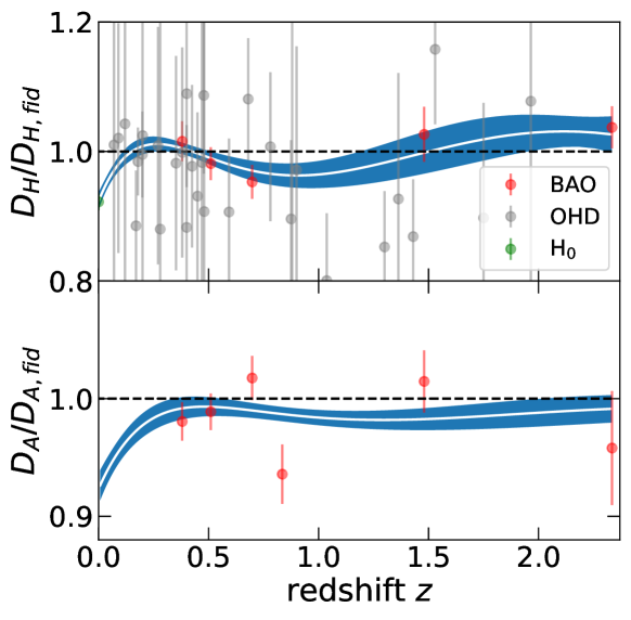
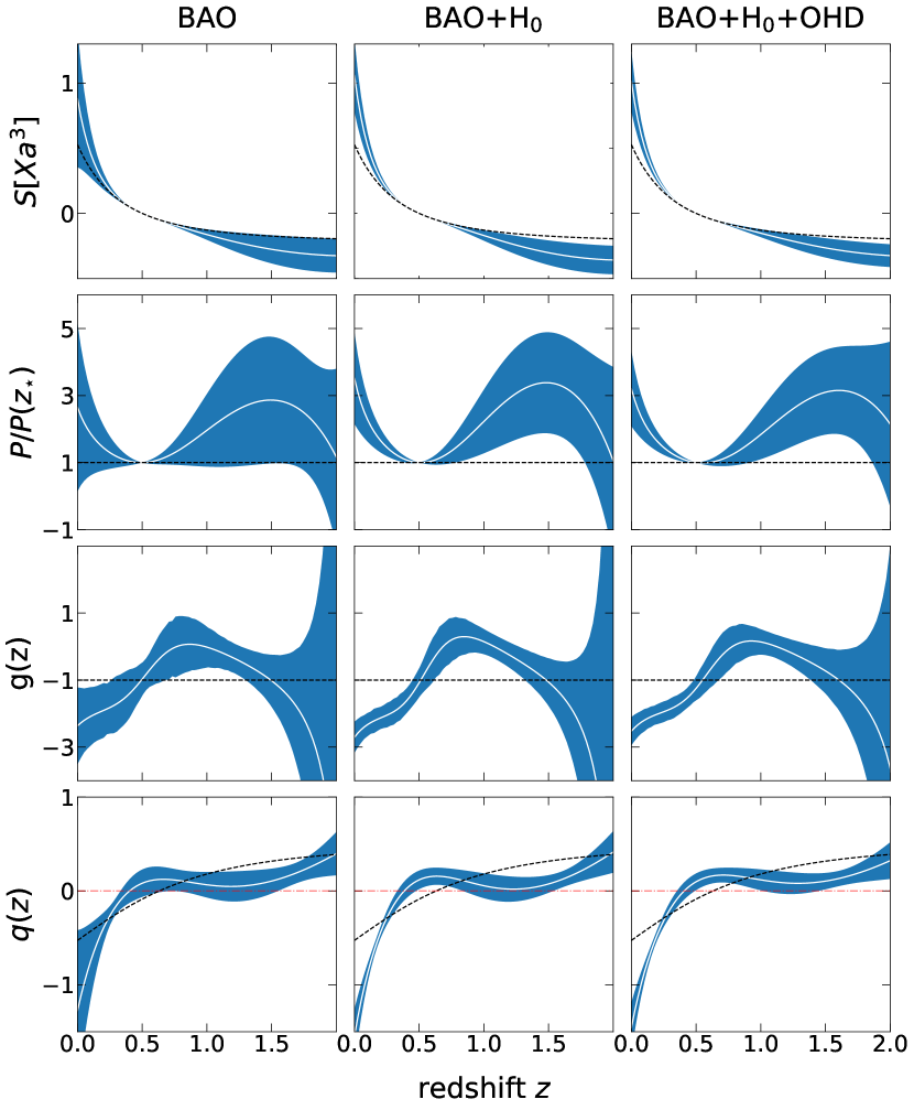
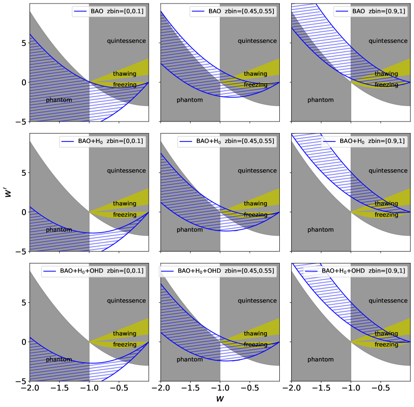
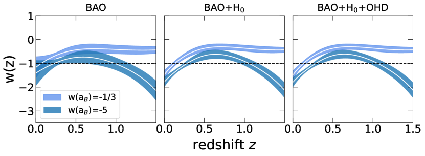
Fig. 1 shows the mean and 68% confidence level (CL) reconstructed ( is the speed of light) and from the combined dataset of BAO, OHD and measurements, rescaled by the prediction of the fiducial model. As shown, the reconstructed functions significantly deviate from the fiducial CDM model, and appear wiggly, which is primarily driven by both the and BAO measurements at low and intermediate redshifts, respectively.
Fig. 2 turns the distance measurements into important functions that are directly related to physical features of dark energy. Panels in the top row show the reconstructed dark energy shape function, visualising the time evolution of . Comparing to the CDM prediction shown in the black dashed lines, we see that the BAO data tilt around the pivot point of , namely, the BAO data tend to lift up at and push downwards at . Interestingly, this feature is supported by both the and OHD measurements, namely, when and OHD are added to the analysis, the feature becomes more pronounced with much smaller uncertainties, which disfavours the CDM model.
The panels provide more information of dark energy. Specifically, we see that has an apparent local minimum at around when the and OHD measurements are combined with the BAO data. This actually disfavours the CDM model, in which is a power-law function of .
Further information of can be learned from the reconstructed function shown in panels in the third row of Fig. 2. This function shows a strong dynamical behaviour in all cases, indicating an evolving . It is true that solving for from requires a boundary condition which is unknown, but we can still use the reconstructed to identify the allowed region in the phase space, which can in principle be used to differentiate dark energy models. The shaded area in Fig. 3 illustrate the allowed parameter space by single scalar field models. Specifically, the quintessence (Ratra & Peebles 1988) and phantom (Caldwell 2002) models sit in regions of and , respectively (Chiba 2006). The behaviour of the quintessence model may be classified into two scenarios, namely, the thawing ( at high redshifts and grows later on) and freezing ( at high redshifts and decreases with time) cases, occupying the regions of and , respectively (Caldwell & Linder 2005). On the other hand, the reconstructed function constrains the relation between and in a given redshift range, thus we can use to target the region in the phase space favoured by observations. In Fig. 2, the hatched regions are favoured by observations (at 68% CL) derived from different data combinations in three redshift intervals, namely, and . For all data combinations, we see a similar trend, namely, data favour the phantom model at , while at , most of the data-favoured region overlaps with the quintessence regime. This indicates an evolving that crosses the boundary during evolution, which is consistent with the prediction of the quintom model (Feng et al. 2005). We check this conclusion by directly solving the differential equation with two choices of boundary conditions, namely, and with , which are sufficiently extreme. The two solutions are shown in Fig. 4. In all cases, tends to cross during evolution, and the trend becomes significant when and OHD datasets are combined with the BAO data in the analysis.
Panels in the bottom row of Fig. 2 show the reconstructed deceleration function . Comparing to the CDM prediction with , we see that data favour a smaller , which is the redshift for the acceleration-deceleration transition, namely, while . This means that the Universe starts accelerating much later than expected in the CDM model.
4 CONCLUSION
Revealing the nature of dark energy is one of the most challenging tasks in modern physics. Equipped with high-quality observational data in this era of precision cosmology, we can use proper theoretical and numerical tools to extract crucial information of dark energy from observations, which can in principle offer important guidance for probing the new physics of dark energy.
In this work, we extract the dark energy shape function, pressure function, the characterisation function and the cosmic deceleration function from measurements of cosmic distances in recent years. Combining the observations of BAO, OHD and , we find that CDM and CDM models are disfavoured, and a dynamical dark energy model with crossing is better supported by data. Interestingly, we find that the cosmic acceleration may have started much later than expected in the CDM model.
Our method and pipeline is directly applicable to forthcoming distance measurements including BAO measurements from galaxy surveys such as DESI (Aghamousa et al. 2016; Adame et al. 2024), PFS Ellis et al. (2014) and Euclid (Laureijs et al. 2011), supernovae surveys of LSST (LSST Science Collaboration et al. 2009) and Roman (Spergel et al. 2015) and so forth. These planned studies will further investigate the dynamical nature of , which can deepen our understanding of dark energy.
Acknowledgements.
We thank Ruiyang Zhao for helpful discussions. All authors are supported by the National Key R & D Program of China (2023YFA1607800, 2023YFA1607803), NSFC grants (No. 11925303 and 11890691), and by a CAS Project for Young Scientists in Basic Research (No. YSBR-092). SY is also supported by a NSFC grant (No. 12203062). SY and GBZ are also supported by science research grants from the China Manned Space Project with No. CMS-CSST-2021-B01. GBZ is also supported by the New Cornerstone Science Foundation through the XPLORER prize.References
- Abbott et al. (2022) Abbott, T. M. C., et al. 2022, Phys. Rev. D, 105, 043512
- Adame et al. (2024) Adame, A. G., et al. 2024, arXiv:2404.03002
- Aghamousa et al. (2016) Aghamousa, A., et al. 2016, arXiv:1611.00036
- Aghanim et al. (2020) Aghanim, N., et al. 2020, Astron. Astrophys., 641, A6, [Erratum: Astron.Astrophys. 652, C4 (2021)]
- Alam et al. (2017) Alam, S., et al. 2017, Mon. Not. Roy. Astron. Soc., 470, 2617
- Bautista et al. (2020) Bautista, J. E., et al. 2020, Mon. Not. Roy. Astron. Soc., 500, 736
- Beutler et al. (2011) Beutler, F., Blake, C., Colless, M., et al. 2011, MNRAS, 416, 3017
- Caldwell (2002) Caldwell, R. R. 2002, Phys. Lett. B, 545, 23
- Caldwell & Linder (2005) Caldwell, R. R., & Linder, E. V. 2005, Phys. Rev. Lett., 95, 141301
- Chiba (2006) Chiba, T. 2006, Phys. Rev. D, 73, 063501, [Erratum: Phys.Rev.D 80, 129901 (2009)]
- Clifton et al. (2012) Clifton, T., Ferreira, P. G., Padilla, A., & Skordis, C. 2012, Phys. Rept., 513, 1
- Cole et al. (2005) Cole, S., Percival, W. J., Peacock, J. A., et al. 2005, Mon. Not. Roy. Astron. Soc., 362, 505
- Copeland et al. (2006) Copeland, E. J., Sami, M., & Tsujikawa, S. 2006, Int. J. Mod. Phys. D, 15, 1753
- de Mattia et al. (2021) de Mattia, A., et al. 2021, Mon. Not. Roy. Astron. Soc., 501, 5616
- Di Valentino et al. (2021) Di Valentino, E., Mena, O., Pan, S., et al. 2021, Class. Quant. Grav., 38, 153001
- du Mas des Bourboux et al. (2020) du Mas des Bourboux, H., et al. 2020, Astrophys. J., 901, 153
- Eisenstein & Hu (1998) Eisenstein, D. J., & Hu, W. 1998, Astrophys. J., 496, 605
- Eisenstein et al. (2005) Eisenstein, D. J., Zehavi, I., Hogg, D. W., et al. 2005, Astrophys. J., 633, 560
- Ellis et al. (2014) Ellis, R., et al. 2014, Publ. Astron. Soc. Jap., 66, R1
- Feng et al. (2005) Feng, B., Wang, X.-L., & Zhang, X.-M. 2005, Phys. Lett. B, 607, 35
- Gu et al. (2024) Gu, G., Wang, X., Mu, X., Yuan, S., & Zhao, G.-B. 2024, arXiv:2404.06303
- Kazin et al. (2014) Kazin, E. A., et al. 2014, Mon. Not. Roy. Astron. Soc., 441, 3524
- Laureijs et al. (2011) Laureijs, R., et al. 2011, arXiv:1110.3193
- Lewis (2019) Lewis, A. 2019, arXiv:1910.13970
- LSST Science Collaboration et al. (2009) LSST Science Collaboration, Abell, P. A., Allison, J., et al. 2009, arXiv e-prints, arXiv:0912.0201
- Neveux et al. (2020) Neveux, R., et al. 2020, Mon. Not. Roy. Astron. Soc., 499, 210
- Perlmutter et al. (1999) Perlmutter, S., Aldering, G., Goldhaber, G., et al. 1999, ApJ, 517, 565
- Ratra & Peebles (1988) Ratra, B., & Peebles, P. J. E. 1988, Phys. Rev. D, 37, 3406
- Riess et al. (1998) Riess, A. G., Filippenko, A. V., Challis, P., et al. 1998, AJ, 116, 1009
- Riess et al. (2022) Riess, A. G., et al. 2022, Astrophys. J. Lett., 934, L7
- Ross et al. (2015) Ross, A. J., Samushia, L., Howlett, C., et al. 2015, Mon. Not. Roy. Astron. Soc., 449, 835
- Spergel et al. (2015) Spergel, D., Gehrels, N., Baltay, C., et al. 2015, arXiv e-prints, arXiv:1503.03757
- Stern et al. (2010) Stern, D., Jimenez, R., Verde, L., Kamionkowski, M., & Stanford, S. A. 2010, JCAP, 02, 008
- Torrado & Lewis (2021) Torrado, J., & Lewis, A. 2021, Journal of Cosmology and Astroparticle Physics, 2021, 057
- Weinberg (1989) Weinberg, S. 1989, Rev. Mod. Phys., 61, 1
- Yu et al. (2018) Yu, H., Ratra, B., & Wang, F.-Y. 2018, Astrophys. J., 856, 3
- Zhu et al. (2015) Zhu, F., Padmanabhan, N., & White, M. 2015, Mon. Not. Roy. Astron. Soc., 451, 236