Unifying Low Dimensional Observations in Deep Learning through the Deep Linear Unconstrained Feature Model

Abstract

Modern deep neural networks have achieved high performance across various tasks. Recently, researchers have noted occurrences of low-dimensional structure in the weights, Hessian’s, gradients, and feature vectors of these networks, spanning different datasets and architectures when trained to convergence. In this analysis, we theoretically demonstrate these observations arising, and show how they can be unified within a generalized unconstrained feature model that can be considered analytically. Specifically, we consider a previously described structure called Neural Collapse, and its multi-layer counterpart, Deep Neural Collapse, which emerges when the network approaches global optima. This phenomenon explains the other observed low-dimensional behaviours on a layer-wise level, such as the bulk and outlier structure seen in Hessian spectra, and the alignment of gradient descent with the outlier eigenspace of the Hessian. Empirical results in both the deep linear unconstrained feature model and its non-linear equivalent support these predicted observations.

1 Introduction

Modern deep neural networks (DNNs) have achieved high performance across a wide array of applications [1, 2, 3]. Despite this success, understanding their workings has proven challenging due to the highly non-convex nature of the loss surface, complex data dependencies, and large parameter counts. Recently, several researchers have empirically demonstrated various instances of low-dimensional structures emerging in modern DNNs applied to classification tasks. These observations persist across diverse datasets and architecture decisions. The exploration of these structures initially began with measurements of empirical Hessian spectra [4, 5, 6, 7]. Histogram plots of eigenvalues revealed that the majority of eigenvalues cluster in a ’bulk’ close to zero, with a few outliers separated from it. Notably, it was observed that the number of outliers often matches the number of classes $K$ [6, 7]. While initial experiments involved networks smaller than state-of-the-art, later work by Papyan [8, 9, 10] confirmed these observations in more modern networks. Papyan’s research [10] further revealed a ’mini-bulk’ of $K(K-1)$ outliers distinct from the main bulk, resulting in a total of $K^{2}$ separated outliers. These outliers were attributed to a specific structure inherited from the Fisher Information Matrix. Research has also delved into how different design choices, such as batch normalization and weight decay, influence the outliers and bulk [11]. Similar analyses have been conducted on other matrices inherent to deep learning, including the covariance of gradients [12], the Fisher Information Matrix [13], the spectrum of backpropagated errors [14], the weight matrices [15], and the Hessian with respect to a single layer’s weights [16], all revealing similar bulk-outlier structures.

Structure has also been observed in the gradients of DNNs. Gur-Ari et al. [17] noted that the gradients of stochastic gradient descent (SGD) approximately reside within the span of the eigenvectors corresponding to the top $K$ eigenvalues of the Hessian matrix, thus they primarily occupy a very low-dimensional subspace. They also observed that this top outlier eigenspace emerges early in training and remains well preserved afterward. Ben Arous et al. [18] theoretically explored this phenomenon in a two-layer network applied to the Gaussian XOR problem, confirming the same observation and highlighting its occurrence on a layer-wise level. Algorithmic designs have also been proposed based on this insight [19, 20].

The most recent and relevant observation to this work is the neural collapse (NC) phenomenon reported by Papyan et al. [21]. This work was conducted on overparametrized DNNs, meaning networks capable of fitting the training data almost perfectly. In their work, it is observed that for trained DNNs, the penultimate layer feature vectors from a single class will converge to the same point, known as the class mean. Additionally, the collection of these points across classes, after global centering, forms a simplex equiangular tight frame (ETF), which intuitively is the most ’spread out’ configuration a set of equally sized vectors can geometrically take. Moreover, the last layer classifier aligns with these globally centered means. The final neural collapse property is that the DNN’s last layer acts as a nearest class-mean classifier on the training data. This was originally shown for the cross-entropy (CE) loss function, but a subsequent work [22] by the same authors showed the same results for the mean squared error (MSE) loss. Researchers have also considered whether this observation extends to layers other than the final one [23, 24, 25], a phenomenon called deep neural collapse (DNC). They found that to some extent similar properties do occur, though with increasing levels of attainment as the depth of the considered layer is increased.

These three distinct observations have not been unified theoretically. Gur-Ari et al. [17] considered the gradient alongside the Hessian, but the majority of their analysis was empirical. Ben Arous et al. [18] rigorously considered the relation between the gradients, the Hessian, and the Fisher Information Matrix in a theoretical model, but did not consider NC or network architectures with more than 2 layers. How these phenomena relate and intersect remains an open problem [26].

1.1 Contributions

To address this question, we consider a generalization of the unconstrained feature model (UFM) [27]. The UFM assumes that the network can express data points as arbitrary feature vectors, approximating the immense expressiveness of modern DNNs. For this reason it has become a popular model for analyzing NC. The original UFM only separates a single layer from the approximation, leaving the behavior of intermediate layers inaccessible. The generalization we consider is referred to as the deep linear UFM, introduced in Dang et al. [28]. This model maintains the approximation of an expressive DNN but separates an arbitrary number of linear layers from the approximated part of the network. In the context of DNNs, adding linear layers does not increase the expressiveness of the network, however, we have already captured expressiveness in the deep linear UFM through the unconstrained feature assumption.

While the full Hessian, gradient, and other relevant matrices are still inaccessible in this model, the layer-wise equivalents can be explored for the separated layers and computed analytically. In particular there is a large amount of empirical evidence that the layer-wise structure is the same as the global structure [16, 18, 25, 24]. Here we leverage the ability of the unconstrained feature assumption to provide the capacity to both capture the expressiveness of modern networks and be analytically tractable. This enables us to prove theoretically many of the numerous observations made in the literature, as well as for us to provide a description of the limiting structure that modern neural networks are likely tending towards. We find that similar low-dimensional structures in the Hessian, gradients, and other DNN matrices occurs in the deep linear UFM, and these structures are caused by the occurrence of DNC, in the sense that the eigenvectors and eigenvalues can be expressed in terms of the layer-wise feature means. DNC is in some sense the most intuitive of these low-dimensional observations, and so our results demonstrate that the many low-dimensional observations are actually occurrences of one fundamental structure on the feature vectors and weights.

The results in the deep linear UFM also provide hypotheses that can be explored in the full deep UFM [29], where non-linearities are included in the separated layers. This model has been explored theoretically [30, 29], though at present, full results are constrained to the case of binary classification. We further empirically verify that many of our results extend to this case, providing evidence that they occur in DNNs that overparametrize their classification problem, and thus potentially point to universal phenomena across many different network architectures and datasets.

1.2 Related Works

Many researchers have consider the UFM in the context of NC. Originally Mixon et al. [27] looked at the UFM with MSE loss, showing NC occurs at global minima. This was further expanded on by Zhou et al. [31] who showed in this case the UFM is a strict saddle function, meaning any extrema that is not a global optima is a saddle point with negative curvature directions. These results were also shown for the case of CE loss [32, 33, 34], and have since been generalized to a wider class of loss functions [35]. The original NC work by Papyan et al. [21] considered balanced classes; how the structure changes when this assumption is dropped has also been considered [28, 36, 37, 38]. Most relevant to this work are the efforts to characterise the structure arising in the intermediate layers of DNNs. This has been considered empirically [23, 24, 25], as well as in the deep UFM [30, 29] and deep linear UFM [28]. For a more detailed review on NC results and the UFM, consider [26]. In this analysis we go beyond these works by demonstrating structure in objects other than just the features and weights, most notably the layer-wise Hessian matrix and layer-wise gradient. Structure in the Hessian matrix has important implications for algorithm design, for example in second order optimisation methods [39].

There has also been much theoretical analysis of the spectrum of the Hessian matrix for DNNs. Researchers have considered methods from Random Matrix Theory, often for networks at initialization. For example, Pennington et al. [40] considered how different components of a decomposition of the Hessian could come from standard eigenvalue densities, and studied the predicted spectrum. Researchers have also leveraged universality results to make predictions about DNN Hessians[41]. Earlier works considered the analogy of DNN Hessians to spin glass Hessians [5, 42, 43], in order to leverage complexity results from the later. There has also been explorations in the infinite-width neural tangent kernel limit [44, 45]. By comparison, our work does not require us making restrictive assumptions on the data or weights. We also make connections to the DNC phenomena that previously have not been recognised.

The alignment of the gradient with the outlier eigenvectors of the Hessian is comparatively less explored. Gur-Ari et al. [17] considered their hypothesis in a toy binary classification model. Ben Arous et al. [18] considered a 2 layer network applied to a specific data distribution and analyzed the interplay between training dynamics and the Hessian matrix. They rigorously showed the alignment hypothesis holds in this setting. We further their analysis by describing these phenomena theoretically in a model that captures the expressiveness of modern DNNs.

2 Background

We consider a classification task, with $K$ classes, and $n$ samples per class. We denote the $i^{\textrm{th}}$ datapoint of the $c^{\textrm{th}}$ class by $x_{ic}\in\textbf{R}^{D}$, with corresponding 1-hot encoded labels $y_{c}\in\textbf{R}^{K}$. A deep neural network $f(x;\theta):\textbf{R}^{D}\rightarrow\textbf{R}^{K}$, with parameters $\theta\in\textbf{R}^{p}$, is used to capture the relationship between training data and class. For example, in the case of a fully connected network we would have:

$$f(x;\theta)=W_{L}\sigma(W_{L-1}\sigma(...\sigma(W_{1}x+b_{1})...)+b_{L-1})+b_{L},$$

where $\theta=\{W_{l},b_{l}\}_{l=1}^{L}$, $W_{l}\in\textbf{R}^{d_{l}\times d_{l-1}}$, $b_{l}\in R^{d_{l}}$, $d_{L}=K$, $d_{0}=D$, and $\sigma$ is some non-linear activation function, for example ReLU. The parameters are trained using a variant of gradient descent on a loss function $l$, potentially with some regularisation term:

$$\textrm{min}_{\theta}\{L(\theta)\}=\textrm{min}_{\theta}\{\textrm{Av}_{ic}\{l(f(x_{ic};\theta),y_{c})\}+\textrm{Reg}(\theta)\},$$

where $\textrm{Av}_{ic}$ takes an average over the indices $i,c$. Here we will mainly consider the cross entropy loss and mean squared error.

$$l_{\textrm{MSE}}(a,b)=\frac{1}{2}\|a-b\|_{2}^{2},$$

$$l_{\textrm{CE}}(a,b)=-\sum_{c^{\prime}=1}^{K}b_{c^{\prime}}\textrm{log}(p(a)_{c^{\prime}}),$$

where $p$ is the softmax function.

2.1 Deep Neural Collapse

The original NC phenomenon was reported by Papyan et al. [21], and relates to the penultimate layer features and the final layer weights for over-parameterised neural networks that have reached the terminal phase of training. The terminal phase of training is defined to be when the training error reaches approximately zero, but the training loss continues to decrease. Specifically, decompose our network like so: $f(x;\theta)=W_{L}h(x;\bar{\theta})+b_{L}$, so that $h(x;\bar{\theta}):\textbf{R}^{D}\rightarrow\textbf{R}^{d_{L-1}}$ represents all but the final layer of the network, and provides the penultimate layer feature vectors. $\bar{\theta}=\{W_{l},b_{l}\}_{l=1}^{L-1}$ are the decomposed parameters. Also define the feature vector of the datapoint $x_{ic}$ to be $h_{ic}=h(x_{ic};\bar{\theta})$. We can then compute the global and class means of the feature vectors:

$$\mu_{c}=\textrm{Av}_{i}\{h_{ic}\},$$

$$\mu_{G}=\textrm{Av}_{c}\{\mu_{c}\}.$$

Also define the centred class means $\bar{\mu}_{c}=\mu_{c}-\mu_{G}$, and the matrix $M$ whose columns are the centered class means: $M=[\bar{\mu}_{1},\bar{\mu}_{2},...,\bar{\mu}_{K}]$. With these quantities defined, we can consider the covariance between classes $\Sigma_{B}$ and the covariance within classes $\Sigma_{W}$:

$$\Sigma_{B}=\textrm{Av}_{c}\{(\mu_{c}-\mu_{G})(\mu_{c}-\mu_{G})^{T}\},$$

$$\Sigma_{W}=\textrm{Av}_{ic}\{(h_{ic}-\mu_{c})(h_{ic}-\mu_{c})^{T}\}.$$

Neural collapse constitutes four observations, of which the first three are relevant to this work. In the below $\rightarrow$ refers to the number of training epochs tending to infinity.

NC1: Variability Collapse: $\Sigma_{W}\Sigma_{B}^{\dagger}\rightarrow 0$ where $\dagger$ represents the Moore-Penrose pseudoinverse. Intuitively this captures that $h_{ic}\rightarrow\mu_{c}$ whilst $\mu_{c}\not\rightarrow\mu_{G}$.

NC2: Convergeance to a simplex equiangular tight frame: for all $c,c^{\prime}\in\{1,...,K\}$, we have

$$|\|\bar{\mu}_{c}\|_{2}-\|\bar{\mu}_{c^{\prime}}\|_{2}|\rightarrow 0,$$

$$\Bigl{\langle}\frac{\bar{\mu}_{c}}{\|\bar{\mu}_{c}\|_{2}},\frac{\bar{\mu}_{c^{\prime}}}{\|\bar{\mu}_{c^{\prime}}\|_{2}}\Bigr{\rangle}\rightarrow\frac{K}{K-1}\delta_{cc^{\prime}}-\frac{1}{K-1}.$$

Intuitively this captures that in the limit each class mean has the same length, and the angle $\alpha_{c,c^{\prime}}$ between any two distinct class means satisfies $\cos(\alpha_{c,c^{\prime}})=-\frac{1}{K-1}$. This structure is known as a simplex equiangular tight frame (ETF).

NC3: Convergeance to self-duality:

$$\Big{\|}\frac{W_{L}^{T}}{\|W_{L}\|_{F}}-\frac{M}{\|M\|_{F}}\Big{\|}_{F}\rightarrow 0,$$

i.e. in the limit $W_{L}^{T}\propto M$.

This was originally shown empirically for the CE loss function, though a subsequent work [22] confirmed similar results for the MSE loss also.

The original Neural Collapse paper considered decomposing the final layer. Recently [23, 24, 25] considered the emergence of the first two properties of NC in the intermediate hidden layers of deep networks for a range of architectures and datasets with the CE loss function, an observation that has been called deep neural collapse (DNC). They found that we again commonly observe variability collapse and convergeance to a simplex ETF, with the extent to which this happens increasing with layer depth. They did not consider the analogue of NC3. Note, in the case of intermediate layers the weight matrices do not have the same dimension as the matrix of centred class means, and so the correct generalisation is not immediately obvious. We will discuss this further later.

2.2 Deep Learning Spectra

The spectrum of the empirical training set Hessian has been considered by a variety of researchers[4, 5, 6, 7, 8, 9, 10, 11, 46]:

$$\textrm{Hess}(\theta)=\nabla_{\theta}\nabla_{\theta}^{T}L=\textrm{Av}_{ic}\Bigl{\{}\frac{\partial^{2}l(f(x_{ic};\theta),y_{c})}{\partial\theta^{2}}\Bigl{\}},$$

typically for the case of the cross-entropy loss with no regularisation. Histograms of the eigenvalues were plotted, consistently showing that the ‘bulk’ of the eigenvalues lie close to 0, with a few large outliers separating from this bulk. Sagun et al. [6, 7] specifically observed that the number of outliers is typically equal to the class number $K$. The experiments by Sagun et al. were for small networks; this was extended to modern neural networks by Papyan [8], with the same observed structure. To explore this further, researchers have decomposed the Hessian [7] and then allocated properties of the spectrum to the components by sequentially knocking them out of the full Hessian[10]. The Initial decomposition uses the Gauss-Newton decomposition:

$$\textrm{Hess}(\theta)=\textrm{Av}_{ic}\biggl{\{}\frac{\partial f(x_{ic};\theta)}{\partial\theta}\frac{\partial^{2}l(z,y_{c})}{\partial z^{2}}\Big{|}_{z_{i,c}}\frac{\partial f(x_{i,c};\theta)}{\partial\theta}\biggl{\}}+\textrm{Av}_{ic}\biggl{\{}\sum_{c^{\prime}=1}^{K}\frac{\partial l(z,y_{c})}{\partial z_{c^{\prime}}}\Big{|}_{z_{i,c}}\frac{\partial^{2}f_{c^{\prime}}(x_{ic};\theta)}{\partial\theta^{2}}\biggl{\}},$$

where $z_{ic}=f(x_{ic};\theta)$. The first of these we label as $G$, which is commonly referred to as the Fisher Information Matrix. The second we refer to as $E$.

Papyan [10] gave empirical evidence that $E$ does not contribute significantly to the outliers of the spectrum. He then showed $G$ has cross-class structure, in the sense that it can be written in terms of objects indexed over tuples $(i,c,c^{\prime})$, $i\in\{1,...,n\}$, $c,c^{\prime}\in\{1,...,K\}$. Specifically it is shown that

$$G=\sum_{i,c,c^{\prime}}w_{icc^{\prime}}g_{icc^{\prime}}g_{icc^{\prime}}^{T},$$

where $w_{icc^{\prime}}$ are weights and $g_{icc^{\prime}}\in\textbf{R}^{p}$ are the extended gradients. By looking at the Log-Log spectrum, Papyan observes that in fact the Hessian has $K^{2}$ outliers that separate into $K$ large outliers, and $K(K-1)$ smaller outliers that he calls a ’mini-bulk’.

$G$ can then be further decomposed into

$$G=G_{\textrm{class}}+G_{\textrm{cross}}+G_{\textrm{within}}+G_{c=c^{\prime}},$$

where $G_{\textrm{within}},G_{\textrm{cross}}$ represent the covariances with respects to the $i$ and $c^{\prime}$ indices respectively, and $G_{\textrm{class}}$ is the second moment with respects to the $c$ index. $G_{c=c^{\prime}}$ is a term that is close to zero at optima.

Again using knockouts, Papyan observes that $G_{\textrm{class}}$ is responsible for the $K$ outliers, $G_{\textrm{cross}}$ for the $K(K-1)$ minibulk, and $G_{\textrm{within}}$ contributes the bulk.

Sanker et al. [16] looked at the Hessian at a layer-wise level, showing that the layer-wise Hessian largely has the same structure as the full Hessian.

Papyan [10] also demonstrated similar structure in the second moment of the layer-wise features, the backpropagation errors, and the weights at an extremal point.

2.3 Gradient Descent Alignment with Outlier Eigenspace

Gur-Ari et al. [17] considered how the gradient of the loss during training aligns with the eigenspace associated with the top $K$ outlier eigenvalues, again with a range of architectures and datasets for the cross entropy loss function without regularisation. Defining

$$g(\theta)=\nabla_{\theta}L=\textrm{Av}_{ic}\bigg{\{}\frac{l(f(x_{ic};\theta),y_{c})}{\partial\theta}\bigg{\}},$$

we can write this as a sum of the component corresponding to projection onto the top eigenvectors, and the component corresponding to projection onto the remaining ’bulk’ eigenvectors:

$$g=g_{\textrm{top}}+g_{\textrm{bulk}}.$$

We can consider how much it aligns with the top eigenspace of the Hessian by considering the projection proportion:

$$f_{\textrm{top}}=\frac{\|g_{\textrm{top}}\|^{2}_{2}}{\|g\|^{2}_{2}}.$$

It is observed that this proportion quickly grows to be close to 1 during training, demonstrating the alignment of the gradient with the top subspace.

Gur-Ari et al. [17] also demonstrated that the top eigenspace is well preserved after the initial stages of training, in the sense that projecting the top eigenvectors at time $t^{\prime}$ onto the top eigenvectors at time $t$, where $t<<t^{\prime}$ is still close to 1 after the early stages of training.

Ben Arous et al. [18] also analytically examined the top eigenvectors for a two-layer network applied to the Gaussian XOR problem using stochastic gradient descent and regularisation. They found the weights on a layer-wise level will tend to lie in the top outlier eigenspace. Note the distinction between looking at the gradients or looking at the weights is unimportant in the presence of regularisation due to the preservation of the top eigenspace.

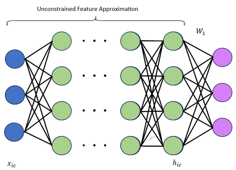
Figure 1: Illustration of the Unconstrained Feature Model in the case of a fully connected network.

3 The Deep Unconstrained Feature Model and DNC

The original unconstrained feature model (UFM) was introduced in [27]. We decompose similar to what was described in section 2.1, but we use an approximation for the component $h(x;\bar{\theta})$ of our network. Specifically, we make an approximation that this portion of the network is capable of mapping the training data to arbitrary points in feature space, treating the variables $h_{ic}$ as freely optimised variables. This is shown in Figure 1. Hence our set of parameters is now $(W_{L},b_{L},\{h_{ic}\})$. Since the other layers are hidden in the approximation, we consider $L$ to take the value 1 here.

This approximation means our network is only defined on the set of training data, and so we lose the ability to consider generalisation within this approximation. In addition the data dependence is removed from the model. The benefit of such a model is that it approximates the ability of modern deep learning networks to be highly expressive and allows for analysis at or near convergence.

Here we will consider the case where the loss function is MSE with L2 regularisation. We will also set the biases to zero. Choosing to write $H_{1}$ for the matrix of feature vectors, $H_{1}=[h_{1,1},...,h_{n,1},h_{1,2},...,h_{n,K}]\in\textbf{R}^{d_{L-1}\times Kn}$, our optimisation problem is now to minimise the following:

$$L(H_{1},W_{1})=\frac{1}{2Kn}\|W_{1}H_{1}-Y\|_{F}^{2}+\frac{1}{2}\lambda_{W_{1}}\|W_{1}\|_{F}^{2}+\frac{1}{2}\lambda_{H_{1}}\|H_{1}\|_{F}^{2},$$

where $Y=I_{K}\otimes 1_{n}^{T}$, with $1_{n}$ being the $n$ dimensional vector of 1’s, and $\lambda_{W_{1}},\lambda_{H_{1}}>0$ being regularisation parameters. $\otimes$ is the Kronecker product, specifically if $A\in\textbf{R}^{p_{1}\times q_{1}},B\in\textbf{R}^{p_{2}\times q_{2}}$ then

$$(A\otimes B)_{p_{2}(x-1)+y,q_{2}(u-1)+v}=A_{xu}B_{yv}.$$

Note this form of regularisation is different to what is used in a full DNN, since due to the approximation we must put the weight decay on $H_{1}$. Zhou et al. [31] have argued this is reasonable since the norm of $H_{1}$ is implicitly penalising the norm of $\bar{\theta}$.

Theoretical results have shown that, in the case of MSE loss, NC takes a stronger form [30]. The class means before global centering form an orthogonal frame, meaning that they are orthogonal vectors each of the same length. Note any orthogonal frame after global centering will form a simplex ETF, so the original NC property is implied by this stronger statement.

3.1 The L-Deep UFM

The UFM separates a single layer from the approximation. A natural extension is to consider separating multiple layers. This was originally considered by Tirer et al. [30] for the case of 2 separated layers with ReLU activation, Where it was shown that, subject to a technical constraint, the final layer will still demonstrate NC. Sukenik et al. [29] Worked with $L$ layers separated and managed to show collapse occurs at a layer-wise level, albeit only for the case $K=2$. In particular, the generalisation of NC3 they found was that the rows of the weight matrices are co-linear with one of the columns of the class means matrix of the previous layer features. In addition, both these works make clear the importance of regularisation in determining if DNC occurs. Too much regularisation leads to all parameters trivially being zero, yet non-zero amounts are required for collapse.

Choosing to separate $L$ layers, and taking $d_{L-1}=...=d_{1}=d$ for simplicity, our optimisation variables are $W_{L}\in\textbf{R}^{K\times d}$, $W_{L-1},...,W_{1}\in\textbf{R}^{d\times d}$, $H_{1}\in\textbf{R}^{d\times Kn}$, and our optimisation problem becomes to minimise the following:

$$L(H_{1},W_{1},...,W_{L})=\frac{1}{2Kn}\|W_{L}\sigma(W_{L-1}\sigma(...W_{2}\sigma(W_{1}H_{1})...))-Y\|_{F}^{2}+\sum_{l=1}^{L}\frac{1}{2}\lambda_{W_{l}}\|W_{l}\|_{F}^{2}+\frac{1}{2}\lambda_{H_{1}}\|H_{1}\|_{F}^{2},$$

where again $\lambda_{H_{1}},\lambda_{W_{1}},...,\lambda_{W_{L}}>0$ are regularisation parameters.

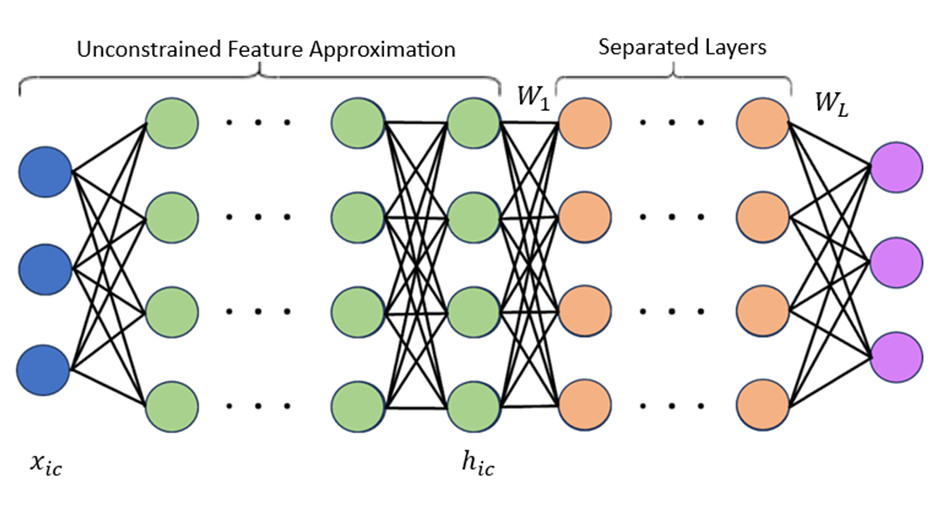
Figure 2: Illustration of the Deep Unconstrained Feature Model, separated layers either having ReLU or identity activation’s.

3.2 DNC in the L-Deep Linear UFM

The case where outside of the approximation $\sigma$ is set to identity was considered by Tirer et al. [30] for the bias-free MSE $L=2$ case, and Dang et al. [28] for both MSE and CE loss functions. In this case our optimisation objective is now:

$$L(H_{1},W_{1},...,W_{L})=\frac{1}{2Kn}\|W_{L}W_{L-1}...W_{1}H_{1}-Y\|_{F}^{2}+\sum_{l=1}^{L}\frac{1}{2}\lambda_{W_{l}}\|W_{l}\|_{F}^{2}+\frac{1}{2}\lambda_{H_{1}}\|H_{1}\|_{F}^{2}.$$ (1)

Dang et al. [28] provide a particularly complete description of DNC in the deep linear UFM. The results necessary from this work are stated below, which come from theorem 3.1 in their work:

Theorem 3.1 (from theorem 3.1 in [28]): Consider the deep linear UFM described in (1). Let $d\geq K$, and assume the level of regularisation is such that

$$\sqrt[L]{Kn\lambda_{W_{L}}\lambda_{W_{L-1}}...\lambda_{W_{1}}\lambda_{H_{1}}}<\frac{1}{KL^{2}}(L-1)^{\frac{L-1}{L}}.$$ (2)

Let $(W_{L}^{*},W_{L-1}^{*},...,W_{1}^{*},H_{1}^{*})$ be a global optimiser of (1), then we have the following results:

(DNC1): $H_{1}^{*}=\bar{H}^{*}\bigotimes 1_{n}^{T}$, where $\bar{H}^{*}=[\mu_{1},...,\mu_{K}]\in\textbf{R}^{d\times K}$.

(DNC2): $\forall l=1,...,L:$

$$W_{L}^{*}W_{L}^{*T}\propto\bar{H}^{*T}\bar{H}^{*}\propto W_{L}^{*}W_{L-1}^{*}...\bar{H}^{*}$$

$$\propto(W_{L}^{*}W_{L-1}^{*}...W_{l}^{*})(W_{L}^{*}W_{L-1}^{*}...W_{l}^{*})^{T}\propto I_{K}.$$

(DNC3): $\forall l=1,...,L:$

$$W_{L}^{*}W_{L-1}^{*}...W_{1}^{*}\propto\bar{H}^{*T},$$

$$W_{L}^{*}W_{L-1}^{*}...W_{l}^{*}\propto(W^{*}_{l-1}...W_{1}^{*}\bar{H}^{*})^{T}.$$

4 Low Dimensional Structure in the L-Deep Linear UFM

We can now consider how the observed low dimensional structure in deep learning models arises in the Deep Linear UFM. Due to the unconstrained features approximation we do not have access to the weights from the initial portion of the network. However, we can still consider layer-wise Hessians and layer-wise gradients for the separated layers, and as previously mentioned these have the same structure as the full Hessian and gradient. The unconstrained feature assumption allows us to consider the overparamatrisation limit, providing the limiting behaviour of these previously observed phenomena. We also include in Appendix E results for the other deep learning matrices considered by Papyan [10].

The assumption of linear activations in the final layer is made due to the technical difficulties of working with the full Deep UFM. We will explore the impact of this assumption in the next section.

First it will be helpful to define the following quantities for $1\leq l\leq L$:

$$A^{(l)}=W_{L}W_{L-1}...W_{l},$$

$$h_{ic}^{(l)}=W_{l-1}...W_{1}h_{ic},$$

$$\mu_{c}^{(l)}=\textrm{Av}_{i}\{h_{ic}^{(l)}\},$$

$$\mu_{G}^{(l)}=\textrm{Av}_{c}\{\mu_{c}^{(l)}\},$$

$$\bar{H}^{(l)}=[\mu_{1}^{(l)},...,\mu_{K}^{(l)}].$$

In addition note the MSE loss for a given sample is given by:

$$l(f(x_{ic};\theta),y_{c})=\frac{1}{2}\|W_{L}...W_{1}h_{ic}-y_{c}\|_{2}^{2}.$$

4.1 Hessian Spectra

We consider the layer-wise Hessian, which in the deep linear UFM is given by:

$$\textrm{Hess}_{l}=\textrm{Av}_{ic}\bigg{\{}\frac{\partial^{2}l(f(x_{ic};\theta),y_{c})}{\partial w_{l}^{2}}\bigg{\}},$$

where $w_{l}\in\textbf{R}^{d^{2}}$ are the weights from layer $l$ flattened into a vector in the standard way:

$$(w_{l})_{(d-1)x+y}=(W_{l})_{xy}.$$

Note we ignore the regularisation terms in this definition since they simply perturb the eigenvalues and leave the eigenvectors unchanged. Computing the derivatives and flattening, we recover the following Kronecker structure in the layer-wise Hessian:

$$\textrm{Hess}_{l}=A^{(l+1)T}A^{(l+1)}\otimes\Big{[}\textrm{Av}_{ic}\Big{\{}h_{ic}^{(l)}h_{ic}^{(l)T}\Big{\}}\Big{]}.$$

The full derivation is included in Appendix A. Note Kronecker structure has been previously observed in the Hessian [10, 46].

Using this structure and the properties of DNC, we have the following theorem about the layer-wise Hessian spectra at convergence:

Theorem 4.1: Consider the deep linear UFM described in (1). Let $d\geq K$, and assume the regularisation condition (2) holds. Let $(W_{L}^{*},...,W_{1}^{*},H_{1}^{*})$ be a global optima, then the rank of $\textrm{Hess}_{l}(W_{L}^{*},...,W_{1}^{*},H_{1}^{*})$ is $K^{2}$. The (unnormalised) eigenvectors corresponding to non-zero eigenvalues are given by:

$$\mu_{c}^{(l+1)}\otimes\mu_{c^{\prime}}^{(l)},\textrm{ for }c,c^{\prime}\in\{1,...,K\}.$$

In addition all the non-zero eigenvalues are equal, and have value: $\alpha^{(l+1)2}\|\mu_{c}^{(l+1)}\|^{2}_{2}\|\mu_{c^{\prime}}^{(l)}\|_{2}^{2}/K$, where $\alpha^{(l+1)}$ is the scaling constant between $A^{(l+1)T}$ and $\bar{H}^{(l+1)}$ at the optima.

We observe that the number of outlier eigenvalues seen in the Hessian’s of modern DNNs is recovered in the Deep Linear UFM. However, in this model, all nonzero eigenvalues are equal, whereas in DNNs it has been noted that they often have different values, with the largest $K$ being separated from the remaining $K(K-1)$ minibulk. This discrepancy could either be caused by the unconstrained feature approximation, or the use of linear layers instead of traditional ReLU layers. If it is due to the former, then it is likely this result signals the behaviour in the overparamatrization limit, and so points to the behaviour modern DNNs are tending to. In section 5 we will empirically investigate the cause of this discrepancy.

Crucially, we observe that the nonzero eigenvectors are constructs of the feature means, which characterise the DNC phenomenon. This elucidates why the class number frequently emerges in the observations of Hessian spectra. In the Linear Deep UFM, the intuitive phenomena of mapping data points from the same class to the same point and ensuring the separation of these points, coupled with the Kronecker structure of the layer-wise Hessian, necessarily results in the low dimensional structure of the eigenspace.

We can also examine Papyan’s decomposition in this model to explore how the cross-class structure is responsible for the outlier structure. First note that the analogy to the Gauss-Newton decomposition in this model is given by:

$$\textrm{Hess}_{l}=\textrm{Av}_{ic}\bigg{\{}\frac{\partial f(x_{ic};\theta)}{\partial w_{l}}\frac{\partial^{2}l(z,y_{c})}{\partial z^{2}}\Big{|}_{z=z_{ic}}\frac{\partial f(x_{ic};\theta)}{\partial w_{l}}\bigg{\}}+\textrm{Av}_{ic}\bigg{\{}\sum_{c^{\prime}}\frac{\partial l(z,y_{c})}{\partial z_{c^{\prime}}}\Big{|}_{z_{ic}}\frac{\partial^{2}f_{c^{\prime}}(x_{ic};\theta)}{\partial w_{l}^{2}}\bigg{\}},$$

where in our case $f(x_{ic};\theta)=W_{L}...W_{1}h_{ic}$, and as before $z_{ic}=f(x_{ic};\theta)$.

Here we will denote the pieces $G_{l}$ and $E_{l}$. Note that in the case of a piece wise linear activation function on MSE loss we have $\frac{\partial^{2}f_{c^{\prime}}(x_{ic};\theta)}{\partial w_{l}^{2}}=0$, so in our case $E_{l}=0$ and doesn’t contribute to the outliers of the spectrum, similar to what Papyan reports numerically. In addition for the MSE loss, $\frac{\partial^{2}l(z,y_{c})}{\partial z^{2}}|_{z=z_{ic}}=I$.

Papyan considered the CE loss, whereas here we work with the MSE loss. As a consequence we get a slightly different form for our $G_{l}$ matrix, but still with cross-class structure:

$$G_{l}=\sum_{i,c,c^{\prime}}\frac{1}{Kn}v_{icc^{\prime}}v_{icc^{\prime}}^{T},$$

where $v_{icc^{\prime}}=a_{c^{\prime}}^{(l+1)}\otimes h_{ic}^{(l)}$, and $(a_{c^{\prime}}^{(l+1)})_{x}=A_{c^{\prime}x}^{(l+1)}$, i.e. $a_{c^{\prime}}^{(l+1)}$ is the $c^{\prime}$th row of $A^{(l+1)}$. The full derivation is given in Appendix B. We can then decompose in a similar fashion to Papyan:

$$G_{l}=G_{l,\textrm{class}}+G_{l,\textrm{cross}}+G_{l,\textrm{within}},$$ (3)

where here we do not decompose the $G_{c=c^{\prime}}$ term, since it is not close to zero at an optima in the case of the MSE loss.

Considering these matrices at global optimum, we have the following theorem:

Theorem 4.2: Consider the deep linear UFM described in (1). Let $d\geq K$, and assume the regularisation condition (2) holds. Let $(W_{L}^{*},...,W_{1}^{*},H_{1}^{*})$ be a global optima, then the components in the decomposition described in (3), evaluated at this global optima, satisfy the following:

(a) $G_{l,\textrm{within}}=0$.

(b) $G_{l,\textrm{cross}}$ has rank $K(K-1)$, with one choice of spanning eigenvectors with non-zero eigenvalue given by

$$(\mu_{1}^{(l+1)}-\mu_{c^{\prime}}^{(l+1)})\otimes\mu_{c}^{l},\textrm{ for }c^{\prime}\in\{2,...,K\},c\in\{1,...,K\}.$$

(c) $G_{l,\textrm{class}}$ has rank $K$, with eigenvectors with non-zero corresponding eigenvalue given by

$$\mu_{G}^{(l+1)}\otimes\mu_{c}^{(l)},\textrm{ for }c\in\{1,...,K\}.$$

All non-zero eigenvalues are equal to $\alpha^{(l+1)2}\|\mu_{c}^{(l+1)}\|^{2}_{2}\|\mu_{c^{\prime}}^{(l)}\|_{2}^{2}/K$, where $\alpha^{(l+1)}$ is the scaling constant between $A^{(l+1)}$ and $\bar{H}^{(l)}$ at the optima. In addition the images of $G_{l,\textrm{class}}$, $G_{l,\textrm{cross}}$ are orthogonal spaces.

We observe that the structure in the decomposition described by Papyan [10] is recoverable in this model. The two matrices in the decomposition that contribute have the correct number of eigenvalues, and they project onto orthogonal spaces. Hence, when performing knockout, we exactly remove components of the image, perfectly lowering the rank of $\textrm{Hess}_{l}$, which explains the knockout results described by Papyan [10]. We also see that again the mean vectors of the layer-wise features are present in the structure. Note that as before the eigenvalues here are all equal, as opposed to seperating into a ’minibulk’ and a set of $K$ outliers. Again we will consider this in the next section.

4.2 Gradient Alignment with Outlier Eigenspace

We can also look at how the layer-wise gradients compare to the eigenvectors of the layer-wise Hessian. Now taking derivatives of the loss function including the regularisation terms, we have:

$$\frac{\partial L}{\partial(W_{l})_{ab}}=\lambda_{W_{l}}(W_{l})_{ab}+\textrm{Av}_{ic}\{(A^{(l+1)T}u_{ic})_{a}(h_{ic}^{(l)})_{b}\},$$

where we have defined $u_{ic}=W_{L}...W_{1}h_{ic}-y_{c}$. After flattening the weight vector similar to previously, we have:

$$g^{(l)}=\frac{\partial L}{\partial w^{(l)}}=\lambda_{W_{l}}w^{(l)}+\textrm{Av}_{ic}\{(A^{(l+1)T}u_{ic})\otimes h_{ic}^{(l)}\}.$$

To consider whether the gradient lies in the top eigenspace, we consider the second term in the above, which we call $\tilde{g}^{(l)}$, since this is the update to the weights. More details are given in Appendix C. We have the following theorem describing this term at the global optima.

theorem 4.3: Consider the deep linear UFM described in (1). Let $d\geq K$, and assume the regularisation condition (2) holds. Let $(W_{L}^{*},...,W_{1}^{*},H_{1}^{*})$ be a global optima. At this minima, we have

$$\tilde{g}^{(l)}=\frac{\beta^{(l+1)}}{K}\sum_{c=1}^{K}(\mu_{c}^{(l+1)}\otimes\mu_{c}^{(l)}),$$

where $\beta^{(l+1)}$ is a constant that can be expressed in terms of $\alpha^{(l+1)}$. Hence $\tilde{g}^{(l)}$ has exactly $K$ equal non-zero coefficients when expanded in the natural basis described in theorem 4.1.

Although in our model there are $K^{2}$ eigenvectors with non-zero eigenvalue, the layer-wise gradient update only has components corresponding to $K$ of these when written in the natural basis. This corresponds with the empirical observations of Gur-Ari et al. [17]. We also observe again that the feature mean structure induced by DNC is arising as further structure in the layer-wise gradients. However, since the $K^{2}$ non-zero eigenvalues are all equal, this term actually is an eigenvector of the Hessian exactly. Again, we can explore the full deep UFM model numerically to see if this specific peculiarity is induced by the choice of linear activation functions or the unconstrained feature approximation.

4.3 Weight Matrices

We can also consider the eigenspectra of the weight matrices at global optima. Specifically we consider the symmetric matrix $W_{l}^{T}W_{l}$ for each $l\in\{1,...,L\}$. We have the following theorem describing the eigenvalues

theorem 4.4: Consider the deep linear UFM described in (1). Let $d\geq K$, and assume the regularisation condition (2) holds. Let $(W_{L}^{*},...,W_{1}^{*},H_{1}^{*})$ be a global optima, then the matrices $W_{l}^{*}$ satisfy the following relation:

$$\lambda_{W_{l}}W_{l}^{*T}W_{l}^{*}=\lambda_{W_{l-1}}W_{l-1}^{*}W_{l-1}^{*T},$$

$$\lambda_{W_{1}}W_{1}^{*T}W_{1}^{*}=\lambda_{H_{1}}H_{1}^{*}H_{1}^{*T}.$$

As a consequence the rank of $W_{l}^{*T}W_{l}^{*}$ is $K$, and the non-zero eigenvalues are given by $\frac{\lambda_{H_{1}}}{\lambda_{W_{1}}}n\|\mu_{c}\|_{2}^{2}$ for $c\in\{1,...,K\}$.

More details are given in Appendix D. Note this again agrees with the number of outliers Papyan [10] observed, though again with equality.

5 Numerical Experiments

In this section, we empirically demonstrate our theoretical results for the deep linear UFM. In particular, we observe how the eigenvalues of the Hessian, gradients and weight matrices evolve over training. We will also consider how the theorems of section 5 carry over to the full deep UFM. Numerical results for the other deep learning matrices considered by Papyan [10], as well as further experiments for the deep UFM, are included in Appendix G.

5.1 Deep Linear UFM

For these experiments we use normally distributed weights as our initialisation, and set the following parameters: $K=3$, $d=60$, $n=40$, $L=5$, and consider the third layer $l=3$. The model is trained using gradient descent. In addition we kept track of the following DNC1 metric throughout training:

$$m=\|\Sigma_{W}^{(l)}\Sigma_{B}^{(l)\dagger}\|_{F}^{2},$$

where $\Sigma_{W}^{(l)},\Sigma_{B}^{(l)}$ are the within and between class variability at the layer $l$:

$$\Sigma_{W}^{(l)}=\frac{1}{Kn}\sum_{c=1}^{K}\sum_{i=1}^{n}(h_{ic}^{(l)}-\mu_{c}^{(l)})(h_{ic}^{(l)}-\mu_{c}^{(l)})^{T}$$

$$\Sigma_{B}^{(l)}=\frac{1}{K}\sum_{c=1}^{K}(\mu_{c}^{(l)}-\mu_{G}^{(l)})(\mu_{c}^{(l)}-\mu_{G}^{(l)})^{T}$$

and $\dagger$ denotes the Moore-Penrose pseudo-inverse operator. This intuitively captures that the class means should be separated, and shouldn’t collapse to the global mean $\mu_{G}^{(l)}$.

Considering this metric is important to ensure that the means remain separated and that our level of regularisation is not so large as to cause all weights to take value zero. In particular, [29] reported in their experiments with the deep UFM that the model can get stuck in saddle points when $d$ is set too small. We ensure this doesn’t occur in any of the following experiments.

Hessian Results

Figure 3 shows the bulk of the eigenvalues, along with the top $K^{2}=9$ outliers, at several stages of training. Initially all eigenvalues are close to zero, but very quickly the $K^{2}$ outliers seperate, and over a larger time scale they converge to the same value. This agrees with the results of theorem 4.1.

In addition, we can test how the predicted eigenvectors transform under $\textrm{Hess}_{l}$. Specifically, to measure the extent to which they are eigenvectors, we consider the following quantity:

$$f_{cc^{\prime}}=\frac{|(\mu_{c}^{(l+1)}\otimes\mu_{c^{\prime}}^{(l)})^{T}\textrm{Hess}_{l}(\mu_{c}^{(l+1)}\otimes\mu_{c^{\prime}}^{(l)})|^{2}}{\|(\mu_{c}^{(l+1)}\otimes\mu_{c^{\prime}}^{(l)})\|_{2}^{2}\|\textrm{Hess}_{l}(\mu_{c}^{(l+1)}\otimes\mu_{c^{\prime}}^{(l)})\|_{2}^{2}},$$

$f_{cc^{\prime}}$ measures the extent to which $\textrm{Hess}_{l}(\mu_{c}^{(l+1)}\otimes\mu_{c^{\prime}}^{(l)})$ aligns with $(\mu_{c}^{(l+1)}\otimes\mu_{c^{\prime}}^{(l)})$, and takes value 1 when $(\mu_{c}^{(l+1)}\otimes\mu_{c^{\prime}}^{(l)})$ is an eigenvector of $\textrm{Hess}_{l}$. Figure 4 shows this quantity for each of the $K^{2}$ predicted eigenvectors with non-zero eigenvalue over the early stages of training. We see each of these initially is far from being an eigenvector, but over training the alignment values $f_{cc^{\prime}}$ quickly get close to 1. Over further training these values converge to 1.

We can also consider how the decomposition results of theorem 4.2 arise. Figure 5 and Figure 6 show the outlier eigenvalues for $\textrm{Hess}_{l}$ as well as the knockouts of each component in the decomposition (3). We see that Knocking out $G_{l,\textrm{within}}$ has no effect on the spectrum, and knocking out $G_{l,\textrm{cross}}$, $G_{l,\textrm{class}}$ knocks out $K=3$, and $K(K-1)=6$ outlier eigenvalues respectively, as was stated in theorem 4.2.

Gradient Results

To test theorem 4.3, we can consider the coefficients of $\tilde{g}^{(l)}$ in an expansion in the natural basis $\mu_{c}^{(l+1)}\otimes\mu_{c^{\prime}}^{(l)}$.

$$\tilde{f}_{cc^{\prime}}=\frac{|(\mu_{c}^{(l+1)}\otimes\mu_{c^{\prime}}^{(l)})^{T}\tilde{g}^{(l)}|^{2}}{\|\mu_{c}^{(l+1)}\otimes\mu_{c^{\prime}}^{(l)}\|_{2}^{2}\|\tilde{g}^{(l)}\|_{2}^{2}}.$$

Figure 7 shows these quantities for each of the $K^{2}$ predicted eigenvectors with non-zero eigenvalue over the early stages of training. We see that quickly during training $K$ of these eigenvectors have non-zero coefficient, whereas the remaining have a coefficient of zero. Over further training these three non-zero coefficients converge to $1/K$, as is predicted by theorem 4.3.

Weight Results

Finally we can consider the eigenspectrum of the weight matrices $W_{l}^{T}W_{l}$. Figure 8 shows the bulk along with the top $K=3$ separated outliers. We see that similar to the Hessian the top eigenvalues initially are not well separated from the bulk, but over the course of training start to seperate, and with long timescales converge to the same value.

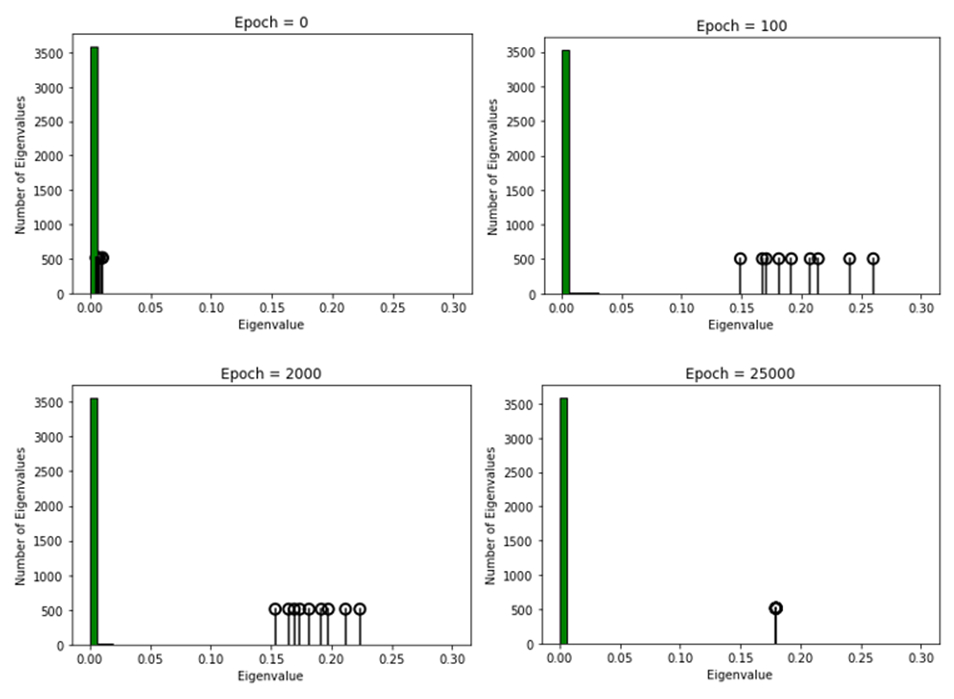
Figure 3: Histogram of the eigenvalues of $\textrm{Hess}_{l}$ for the Deep Linear UFM at an intermediate layer, with the top $K^{2}=9$ outliers plotted separately, for a range of training epochs. We see initially in training all eigenvalues are small, but as training progresses the top $K^{2}$ separate, and eventually take the same value.

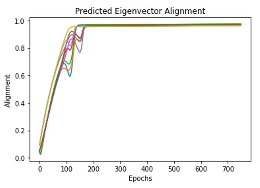
Figure 4: Plot of the quantities $f_{cc^{\prime}}$ over the early stages of training, showing the extent to which the predicted eigenvectors $(\mu_{c}^{(l+1)}\otimes\mu_{c^{\prime}}^{(l)})$ are eigenvectors of $\textrm{Hess}_{l}$. We see initially the predicted quantities are not eigenvectors of the Hessian, but throughout training they become eigenvectors. Note further training has all these alignments tend to 1.

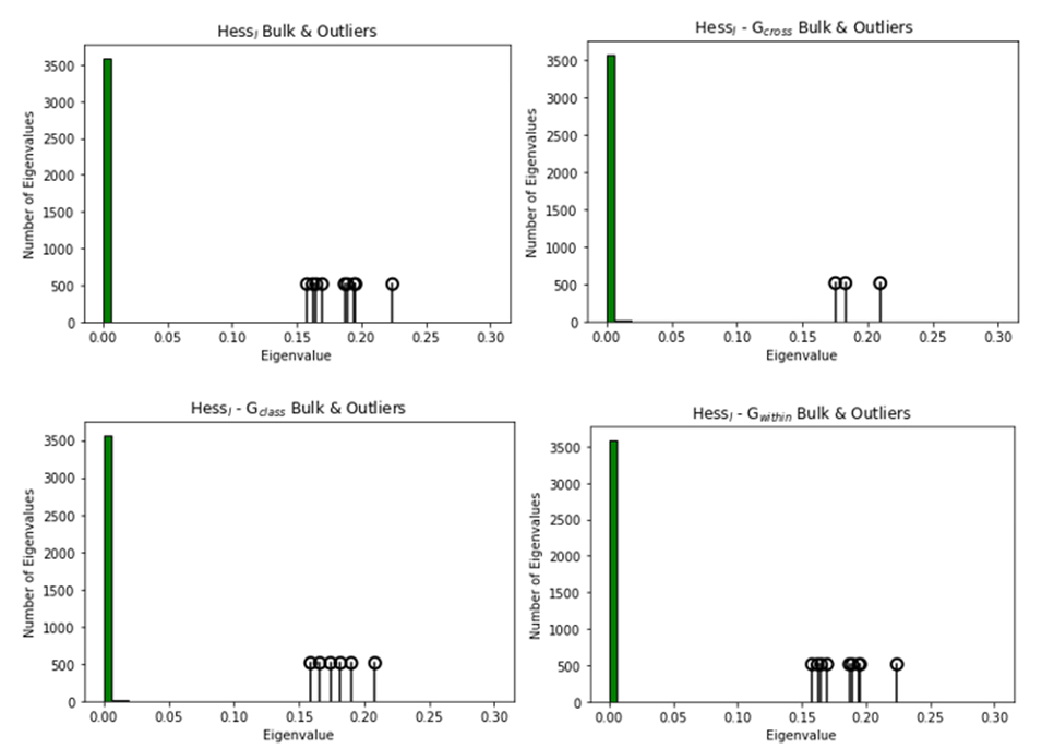
Figure 5: Histogram of the eigenvalues of $\textrm{Hess}_{l}$ for the Deep Linear UFM for an intermediate layer, with the top $K^{2}=9$ outliers plotted separately, after 2000 epochs, as well as knockouts of the decomposition described in (3). We see that knocking out each component has the predicted effect on the number of outlier eigenvalues.

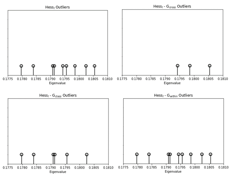
Figure 6: Plot of the top $K^{2}=9$ eigenvalues of $\textrm{Hess}_{l}$ for the Deep Linear UFM, after 25000 epochs, as well as knockouts of the decomposition described in (3). We see that knocking out each component has the predicted effect on the number of outlier eigenvalues.

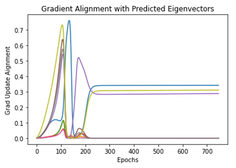
Figure 7: alignment coefficients of $\tilde{g}^{l}$ with the predicted eigenvectors described in theorem 4.1, for the Deep Linear UFM. We see that only $K$ of the $K^{2}$ eigenvectors with non-zero eigenvalue have non-zero component in the limit, and these are all roughly equal. Further training leads to each coefficient tending to $1/K$.

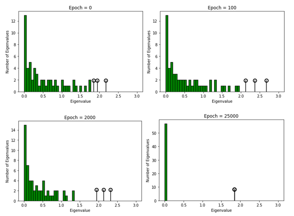
Figure 8: Histogram of the eigenvalues of $W_{l}^{T}W_{l}$ for the Deep Linear UFM at an intermediate layer, with the top $K=3$ outliers plotted separately, for a range of training epochs. We see initially in training the top outliers are not seperated from the others, but as training progresses the top $K$ separate, and eventually take the same value.

5.2 The Deep UFM

We can now consider how the results of the previous theorems extend over to the full deep UFM with ReLU activation’s on the separated layers. Note Sukenik et al. [29] showed that when $K=2$ we do not necessarily see DNC properties on the earliest layers outside of the approximation, so it is important to take $l\geq 3$ in this section. In addition, there is evidence that neural collapse occurs more in the later layers outside of the approximation, for this reason we focus on $l=4$. We also set $d=65$, with the other parameters remaining unchanged. We keep track of the DNC1 metric throughout these experiments also. Analytic expressions for the objects considered in this section can be found in Appendix F.

Hessian Results

Figure 9 shows the bulk and outlier eigenvalues of $\textrm{Hess}_{l}$ for a range of training epochs. Again initially all eigenvalues are close to zero, then the top $K^{2}$ outliers separate, and get closer to each other. Here however we do not see the values converge to equality. We see in figure 11 that in fact the weights do converge to equality, it is possible that with more training this will also occur with the Hessian. Indeed in the linear model we observed convergence for the weight eigenvalues significantly before the Hessian. It is therefore unclear whether the deep UFM will have identical structure to the deep linear UFM, or merely an approximation to it. We can also explore if the predicted eigenvectors carry over to the non-linear case. After $10^{6}$ training epochs, the coefficients $f_{cc^{\prime}}$ for the full Deep UFM took the values shown in Table 1. We see that these are significantly close to being eigenvectors, but again do not replicate the linear model results.

Figure 10 shows the Papyan decomposition in the case of the deep UFM. The knockout results do carry over, with the reduction in eigenvalue number matching the linear results and what Papyan reported empirically.

Gradient Results

In the non-linear case, since we did not see the predicted eigenvectors reach the point where they were true eigenvectors of $\textrm{Hess}_{l}$, we can not analyse the coefficients with a natural basis. Instead using the true eigenvectors of the layer-wise Hessian, after $10^{6}$ epochs, we get the values shown in Table 2 for the coefficients $\tilde{f}_{cc^{\prime}}$ with respects to the eigenvectors with non-zero eigenvalue of the deep UFM. only $K$ of the $K^{2}$ eigenvectors have non-zero component, but these are not all equal, as is predicted by the deep linear UFM results.

Weights

Figure 11 shows the weight eigenspectra at several stages of training. Surprisingly the outliers here do appear to converge to equality. Theoretical analysis is likely necessary to resolve this peculiarity.

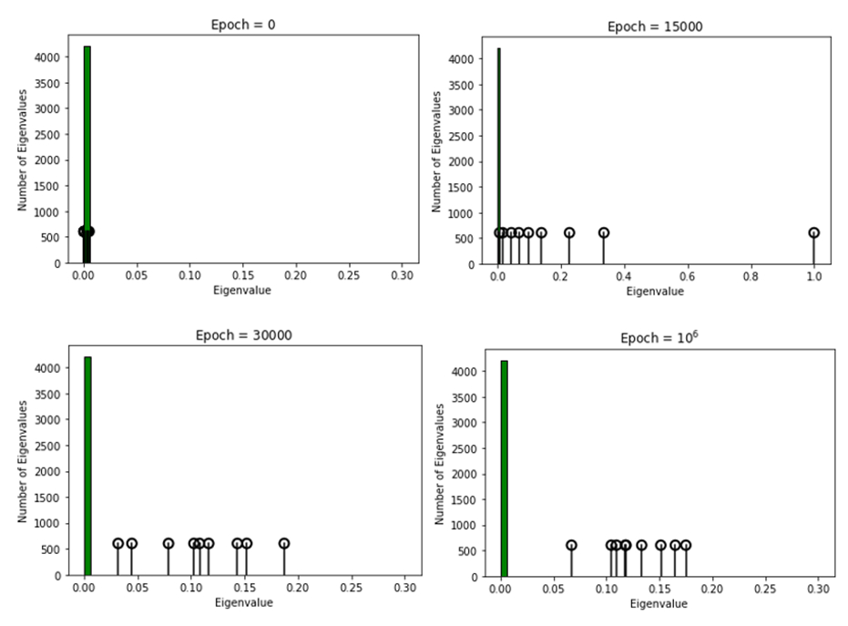
Figure 9: Histogram of the eigenvalues of $\textrm{Hess}_{l}$ for the Full Deep UFM at an intermediate layer, with the top $K^{2}=9$ outliers plotted separately, for a range of training epochs. We see initially in training the top outliers are not separated from the others, but as training progresses the top $K^{2}$ separate.

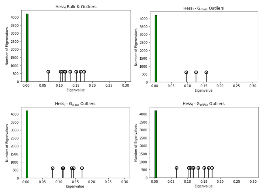
Figure 10: Histogram of the eigenvalues of $\textrm{Hess}_{l}$ for the Full Deep UFM at an intermediate layer, with the top $K^{2}=9$ outliers plotted separately, after $10^{6}$ training epochs, as well as the various knockouts. We see that knocking out each component has the predicted effect on the number of outlier eigenvalues.

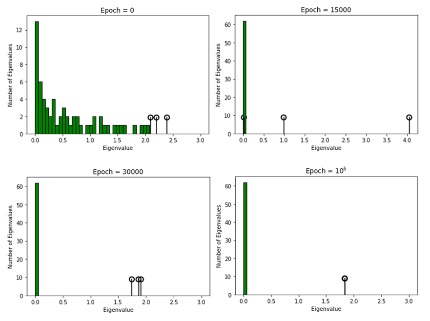
Figure 11: Histogram of the eigenvalues of $W_{l}^{T}W_{l}$ for the Full Deep UFM at an intermediate layer, with the top $K=3$ outliers plotted separately, for a range of training epochs. We see initially in training the top outliers are not seperated from the others, but as training progresses the top $K$ separate, and eventually take the same value.

6 Concluding Remarks

In this work we demonstrated that within the deep linear UFM with MSE loss, the low-dimensional observations of the Hessian spectra, gradients, and weight matrices are recoverable analytically. We showed that the structure induced by the DNC phenomenon leads to the other observed low dimensional structures and provided expressions for the eigenvectors and eigenvalues in terms of DNC quantities. This provides a justification for why the class number $K$ is so prevalent in the eigenspectra of matrices in deep learning. Moreover, we consider how analogies to these theoretical results arise in the full deep UFM, which provides insights into the convergence behaviour of highly overparamatrized neural networks.

In our work, we did not consider the full deep UFM theoretically, which would be the natural next step. At present, this has proved intractable to the wider research community. Whilst analysing DNNs has proven difficult, in the case of the unconstrained feature approximation the seperated layers do not increase the expressiveness of the function, and so it is possible this case will be more tractable. We leave it as further work to explore how DNC arises in the deep UFM, as well as the implications this has for eigenspectra of layer-wise matrices in this model. One possible analysis to resolve the numerical observations of section 5.2 would be to consider a perturbation to the identity activation, and expand to see if this causes the equality result to no longer hold. This would be potentially more tractable than dealing with the full deep UFM. There are also several simple extensions that we leave as further work, such as including biases or considering the CE loss function.

Table 1: values of the alignment coefficients $f_{cc^{\prime}}$ for the predicted eigenvectors from theorem 4.1, for the Deep UFM after $10^{6}$ training epochs.

Table 2: values of the coefficients $\tilde{f}_{cc^{\prime}}$ for the gradient with the true eigenvectors of $\textrm{Hess}_{l}$ for the Deep UFM after $10^{6}$ training epochs.

Appendices

A: Proof of Theorem 4.1

We begin by Proving the properties of the Hessian eigenvalues and eigenvectors in the deep linear UFM.

Recall our optimisation objective is:

$$L(H_{1},W_{1},...,W_{L})=\frac{1}{2Kn}\|W_{L}W_{L-1}...W_{1}H_{1}-Y\|_{F}^{2}+\sum_{l=1}^{L}\frac{1}{2}\lambda_{W_{l}}\|W_{l}\|_{F}^{2}+\frac{1}{2}\lambda_{H_{1}}\|H_{1}\|_{F}^{2}.$$

We consider the Hessian with respects to the parameters of a given layer $W_{l}$, and drop the regularisation terms since they just shift the spectrum. It is convenient to write our objective in terms of the individual training points, and define $u_{ic}=W_{L}...W_{1}h_{ic}-y_{c}$, so that:

$$L(H_{1},W_{1},...,W_{L})=\textrm{Av}_{ic}\bigg{\{}\frac{1}{2}\|W_{L}...W_{1}h_{ic}-y_{c}\|_{2}^{2}\bigg{\}}=\textrm{Av}_{ic}\bigg{\{}\frac{1}{2}u_{ic}^{T}u_{ic}\bigg{\}}.$$

Taking derivatives gives:

$$\frac{\partial^{2}L}{\partial(W_{l})_{ab}\partial(W_{l})_{ef}}=\textrm{Av}_{ic}\bigg{\{}\frac{\partial u_{ic}}{\partial(W_{l})_{ab}}\cdot\frac{\partial u_{ic}}{\partial(W_{l})_{ef}}\bigg{\}}+\textrm{Av}_{ic}\bigg{\{}\frac{\partial^{2}u_{ic}}{\partial(W_{l})_{ab}(W_{l})_{ef}}\cdot u_{ic}\bigg{\}}.$$

The second of these is zero for our linear case. Defining the quantities:

$$A^{(l+1)}=W_{L}...W_{l+1},$$

$$B^{(l-1)}=W_{l-1}...W_{1},$$

we get the following:

$$\frac{\partial^{2}L}{\partial(W_{l})_{ab}\partial(W_{l})_{ef}}=\textrm{Av}_{ic}\bigg{\{}\sum_{x}A^{(l+1)}_{xe}(B^{(l-1)}h_{ic})_{f}A^{(l+1)}_{xa}(B^{(l-1)}h_{ic})_{b}\bigg{\}}.$$

After defining $h_{ic}^{(l)}=W_{l-1}...W_{1}h_{ic}$, this becomes:

$$\frac{\partial^{2}L}{\partial(W_{l})_{ab}\partial(W_{l})_{ef}}=\textrm{Av}_{ic}\Big{\{}(A^{(l+1)T}A^{(l+1)})_{ae}(h_{ic}^{(l)})_{b}(h_{ic}^{(l)})_{f}\Big{\}}.$$

Now to write this as a $d^{2}\times d^{2}$ matrix, we flatten $W_{l}$ in the standard way:

$$(w_{l})_{(d-1)x+y}=(W_{l})_{xy},$$

and this gives:

$$\textrm{Hess}_{l}=\frac{\partial^{2}L}{\partial^{2}w_{l}}=A^{(l+1)T}A^{(l+1)}\otimes\Big{[}\textrm{Av}_{ic}\Big{\{}h_{ic}^{(l)}h_{ic}^{(l)T}\Big{\}}\Big{]}.$$

Here $\otimes$ is the Kronecker product, specifically if $A\in\textbf{R}^{p_{1}\times q_{1}},B\in\textbf{R}^{p_{2}\times q_{2}}$ then

$$(A\otimes B)_{p_{2}(x-1)+y,q_{2}(u-1)+v}=A_{xu}B_{yv}.$$

We now assume we are at a point of convergence, and so can use the properties of deep neural collapse shown in theorem 3.1 of [28]. Specifically, assuming the level of regularisation is not too large, in the sense that

$$K(Kn\lambda_{W_{L}}\lambda_{W_{L-1}}...\lambda_{W_{1}}\lambda_{H_{1}})^{\frac{1}{L}}<\frac{(L-1)^{\frac{L-1}{L}}}{L^{2}},$$

then we have the first deep neural collapse property: $h_{ic}=\mu_{c}$, where $\mu_{c}=\textrm{Av}_{ic}\{h_{ic}\}$. In addition defining $\mu_{c}^{(l)}=W_{l-1}...W_{1}\mu_{c}$, our Hessian is now:

$$\textrm{Hess}_{l}=A^{(l+1)T}A^{(l+1)}\otimes\Big{[}\textrm{Av}_{c}\Big{\{}\mu_{c}^{(l)}\mu_{c}^{(l)T}\Big{\}}\Big{]}.$$

Now assume $d\geq K$, and define the matrix of class means at the $l$th layer: $M^{(l)}=[\mu_{1}^{(l)},...,\mu_{K}^{(l)}]\in\textbf{R}^{d\times K}$. Note the following corollary:

Corollary A.1: assume the regularisation condition (2) is satisfied, and $d\geq K$. Then the columns of $M^{(l)}$ form an orthogonal frame in the sense that $M^{(l)T}M^{(l)}\propto I_{K}$ .

Proof: Note though this is not explicitly stated in theorem 3.1 of [28], it is an immediate consequence of DNC 2 and DNC3 in the theorem statement.

We can now consider the right side of our Kronecker product. The class means are orthogonal, and so the matrix $\frac{1}{K}\sum_{c=1}^{K}\mu_{c}^{(l)}\mu_{c}^{(l)T}$ has rank $K$ and is simply a scaled projection onto $\textrm{Span}\{\mu_{c}^{(l)}\}_{c=1}^{K}$ with eigenvectors $\hat{\mu}_{c}^{(l)}$. In addition since the class means have the same norm, the non-zero eigenvalues are all equal, with value $\|\mu_{c}^{(l)}\|_{2}^{2}/K$.

For the left side of our Kronecker product, note that from the third DNC property, we have $A^{(l+1)}\propto M^{(l+1)T}$, and so the rows $a_{c}^{(l+1)}$ of $A^{(l+1)}$ are such that $a_{c}^{(l+1)}=\alpha^{(l+1)}\mu_{c}^{(l+1)}$, for some constant $\alpha^{(l+1)}$. Since these are independent, the rank of $A^{(l+1)}$ is exactly $K$, and hence this is also the rank of $A^{(l+1)T}A^{(l+1)}$.

By considering $A^{(l+1)T}A^{(l+1)}$ acting on $\mu_{c}^{(l+1)}$, we see that the eigenvectors with non-zero eigenvalue are $\hat{\mu}_{c}^{(l+1)}$, and the corresponding eigenvalues are all equal to $\alpha^{(l+1)2}\|\mu_{c}^{(l+1)}\|_{2}^{2}$.

Hence as a consequence of the properties of the Kronecker product, our layer-wise Hessian $\textrm{Hess}_{l}$ has rank $K^{2}$, with eigenvectors $\hat{\mu}_{c}^{(l+1)}\otimes\hat{\mu}_{c}^{(l)}$ for $c,c^{\prime}\in\{1,...,K\}$, with corresponding eigenvalues $\alpha^{(l+1)2}\|\mu_{c}^{(l+1)}\|_{2}^{2}\|\mu_{c^{\prime}}^{(l)}\|_{2}^{2}/K.$

B: Proof of Theorem 4.2

We now look at the analogy to Papyan’s decomposition of the Fisher Information Matrix via cross-class structure. Much of the work in this section is similar to the previous, however we still present the details here to make clear how cross-class structure emerges in the layer-wise Hessian of the deep linear UFM similar to the empirical results of Papyan [10] for the CE loss.

define $l(a,b)=\frac{1}{2}\|a-b\|_{2}^{2}$ and the mapping of a datapoint under our approximation as: $f(x_{ic};\theta)=W_{L}...W_{1}h_{ic}$. Again ignoring regularisation terms, the Hessian at layer $l$ is:

$$\textrm{Hess}_{l}=\textrm{Av}_{ic}\bigg{\{}\frac{\partial^{2}l(f(x_{ic};\theta),y_{c})}{\partial w_{l}^{2}}\bigg{\}},$$

which we can use the Gauss-Newton decomposition to write as:

$$=\textrm{Av}_{ic}\bigg{\{}\frac{\partial f(x_{ic};\theta)}{\partial w_{l}}\frac{\partial^{2}l(z,y_{c})}{\partial z^{2}}\Big{|}_{z=z_{ic}}\frac{\partial f(x_{ic};\theta)}{\partial w_{l}}\bigg{\}}+\textrm{Av}_{ic}\bigg{\{}\sum_{c^{\prime}}\frac{\partial l(z,y_{c})}{\partial z_{c^{\prime}}}\Big{|}_{z_{ic}}\frac{\partial^{2}f_{c^{\prime}}(x_{ic};\theta)}{\partial w_{l}^{2}}\bigg{\}},$$

where $z_{ic}=f(x_{ic};\theta)$. Call the first of these $G_{l}$ and the second $E_{l}$. Papyan observed $E_{l}$ doesn’t contribute to the outliers of the spectrum of the Hessian. In our case, since $\frac{\partial^{2}f_{c^{\prime}}(x_{ic};\theta)}{\partial w_{l}^{2}}=0$ we have that $E=0$, and so $\textrm{Hess}_{l}=G_{l}$.

Papyan worked with CE loss and showed in the case of the full Hessian that $G=\sum_{i,c,c^{\prime}}w_{icc^{\prime}}g_{icc^{\prime}}g_{icc^{\prime}}^{T}$, where $g_{icc^{\prime}}=\frac{\partial l(f(x_{ic};\theta),y_{c^{\prime}})}{\partial\theta}\in\textbf{R}^{p}$ are the extended gradients, and $w_{icc^{\prime}}\in\textbf{R}$ are weights.

Since we are using the MSE loss, we get a slightly different decomposition. Noting that $\frac{\partial^{2}l(z,y_{c})}{\partial z^{2}}=I$, if we define the quantities:

$$v_{icc^{\prime}}=\frac{\partial f_{c^{\prime}}(x_{ic};\theta)}{\partial w_{l}},$$

we have:

$$G_{l}=\sum_{i,c,c^{\prime}}\frac{1}{Kn}v_{icc^{\prime}}v_{icc^{\prime}}^{T},$$

where $v_{icc^{\prime}}=a_{c^{\prime}}^{(l+1)}\otimes h_{ic}^{(l)}$, with $(a_{c^{\prime}}^{(l+1)})_{x}=A^{(l+1)}_{c^{\prime}x}$ being the rows of $A^{(l+1)}$ as before, and $A^{(l+1)}$, $h_{ic}^{(l)}$ defined previously. Note this is a weighted second moment matrix of the objects $v_{icc^{\prime}}$.

Papyan then decomposed the sum in $G$ into 4 distinct pieces:

$$G=G_{\textrm{within}}+G_{\textrm{cross}}+G_{\textrm{class}}+G_{c=c^{\prime}}.$$

The first two terms look at the covariance of his objects $g_{i,c,c}$ over the $i$ and $c^{\prime}$ indices respectively, whilst the third considers the second moment over the $c$ index. Papyan hypothesised that these covariances and second moment directly contribute the distinct components in the Hessian eigenspectra. The final term is an accumulation of terms from the others that take value zero at an optima.

In our case it does not make sense to separate out the $G_{c=c^{\prime}}$ term, since whilst for the CE loss this term is zero at an optima, it is not the case for our MSE decomposition. First defining the quantities:

$$v_{cc^{\prime}}=\sum_{i}\frac{1}{n}v_{icc^{\prime}},$$

$$v_{c}=\sum_{c^{\prime}}\frac{1}{K}v_{cc^{\prime}}.$$

Instead we decompose as:

$$G_{l}=G_{l,\textrm{class}}+G_{l,\textrm{cross}}+G_{l,\textrm{within}},$$

where the components of the decomposition are given by:

$$G_{l,\textrm{class}}=\sum_{c}v_{c}v_{c}^{T},$$

$$G_{l,\textrm{cross}}=\sum_{c}G_{l,\textrm{cross},c},$$

where

$$G_{l,\textrm{cross},c}=\sum_{c^{\prime}}\frac{1}{K}(v_{cc^{\prime}}-v_{c})(v_{cc^{\prime}}-v_{c})^{T},$$

and

$$G_{l,\textrm{within}}=\sum_{c,c^{\prime}}\frac{1}{K}G_{l,\textrm{within},c,c^{\prime}},$$

where:

$$G_{l,\textrm{within},c,c^{\prime}}=\sum_{i}\frac{1}{n}(v_{icc^{\prime}}-v_{cc^{\prime}})(v_{icc^{\prime}}-v_{cc^{\prime}})^{T}.$$

We can now again assume we are at a point of convergence and use properties of neural collapse. Again assuming the level of regularisation satisfies (2) and that $d\geq K$, the first NC property gives us that $h_{ic}=\mu_{c}$, and hence $v_{icc^{\prime}}=v_{cc^{\prime}}$. As a consequence $G_{l,\textrm{within}}=0$ and does not contribute to the outlier eigenvalues of the spectrum, which again agrees with the results of Papyan.

In addition using Corollary A.1, and theorem 3.1 from [28] gives us that $a_{c^{\prime}}^{(l+1)}=\alpha^{(l+1)}\mu_{c^{\prime}}^{(l+1)}$, for some constant $\alpha^{(l+1)}$. So at the optima we have:

$$v_{cc^{\prime}}=\alpha^{(l+1)}\mu_{c^{\prime}}^{(l+1)}\otimes\mu_{c}^{(l)},$$

as well as:

$$v_{c}=\frac{1}{K}\sum_{c^{\prime}}v_{cc^{\prime}}=\frac{1}{K}\sum_{c^{\prime}}\alpha^{(l+1)}\mu_{c^{\prime}}^{(l+1)}\otimes\mu_{c}^{(l)}=\alpha^{(l+1)}\mu_{G}^{(l+1)}\otimes\mu_{c}^{(l)},$$

$$v_{cc^{\prime}}-v_{c}=\alpha^{(l+1)}(\mu_{c^{\prime}}^{(l+1)}-\mu_{G}^{(l+1)})\otimes\mu_{c}^{(l)}.$$

So, the form of our decomposition components is given by:

$$G_{l,\textrm{class}}=\alpha^{(l+1)2}\sum_{c=1}^{K}(\mu_{G}^{(l+1)}\otimes\mu_{c}^{(l)})(\mu_{G}^{(l+1)}\otimes\mu_{c}^{(l)})^{T},$$

$$G_{l,\textrm{cross}}=\frac{\alpha^{(l+1)2}}{K}\sum_{c,c^{\prime}=1}^{K}([\mu_{c^{\prime}}^{(l+1)}-\mu_{G}^{(l+1)}]\otimes\mu_{c}^{(l)})([\mu_{c^{\prime}}^{(l+1)}-\mu_{G}^{(l+1)}]\otimes\mu_{c}^{(l)})^{T}.$$

Hence $G_{l,\textrm{class}}$ is simply a scaled projection operator onto $\textrm{Span}\{\mu_{G}^{(l+1)}\otimes\mu_{c}^{(l)}\}_{c=1}^{K}$, and so has rank $K$. Also note the eigenvalues are equal to what was reported in the previous appendix (since $\|\mu_{G}^{(l+1)}\|_{2}^{2}=\frac{1}{K}\|\mu_{c}^{(l+1)}\|_{2}^{2}$), with eigenvectors given by $\mu_{G}^{(l+1)}\otimes\mu_{c}^{(l)}$ for $c\in\{1,...,K\}$

Similarly $G_{l,\textrm{cross}}$ has image: $\textrm{Span}\{(\mu_{c^{\prime}}^{(l+1)}-\mu_{G}^{(l+1)})\otimes\mu_{c}^{(l)}\}_{c,c^{\prime}=1}^{K}$. The globally centred means $\mu_{c^{\prime}}^{(l+1)}-\mu_{G}^{(l+1)}$ are clearly not linearly independent, since they sum to zero, and so span a $K-1$ dimensional space (they in fact form a simplex ETF). As a consequence the rank of $G_{l,\textrm{cross}}$ is $K(K-1)$. It is easy to verify that one choice of spanning eigenvectors for the non-zero eigenvalues is given by $(\mu_{1}^{(l+1)}-\mu_{c^{\prime}}^{(l+1)})\otimes\mu_{c}^{(l)}$, for $c^{\prime}\in\{2,...,K\}$, $c\in\{1,...,K\}$ with eigenvalues the same as what was reported in the previous appendix.

It is also easy to see that the vectors in the two projections are orthogonal, and so $G_{l,\textrm{class}}$ and $G_{l,\textrm{cross}}$ knockout different parts of the projection in $\textrm{Hess}_{l}$, which is why we observe the spectrum results shown in Section 5 when doing subtraction knockout.

C: Proof of Theorem 4.3

we now consider the layer-wise gradient close to an optima, and show it approximately lies in the top eigenspace of the corresponding layer-wise Hessian. As before we have:

$$L=\textrm{Av}_{ic}\bigg{\{}\frac{1}{2}\|W_{L}...W_{1}h_{ic}-y_{c}\|_{2}^{2}\bigg{\}}+\frac{1}{2}\lambda_{W_{l}}\|W_{l}\|_{F}^{2}+....$$

Writing $u_{ic}=W_{L}...W_{1}h_{ic}-y_{c}$, the derivative is

$$\frac{\partial L}{\partial(W_{l})_{ab}}=\lambda_{W_{l}}(W_{l})_{ab}+\textrm{Av}_{ic}\bigg{\{}\sum_{x,y,z,u}(u_{ic})_{x}\frac{\partial}{\partial(W_{l})_{ab}}(A_{xy}^{(l+1)}(W_{l})_{yz}B_{zu}^{(l-1)}(h_{ic})_{u})\bigg{\}}$$

$$=\lambda_{W_{l}}(W_{l})_{ab}+\textrm{Av}_{ic}\Big{\{}\sum_{x,u}(u_{ic})_{x}A_{xa}^{(l+1)}B_{bu}^{(l-1)}(h_{ic})_{u}\Big{\}}$$

$$=\lambda_{W_{l}}(W_{l})_{ab}+\textrm{Av}_{ic}\Big{\{}(A^{(l+1)T}u_{ic})_{a}(h_{ic}^{(l)})_{b}\Big{\}}.$$

After flattening $W_{l}$, we have:

$$g^{(l)}=\frac{\partial L}{\partial w^{(l)}}=\lambda_{W_{l}}w^{(l)}+\textrm{Av}_{ic}\Big{\{}(A^{(l+1)T}u_{ic})\otimes h_{ic}^{(l)}\Big{\}}.$$

To show that the gradient lies in this top eigenspace, it is sufficient to show the second term in the above lies in this eigenspace at a minima, since this is the update to the weights. In particular Gur-Ari et al. [17] considered $g$ itself, whereas Ben Arous et al. [18] consider the weights. Since the top eigenspace is preserved when we are close to minima, as is seen in theorem 4.1, these two results coincide with considering the second term. So now consider $\tilde{g}^{(l)}=\textrm{Av}_{ic}\{(A^{(l+1)T}u_{ic})\otimes h_{ic}^{(l)}\}$.

Again assuming the regularisation condition (2) and $d\geq K$, the DNC1 property $h_{ic}=\mu_{c}$ reduces our quantity to:

$$\textrm{Av}_{ic}\Big{\{}(A^{(l+1)T}u_{ic})\otimes h_{ic}^{(l)}\Big{\}}=\textrm{Av}_{c}\Big{\{}(A^{(l+1)T}u_{c})\otimes\mu_{c}^{(l)}\Big{\}},$$

where we have defined the quantity: $u_{c}=W_{L}...W_{1}\mu_{c}-y_{c}$

We consider the left quantity in our Kronecker product separately. Recall from theorem 3.1 of [28] and Corollary A.1 that the rows $a_{c}^{(l+1)}$ of $A^{(l+1)}$ have the form $a_{c}^{(l+1)}=\alpha^{(l+1)}\mu_{c}^{(l+1)}$. Hence $A^{(l+1)T}=\alpha^{(l+1)}[\mu_{1}^{(l+1)}...\mu_{K}^{(l+1)}]$, and so $A^{(l+1)T}y_{c}=\alpha^{(l+1)}\mu_{c}^{(l+1)}$

Also

$$A^{(l+1)T}W_{L}...W_{1}\mu_{c}^{(1)}=A^{(l+1)T}A^{(l+1)}\mu_{c}^{(l+1)}.$$

Using the form of $A^{(l+1)}$ We find that

$$A^{(l+1)T}A^{(l+1)}\mu_{c}^{(l+1)}=\alpha^{(l+1)2}\|\mu_{c}^{(l+1)}\|_{2}^{2}\mu_{c}^{(l+1)},$$

and so:

$$A^{(l+1)T}u_{c}=\Big{[}\alpha^{(l+1)2}\|\mu_{c}^{(l+1)}\|_{2}^{2}-\alpha^{(l+1)}\Big{]}\mu_{c}^{(l+1)}.$$

Note this coefficient is non-zero, else the weights would be zero at the global optima, contradicting the properties of DNC. Defining the coefficient to be $\beta^{(l+1)}$, we have that:

$$\textrm{Av}_{ic}\Big{\{}A^{(l+1)T}u_{ic}\otimes h_{ic}^{(l)}\Big{\}}=\frac{\beta^{(l+1)}}{K}\sum_{c}(\mu_{c}^{(l+1)}\otimes\mu_{c}^{(l)}).$$

Now recall the set of (unnormalised) eigenvectors of the corresponding layer-wise Hessian at an optima are given by: $\{\mu_{c^{\prime}}^{(l+1)}\otimes\mu_{c}^{(l)}\}_{c,c^{\prime}=1}^{K}$. We see that with this basis the gradient lies in a $K$ dimensional subspace with equal coefficients for each.

Note there is a subtlety here, since all the non-zero eigenvalues are equal, a different choice of basis vectors leads to a different number of non-zero coefficients. However in this natural basis choice, we recover a similar result to Gur-Ari and Ben Arous.

D: Proof of Theorem 4.4

We can now consider the structure of the eigenspectrum of the weight matrices $W_{l}^{T}W_{l}$ at global optima. This proof for the most part arises in the proof of theorem 3.1 in [28], though we include the details for completeness. First note by setting derivatives of the loss equal to zero, we have the following set of equations:

$$\frac{\partial L}{\partial W_{l}}=\lambda_{W_{l}}W_{l}+\frac{1}{Kn}A^{(l+1)T}(W_{L}...W_{1}H_{1}-Y)(B^{(l-1)}H_{1})^{T}=0,\>\>\forall l\in\{1,...,L\},$$

$$\frac{\partial L}{\partial H_{1}}=\lambda_{H_{1}}H_{1}+\frac{1}{Kn}A^{(1)T}(W_{L}...W_{1}H_{1}-Y)=0.$$

Next by considering

$$W_{l}^{T}\frac{\partial L}{\partial W_{l}}-\frac{\partial L}{\partial W_{l-1}}W_{l-1}^{T}=0,$$

we have:

$$\lambda_{W_{l}}W_{l}^{T}W_{l}=\lambda_{W_{l-1}}W_{l-1}W_{l-1}^{T}.$$

Since $M^{T}M$ and $MM^{T}$ have the same non-zero eigenvalues, if ${s^{(l)}_{i}}$ are the set of eigenvalues of $W_{l}^{T}W_{l}$, then we have the following recurrence:

$$s^{(l)}_{i}=\frac{\lambda_{W_{l-1}}}{\lambda_{W_{l}}}s_{i}^{(l-1)},$$

And applying this iteratively we have:

$$s_{i}^{(l)}=\frac{\lambda_{W_{1}}}{\lambda_{W_{l}}}s_{i}^{(1)}.$$

We also have

$$W_{1}^{T}\frac{\partial L}{\partial W_{1}}-\frac{\partial L}{\partial H_{1}}H_{1}^{T}=0,$$

and so:

$$s_{i}^{(l)}=\frac{\lambda_{H_{1}}}{\lambda_{W_{l}}}\tilde{s}_{i},$$

Where $\{\tilde{s}_{i}\}$ are the eigenvalues of $H_{1}H_{1}^{T}$. Using the DNC results for $H_{1}$, we have that its columns are given by $n$ repeats of the mean vectors $\mu_{c}$, and so the non-zero eigenvalues of $H_{1}H_{1}^{T}$ are $n\|\mu_{c}\|_{2}^{2}$ for $c\in\{1,...,K\}$

Hence the non-zero eigenvalues of the Weight matrix $W_{l}^{T}W_{l}$ are given by $\frac{\lambda_{H_{1}}}{\lambda_{W_{l}}}n\|\mu_{c}\|_{2}^{2}$, for $c\in\{1,...,K\}$.

E: Other Deep Learning Matrices

E.1: Covariance of Gradients

We can also look at the covariance of gradients, which were considered empirically by [12]. Specifically, we look at the matrix:

$$C^{(l)}=\textrm{Av}_{ic}\big{\{}(g_{ic}^{(l)}-g^{(l)})(g_{ic}^{(l)}-g^{(l)})^{T}\big{\}},$$

where

$$g_{ic}^{(l)}=\nabla_{w^{(l)}}l(f(x_{ic};\theta),y_{c}),$$

$$g^{(l)}=\textrm{Av}_{ic}\big{\{}g_{ic}^{(l)}\big{\}}.$$

Note here we are only working with the gradient with respects to the MSE, not the full loss including the regularisers, and again work at a layer-wise level. Recall from Appendix C that:

$$\nabla_{w^{(l)}}l(f(x_{ic};\theta),y_{c})=A^{(l+1)T}u_{ic}\otimes h_{ic}^{(l)}.$$

Again assuming the regularisation condition (2) and $d\geq K$, we know from Appendix C that at optima we have:

$$A^{(l+1)T}u_{ic}=\beta^{(l+1)}\mu_{c}^{(l+1)},$$

and so

$$g_{ic}^{(l)}=\beta^{(l+1)}\mu_{c}^{(l+1)}\otimes\mu_{c}^{(l)},$$

$$g^{(l)}=\frac{\beta^{(l+1)}}{K}\sum_{c=1}^{K}\mu_{c}^{(l+1)}\otimes\mu_{c}^{(l)}.$$

Hence we can write $C^{(l)}$ at the optima as:

$$C^{(l)}=\frac{\beta^{(l+1)2}}{K}\sum_{c=1}^{K}\bigg{[}(\mu_{c}^{(l+1)}\otimes\mu_{c}^{(l)})-\textrm{Av}_{c^{\prime}}\Big{\{}\mu_{c^{\prime}}^{(l+1)}\otimes\mu_{c^{\prime}}^{(l)}\Big{\}}\bigg{]}\bigg{[}(\mu_{c}^{(l+1)}\otimes\mu_{c}^{(l)})-\textrm{Av}_{c^{\prime\prime}}\Big{\{}\mu_{c^{\prime\prime}}^{(l+1)}\otimes\mu_{c^{\prime\prime}}^{(l)}\Big{\}}\bigg{]}^{T}.$$

Note the vectors $\mu_{c}^{(l+1)}\otimes\mu_{c}^{(l)}$ are orthogonal, and so the vectors $(\mu_{c}^{(l+1)}\otimes\mu_{c}^{(l)})-\textrm{Av}_{c^{\prime}}\{\mu_{c^{\prime}}^{(l+1)}\otimes\mu_{c^{\prime}}^{(l)}\}$ form a simplex ETF. As a consequence they span a $K-1$ dimensional subspace. In addition it is simple to show that the matrix $C^{(l)}$ has eigenvectors with non-zero eigenvalue given by: $\mu_{1}^{(l+1)}\otimes\mu_{1}^{(l)}-\mu_{c}^{(l+1)}\otimes\mu_{c}^{(l)}$ for $c\in\{2,...,K\}$, each with eigenvalue $\beta^{(l+1)2}\|\mu_{c}^{(l+1)}\|_{2}^{2}\|\mu_{c}^{(l)}\|_{2}^{2}/K$. Thus we have the following theorem for the second moment of gradients:

Theorem E.1: Consider the deep linear UFM described in (1). Let $d\geq K$, and assume the regularisation condition (2) holds. Let $(W_{L}^{*},...,W_{1}^{*},H_{1}^{*})$ be a global optima, then the matrix $C^{(l)}$ at this optima has $K-1$ non-zero equal eigenvalues, taking value $\frac{\beta^{(l+1)2}}{K}\|\mu_{c}^{(l+1)}\|_{2}^{2}\|\mu_{c}^{(l)}\|_{2}^{2}$, with one set of spanning (unnormalised) eigenvectors being $(\mu_{1}^{(l+1)}\otimes\mu_{1}^{(l)}-\mu_{c}^{(l+1)}\otimes\mu_{c}^{(l)})$ for $c\in\{2,...,K\}$.

Jastrzębski et al. [12] reported a bulk-outlier structure for the covariance of gradients for the DNNs they considered. Again we find our eigenvalues are equal in this case, which is different from what they observed. They did not analyse the number of outliers.

E.2: Backpropagation Errors

The backpropogation errors have been considered by Oymak et al. [14] and Papyan [10]. Here we look at a notion of the extended backpropogation errors, similar to Papyan [10], however since we work with the MSE loss we have a slightly different form.

The notion of backpropogation error for the sample $x_{ic}$ at layer $l$ in our model is:

$$\delta_{ic}^{(l)}=\frac{\partial l(f(x_{ic};\theta),y_{c})}{\partial h_{ic}^{(l)}}.$$

We can also define a notion of an extended backpropogation error:

$$\delta_{icc^{\prime}}^{(l)}=\frac{\partial l(f(x_{ic};\theta),y_{c^{\prime}})}{\partial h_{ic}^{(l)}}.$$

We can then consider the weighted second moment matrix of the extended backpropagation errors, using the same weights we had in our Hessian matrix, similar to Papyan:

$$\Delta^{(l)}=\sum_{i,c,c^{\prime}}\frac{1}{Kn}\delta_{icc^{\prime}}^{(l)}\delta_{icc^{\prime}}^{(l)T}.$$

Using the fact that $\frac{\partial l(f(x_{ic};\theta),y_{c^{\prime}})}{\partial h_{ic}^{(l)}}=A^{(l)T}u_{icc^{\prime}}$, where $u_{icc^{\prime}}=W_{L}...W_{1}h_{ic}-y_{c^{\prime}}$, we have:

$$\Delta^{(l)}=\frac{1}{Kn}\sum_{i,c,c^{\prime}}(A^{(l)T}u_{icc^{\prime}})(A^{(l)T}u_{icc^{\prime}})^{T}.$$

We now assume $d\geq K$ and that the regularisation condition (2) holds so that we can use the DNC properties. Assuming we are at a global optima, DNC1 gives us that:

$$\Delta^{(l)}=\frac{1}{K}\sum_{c,c^{\prime}}(A^{(l)T}u_{cc^{\prime}})(A^{(l)T}u_{cc^{\prime}})^{T},$$

where $u_{cc^{\prime}}=W_{L}...W_{1}\mu_{c}-y_{c^{\prime}}$. DNC2,3 implies that:

$$A^{(l)T}u_{cc^{\prime}}=A^{(l)T}A^{(l)}\mu_{c}^{(l)}-A^{(l)T}y_{c^{\prime}}$$

$$=\alpha^{(l)2}\|\mu^{(l)}_{c}\|_{2}^{2}\mu_{c}^{(l)}-\alpha^{(l)}\mu_{c^{\prime}}^{(l)}.$$

Choosing to label $\gamma^{(l)}=\alpha^{(l)}\|\mu_{c}^{(l)}\|_{2}^{2}$. this gives that:

$$\Delta^{(l)}=\frac{1}{K}\sum_{c,c^{\prime}}\big{[}\gamma^{(l)}\mu_{c}^{(l)}-\alpha^{(l)}\mu_{c^{\prime}}^{(l)}\big{]}\big{[}\gamma^{(l)}\mu_{c}^{(l)}-\alpha^{(l)}\mu_{c^{\prime}}^{(l)}\big{]}^{T}.$$

Expanding gives:

$$=\frac{1}{K}\sum_{c,c^{\prime}}\big{[}\gamma^{(l)2}\mu_{c}^{(l)}\mu_{c}^{(l)T}+\alpha^{(l)2}\mu_{c^{\prime}}^{(l)}\mu_{c^{\prime}}^{(l)T}-\alpha^{(l)}\gamma^{(l)}\mu_{c^{\prime}}^{(l)}\mu_{c}^{(l)T}-\alpha^{(l)}\gamma^{(l)}\mu_{c}^{(l)}\mu_{c^{\prime}}^{(l)T}\big{]}$$

$$=\sum_{c}\gamma^{(l)2}\mu_{c}^{(l)}\mu_{c}^{(l)T}+\sum_{c^{\prime}}\alpha^{(l)2}\mu_{c^{\prime}}^{(l)}\mu_{c^{\prime}}^{(l)T}-\frac{1}{K}\alpha^{(l)}\gamma^{(l)}\sum_{c,c^{\prime}}\big{(}\mu_{c}^{(l)}\mu_{c^{\prime}}^{(l)T}+\mu_{c^{\prime}}^{(l)}\mu_{c}^{(l)T}\big{)}$$

$$=(\gamma^{(l)2}+\alpha^{(l)2})\sum_{c}\mu_{c}^{(l)}\mu_{c}^{(l)T}-\frac{2}{K}\gamma^{(l)}\alpha^{(l)}\sum_{c,c^{\prime}}\mu_{c}^{(l)}\mu_{c^{\prime}}^{(l)T}$$

$$=(\gamma^{(l)2}+\alpha^{(l)2})\sum_{c}\mu_{c}^{(l)}\mu_{c}^{(l)T}-2\gamma^{(l)}\alpha^{(l)}\sum_{c}\mu_{c}^{(l)}\mu_{G}^{(l)T}$$

$$=(\gamma^{(l)2}+\alpha^{(l)2})\sum_{c}\mu_{c}^{(l)}\mu_{c}^{(l)T}-2K\gamma^{(l)}\alpha^{(l)}\mu_{G}^{(l)}\mu_{G}^{(l)T}.$$

Clearly the image lies in $\textrm{Span}\{\mu_{c}^{(l)}\}_{c=1}^{K}$, and so this matrix has at most rank $K$. Note the image of the following vectors:

$$\Delta^{(l)}\big{[}\mu_{c}^{(l)}-\mu_{G}^{(l)}\big{]}=\|\mu_{c}^{(l)}\|_{2}^{2}\big{[}\gamma^{(l)2}+\alpha^{(l)2}\big{]}\big{[}\mu_{c}^{(l)}-\mu_{G}^{(l)}\big{]},$$

$$\Delta^{(l)}\mu_{G}^{(l)}=\|\mu_{c}^{(l)}\|_{2}^{2}\big{[}\gamma^{(l)}-\alpha^{(l)}\big{]}^{2}\mu_{G}^{(l)}.$$

Hence, we see that the eigenspace corresponding to the eigenvalue $\|\mu_{c}^{(l)}\|_{2}^{2}[\gamma^{(l)2}+\alpha^{(l)2}]$ has dimension $K-1$, and the eigenspace corresponding to the value $\|\mu_{c}^{(l)}\|_{2}^{2}[\gamma^{(l)}-\alpha^{(l)}]^{2}$ has dimension 1. In particular, we see that all but one non-zero eigenvalue are equal, with the one taking a different value being smaller than the others. Hence we have the following theorem:

Theorem E.2: Consider the deep linear UFM described in (1). Let $d\geq K$, and assume the regularisation condition (2) holds. Let $(W_{L}^{*},...,W_{1}^{*},H_{1}^{*})$ be a global optima, then at this minima, we have that the matrix $\Delta^{(l)}$ has rank exactly $K$. In addition, $K-1$ of the non-zero eigenvalues are equal to $\|\mu_{c}^{(l)}\|_{2}^{2}[\gamma^{(l)2}+\alpha^{(l)2}]$, and the remaining non-zero eigenvalue is given by $\|\mu_{c}^{(l)}\|_{2}^{2}[\gamma^{(l)}-\alpha^{(l)}]^{2}$.

It is worth noting this appears to disagree with the results of Papyan [21], who reported $K^{2}$ outliers in the weighted second moment of the backpropogation errors. It is possible this is due to a different choice of loss function.

E.3: Feature Matrices

Since DNC is fundamentally a property of the feature matrices, this case follows directly from collapse. We include the result here for completeness.

Theorem E.3: Consider the deep linear UFM described in (1). Let $d\geq K$, and assume the regularisation condition (2) holds. Let $(W_{L}^{*},...,W_{1}^{*},H_{1}^{*})$ be a global optima, then at this minima, we have that the matrices $H^{(l)T}H^{(l)}$ satisfy:

$$H^{(l)T}H^{(l)}=n\|\mu_{c}^{(l)}\|_{2}^{2}\Big{[}I_{k}\otimes\Big{(}\frac{1}{n}1_{n}1_{n}^{T}\Big{)}\Big{]},$$

and so have $K$ non-zero eigenvalues, each taking value $n\|\mu_{c}^{(l)}\|_{2}^{2}$.

Proof: follows directly from theorem 3.1 and corollary A.1.

This structure is again similar to what was observed in the literature [10].

F: Hessian and Gradients in the Deep UFM

Here we detail the structure in the layer-wise Hessians and gradients for the full deep UFM, and how it differs from the linear case. Recall The full deep UFM has loss function given by:

$$L=\frac{1}{2Kn}\|W_{L}\sigma(...W_{2}\sigma(W_{1}H_{1})...)-Y\|_{F}^{2}+\frac{1}{2}\sum_{l=1}^{L}\lambda_{W_{l}}\|W_{l}\|_{F}^{2}+\frac{1}{2}\lambda_{H_{1}}\|H_{1}\|_{F}^{2}.$$

F.1: Hessian

Again to look at the Hessian we drop the regularisation terms. For this subsection we define the vectors $u_{ic},h_{ic}^{(l)}$ to be:

$$u_{ic}=W_{L}\sigma(...W_{2}\sigma(W_{1}h_{ic})...)-y_{c},$$

$$h_{ic}^{(2)}=W_{1}h_{ic},$$

$$h_{ic}^{(l)}=W_{l-1}\sigma(...W_{2}\sigma(W_{1}h_{ic})),\ \ \ 2<l\leq L,$$

so that we can write our MSE loss as:

$$L=\textrm{Av}_{ic}\Big{\{}\frac{1}{2}u_{ic}^{T}u_{ic}\Big{\}}.$$

As a consequence our layer-wise Hessian, before flattening the weights, is given by:

$$\frac{\partial^{2}L}{\partial(W_{l})_{ab}\partial(W_{l})_{ef}}=\textrm{Av}_{ic}\bigg{\{}\frac{\partial u_{ic}}{\partial(W_{l})_{ab}}\cdot\frac{\partial u_{ic}}{\partial(W_{l})_{ef}}+u_{ic}\cdot\frac{\partial^{2}u_{ic}}{\partial(W_{l})_{ab}\partial(W_{l})_{ef}}\bigg{\}}.$$

The second term is again zero here, since we take $\sigma$ to be ReLU, which is a piece-wise linear function. Now note:

$$\frac{\partial(u_{ic})_{d}}{\partial(W_{l})_{ab}}=\sum_{e}(W_{L})_{de}1((h_{ic}^{(L)})_{e}>0)\frac{\partial}{\partial(W_{l})_{ab}}(h^{(L)}_{ic})_{e}$$

$$=\sum_{ef}(W_{L})_{de}1((h_{ic}^{(L)})_{e}>0)(W_{L-1})_{ef}\frac{\partial}{\partial(W_{l})_{ab}}\sigma(h_{ic}^{(L-1)})_{f}.$$

Now define the matrix

$$(\tilde{W}_{l})_{xy}=(W_{l})_{xy}1((h^{l}_{ic})_{y}>0).$$

Note this depends on $i,c$. For readability we suppress the $i,c$ indices here, and reintroduce them when we define the analogy to the matrices $A^{(l+1)}$ of the linear model. Continuing:

$$=\sum_{ef}(\tilde{W}_{L})_{de}(W_{L-1})_{ef}\frac{\partial}{\partial(W_{l})_{ab}}\sigma(h^{(L-1)}_{ic})_{f}$$

$$=...$$

$$=\sum_{ef}(\tilde{W}_{L}...\tilde{W}_{l+2})_{de}(W_{l+1})_{ef}\frac{\partial}{\partial(W_{l})_{ab}}\sigma(h_{ic}^{(l+1)})_{f}$$

$$=\sum_{ef}(\tilde{W}_{L}...\tilde{W}_{l+1})_{de}\frac{\partial}{\partial(W_{l})_{ab}}[(W_{l})_{ef}\sigma(h_{ic}^{(l)})_{f}]$$

$$=\sum_{ef}(\tilde{W}_{L}...\tilde{W}_{l+1})_{de}\delta_{ae}\delta_{bf}\sigma(h_{ic}^{(l)})_{f}.$$

Define the following matrix (now making the dependence on $i,c$ explicit)

$$\tilde{A}_{ic}^{(l+1)}=\tilde{W}_{L}...\tilde{W}_{l+1}.$$

And so we have

$$\frac{\partial(u_{ic})_{d}}{\partial(W_{l})_{ab}}=(\tilde{A}_{ic}^{(l+1)})_{da}\sigma(h_{ic}^{(l)})_{b},$$

and

$$\frac{\partial L}{\partial(W_{l})_{ab}\partial(W_{l})_{ef}}=\textrm{Av}_{ic}\Big{\{}(\tilde{A}_{ic}^{(l+1)T}\tilde{A}_{ic}^{(l+1)})_{ae}\sigma(h_{ic}^{(l)})_{b}\sigma(h_{ic}^{(l)})_{f}\Big{\}}.$$

Finally after flattening, we have:

$$\textrm{Hess}_{l}=\textrm{Av}_{ic}\Big{\{}(\tilde{A}_{ic}^{(l+1)T}\tilde{A}_{ic}^{(l+1)})\otimes\sigma(h_{ic}^{(l)})\sigma(h_{ic}^{(l)})^{T}\Big{\}}.$$

Note this was done for ReLU, but for any piece-wise linear function the only update is to the definition of $\tilde{W}_{l}$. Activation functions that are not piece-wise linear will cause the layer-wise Hessian to have a different form.

F.2: Papyan Decomposition

We can also similarly look at the Papyan decomposition. This analysis carries forward in the exact same way as the deep linear UFM, except we have a new form for the vectors $v_{icc^{\prime}}$

$$v_{icc^{\prime}}=\tilde{a}_{icc^{\prime}}^{(l+1)}\otimes\sigma(h_{ic}^{(l)}),$$

here $a_{icc^{\prime}}^{(l+1)}$ are the rows of $\tilde{A}_{ic}^{(l+1)}$, i.e. $(a_{icc^{\prime}}^{(l+1)})_{x}=(A_{ic}^{(l+1)})_{c^{\prime}x}$. The decomposition then follows through exactly as previously described in Appendix B.

F.3: Gradients

Using the working from above it is simple to show the gradients in the deep UFM have the following form:

$$\frac{\partial L}{\partial(W_{l})_{ab}}=\lambda_{W_{l}}(W_{l})_{ab}+\textrm{Av}_{ic}\Big{\{}u_{ic}\cdot\frac{\partial u_{ic}}{\partial(W_{l})_{ab}}\Big{\}}$$

$$=\lambda_{W_{l}}(W_{l})_{ab}+\textrm{Av}_{ic}\Big{\{}(\tilde{A}_{ic}^{(l+1)T}u_{ic})_{a}\sigma(h_{ic}^{(l)})_{b}\Big{\}}.$$

After flattening, we then have:

$$g^{(l)}=\lambda_{W_{l}}w^{(l)}+\textrm{Av}_{ic}\Big{\{}(\tilde{A}_{ic}^{(l+1)T}u_{ic})\otimes\sigma(h_{ic}^{(l)})\Big{\}}.$$

F.4: Discussion

We see that in the deep UFM the non-linearity causes our $A^{(l+1)}$ matrices to take a different form, so that they now depend on the considered data point. This makes analysing the Kronecker structure significantly more challenging, and illuminates why the DNC property described in theorem 3.1 is hard to generalise to this case.

Whilst we leave theoretical analysis of this object and model to future work, one can make conjectures based on the work by Sukenik et al. [29]. Their work showed DNC properties for $K=2$. Whilst their results for DNC3 did not comment on the $\tilde{A}_{ic}^{(l+1)}$ matrices, they did find that for late enough layers both $h_{ic}^{(l)}$ and $\sigma(h_{ic}^{(l)})$ will be independent of the index $i$, and the means form an orthogonal frame. This observation also has large amounts of empirical evidence [23, 24, 25]. If this property holds beyond the $K=2$ case, then we should expect the matrix $G_{l,\textrm{within}}$ from the Papyan decomposition to be zero, as was seen in the linear case. Other hypotheses should also follow from their theoretical findings.

G: Further Numerical Experiments

G.1: Other Matrices in the Deep Linear UFM

Here we consider the matrices from Appendix E numerically to verify the theoretical results detailed in those sections. we use the same hyper-parameter specifications as was detailed in section 5. In the case of the covariance of gradients and the backpropogation errors we plot on a logarithmic scale, since the term $\beta^{(l)}=\gamma^{(l)}-\alpha^{(l)}$ is small. These are shown in Figures 12, 13 and 14. We see in each case the statements in the corresponding theorems about the number and size of the eigenvalues hold at the global optima.

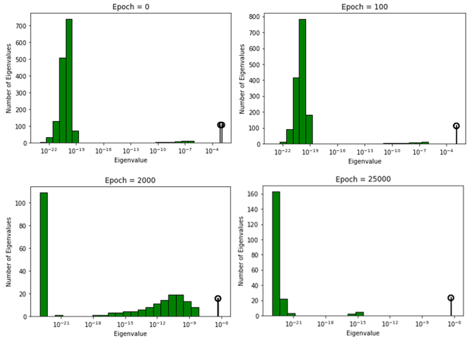
Figure 12: Histogram of the eigenvalues of the covariance of gradients $C^{(l)}$ for the Deep Linear UFM at an intermediate layer, with the top $K-1=2$ outliers plotted separately, for a range of training epochs. We see initially the top outliers are not well separated from the other eigenvalues, but over the course of training they separate and converge to the same value.

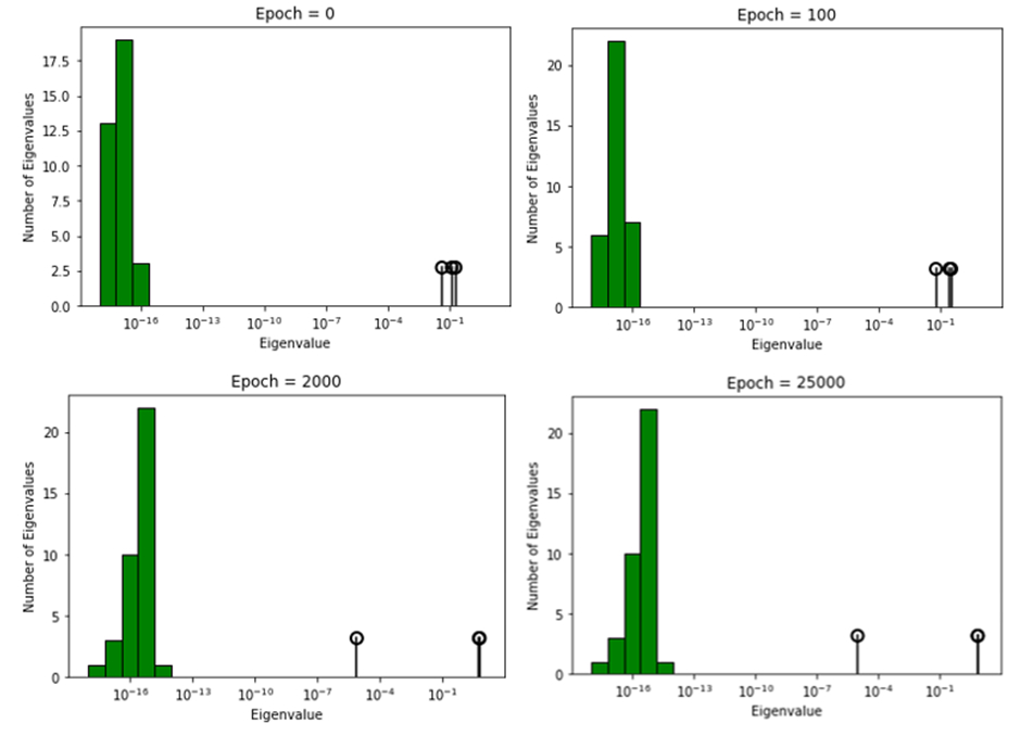
Figure 13: Histogram of the eigenvalues of the backpropagation errors matrix $\Delta^{(l)}$ for the Deep Linear UFM at an intermediate layer, with the top $K=3$ outliers plotted separately, for a range of training epochs. We see initially in training whilst the outliers are separated, they are all of similar magnitude. Over the course of training the smallest outlier separates from the others, and the remaining outliers converge to the same value.

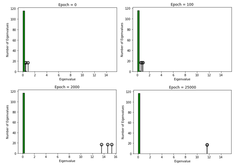
Figure 14: Histogram of the eigenvalues of the feature matrices $H^{(l)T}H^{(l)}$ for the Deep Linear UFM at an intermediate layer, with the top $K=3$ outliers plotted separately, for a range of training epochs. We see initially in training all eigenvalues are small, but as training progresses the top $K$ separate, and eventually take the same value.

G.2: Further Experiments in the Deep UFM

One of the central properties of DNC in the deep linear UFM is that the matrices $A^{(l+1)}=W_{L}...W_{l+1}\in\textbf{R}^{K\times d}$ have rows that form an orthogonal frame.

We can numerically consider whether the matrices $A^{(l+1)}$ have rows that form an orthogonal frame in the deep UFM, and compare to numerical results for the deep linear UFM. Denoting the $c^{\prime}$th row of $A^{(l+1)}$ as $a^{(l+1)}_{c^{\prime}}$ we can consider the following quantities at each layer $l$

$$r^{(l+1)}_{c^{\prime},c^{\prime\prime}}=|a^{(l+1)}_{c^{\prime}}\cdot a^{(l+1)}_{c^{\prime\prime}}|.$$

The values for the same model parameters as detailed in section 5 are given in Table 3. We see that the diagonal of the $A^{(l+1)}$ matrices is constant, which is in line with the predictions from the deep linear UFM. The off diagonal values are small by comparison, however in the deep linear UFM trained to convergence we see these be $O(10^{-5})$. Whilst it looks promising that such structure could persist in the full deep UFM, it is unclear from the numerics if this only approximately would hold.

Recall from section F.1 that in the deep UFM the $A^{(l+1)}$ matrices are in fact updated to depend on the training points, $\tilde{A}_{ic}^{(l+1)}=\tilde{W}_{L}...\tilde{W}_{l+1}$, where

$$(\tilde{W}_{l})_{xy}=(W_{l})_{xy}1((h^{l}_{ic})_{y}>0).$$

We can also ask if the rows of these matrices form an orthogonal frame for each value of the index’s $i,c$. Denote as before the $c^{\prime}$th row of $\tilde{A}_{ic}^{(l+1)}$ as $\tilde{a}_{icc^{\prime}}$. By averaging over the data, we can consider the following quantities at each layer

$$\tilde{r}^{(l+1)}_{c^{\prime},c^{\prime\prime}}=\textrm{Av}_{ic}\{|\tilde{a}^{(l+1)}_{icc^{\prime}}\cdot\tilde{a}^{(l+1)}_{icc^{\prime\prime}}|\}.$$

The values for the same parameters as before are given in Table 4. Note if each of the $\tilde{A}_{ic}^{(l+1)}$ have rows forming an orthogonal frame, then this should also be true after averaging. Instead we see from the table that these matrices do not consistently form an orthogonal frame, since the diagonal is not constant. As a consequence it seems unlikely that these matrices individually form orthogonal frames at the global optima.

Table 3: values of the quantities $r^{(l+1)}_{c^{\prime},c^{\prime\prime}}$ for the deep UFM after $10^{6}$ training epochs.

Table 4: values of the quantities $\tilde{r}^{(l+1)}_{c^{\prime},c^{\prime\prime}}$ for the deep UFM after $10^{6}$ training epochs.

References

- [1] Alex Krizhevsky, Ilya Sutskever, and Geoffrey E Hinton. Imagenet classification with deep convolutional neural networks. In Advances in Neural Information Processing Systems, volume 25. Curran Associates, Inc., 2012.
- [2] Ian Goodfellow, Yoshua Bengio, and Aaron Courville. Deep Learning. MIT Press, 2016. http://www.deeplearningbook.org.
- [3] Tom Brown, Benjamin Mann, Nick Ryder, Melanie Subbiah, Jared D Kaplan, Prafulla Dhariwal, Arvind Neelakantan, Pranav Shyam, Girish Sastry, Amanda Askell, and et al. Language models are few-shot learners. In Advances in Neural Information Processing Systems, volume 33, pages 1877–1901. Curran Associates, Inc., 2020.
- [4] Yann A LeCun, Léon Bottou, Genevieve B Orr, and Klaus-Robert Müller. Efficient backprop. In Neural networks: Tricks of the trade, pages 9–48. Springer, 2012.
- [5] Yann N Dauphin, Razvan Pascanu, Caglar Gulcehre, Kyunghyun Cho, Surya Ganguli, and Yoshua Bengio. Identifying and attacking the saddle point problem in high-dimensional non-convex optimization. In Advances in Neural Information Processing Systems, volume 27. Curran Associates, Inc., 2014.
- [6] Levent Sagun, Leon Bottou, and Yann LeCun. Eigenvalues of the hessian in deep learning: Singularity and beyond. arXiv preprint arXiv:1611.07476, 2016.
- [7] Levent Sagun, Utku Evci, V Ugur Guney, Yann Dauphin, and Leon Bottou. Empirical analysis of the hessian of over-parametrized neural networks. arXiv preprint arXiv:1706.04454, 2017.
- [8] Vardan Papyan. The full spectrum of deep net hessians at scale: Dynamics with sample size. ArXiv, abs/1811.07062, 2018.
- [9] Vardan Papyan. Measurements of three-level hierarchical structure in the outliers in the spectrum of deepnet hessians. arXiv preprint arXiv:1901.08244, 2019.
- [10] Vardan Papyan. Traces of class/cross-class structure pervade deep learning spectra. Journal of Machine Learning Research, 21(252):1–64, 2020.
- [11] Behrooz Ghorbani, Shankar Krishnan, and Ying Xiao. An investigation into neural net optimization via hessian eigenvalue density. In Proceedings of the 36th International Conference on Machine Learning, volume 97 of Proceedings of Machine Learning Research, pages 2232–2241. PMLR, 09–15 Jun 2019.
- [12] Stanislaw Jastrzebski, Maciej Szymczak, Stanislav Fort, Devansh Arpit, Jacek Tabor, Kyunghyun Cho, and Krzysztof Geras. The break-even point on optimization trajectories of deep neural networks. arXiv preprint arXiv:2002.09572, 2020.
- [13] Xinyan Li, Qilong Gu, Yingxue Zhou, Tiancong Chen, and Arindam Banerjee. Hessian based analysis of sgd for deep nets: Dynamics and generalization. In Proceedings of the 2020 SIAM International Conference on Data Mining, pages 190–198. SIAM, 2020.
- [14] Samet Oymak, Zalan Fabian, Mingchen Li, and Mahdi Soltanolkotabi. Generalization guarantees for neural networks via harnessing the low-rank structure of the jacobian. arXiv preprint arXiv:1906.05392, 2019.
- [15] Michael Mahoney and Charles Martin. Traditional and heavy tailed self regularization in neural network models. In Proceedings of the 36th International Conference on Machine Learning, volume 97 of Proceedings of Machine Learning Research, pages 4284–4293. PMLR, 09–15 Jun 2019.
- [16] Adepu Ravi Sankar, Yash Khasbage, Rahul Vigneswaran, and Vineeth N Balasubramanian. A deeper look at the hessian eigenspectrum of deep neural networks and its applications to regularization. Proceedings of the AAAI Conference on Artificial Intelligence, 35(11):9481–9488, May 2021.
- [17] Guy Gur-Ari, Daniel A. Roberts, and Ethan Dyer. Gradient descent happens in a tiny subspace. ArXiv, abs/1812.04754, 2018.
- [18] Gerard Ben Arous, Reza Gheissari, Jiaoyang Huang, and Aukosh Jagannath. High-dimensional SGD aligns with emerging outlier eigenspaces. In The Twelfth International Conference on Learning Representations, 2024.
- [19] Romain Cosson, Ali Jadbabaie, Anuran Makur, Amirhossein Reisizadeh, and Devavrat Shah. Gradient descent for low-rank functions. ArXiv, abs/2206.08257, 2022.
- [20] Tao Li, Lei Tan, Zhehao Huang, Qinghua Tao, Y. Liu, and X. Huang. Low dimensional trajectory hypothesis is true: Dnns can be trained in tiny subspaces. IEEE Transactions on Pattern Analysis and Machine Intelligence, 45:3411–3420, 2022.
- [21] Vardan Papyan, Xuemei Han, and David L. Donoho. Prevalence of neural collapse during the terminal phase of deep learning training. Proceedings of the National Academy of Sciences of the United States of America, 117:24652 – 24663, 2020.
- [22] X.Y. Han, Vardan Papyan, and David L. Donoho. Neural collapse under MSE loss: Proximity to and dynamics on the central path. In International Conference on Learning Representations, 2022.
- [23] Hangfeng He and Weijie Su. A law of data separation in deep learning. Proceedings of the National Academy of Sciences of the United States of America, 120, 2022.
- [24] Akshay Rangamani, Marius Lindegaard, Tomer Galanti, and Tomaso A Poggio. Feature learning in deep classifiers through intermediate neural collapse. In Proceedings of the 40th International Conference on Machine Learning, volume 202 of Proceedings of Machine Learning Research, pages 28729–28745. PMLR, 23–29 Jul 2023.
- [25] Liam Parker, Emre Onal, Anton Stengel, and Jake Intrater. Neural collapse in the intermediate hidden layers of classification neural networks. ArXiv, abs/2308.02760, 2023.
- [26] Vignesh Kothapalli, Ebrahim Rasromani, and Vasudev Awatramani. Neural collapse: A review on modelling principles and generalization. Trans. Mach. Learn. Res., 2023, 2022.
- [27] Dustin G. Mixon, Hans Parshall, and Jianzong Pi. Neural collapse with unconstrained features. Sampling Theory, Signal Processing, and Data Analysis, 20, 2020.
- [28] Hien Dang, Tan Minh Nguyen, Tho Tran, Hung The Tran, Hung Tran, and Nhat Ho. Neural collapse in deep linear networks: From balanced to imbalanced data. In International Conference on Machine Learning, 2023.
- [29] Peter Súkeník, Marco Mondelli, and Christoph H Lampert. Deep neural collapse is provably optimal for the deep unconstrained features model. In Advances in Neural Information Processing Systems, volume 36, pages 52991–53024. Curran Associates, Inc., 2023.
- [30] Tom Tirer and Joan Bruna. Extended unconstrained features model for exploring deep neural collapse. In International Conference on Machine Learning, 2022.
- [31] Jinxin Zhou, Xiao Li, Tianyu Ding, Chong You, Qing Qu, and Zhihui Zhu. On the optimization landscape of neural collapse under MSE loss: Global optimality with unconstrained features. In Proceedings of the 39th International Conference on Machine Learning, volume 162 of Proceedings of Machine Learning Research, pages 27179–27202. PMLR, 17–23 Jul 2022.
- [32] Wenlong Ji, Yiping Lu, Yiliang Zhang, Zhun Deng, and Weijie J Su. An unconstrained layer-peeled perspective on neural collapse. In International Conference on Learning Representations, 2022.
- [33] Zhihui Zhu, Tianyu Ding, Jinxin Zhou, Xiao Li, Chong You, Jeremias Sulam, and Qing Qu. A geometric analysis of neural collapse with unconstrained features. In Advances in Neural Information Processing Systems, volume 34, pages 29820–29834. Curran Associates, Inc., 2021.
- [34] Can Yaras, Peng Wang, Zhihui Zhu, Laura Balzano, and Qing Qu. Neural collapse with normalized features: A geometric analysis over the riemannian manifold. In Advances in Neural Information Processing Systems, volume 35, pages 11547–11560. Curran Associates, Inc., 2022.
- [35] Jinxin Zhou, Chong You, Xiao Li, Kangning Liu, Sheng Liu, Qing Qu, and Zhihui Zhu. Are all losses created equal: A neural collapse perspective. In Advances in Neural Information Processing Systems, volume 35, pages 31697–31710. Curran Associates, Inc., 2022.
- [36] Christos Thrampoulidis, Ganesh Ramachandra Kini, Vala Vakilian, and Tina Behnia. Imbalance trouble: Revisiting neural-collapse geometry. In Advances in Neural Information Processing Systems, volume 35, pages 27225–27238. Curran Associates, Inc., 2022.
- [37] Yibo Yang, Shixiang Chen, Xiangtai Li, Liang Xie, Zhouchen Lin, and Dacheng Tao. Inducing neural collapse in imbalanced learning: Do we really need a learnable classifier at the end of deep neural network? In Advances in Neural Information Processing Systems, volume 35, pages 37991–38002. Curran Associates, Inc., 2022.
- [38] Cong Fang, Hangfeng He, Qi Long, and Weijie J. Su. Exploring deep neural networks via layer-peeled model: Minority collapse in imbalanced training. Proceedings of the National Academy of Sciences of the United States of America, 118, 2021.
- [39] Léon Bottou, Frank E Curtis, and Jorge Nocedal. Optimization methods for large-scale machine learning. SIAM review, 60(2):223–311, 2018.
- [40] Jeffrey Pennington and Pratik Worah. The spectrum of the fisher information matrix of a single-hidden-layer neural network. In S. Bengio, H. Wallach, H. Larochelle, K. Grauman, N. Cesa-Bianchi, and R. Garnett, editors, Advances in Neural Information Processing Systems, volume 31. Curran Associates, Inc., 2018.
- [41] Nicholas P Baskerville, Jonathan P Keating, Francesco Mezzadri, Joseph Najnudel, and Diego Granziol. Universal characteristics of deep neural network loss surfaces from random matrix theory. Journal of Physics A: Mathematical and Theoretical, 55(49):494002, 2022.
- [42] Anna Choromanska, MIkael Henaff, Michael Mathieu, Gerard Ben Arous, and Yann LeCun. The Loss Surfaces of Multilayer Networks. In Proceedings of the Eighteenth International Conference on Artificial Intelligence and Statistics, volume 38 of Proceedings of Machine Learning Research, pages 192–204, San Diego, California, USA, 09–12 May 2015. PMLR.
- [43] Nicholas P Baskerville, Jonathan P Keating, Francesco Mezzadri, and Joseph Najnudel. The loss surfaces of neural networks with general activation functions. Journal of Statistical Mechanics: Theory and Experiment, 2021(6):064001, 2021.
- [44] Zhou Fan and Zhichao Wang. Spectra of the conjugate kernel and neural tangent kernel for linear-width neural networks. In Advances in Neural Information Processing Systems, volume 33, pages 7710–7721. Curran Associates, Inc., 2020.
- [45] Arthur Jacot, Franck Gabriel, and Clement Hongler. The asymptotic spectrum of the hessian of dnn throughout training. In International Conference on Learning Representations, 2020.
- [46] Yikai Wu, Xingyu Zhu, Chenwei Wu, Annie Wang, and Rong Ge. Dissecting hessian: Understanding common structure of hessian in neural networks. ArXiv, abs/2010.04261, 2020.