The Overlap Gap Property limits limit swapping in QAOA

Abstract

The Quantum Approximate Optimization Algorithm (QAOA) is a quantum algorithm designed for combinatorial optimization problem. We show that under the assumption that the Overlap Gap Property (OGP) in the solution space for the Max-$q$-XORSAT is a monotonic increasing function, the swapping of limits in QAOA leads to suboptimal results limited by the OGP. Furthermore, since the performance of QAOA for the pure $q$-spin model matches asymptotically for Max-$q$-XORSAT on large-girth regular hypergraph, we show that the average-case value obtained by QAOA for the pure $q$-spin model for even $q\geq 4$ is bounded away from optimality even when the algorithm runs indefinitely. This suggests that a necessary condition for the validity of limit swapping in QAOA is the absence of OGP in a given combinatorial optimization problem. A corollary of this is that the spectral gap of a Hamiltonian exhibiting the OGP will close in the thermodynamic limit resulting in a limitation of the quantum adiabatic theorem and efficient optimization of QAOA parameters. Furthermore, the results suggests that even when sub-optimised, the performance of QAOA on spin glass is equal in performance to Montanari’s classical algorithm in solving the mean field spin glass problem, the best known classical algorithm.

1 Introduction

Combinatorial Optimization Problems (COPs) are notoriously difficult even as a decision problem [1] — well known examples include the travelling salesman problem [2] and finding the ground state of a spin glass Hamiltonian [3]. Rather than attempting to find an exact solution, one is rather often interested in approximate solutions. One such algorithm is the Quantum Approximate Optimization Algorithm (QAOA) introduced by Farhi [4].

Attempting to evaluate the expectation value of QAOA is incredibly difficult. Naively, for each layer $p$ in QAOA, one would need to sum over $2^{N}$ terms. In a series of works starting with [5], algorithms to evaluate the expectation value of QAOA on $q$-spin glass models for any arbitrary parameters $(\boldsymbol{\gamma,\beta})$ with time complexity independent of $N$ have been found with increasing performance in terms of time complexity. The best known one for evaluating $q$-spin glass is found in [6] with a time complexity of $\mathcal{O}(p^{2}4^{p})$ using algebraic techniques.

Another line of research is to prove the limitation of QAOA via the Overlap Gap Property (OGP). One of the first applications to show the limitation of QAOA is when QAOA does not see the whole graph that a COP is based on [7]. The limitation of QAOA as a result of OGP has been predominately used on sparse graphs but a breakthrough came in [8] using a dense-from-sparse relation between complete graphs and sparse graphs to show that QAOA is also limited in performance even if it sees the whole graph.

In this paper, we note that the current research seems to suggest that for the $q$-spin glass model, QAOA is unlikely to find the optimal value even if $p$ goes to infinity for even $q\geq 4$ if we swap the order of limits, the thermodynamic limit and the run time of the algorithm. We will present the argument here. The paper is organised as follows: In section 2 we give a brief background to spin glasses, random graphs, Max-q-XORSAT, OGP, and QAOA; in section 3, we summarize what is known in literature about the results of QAOA on spin glasses and Max-$q$-XORSAT problems and their equivalence; in section 4 we formalize a point about OGP in random regular hypergraphs that was mentioned in [6] and show that if their observation is true, QAOA cannot find the optimal value in a dense graph even if the algorithm runs indefinitely under limit swapping. Following which, we outline a proof to affirm the theorem where the proof relies on a conjecture about the monotonicity of the OGP in Max-$q$-XORSAT while providing some numerical evidence.

1.1 Statement of result

The main result of this work is to show that the OGP exists for Max-$q$-XORSAT on a random regular hypergraph with sufficiently large degree.

Conjecture 1.1.

The OGP of Max-$q$-XORSAT on any graph is a monotonic increasing property in the sense that if the graph $G$ exhibits the overlap gap property, then adding an additional edge does not destroy the graph exhibiting the OGP i.e. $G+e$ exhibits the OGP.

We include 1.1 as the proof of our main theorem requires this to be true. It is likely to be true as it is a monotonic increasing property of Erdös–Rényi graph and in the large degree limit, the two are similar. Assuming this conjecture is true, our main theorem can be summarise as follows:

Theorem 1.2 (Informal).

When $q\geq 4$ and is even, the OGP is present for Max-$q$-XORSAT $D$-regular $q$-uniform hypergraphs and the performance of QAOA is limited at logarithmic depth.

There are several immediate corollaries of this result for QAOA. The first of which was noted in [6] as a side-note.

Corollary 1.2.1.

Optimising QAOA using the algorithm in [6, 8] only allows it to perform as well as the best classical algorithm even if the algorithm runs indefinitely.

The above corollary is a result of optimising QAOA under limit swapping of the algorithm run time and the problem size $n$. This therefore results in the following 2 corollaries:

Corollary 1.2.2.

If a COP exhibit the OGP, then optimising QAOA via limit swapping results in sub-optimal performance

Corollary 1.2.3.

The failure of QAOA under limit swapping implies that a reduction to the quantum adiabatic algorithm is not possible (i.e. the spectral gap closes).

2 Background

2.1 Spin glass

The study of mean field spin glasses is a very rich discipline in theoretical physics [9]. The main goal, roughly speaking, is to find the ground state energy of a spin glass Hamiltonian. One of the earliest example is the Edwards–Anderson model [10] which considers nearest neighbour interaction of an Ising model with the coupling strength $J_{jk}$ following a normal distribution of mean 0 and variance 1. A widely studied model is the Sherrington–Kirkpatrick (SK) model which is the infinite range version of the Edwards–Anderson model [11]

$$H_{SK}(\boldsymbol{z})=\frac{1}{\sqrt{N}}\sum_{j<k}J_{jk}z_{j}z_{k}.$$ (1)

More generally, an Ising $q$-spin model is given by the following

$$H_{q}(\boldsymbol{z})=\frac{1}{\sqrt{N^{(q-1)}}}\sum_{j<k<\dots<q}J_{jk\dots q}z_{j}z_{k}\dots z_{q},$$ (2)

with the couplings randomly chosen over a normal distribution.

To find the ground state energy, one can use the non-rigourous replica trick resulting in the replica symmetric solution using the fact that the free energy is, in principle, given by

$$-\beta F=\log Z=\lim_{N\rightarrow\infty}\lim_{n\rightarrow 0}\frac{Z^{n}-1}{nN}.$$ (3)

In practice, one instead swaps the order of the limits to use a saddle-point approximation [12, 13]

$$\lim_{n\rightarrow 0}\lim_{N\rightarrow\infty}\frac{Z^{n}-1}{nN}.$$ (4)

For the SK model, gives us an unstable solution at low temperature. An alternate solution, now known as the Parisi ansatz [14], was proven by Talagrand to give the correct solution for the even $q$ case [15] and later generalized to all $q$ by Panchenko [16]. Denote by $\mathcal{M}$ the collection of all cumulative distribution functions $\alpha$ on $[0,1]$, the Parisi formula [15] states that

$$F(\beta)=\lim_{N\rightarrow\infty}F(\beta,N)=\inf_{\alpha\in\mathcal{M}}\mathcal{P}(\beta,\alpha)\quad a.s.$$ (5)

where $\mathcal{P}$ is the so-called Parisi measure.

Thus, letting $\Sigma_{N}=\{-1,+1\}^{N}$, the ground state energy can be found via the following equation

$$\lim_{N\rightarrow\infty}\max_{\boldsymbol{z}\in\Sigma_{N}}\frac{H(\boldsymbol{z})}{N}=\lim_{\beta\rightarrow\infty}F(\beta)=\lim_{\beta\rightarrow\infty}\inf_{\alpha\in\mathcal{M}}\mathcal{P}(\beta,\alpha).$$ (6)

For the $q$-spin model, the limit can be computed explicitly which we denote as the Parisi constant

$$\Pi_{q}=\lim_{N\rightarrow\infty}\max_{\boldsymbol{z}\in\Sigma_{N}}\frac{H_{q}(\boldsymbol{z})}{N}.$$ (7)

2.2 Random Graphs

Here we standardize the notation we use to denote a hypergraph. Conventionally, an instance of the Erdös–Rényi–(Gilbert) $q$-uniform hypergraph $\mathbb{G}^{q}_{ER}(n,p)$ is a random graph with $n$ vertices where each hyperedge is added with probability $p$. The original Erdös–Rényi $q$-uniform hypergraph $\mathbb{G}^{q}_{ER}(n,m)$ is chosen randomly from the set of hypergraph with $n$ vertices and $m$ hyperedges. The former is now more frequently used. The two types of Erdös–Rényi graphs are similar to each other when $np=m$. In fact, it has been shown that the two types of random graphs are asymptotically equivalent under certain conditions [17]. We will use the former definition unless otherwise mentioned.

Another type of random hypergraph of interest is the $d$-regular $q$-uniform hypergraph $\mathbb{R}^{q}(n,d)$ where we implicitly assume that $nd=qm$ for some integer $m$. Unlike Erdös–Rényi graphs that can be generated randomly, there is no easy unbiased way to generate such graphs, though one such method is known as the configuration model introduced by Bollobás [18].

2.3 MaxCUT and Max-q-XORSAT

Given a graph $G=(V,E)$, the MaxCUT problem is to partition the vertices $V$ into $V=V_{1}\cup V_{2}$ such that the number of edges between $V_{1}$ and $V_{2}$ is maximised. The cost function for MaxCUT is

$$H_{MC}(\boldsymbol{z})=\sum_{(u,v)\in E}\frac{1}{2}(1-z_{u}z_{v}).$$ (8)

For random instances of MaxCUT, one usually chooses either from Erdös–Rényi or random regular graph ensembles. In the large degree limit, for both $\mathbb{G}^{q}_{ER}(n,p)$ and $\mathbb{R}^{q}(n,d)$, it has been shown that with high probability, as $n\rightarrow\infty$ [19],

$$\frac{\text{MaxCUT}(G)}{|E|}=\frac{1}{2}+\Pi_{2}\sqrt{\frac{1}{d}}+\mathcal{O}(1/\sqrt{d}),$$ (9)

where $\Pi_{2}=0.7631\dots$ is the Parisi value for the SK model.

Generalising MaxCUT, we have the XOR-satisfiability (XORSAT) problem. Specifically, given a $q$-uniform hypergraph $G=(V,E)$ where $E\subset V^{q}$, and a given signed weight $J_{i_{1},\dots,i_{q}}\in\{-1,+1\}$, Max-$q$-XORSAT is the problem of maximising the following cost function

$$H_{XOR}^{q}(\boldsymbol{z})=\sum_{(i_{1},\dots,i_{q})\in E}\frac{1}{2}(1+J_{i_{1}i_{2}\dots i_{q}}z_{i_{1}}z_{i_{2}}\dots z_{i_{q}}).$$ (10)

The cost function is essentially counting the number of satisfied clauses where a clause is satisfied if $z_{i_{1}}z_{i_{2}}\dots z_{i_{q}}=J_{i_{1}i_{2},\dots i_{q}}$ for a given hyperedge. MaxCUT is thus a special case of this problem with $q=2$ and $J_{i_{1}i_{2}}=-1$.

We say that an instance of the problem is satisfied if there is an assignment of values to the bit-string $\boldsymbol{z}$ which satisfies all the clauses (i.e. $H_{XOR}^{q}(\boldsymbol{z})=|E|$), otherwise, we say it is unsatisfiable. It is known that for an instance $\xi$ of a random $q$-XORSAT problem, given $|E|$ hyperedges and problem size $n$, the following theorem holds

Theorem 2.1 (Theorem 1 of [20]).

Let $q>2$ be fixed. Let $|E|/n=\delta$. In the limit $n\rightarrow\infty$,

1. if $\delta>1$, then a random formula from $\xi$ is unsatisfiable with high probability

2. if $\delta<1$, then a random formula from $\xi$ is satisfiable with high probability.

For a random $d$-regular $q$-uniform hypergraph, this condition implies that if $d>q$, then a random formula is unsatisfiable with high probability. Suppose we fix $d>q$ sufficiently large so that we are in the unsatisfiability regime. The maximum number of satisfiable equations in an instance of random XORSAT has been found [21] to be

$$\frac{1}{|E|}\max_{\boldsymbol{z}}H_{XOR}^{q}(\boldsymbol{z})=\frac{1}{2}+\Pi_{q}\sqrt{\frac{q}{2d}}+\mathcal{O}(1/\sqrt{d})$$ (11)

2.4 Overlap Gap Property

One major obstacle to finding optimal solutions for COPs is known as the Overlap Gap Property (OGP). The term was introduced in [22], though the concept was already used by various authors [23, 24].

To understand OGP, consider the overlap of two big-string configurations (or spin configurations):

$$|R_{1,2}|=\left|\frac{1}{N}\sum_{i=1}^{N}\boldsymbol{z}_{i}^{1}\boldsymbol{z}_{i}^{2}\right|=\left|\frac{\boldsymbol{z}^{1}\cdot\boldsymbol{z}^{2}}{N}\right|.$$ (12)

We see that

$$R_{1,2}\approx\begin{cases}0&\quad\boldsymbol{z}^{1},\boldsymbol{z}^{2}\text{ almost totally uncorrelated},\\ 1&\quad\boldsymbol{z}^{1},\boldsymbol{z}^{2}\text{ almost totally (anti-)correlated}.\end{cases}$$ (13)

The overlap is thus a measure of how much correlation there is between two different configurations are.

For the definition of the OGP, one can informally think that for certain choices of disorder $J$, there is a gap in the set of possible pairwise overlaps of near-optimal solution. For every two $\epsilon$ optimal solution $\boldsymbol{z}^{1},\boldsymbol{z}^{2}$, it is the case that the distance between them is either extremely small, or extremely large. Formally, we define OGP for a single instance as the following:

Definition 2.1 (Overlap Gap Property [25]).

For a general maximization problem with random input $J$

$$\max_{\boldsymbol{z}\in 2^{n}}H_{J}(\boldsymbol{z}),$$ (14)

the OGP holds if there exists some $\epsilon>0,$ with $0\leq\mu_{1}<\mu_{2}$ such that for every $\boldsymbol{z}^{1},\boldsymbol{z}^{2}$ that is an $\epsilon$-optimal solution

$$H_{J}(\boldsymbol{z}^{i})\geq\max_{\boldsymbol{z}\in 2^{n}}H_{J}(\boldsymbol{z})-\epsilon,$$ (15)

it holds that the overlap between them is either less than $\mu_{1}$ or greater than $\mu_{2}$

$$R_{1,2}\in[0,\mu_{1}]\cup[\mu_{2},1).$$ (16)

The first interval is trivial as we can simply choose the overlap $\boldsymbol{z}^{1}$ with itself. It is the existence of the second overlap, or rather the non-existence of overlap in the interval $(\mu_{1},\mu_{2})$, that is difficult to prove.

A more general version of it is known as the ensemble-OGP introduced in [26] or coupled-OGP as used in [27]. This version is required to prove limitations of local algorithm for technical reasons and requires an interpolation scheme as defined below for interpolating between two different instances of Erdös–Réyni graphs.

Definition 2.2 (Coupled Interpolation[26]).

A coupled interpolation between a pair of hypergraphs $(G_{1},G_{2})$ with connectivity $\lambda$ is generated as follows

1. First, generate a number sampled from $x=\text{Poisson}(t\lambda n)$ with $t\in[0,1]$, and choose $x$ random $q$-hyperedges uniformly drawn from the set $[n]^{q}$ and put in a set $E$.

2. Next, generate two more random numbers $y,z$ from $\text{Poisson}((1-t)\lambda n)$, and those numbers of random q-hyperedges are independently drawn from $[n]^{q}$ to form the sets $E_{1}$ and $E_{2}$ respectively.

3. Lastly, the coupled hypergraphs are constructed as $G_{1}=(V,E\cup E_{1})$ and $G_{2}=(V,E\cup E_{2})$.

Definition 2.3 (coupled-OGP [25]).

For a set of problem instances $\chi$ related via the coupled interpolation, we say that it satisfies the e-OGP criteria if for every pair of instances $\phi,\psi\in\chi$, there exists some $\epsilon>0,$ with $0\leq\mu_{1}<\mu_{2}$ such that for every $\epsilon$-optimal solution $\boldsymbol{z}^{1}$ for instance $\phi$ and $\epsilon$-optimal solution $\boldsymbol{z}^{2}$ of instance $\psi$, it holds that the overlap between them is either less than $\mu_{1}$ or greater than $\mu_{2}$

$$R_{1,2}\in[0,\mu_{1}]\cup[\mu_{2},1).$$ (17)

where the former case is not possible if they are probabilistic independent (i.e. $t=0$).

Remark.

The standard OGP is a special case when $t=1$ so that both graphs are identical and we really only have a single instance.

2.5 QAOA

The QAOA is a quantum algorithm introduced in [4] to find approximate solutions to combinatorial optimization problems. The goal is to find a bit string $\boldsymbol{z}\in\{-1,+1\}^{N}$ that maximizes the cost function $C(\boldsymbol{z})$. Given a classical cost function $C$, we can define a corresponding quantum operator $C$ that is diagonal in the computational basis, $C\ket{\boldsymbol{z}}=C(\boldsymbol{z})\ket{\boldsymbol{z}}$. In addition, define the operator $B=\sum_{j}^{N}X_{j}$ where $X_{j}$ is the Pauli $X$ operator acting on qubit $j$. Given a set of parameters $\boldsymbol{\gamma}=(\gamma_{1},\dots,\gamma_{p})\in\mathbb{R}^{p}$ and $\boldsymbol{\beta}=(\beta_{1},\dots,\beta_{p})\in\mathbb{R}^{p}$, the QAOA prepares the initial state as $\ket{s}=\ket{+}^{N}=2^{-N/2}\sum_{\boldsymbol{z}}\ket{\boldsymbol{z}}$ and applies $p$ layers of alternating unitary operators $e^{-i\gamma_{k}C}$ and $e^{-i\beta_{k}B}$ to prepare the state

$$\ket{\boldsymbol{\gamma,\beta}}=e^{-i\beta_{p}B}e^{-i\gamma_{p}C}\dots e^{-i\beta_{1}B}e^{-i\gamma_{1}C}\ket{s}.$$ (18)

For a given cost function $C$, the corresponding QAOA objective function is the expectation value $\expectationvalue{C}{\boldsymbol{\gamma,\beta}}$. Preparing the state $\ket{\boldsymbol{\gamma,\beta}}$ and measuring in the computational basis will yield a bit string $\boldsymbol{z}$ near the quantum expectation value. Heuristics strategies to optimize $\expectationvalue{C}{\boldsymbol{\gamma,\beta}}$ with respect to $(\boldsymbol{\gamma,\beta})$ using a good initial guess have been proposed in [28].

3 Summary of known theorems

3.1 QAOA and spin glass

In [5], by applying QAOA on the Sherrington–Kirkpatrick (SK) model, the authors found an algorithm to evaluate the expectation value in the infinite limit after averaging over the disorder $\mathbb{E}_{J}$. Namely

Theorem 3.1 ([5]).

For any $p$ and any parameters $(\boldsymbol{\gamma,\beta})$, we have

$$\lim_{n\rightarrow\infty}\mathbb{E}_{J}\left[\expectationvalue{H_{SK}/N}{\boldsymbol{\gamma,\beta}}\right]=V_{p}(\boldsymbol{\gamma,\beta}),$$ (19)

where $H_{SK}$ is the the classical cost function of the SK model as defined earlier.

Furthermore, they also showed that

$$\lim_{n\rightarrow\infty}\mathbb{E}_{J}\left[\expectationvalue{(H_{SK}/N)^{2}}{\boldsymbol{\gamma,\beta}}\right]=\left[V_{p}(\boldsymbol{\gamma,\beta})\right]^{2}.$$ (20)

As a Corollary, this implies that QAOA concentrates over measurements and instances as $N\rightarrow\infty$.

More generally, for a $q$-spin glass with cost function

$$H_{q}(\boldsymbol{z})=\frac{1}{\sqrt{N^{(q-1)}}}\sum_{j<k<\dots<q}J_{jk\dots q}z_{j}z_{k}\dots z_{q},$$ (21)

it was shown in [8] that the following theorem holds

Theorem 3.2.

[Theorem 1 of [8]] For any $p$ and any parameters $(\boldsymbol{\gamma,\beta})$, we have

$$\lim_{n\rightarrow\infty}\mathbb{E}_{J}\left[\expectationvalue{H_{q}/N}{\boldsymbol{\gamma,\beta}}\right]=V^{(q)}_{p}(\boldsymbol{\gamma,\beta}),$$ (22)

Furthermore, they also showed that

$$\lim_{n\rightarrow\infty}\mathbb{E}_{J}\left[\expectationvalue{(H_{q}/N)^{2}}{\boldsymbol{\gamma,\beta}}\right]=\left[V^{(q)}_{p}(\boldsymbol{\gamma,\beta})\right]^{2}.$$ (23)

3.2 QAOA and Max-q-XORSAT

In [6], the authors evaluated the performance of QAOA for MaxCut on large-girth $(D+1)$-regular graphs. By restricting to graphs that are regular and girth (also known as the shortest Berge-cycle) greater than $2p+1$, the subgraph explored by QAOA at depth $p$ will appear as regular trees.

For large $D$, such that we are in the unsatisfiability limit, in order for the optimal $\gamma$ to be of order 1, it is convenient to prepare $\ket{\boldsymbol{\gamma,\beta}}$ using a scaled cost function operator

$$C=-\frac{1}{\sqrt{D}}\sum_{(u,v)\in E}Z_{u}Z_{v}.$$ (24)

Because the subgraph explored by QAOA at depth $p$ appear as trees, the cut fraction output by QAOA can thus be expressed as

$$\frac{\expectationvalue{H_{MC}}{\boldsymbol{\gamma},\boldsymbol{\beta}}}{|E|}=\frac{1}{2}-\frac{1}{2}\expectationvalue{Z_{u}Z_{v}}{\boldsymbol{\gamma},\boldsymbol{\beta}}.$$ (25)

Since the optimal cut fraction is of the form $1/2+\mathcal{O}(1/\sqrt{D})$ in a typical random graph as in eq. 11, we write

$$\frac{1}{2}\expectationvalue{Z_{u}Z_{v}}{\boldsymbol{\gamma},\boldsymbol{\beta}}=-\frac{\nu_{p}(D,\boldsymbol{\gamma},\boldsymbol{\beta})}{\sqrt{D}}.$$ (26)

Let

$$\nu_{p}(\boldsymbol{\gamma,\beta})=\lim_{D\rightarrow\infty}\nu_{p}(D,\boldsymbol{\gamma},\boldsymbol{\beta}),$$ (27)

then, we have the following theorem

Theorem 3.3 ([6]).

There exists an algorithm that uses $\mathcal{O}(p^{2}4^{p})$ time and $\mathcal{O}(p^{2})$ space to evaluate $\nu_{p}(\boldsymbol{\gamma,\beta})$ for all $(\boldsymbol{\gamma,\beta})$.

More generally, one can evaluate QAOA’s performance for Max-$q$-XORSAT on $q$-uniform, $(D+1)$-regular hypergraphs where MaxCUT is a special case.

Similar to MaxCut, one uses a scaled cost function to prepare the QAOA state

$$C=\frac{1}{\sqrt{D}}\sum_{(i_{1},\dots,i_{q})\in E}J_{i_{1}i_{2}\dots i_{q}}Z_{i_{1}}Z_{i_{2}}\dots Z_{i_{q}}$$ (28)

and with this, we state the following theorem

Theorem 3.4 (Theorem 2 of [6]).

For $H_{XOR}^{q}$ on any $(D+1)$-regular $q$-uniform hypergraphs with girth $>2p+1$, for the state $\ket{\boldsymbol{\gamma,\beta}}$ generated using the scaled cost function in eq. 28, then for any choice of $J$,

$$\frac{1}{|E|}\expectationvalue{H_{XOR}^{q}}{\boldsymbol{\gamma},\boldsymbol{\beta}}=\frac{1}{2}+\nu_{p}^{[q]}(D,\boldsymbol{\gamma},\boldsymbol{\beta})\sqrt{\frac{q}{2D}}.$$ (29)

where $\nu_{p}(D,\boldsymbol{\gamma},\boldsymbol{\beta})$ is independent of $J$. In addition, the limit

$$\nu_{p}^{[q]}(\boldsymbol{\gamma},\boldsymbol{\beta})=\lim_{D\rightarrow\infty}\nu_{p}^{[q]}(D,\boldsymbol{\gamma},\boldsymbol{\beta})$$ (30)

can be evaluated with an iteration using $\mathcal{O}(p^{2}4^{p})$ time and $\mathcal{O}(p^{2})$ space.

One point to note is that in [7], it has been shown that at low depth $p$, if a problem exhibits OGP, then the locality of QAOA makes it such that it is prevented from getting close to the optimal value if it does not see the whole graph. Specifically, the following theorem is proven

Theorem 3.5 (modified version of Corollary 4.4 in [27]).

For Max-$q$-XORSAT on a random Erdös–Réyni directed multi-hypergraph, for every even $q\geq 4$, there exists a value $\eta_{OGP}<\eta_{OPT}$, where $\eta_{OPT}$ is the energy of the optimal solution, and a sequence $\{\delta(d)\}_{d\geq 1}$ with the following property. For every $\epsilon>0$ there exists sufficiently large $d_{0}$ such that for every $d>d_{0}$, every $p\leq\delta(d)\log N$ and an arbitrary choice of parameters $\boldsymbol{\gamma,\beta}$ with probability converging to 1 as $N\rightarrow\infty$, the performance of QAOA with depth $p$ satisfies $\expectationvalue{C_{XOR}^{q}/N}{\boldsymbol{\gamma,\beta}}\leq\eta_{OGP}+\epsilon$.

The authors of [6] noted that assuming OGP also holds for regular hypergraphs, then a similar argument can be used to show that QAOA’s performance as measured by the algorithm in theorem 3.4 does not converge to the Parisi value $\Pi_{q}$ for even $q\geq 4$. This is because the large girth assumption implies that the graph has at least $D^{p}$ vertices so $p$ is always less than $\epsilon\log n$ in this limit. For instance, in $q=2$, the subgraph explored at constant $p$ has $2(D^{p}+\dots+D+1)$ vertices. This lays the foundation of theorem 4.1 later.

3.3 Equivalence of performance

Before going to the general theorem, we note that in [6], the first equivalence between spin glass and MaxCut was shown. Specifically, the following theorem was proven:

Theorem 3.6 (Theorem 1 of [6]).

For all $p$ and all parameters $(\boldsymbol{\gamma,\beta})$:

$$V_{p}(\boldsymbol{\gamma,\beta})=\nu_{p}(\boldsymbol{\gamma,\beta})$$ (31)

In other words, the performance of QAOA at depth $p$ on the SK model as $N\rightarrow\infty$ is equal to the performance of QAOA at depth $p$ on MaxCut problems on large-girth $D$-regular graphs when $D\rightarrow\infty$.

In their follow up work in [8], they generalize this result to show that QAOA’s performance for the $q$-spin model is equivalent to that for Max-$q$-XORSAT on any large girth $D$-regular hypergraphs in the limit $D\rightarrow\infty$.

Theorem 3.7 (Theorem 3 of [8]).

Let $\nu_{p}^{[q]}(\boldsymbol{\gamma},\boldsymbol{\beta})$ be the performance of QAOA on any instance of Max-$q$-XORSAT on any $d$-regular $q$-uniform hypergraphs with girth $>2p+1$ as given in [6]. Then for any $p$ and any parameters $(\boldsymbol{\gamma,\beta})$, we have

$$V^{(q)}_{p}(\boldsymbol{\gamma,\beta})=\sqrt{2}\nu_{p}^{[q]}(\sqrt{q}\boldsymbol{\gamma},\boldsymbol{\beta})$$ (32)

Remark.

The additional factor of $\sqrt{q}$ and $\sqrt{2}$ is due to the different notation of the two papers and was acknowledge in [8] that $\nu_{p}^{[q]}(\boldsymbol{\gamma},\boldsymbol{\beta})$ produced by the algorithm of theorem 3.4 matches (up to a rescaling) the formula $V^{(q)}_{p}(\boldsymbol{\gamma,\beta})$ for the pure $q$-spin model.

4 Main Results

We now have the pieces in place to state our main theorem

Theorem 4.1.

Informally, OGP is present for Max-$q$-XORSAT $D$-regular $q$-uniform hypergraphs and this means that the performance of QAOA on such problems using the iteration in theorem 3.4 does not converge to the optimal value as $p\rightarrow\infty$ for even $q\geq 4$.

Formally, for Max-$q$-XORSAT on a D-regular $q$-uniform hypergraph, for every even $q\geq 4$, there exists a value $\eta_{OGP}$ such that it is smaller than the optimal value $\eta_{OPT}$ and a sequence $\{\delta(d)\}_{d\geq 1}$ with the following property. For every $\epsilon>0$ there exists sufficiently large $d_{0}$ such that for every $d>d_{0}$, every $p\leq\delta(d)\log N$ and an arbitrary choice of parameters $\boldsymbol{\gamma,\beta}$ with probability converging to 1 as $N\rightarrow\infty$, the performance of QAOA with depth $p$ satisfies $\expectationvalue{C_{XOR}^{q}/N}{\boldsymbol{\gamma,\beta}}\leq\eta_{OGP}+\epsilon$ even if $p\rightarrow\infty$.

As a result of this theorem, then we have the following corollary:

Corollary 4.1.1.

From theorem 4.1 the performance of QAOA on the pure $q$-spin glass for even $q\geq 4$ converges to $\eta_{OGP}$ as $p\rightarrow\infty$ and is strictly less than the optimal value, i.e. the Parisi value $\Pi_{q}$, under the swapping of limits.

Proof.

From theorem 3.7, we have that the performance of QAOA at constant $p$ for $q$-spin glass is equal to any instance of Max-$q$-XORSAT on any $d$-regular $q$-uniform hypergraphs with girth $>2p+1$. This holds for any $q$. Thus, taking the limit $p\rightarrow\infty$ gives

$$\lim_{p\rightarrow\infty}V^{(q)}_{p}(\boldsymbol{\gamma,\beta})=\lim_{p\rightarrow\infty}\sqrt{2}\nu_{p}^{[q]}(\sqrt{q}\boldsymbol{\gamma},\boldsymbol{\beta})$$ (33)

By theorem 4.1, the right hand side of eq. 33 will achieve a value $\eta_{OGP}$ that is strictly less than $\Pi_{q}$ for even $q\geq 4$ so

$$\lim_{p\rightarrow\infty}\sqrt{2}\nu_{p}^{[q]}(\sqrt{q}\boldsymbol{\gamma},\boldsymbol{\beta})=\eta_{OGP}<\Pi_{q}$$ (34)

This implies that QAOA on the $q$-spin glass for even $q\geq 4$ will be strictly less than $\Pi_{q}$ and this completes the proof. ∎

We note that corollary 4.1.1 shows that QAOA will not be able to find the optimal value even when it sees the whole graph and the algorithm runs indefinitely if one optimises the parameters of QAOA via limit swapping.

Formally, the Parisi value is attainable via QAOA with the following limits:

$$\lim_{N\rightarrow\infty}\lim_{p\rightarrow\infty}V^{(q)}_{p}(N,\boldsymbol{\gamma,\beta})=\Pi_{q}.$$ (35)

The iteration provided in theorem 3.4 swaps the limits which results in failure of QAOA to find the optimal value. This leads us to the following corollaries

Corollary 4.1.2.

If OGP exists in a problem, then the swapping of limits results in a sub-optimal solution. In other words, a necessary condition for the validity of limit swapping is that the problem does not exhibit OGP.

Remark.

For $q$-spin glass, it is expected that OGP holds for all $q\geq 3$ which suggests that limit swapping is not allowed for all mean-field spin glasses with the possible exception for the $2$-spin glass model (i.e. the SK model).

Corollary 4.1.3.

If OGP exists for a problem, the spectral gap closes in the thermodynamic limit.

4.1 Proof of theorem

Here we set out to prove theorem 4.1. In order to do so, we need the following conjecture

Conjecture 4.2.

The OGP of Max-$q$-XORSAT on any graph is a monotonic increasing property in the sense that if the graph $G$ exhibits the overlap gap property, then adding an additional edge does not destroy the graph exhibiting the OGP i.e. $G+e$ exhibits the OGP.

Here, we outline a “proof” of the conjecture and note why this proof fails.

The theorem of the presence of the OGP for Max-$q$-XORSAT on Erdös–Rényi hypergraph is expressed as follows

Theorem 4.3 (Coupled-OGP in dilute spin glass, Theorem 5 of [26]).

Given a coupled $q$-uniform as defined in definition 2.2. For any even $q\geq 4$, there exists $0<a<b<1,\Pi_{q}>\eta_{0}>0,\lambda_{0}>0$ and $N_{0}\geq 1$ such that for any $t\in[0,1],\lambda\geq\lambda_{0},N>N_{0}$, the following holds with probability at least $1-e^{-N/L}$ for some $L=L(\eta_{0})$, that whenever two spin configurations $\boldsymbol{z}^{1},\boldsymbol{z}^{2}$ satisfy

$$\frac{H^{q}_{XOR}}{N}\geq\sqrt{\lambda}(\Pi_{q}-\eta_{0})$$ (36)

then their overlap satisfies $|R_{1,2}|\not\in[a,b]$.

From theorem 4.3, this implies that given a hypergraph $\mathbb{G}^{q}_{ER}(N,p)$, there exists $p^{*}$ such that OGP occurs with high probability as $N\rightarrow\infty$ if $p>p^{*}$. From this, we see that any additional edges preserves the presence of OGP so similarly, in $\mathbb{G}^{q}_{ER}(N,m)$, there exists an $m^{*}$ such that if $m>m^{*}$, the OGP occurs with high probability.

This seems to prove that the OGP is indeed a monotonic increasing property of a hypergraph. However, in this instance, all it says is that the appearance of the OGP is a monotonic increasing property of Erdös–Rényi hypergraphs. To immediately claim that it is also monotonically increasing for random regular hypergraphs is not entirely obvious as the edges for regular hypergraphs are not added independently of each other. However, it should be the case since for graphs with extremely high connectivity like the complete graph, it will exhibit the OGP and we can find an embedding for a random regular sub-hypergraph with smaller degree. Furthermore, as we will see later, small connectivity Erdös–Rényi hypergraphs can be embedded in random regular hypergraphs. Thus, one has two instances of $\mathbb{G}^{q}_{ER}(N,p_{1}),\mathbb{G}^{q}_{ER}(N,p_{2})$ with $p_{1}<p_{2}$ that has the OGP and also that $\mathbb{G}^{q}_{ER}(N,p_{1})\subset\mathbb{R}^{q}(N,d)\subset\mathbb{G}^{q}_{ER}(N,p_{2})$. If the OGP were not a monotonic property for random regular graphs, then at some point, we should find that the OGP fails when adding edges in an interpolation between $\mathbb{G}^{q}_{ER}(N,p_{1})$ and $\mathbb{G}^{q}_{ER}(N,p_{2})$ but that would contradict theorem 4.3. Formalising this would verify the conjecture and complete the proof. Furthermore, [29] notes that in the planted clique problem, the occurrence of OGP is related to the monotonicity of another graph property.

Another result that we need comes from the fact that we can embed an Erdös–Rényi hypergraph into a random regular hypergraph.

Theorem 4.4 (Theorem 1 and Corollary 2 of [30]).

For each $q\geq 2$ there is a positive constant $C$ such that if for some real $\gamma=\gamma(n)$ and positive integer $d=d(n)$,

$$C\left(\left(d/n^{q-1}+\log(n)/d\right)^{1/3}+1/n\right)\leq\gamma<1,$$ (37)

and $m=(1-\gamma)nd/q$ is an integer, then there is a joint distribution of $\mathbb{G}^{q}_{ER}(n,m)$ and $\mathbb{G}^{q}(n,d)$ with

$$\lim_{n\rightarrow\infty}\mathbb{P}(\mathbb{G}^{q}_{ER}(n,m)\subset\mathbb{R}^{q}(n,d))=1.$$ (38)

Furthermore, let $\mathcal{P}$ be a monotone increasing property. if $\log{n}\ll d\ll n^{q-1}$, for some $m\leq(1-\gamma)nd/q$ where $\gamma$ satisfies eq. 37, then if $\mathbb{G}^{q}_{ER}(n,m)\in\mathcal{P}$ as $n\rightarrow\infty$, then $\mathbb{R}^{q}(n,d))\in\mathcal{P}$ as $n\rightarrow\infty$.

We have to prove that our condition for large potentially infinite girth fit this condition for the embedding.

The girth $g$ of a $d$-regular $q$-uniform hypergraph is known [31] to be bounded by

$$\frac{\log{n}-\log 4}{\log(q-1)+\log(d-1)}-1<g\leq\frac{2\log n}{\log(q-1)+\log(d-1)}+2.$$ (39)

For constant $q$, an infinite girth requires $d\ll n$

Let $d\sim\mathcal{O}(n^{\epsilon})$ for sufficiently small $\epsilon>0$ and $n^{\epsilon}>q$. Such a constraint satisfies the large girth requirement. Substituting $d$ into eq. 37 gives us

$$C\left(\left(\frac{n^{\epsilon}}{n^{q-1}}+\frac{\log{n}}{n^{\epsilon}}\right)^{1/3}+1/n\right)\leq\gamma<1,$$ (40)

where in the large $n$ limit, we see that the lhs. approaches 0. Thus, for $m=(1-\gamma)nd/q\sim\mathcal{O}(n^{1+\epsilon})$, an embedding can be performed.

From this, it follows that for some $m^{*}\leq(1-\gamma)nd/q$, if $\mathbb{G}^{q}_{ER}(n,m)$ has a monotone increasing property $\mathcal{P}$, then $\mathbb{R}^{q}(n,d)$ also has it as well. For $m$ to be drawn from a Poisson distribution where the graph has connectivity $\lambda$, we require $m=n(\log n+(\lambda-1)\log\log n+c)/d\sim\mathcal{O}(n^{1-\epsilon}\log n)$ for some finite constant $c$ [32]. Thus, there exists a $d_{0}$ such that, for $d>d_{0}$, the existence of OGP is present in the solution space of Max-$q$-XORSAT on Random Regular hypergraph $\mathbb{R}^{q}(n,d)$ with high probability meaning that the result of [27] also applies to random regular hypergraphs.

4.2 Numerical evidence

Here, we provide some numerical evidence that instances of OGP can occur in random regular hypergraph. The code can be found here [33]. Our numerical simulation proceeds in the following manner. First, we define the problem size $n$, uniformity $q$, and degree $d$, where we implicitly assume that $nd$ is a multiple of $q$. Then, randomly generate a $d$-regular $q$-uniform hypergraph so that the total number of hyperdeges $|E|=(nd/q)$. Next, we randomly generate the list $\boldsymbol{J}=\{-1,+1\}^{|E|}$ for the coupling strength of the hyperedges. Finally, we perform a branch and bound algorithm and record those whose cut-fraction exceeds a certain threshold. Since the maximum fraction of satisfied clauses is asymptotically equal to eq. 11, we define a cut-off point that a bit-string should return a cut-fraction > 0.8.

Once we have the list of bit-strings and their corresponding cut-fraction, we have to choose some $\epsilon>0$ such that the list of bit-strings that are $\epsilon$-optimal solutions is small. By default, we limit the bit-strings that are at least 95% to the optimal solution. Finally, compute the overlap between all such $\epsilon$-optimal bit-string and obtain the overlap spectrum.

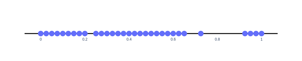
(a) $n=40$ with constant degree $10$ .

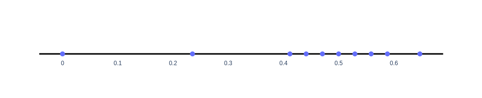
(b) $n=34$ with constant degree $10$ .

Figure 1: Typical spectrum of Overlap obtained in $4$-uniform random regular graphs. Subgraph a included the next 2 optimal solution while subgraph b included only the first suboptimal solutions to show how the overlap spectrum typically evolves as we included more suboptimal solutions.

We find that on average, when $d<q$, OGP is not present. It is only when $d$ is greater than $q$ that instances of problems exhibiting OGP first appears. The numerical simulations was run on $q=4$ and varying $n$ up till 40.

We also ran simulations on the SK model as is it highly believed, though not yet proven, that the SK model does not exhibit the OGP [3, 34]. Modulo the $\mathbb{Z}_{2}$ symmetry, we find that indeed the SK model does not exhibit the OGP at $n=45$.

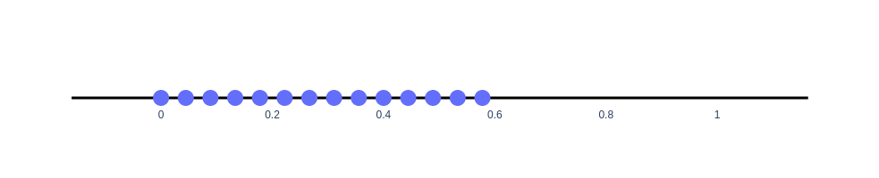
Figure 2: The overlap spectrum of an instance of the SK model with $=45$.

5 Discussion and further work

Being a heuristic algorithm, the limitations and potential of QAOA have not yet been fully explored. While swapping the order of limits allows us to evaluate the expectation value with a classical computer faster, it also seems to lead to sub-optimal results. This of course is expected and one can instead use the algorithm developed in [6] as a heuristic starting ansatz for $(\boldsymbol{\gamma,\beta})$ to be further optimized for a specific problem.

Our proof relies on a conjecture that is likely to be true based on numerical results and similarities with other graphs in the large degree limit. Proving that the OGP for the Max-$q$-XORSAT is also a monotonic increasing property on random $d$-regular $q$-uniform hypergraphs would formalized this proof and show definitively that the presence of OGP prevents the swapping of limits.

This result come from a “dense-from-sparse” reduction first performed in [8]. It remains an open problem to show that OGP is a limitation on dense model without the need to rely on this reduction.

We note that under limit swapping, the performance of QAOA equals that of Montanari’s AMP algorithm for the mean field spin glass [34]. This suggests that if QAOA is optimized correctly, it should outperform the best classical algorithm. It is still an open question to determine at what depth $p$ will QAOA outperform the AMP algorithm. Furthermore, given the similarity in performance to the AMP algorithm, this also suggests that the conjecture in [6] that the Parisi value for the Sherrington–Kirkpatrick model is obtained under limit swapping might be true.

References

- [1] R. M. Karp, Reducibility among Combinatorial Problems. Boston, MA: Springer US, 1972, pp. 85–103. [Online]. Available: https://doi.org/10.1007/978-1-4684-2001-2_9
- [2] J. Steele, Probability Theory and Combinatorial Optimization, ser. CBMS-NSF Regional Conference Series in Applied Mathematics. Society for Industrial and Applied Mathematics, 1997. [Online]. Available: https://books.google.de/books?id=inyEeSEqqtwC
- [3] D. Gamarnik, C. Moore, and L. Zdeborová , “Disordered systems insights on computational hardness,” Journal of Statistical Mechanics: Theory and Experiment, vol. 2022, no. 11, p. 114015, nov 2022. [Online]. Available: https://doi.org/10.1088%2F1742-5468%2Fac9cc8
- [4] E. Farhi, J. Goldstone, and S. Gutmann, “A quantum approximate optimization algorithm,” 2014.
- [5] E. Farhi, J. Goldstone, S. Gutmann, and L. Zhou, “The Quantum Approximate Optimization Algorithm and the Sherrington-Kirkpatrick Model at Infinite Size,” Quantum, vol. 6, p. 759, Jul. 2022. [Online]. Available: https://doi.org/10.22331/q-2022-07-07-759
- [6] J. Basso, E. Farhi, K. Marwaha, B. Villalonga, and L. Zhou, “The quantum approximate optimization algorithm at high depth for maxcut on large-girth regular graphs and the Sherrington-Kirkpatrick model.” Schloss Dagstuhl - Leibniz-Zentrum für Informatik, 2022. [Online]. Available: https://drops.dagstuhl.de/opus/volltexte/2022/16514/
- [7] E. Farhi, D. Gamarnik, and S. Gutmann, “The Quantum Approximate Optimization Algorithm Needs to See the Whole Graph: A Typical Case,” 4 2020.
- [8] J. Basso, D. Gamarnik, S. Mei, and L. Zhou, “Performance and limitations of the QAOA at constant levels on large sparse hypergraphs and spin glass models,” in 2022 IEEE 63rd Annual Symposium on Foundations of Computer Science (FOCS). IEEE, oct 2022. [Online]. Available: https://doi.org/10.1109%2Ffocs54457.2022.00039
- [9] M. Mezard, G. Parisi, and M. Virasoro, Spin Glass Theory and Beyond. WORLD SCIENTIFIC, 1986. [Online]. Available: https://www.worldscientific.com/doi/abs/10.1142/0271
- [10] S. F. Edwards and P. W. Anderson, “Theory of spin glasses,” Journal of Physics F: Metal Physics, vol. 5, no. 5, p. 965, may 1975. [Online]. Available: https://dx.doi.org/10.1088/0305-4608/5/5/017
- [11] D. Sherrington and S. Kirkpatrick, “Solvable model of a spin-glass,” Phys. Rev. Lett., vol. 35, pp. 1792–1796, Dec 1975. [Online]. Available: https://link.aps.org/doi/10.1103/PhysRevLett.35.1792
- [12] H. Nishimori, Statistical Physics of Spin Glasses and Information Processing: An Introduction. Oxford University Press, 07 2001. [Online]. Available: https://doi.org/10.1093/acprof:oso/9780198509417.001.0001
- [13] T. Castellani and A. Cavagna, “Spin-glass theory for pedestrians,” Journal of Statistical Mechanics: Theory and Experiment, vol. 2005, no. 05, p. P05012, May 2005. [Online]. Available: http://dx.doi.org/10.1088/1742-5468/2005/05/P05012
- [14] G. Parisi, “A Sequence of Approximated Solutions to the S- Model for Spin Glasses,” J. Phys. A, vol. 13, p. L115, 1980.
- [15] M. Talagrand, “The Parisi formula,” Annals of Mathematics, vol. 163, no. 1, pp. 221–263, 2006. [Online]. Available: http://www.jstor.org/stable/20159953
- [16] D. Panchenko, “The Parisi formula for mixed -spin models,” The Annals of Probability, vol. 42, no. 3, May 2014. [Online]. Available: http://dx.doi.org/10.1214/12-AOP800
- [17] T. Luczak, “On the equivalence of two basic models of random graph,” in Proceedings of Random graphs, vol. 87, 1990, pp. 151–159.
- [18] B. Bollobás, “A probabilistic proof of an asymptotic formula for the number of labelled regular graphs,” European Journal of Combinatorics, vol. 1, no. 4, pp. 311–316, 1980. [Online]. Available: https://www.sciencedirect.com/science/article/pii/S0195669880800308
- [19] A. Dembo, A. Montanari, and S. Sen, “Extremal cuts of sparse random graphs,” The Annals of Probability, vol. 45, no. 2, Mar. 2017. [Online]. Available: http://dx.doi.org/10.1214/15-AOP1084
- [20] M. Dietzfelbinger, A. Goerdt, M. Mitzenmacher, A. Montanari, R. Pagh, and M. Rink, “Tight thresholds for cuckoo hashing via xorsat,” in Automata, Languages and Programming, S. Abramsky, C. Gavoille, C. Kirchner, F. Meyer auf der Heide, and P. G. Spirakis, Eds. Berlin, Heidelberg: Springer Berlin Heidelberg, 2010, pp. 213–225.
- [21] S. Sen, “Optimization on sparse random hypergraphs and spin glasses,” Random Structures & Algorithms, vol. 53, no. 3, pp. 504–536, 2018. [Online]. Available: https://onlinelibrary.wiley.com/doi/abs/10.1002/rsa.20774
- [22] D. Gamarnik and Q. li, “Finding a large submatrix of a Gaussian random matrix,” Annals of Statistics, vol. 46, 02 2016.
- [23] D. Achlioptas, A. Coja-Oghlan, and F. Ricci-Tersenghi, “On the solution-space geometry of random constraint satisfaction problems,” Random Structures & Algorithms, vol. 38, no. 3, pp. 251–268, 2011. [Online]. Available: https://onlinelibrary.wiley.com/doi/abs/10.1002/rsa.20323
- [24] M. Mézard, T. Mora, and R. Zecchina, “Clustering of solutions in the random satisfiability problem,” Physical Review Letters, vol. 94, no. 19, May 2005. [Online]. Available: http://dx.doi.org/10.1103/PhysRevLett.94.197205
- [25] D. Gamarnik, “The overlap gap property: A topological barrier to optimizing over random structures,” Proceedings of the National Academy of Sciences, vol. 118, no. 41, oct 2021. [Online]. Available: https://doi.org/10.1073%2Fpnas.2108492118
- [26] W.-K. Chen, D. Gamarnik, D. Panchenko, and M. Rahman, “Suboptimality of local algorithms for a class of max-cut problems,” The Annals of Probability, vol. 47, no. 3, may 2019. [Online]. Available: https://doi.org/10.1214%2F18-aop1291
- [27] C.-N. Chou, P. J. Love, J. S. Sandhu, and J. Shi, “Limitations of Local Quantum Algorithms on Random MAX-k-XOR and Beyond,” in 49th International Colloquium on Automata, Languages, and Programming (ICALP 2022), ser. Leibniz International Proceedings in Informatics (LIPIcs), M. Bojańczyk, E. Merelli, and D. P. Woodruff, Eds., vol. 229. Dagstuhl, Germany: Schloss Dagstuhl – Leibniz-Zentrum für Informatik, 2022, pp. 41:1–41:20. [Online]. Available: https://drops.dagstuhl.de/entities/document/10.4230/LIPIcs.ICALP.2022.41
- [28] L. Zhou, S.-T. Wang, S. Choi, H. Pichler, and M. D. Lukin, “Quantum approximate optimization algorithm: Performance, mechanism, and implementation on near-term devices,” Physical Review X, vol. 10, no. 2, Jun. 2020. [Online]. Available: http://dx.doi.org/10.1103/PhysRevX.10.021067
- [29] D. Gamarnik and I. Zadik, “The landscape of the planted clique problem: Dense subgraphs and the overlap gap property,” 2019.
- [30] A. Dudek, A. Frieze, A. Ruciński, and M. Šileikis, “Embedding the erdős–rényi hypergraph into the random regular hypergraph and hamiltonicity,” Journal of Combinatorial Theory, Series B, vol. 122, p. 719–740, Jan. 2017. [Online]. Available: http://dx.doi.org/10.1016/j.jctb.2016.09.003
- [31] D. Ellis and N. Linial, “On regular hypergraphs of high girth,” Electron. J. Comb., vol. 21, p. 1, 2013. [Online]. Available: https://api.semanticscholar.org/CorpusID:961773
- [32] D. J. Poole, “On the strength of connectedness of a random hypergraph,” Electron. J. Comb., vol. 22, no. 1, p. 1, 2015. [Online]. Available: https://doi.org/10.37236/4666
- [33] M. Goh. (2024) The overlap gap property limits limit swapping. [Online]. Available: https://github.com/capselo/The-Overlap-Gap-Property-limits-limit-swapping
- [34] A. E. Alaoui and A. Montanari, “Algorithmic thresholds in mean field spin glasses,” 2020.