Incremental Joint Learning of Depth, Pose and Implicit Scene Representation on Monocular Camera in Large-scale Scenes

Abstract

Dense scene reconstruction for photo-realistic view synthesis has various applications, such as VR/AR, autonomous vehicles. However, most existing methods have difficulties in large-scale scenes due to three core challenges: (a) inaccurate depth input. Accurate depth input is impossible to get in real-world large-scale scenes. (b) inaccurate pose estimation. Most existing approaches rely on accurate pre-estimated camera poses. (c) insufficient scene representation capability. A single global radiance field lacks the capacity to effectively scale to large-scale scenes. To this end, we propose an incremental joint learning framework, which can achieve accurate depth, pose estimation, and large-scale scene reconstruction. A vision transformer-based network is adopted as the backbone to enhance performance in scale information estimation. For pose estimation, a feature-metric bundle adjustment (FBA) method is designed for accurate and robust camera tracking in large-scale scenes. In terms of implicit scene representation, we propose an incremental scene representation method to construct the entire large-scale scene as multiple local radiance fields to enhance the scalability of 3D scene representation. Extended experiments have been conducted to demonstrate the effectiveness and accuracy of our method in depth estimation, pose estimation, and large-scale scene reconstruction.

I Introduction

In the past two decades, the demand for dense scene reconstruction has increased across various applications, including mobile robotics [1, 2], autonomous driving [3, 4, 5, 6], smart warehouse [7] and virtual reality [8, 9, 10]. Many works focused on this field have made significant progress using Neural Radiance Fields (NeRF) [11]. The original NeRF method needs the pre-compute pose input from COLMAP or SLAM methods [12, 13, 14, 15], which makes it challenging to use in real-world deployments due to the long processing time. Structure from motion (SFM) is also not robust and accurate in hand-held scenes. Some recent works are proposed to simultaneously estimate camera poses and neural implicit representation, such as BARF [16], SC-NeRF [17], and so on [18, 19, 20]. However, existing methods come with the assumptions of a fixed-size map, which renders them useless in the real-world application.

Figure 1: Qualitative results on the Tanks and Template datasets [21] on Ballroom sequence. Our method renders better novel view synthesis than existing methods.

Recent works, such as NoPe-NeRF [22] and LocalRF [23], have been proposed to improve the scene representation, which is closely related to our work. They design a joint learning approach for pose and scene representation. NoPe-NeRF also estimates the scale correction parameters during training. LocalRF decomposes the scene into several local radiance fields and progressively estimates the poses of input frames. However, both of them have difficulty in dealing with long trajectories and accumulating pose drifts. They are also sensitive to pixel-wise noise variation in longer trajectory sequences.

This paper focuses on large-scale 3D reconstruction, highlighting three key challenges: (a) inaccurate depth scale estimation, crucial for accurate geometry in neural scene representation, particularly challenging in large-scale scenes; (b) inaccurate pose estimation, which current methods struggle with due to error accumulation in large-scale scenes; (c) limited scene representation capability, where existing approaches using a single global model hinder scalability to larger scenes and longer sequences.

To this end, we propose an incremental joint learning method for depth, pose estimation, and scene implicit representation. The depth estimation network adopts a vision transformer-based network to encode input images into high-level features. The transformer backbone utilizes a global receptive field to process features at every stage, which provides a more precise estimation. For the pose estimation network, a feature-metric bundle adjustment (FBA) method is proposed for robust pose estimation. Compared to the existing BA methods, our FBA method effectively avoids the sensitivity of pixel-wise noise variation, enabling robust localization in large-scale scenes. For scene implicit representation, existing methods usually use an MLP to encode the scene, leading to poor scene representation capability. We incorporate the feature grid-based NeRF with an incremental scene representation method. We dynamically initialize local radiance fields when the camera moves to the bound of the local scene representation. The incremental scene representation method can significantly enhance the scene representation capability in large-scale scenes.

The main contributions of this paper are as follows:

• A novel incremental joint learning method is proposed for accurate depth estimation, pose estimation, and large-scale scene reconstruction.

• We design an FBA method for the pose estimation module. Our method extracts multi-level features with pixel-wise confidences and incorporates a coarse-to-fine BA strategy to achieve robust and accurate pose estimation in large-scale scenes.

• An incremental scene representation method is designed, which dynamically initiates local radiance fields trained with frames within a local window. This enables accurate scene reconstruction in arbitrarily long video and large-scale scenes.

• Showcasing superior performance on both public datasets and proprietary elderly care sample tasks datasets, ensuring real-world effectiveness. The design and code will be made open-source to benefit the communities.

II Related work

Depth estimation, pose estimation, and scene representation based on monocular images have been a major problem in robotics and computer vision. Here, we summarize some relevant works.

II-A Joint Learning of Depth and Pose

Some early works [24] use groundtruth depth maps as supervision to learn monocular depth estimation from monocular images. [25] use synthetic images to help the disparity learning. Recently, some works have focused on self-supervised learning [26, 27, 28, 29] to jointly estimate pose and depth.  [30] and [31] jointly optimize pose and depth via photometric reprojection error. [32] focus on the scale ambiguity for monocular depth estimation with normalization. However, convolutional neural networks do not have a global receptive field at every stage and fail to capture global consistency.

II-B Implicit Scene Representation

With the proposal of NeRF [11], many researchers explore combining this implicit method into various applications,such as autonomous driving [33] and object detection [34, 35, 36]. However, the original NeRF method needs groundtruth pose information as their input, which is difficult to obtain in real-world environments. They require pre-computed camera parameters obtained from SFM and SLAM algorithms [37, 38, 39]. Recently, many researchers have focused on implicit scene representation without pose prior. iNeRF [40] is the first work focused on pose estimation and scene representation. They estimate the camera pose for novel view images with a pre-trained NeRF model. BARF [16] proposes a BA optimization for camera poses with and NeRF. Some other methods [41, 42, 43, 44] combine semantic feature with NeRF to improve the scene representation and camera tracking. NoPe-NeRF [22] and LocalRF [23] are the most relevant work to ours. They jointly estimate depth, pose, and scene representation. However, they often fail in large-scale scene representation, and their pose estimation module could be more robust.

III Joint learning of depth, pose, and implicit scene representation

In this work, we propose a joint learning framework for depth, pose estimation, and implicit scene representation. The architecture of our framework is shown in Fig. 2. The system only takes in RGB images. There are three networks in our system: depth network, pose network, and scene representation network. We will introduce our three networks separately.

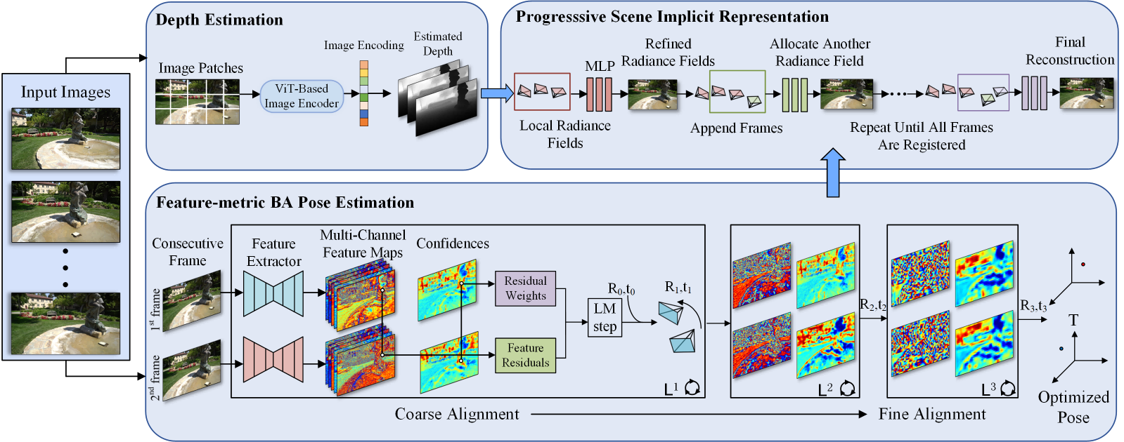
Figure 2: The pipeline of our system. There are three modules in our system: depth estimation module, FBA pose estimation module, and incremental scene implicit representation module. All three modules are jointly optimized during the system operation.

III-A Depth Estimation

In our depth network, we choose the vision transformer network as our backbone. Vision transformer network [45] has been proven to have strong feature learning capabilities. Most large vision models, such as Segment Anything Model [46], choose it as their backbone. Inspired by DPT [47], we leverage vision transformers in place of convolutional neural networks for dense depth prediction. We maintain an encoder-decoder structure for our depth network. For the input images $I\in H\times W\times 3$, these images are decomposed into a sequence of 2D patches, where $(H,W)$ is the height and width of the original image, $(P,P)$ is the resolution of each image patches. We use ResNet50 with group norm and weight standardization to encode these image patches. Our vision transformer module transforms these patches using sequential blocks of multi-headed self-attention (MSA).

$$\hat{Z}^{l}=MSA\left(LN\left(Z^{l-1}\right)\right)+Z^{l-1}$$ (1)

$$Z^{l}=MLP\left(LN\left(\hat{Z}^{l}\right)\right)+\hat{Z}^{l}$$

$$\hat{Z}^{l+1}=MSA\left(LN\left(Z^{l}\right)\right)+Z^{l}$$

$$Z^{l+1}=MLP\left(LN\left(\hat{Z}^{l+1}\right)\right)+\hat{Z}^{l+1},$$

where $Z^{l+1}$ is the output feature in stage $l$. LN represents layer norm operation. Then, we adopt a depth estimation head with a convolution layer and linear layer to decode the feature. The final linear layer projects this representation to a non-negative scalar that represents the inverse depth prediction for every pixel. Bilinear interpolation is used to upsample the representation. This depth network can provide dense and accurate depth predictions in large-scale scenes.

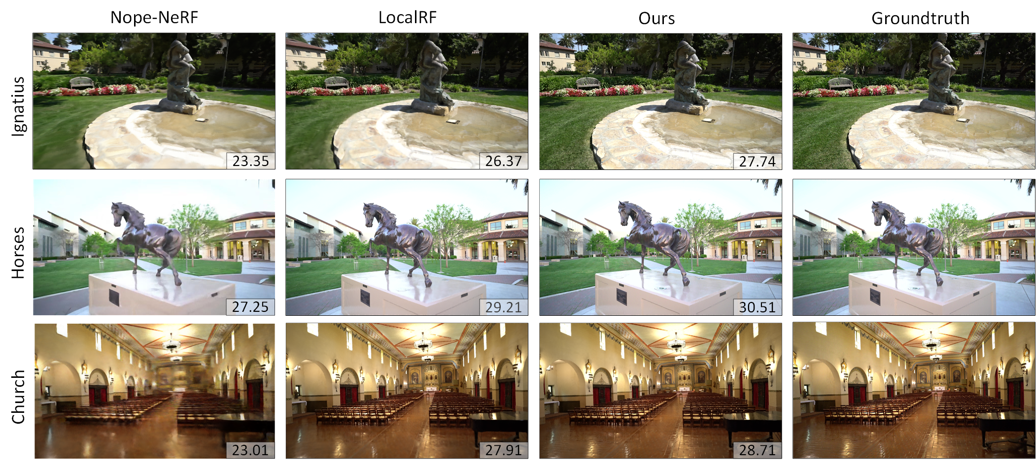
Figure 3: Qualitative results on Tanks and Temples datasets [21]. We present the scene reconstruction results of NoPe-NeRF[22], LocalRF [23], and our method with PSNR value. Our method performs better than other methods with higher-quality view synthesis results.

TABLE I: Novel view synthesis results on Tanks and Temples [21]. We use PSNR, SSIM, and LPIPS as our metrics.

Scenes		BARF [16]			NoPe-NeRF [22]			LocalRF [23]			Ours
		PSNR$\uparrow$	SSIM$\uparrow$	LPIPS$\downarrow$	PSNR$\uparrow$	SSIM$\uparrow$	LPIPS$\downarrow$	PSNR$\uparrow$	SSIM$\uparrow$	LPIPS$\downarrow$	PSNR$\uparrow$	SSIM$\uparrow$	LPIPS$\downarrow$
Tanks and Temples [21]	Ballroom	20.66	0.50	0.60	24.97	0.71	0.39	25.29	0.89	0.08	26.50	0.85	0.08
	Barn	25.28	0.64	0.48	25.77	0.68	0.44	27.89	0.88	0.11	28.59	0.91	0.11
	Church	23.17	0.62	0.52	23.60	0.67	0.46	28.07	0.91	0.07	28.82	0.92	0.08
	Family	23.04	0.61	0.56	23.77	0.68	0.48	28.60	0.92	0.007	30.48	0.94	0.05
	Francis	25.85	0.69	0.57	29.48	0.80	0.38	31.71	0.93	0.11	33.38	0.93	0.10
	Horse	24.09	0.72	0.41	27.30	0.83	0.27	29.98	0.94	0.07	30.07	0.93	0.07
	Ignatius	21.78	0.47	0.60	23.77	0.61	0.47	26.54	0.86	0.09	27.33	0.87	0.09
	Museum	23.58	0.61	0.55	26.39	0.76	0.36	26.35	0.86	0.16	29.43	0.92	0.12
	Mean	23.42	0.61	0.54	26.34	0.74	0.39	27.87	0.91	0.09	29.04	0.90	0.09

III-B Feature-metric BA Pose Estimation

In terms of pose estimation, we propose a FBA network. We show the architecture of our network in Fig. 2. Inspired by [48], each image is encoded into high-level features and uses FBA to get an accurate and robust pose estimation. For every consecutive frames $I_{a},I_{b}$, we use a Unet-like encoder-decoder network to extract $D_{l}$ dimensional feature map $\mathbf{F}^{l}\in\mathbb{R}^{W_{l}\times H_{l}\times D_{l}}$ at each level $l\in\{L,\ldots,1\}$. Those multi-channel image features with decreasing resolution can encode richer semantic information and larger spatial information of the image. Our network can also simultaneously estimate the confidence of each pixel to select the robust features for pose estimation.
Compared with the original BA method, this learned representation is robust to large illumination or viewpoint changes, which can provide accurate pose estimation in indoor and outdoor environments. Despite poor initial pose estimates, it can also provide meaningful gradients for successful estimation. Those joint learning methods with classical direct alignment [22, 23] operate on the original RGB image, which is not robust to large-scale scenes and long-term changes, and resorts to Gaussian image pyramids, which still largely limits the convergence to frame-to-frame tracking.
Feature Residual: We define the direct feature residual between the two consecutive frames. We optimize the relative pose$\{R,t\}$ through minimizing the feature residual. For a given feature level $l$ and each 3D point $i$ observed in two consecutive frames, we define a residual:

$$\mathbf{R}_{a}^{i}=\mathbf{F}_{b}^{l}\left[\Pi\left(\mathbf{R}\mathbf{P}_{i}+\mathbf{t}\right)_{b}\right]-\mathbf{F}_{a}^{l}\left[\mathbf{p}_{a}^{i}\right]$$ (2)

where $\Pi\left(\mathbf{R}\mathbf{P}_{i}+\mathbf{t}\right)_{b}$ is the projection of frame b given its current pose estimate. [·] is a lookup with sub-pixel interpolation. $F_{a}^{l},F_{b}^{l}$ are the corresponding feature maps of images a and b. The total error over N observations is:

$$E_{l}(\mathbf{R},\mathbf{t})=\sum_{i,a}w_{a}^{i}\rho\left(\left\|\mathbf{R}_{a}^{i}\right\|_{2}^{2}\right)$$ (3)

where $\rho(\cdot)$ is a robust cost function with derivative $\rho^{\prime}$, and $\omega_{a}^{i}$ is a per-residual weight. We use the Levenberg-Marquardt (LM) algorithm to iteratively optimize this nonlinear least-squares cost from an initial estimate. Follow [48], each pose update $\delta\in R$ is parametrized on the SE(3) manifold using its Lie algebra.

$$\boldsymbol{\delta}=-(\mathbf{H}+\lambda\operatorname{diag}(\mathbf{H}))^{-1}\mathbf{J}^{\top}\mathbf{Wr}$$ (4)

where $\lambda$ is the damping factor and H is the Hessian matrices. Then, the final pose can be defined by left-multiplication on the manifold.

Feature-metric BA loss: Our network is trained by minimizing the FBA of the corresponding pixel from coarse level to fine level:

$$\mathcal{L}_{FBA}=\frac{1}{L}\sum_{l}\sum_{i}\left\|\Pi\left(\mathbf{R}_{l}\mathbf{P}_{i}+\mathbf{t}_{l}\right)-\Pi\left(\overline{\mathbf{R}}\mathbf{P}_{i}+\overline{\mathbf{t}}\right)\right\|_{\gamma}$$ (5)

where $\gamma$ is the Huber cost. With coarse-to-fine pose estimation, low-resolution feature maps are responsible for the robustness of the pose estimation, while finer features enhance its accuracy. This feature-metric BA loss weights the supervision of the rotation and translation adaptively for each training example. It greatly enhances the accuracy and robustness of our pose network in large-scale scenes.

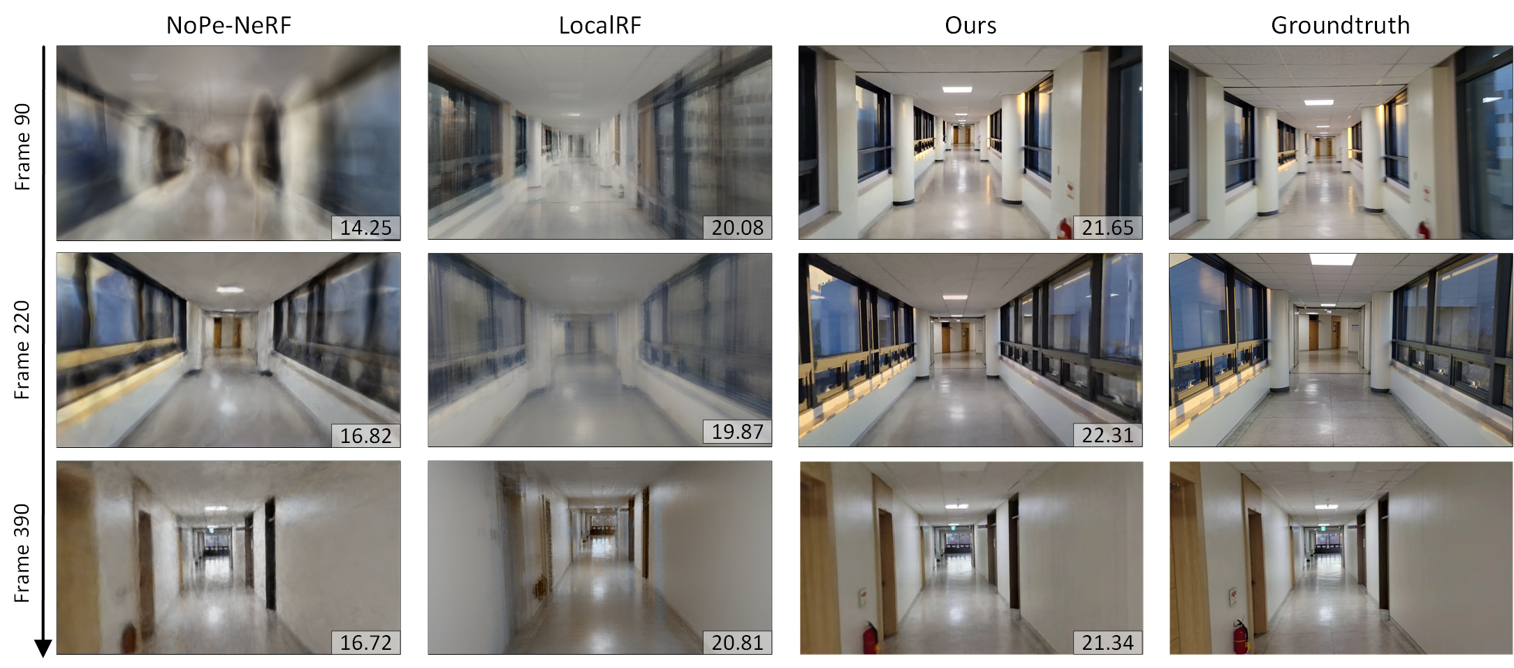
Figure 4: Qualitative results on Static Hikes Indoor datasets [23] with 40m trajectory and span over 1000 images. We present the scene reconstruction results of NoPe-NeRF[22], LocalRF [23], and our method in different time steps (90, 220, 390). Our incremental scene representation method significantly improves the scene reconstruction performance in large-scale scenes.

III-C Incremental Implicit Scene Representation

Existing scene implicit scene representation methods such as [17, 49, 16] can only achieve satisfactory results in small-scale scenes. They are frequently constrained by their limitations in scene representation capabilities when dealing with longer sequences and tend to converge towards local minima during the optimization process. Inspired by [23], we propose an incremental implicit scene representation. The architecture of our network is shown in Fig. 2. At the beginning, we will initialize a local neural radiance field and optimize it using the initial few frames as input. As the robot moves forward, we progressively append new frames within the local neural radiance field and iteratively refine the scene representation, pose estimation, and depth estimation. This procedure persists until we reach the boundary of the local neural radiance field. Then, we dynamically allocate new local radiance fields throughout the optimization with frames within a sliding window. This procedure will continue until all the images are registered into the network. So, the entire scene can be represented as multiple local NeRF:

$$\{I_{i},D_{i}\}_{i=1}^{M}\mapsto\{\mathrm{LR}^{1}_{\theta_{1}},\mathrm{LR}^{2}_{\theta_{2}},\dots,\mathrm{LR}^{n}_{\theta_{n}}\}\mapsto\{\mathbf{c},\mathbf{\sigma}\}$$ (6)

where $D_{i}$ is the estimated depth image from our depth network, $\mathbf{c}$ denotes the image color, $\sigma$ represents the volume density. Whenever the estimated camera pose exceeds the boundaries of the current local radiance fields, we cease optimizing previous poses and freeze the network parameters. This allows us to decrease memory usage by discarding supervisory frames that are no longer needed. During the optimization, we jointly optimize the depth, pose, and scene representation in the local radiance fields.

TABLE II: Pose estimation results on Tanks and Temples datasets [21]. We use ATE and RPE as our metrics.

Scenes		BARF [16]			NoPe-NeRF [22]			LocalRF [23]			Ours
		ATE$\downarrow$	RPEr$\downarrow$	RPEt$\downarrow$	ATE$\downarrow$	RPEr$\downarrow$	RPEt$\downarrow$	ATE$\downarrow$	RPEr$\downarrow$	RPEt$\downarrow$	ATE$\downarrow$	RPEr$\downarrow$	RPEt$\downarrow$
Tanks and Temples [21]	Ballroom	0.019	0.228	0.343	0.003	0.026	0.054	0.014	0.077	0.052	0.014	0.022	0.051
	Barn	0.075	0.326	1.402	0.023	0.034	0.127	0.019	0.088	0.048	0.019	0.015	0.044
	Church	0.059	0.063	0.458	0.026	0.013	0.088	0.017	0.077	0.042	0.016	0.023	0.111
	Family	0.116	0.595	0.577	0.006	0.045	0.049	0.004	0.074	0.043	0.004	0.021	0.035
	Francis	0.095	0.749	0.924	0.005	0.029	0.069	0.004	0.035	0.082	0.003	0.025	0.068
	Horse	0.016	0.399	0.239	0.005	0.032	0.192	0.037	0.287	0.561	0.014	0.027	0.035
	Ignatius	0.057	0.288	1.187	0.003	0.010	0.039	0.003	0.076	0.028	0.002	0.017	0.061
	Museum	0.257	1.128	2.589	0.035	0.247	0.335	0.025	0.303	0.179	0.025	0.219	0.217
	Mean	0.087	0.472	0.965	0.006	0.056	0.080	0.015	0.101	0.082	0.012	0.046	0.077

Differentiable Rendering For every input image $I$, we use the camera intrinsic matrix and camera pose to generate rays $r=x_{i}+td_{i}$. We sample points $x_{i}$ along rays. Then, we query our local radiance fields to get the color and density. $F_{\Theta}:(\mathbf{x_{i}},\mathbf{d_{i}})\rightarrow(\mathbf{c},\sigma)$. Through differentiable rendering, we can render along the rays:

$$\hat{\mathbf{C}}(\mathbf{r}) =\sum_{i=1}^{N}T_{i}\left(1-\exp\left(-\sigma_{i}\delta_{i}\right)\right)\mathbf{c}_{i},$$ (7)

$$T_{i} =\exp\left(-\sum_{i-1}^{j}\sigma_{j}\delta_{j}\right)$$

where $\delta_{i}$ is the distance between sample points and $T_{i}$ represents the accumulated transmittance along the ray. Compared with existing scene representation methods, we have re-parameterized the scene representation for unbounded scenes similar to [50]. We use a contract function to map every point into a cubic space:

$$\operatorname{contract}(\mathbf{x})=\begin{cases}\mathbf{x}&\text{ if }\|\mathbf{x}\|_{\infty}\leq 1\\ \left(2-\frac{1}{\|\mathbf{x}\|_{\infty}}\right)\left(\frac{\mathbf{x}}{\|\mathbf{x}\|_{\infty}}\right)&\text{ otherwise. }\end{cases}$$ (8)

This contract function can help our method to reconstruct unbounded scenes.

III-D Incremental Joint Learning

In this section, we provide more details of the optimization of depth $D$, RGB $C$, camera poses $\{R,t\}$, and scene representation $\theta$. In order to optimize our depth network and render depth images, we propose depth loss and estimated depth function.

$$\hat{\mathbf{D}}(\mathbf{r})=\sum_{i=1}^{N}T_{i}\left(1-\exp\left(-\sigma_{i}\delta_{i}\right)\right)d_{i}$$ (9)

$$\mathcal{L}_{d}=\left|\hat{\mathbf{D}}^{*}-\mathbf{D}^{*}\right|$$ (10)

where $\hat{D}^{*}(r)$ is our render depth, $D^{*}(r)$ is our estimated depth image from our depth network. We use a pre-trained model to get depth images prior to our depth network. We define a photo-metric loss to optimize local radiance fields:

$$\mathcal{L}_{p}=\|\hat{\mathbf{C}}(\mathbf{r})-\mathbf{C}(\mathbf{r})\|_{2}^{2}$$ (11)

where $\hat{C}(r)$ is the render image and $C(r)$ is the input RGB image. We also add an optical flow loss between neighbor frames as they have proven to improve the accuracy and robustness in challenging scenarios.

$$\hat{\mathcal{F}}_{k\rightarrow k+1}=(u,v)-\Pi\left(\{R,t\}_{k\rightarrow k+1}\Pi^{-1}(u,v,\hat{D})\right)$$ (12)

Where $\Pi^{-1}$ represents the back-projection from pixel coordinates into 3D points. $\{R,t\}_{k\rightarrow k+1}$ means the relative camera pose transformation. Then, we calculate our optical flow loss:

$$\mathcal{L}_{fa}=\left\|\hat{\mathcal{F}}_{k\rightarrow k+1}-\mathcal{F}_{k\rightarrow k+1}\right\|_{1}$$ (13)

This is the forward optical flow and we also calculate backward optical flow $L_{fb}$ to supervise our implicit scene representation network. The final loss of our network is :

$$\mathcal{L}=\lambda_{1}\mathcal{L}_{p}+\lambda_{2}\mathcal{L}_{D}+\lambda_{3}\mathcal{L}_{FBA}+\lambda_{4}\mathcal{L}_{fa}+\lambda_{5}\mathcal{L}_{fb}$$ (14)

We use the progressive optimization scheme to improve the robustness and to satisfy large-scale scenes and long sequences. We start by using a small amount of frames (for example five frames) to initiate the operation. Subsequently, we progressively introduce new frames into the optimization process in a sequential manner.

TABLE III: Novel view synthesis on Static Hikes dataset [23] and Proprietary dataset. We use PSNR, SSIM, and LPIPS as our metrics.

Methods	Static Hikes Indoor [23]						Proprietary Dataset
	PSNR$\uparrow$	SSIM$\uparrow$	LPIPS$\downarrow$	ATE$\downarrow$	RPEr$\downarrow$	RPEt$\downarrow$	PSNR$\uparrow$	SSIM$\uparrow$	LPIPS$\downarrow$	ATE$\downarrow$	RPEr$\downarrow$	RPEt$\downarrow$
BARF [16]	14.81	0.692	0.737	0.632	0.545	1.791	12.38	0.56	0.75	2.463	1.334	2.482
NoPe-NeRF [22]	16.82	0.74	0.62	0.463	0.443	1.595	20.17	0.68	0.56	0.970	0.140	1.459
LocalRF [23]	20.08	0.702	0.448	0.231	0.846	1.443	19.63	0.649	0.432	0.234	0.585	0.707
Ours	21.65	0.709	0.306	0.203	0.941	1.752	22.09	0.764	0.277	0.232	0.385	0.610

IV Experiments

In this section, we present our experimental results on different real-world datasets and conduct a comprehensive ablation study to verify the effectiveness of our method. We also gather proprietary real-world datasets using a robotic wheelchair to assess performance on mobile platforms in real-world applications.

Baselines Methods and Public Datasets. The main baseline methods we compared are BARF [16], NoPe-NeRF [22], and LocalRF [23]. All of them are joint learning methods of camera poses and implicit scene representation. We evaluate our method on the Tanks and Temples dataset [21] and Static Hikes dataset [23]. The Tanks and Temples dataset features slow-moving image sequences spanning a few meters in both indoor and outdoor scenes. We also utilize the Static Hikes indoor dataset, which includes hand-held sequences with longer camera trajectories, testing scalability and pose estimation robustness over ranges typically exceeding 30 meters. We strictly follow the experimental settings of our baseline to partition the training set and the test set.

Our Dataset. An in-house proprietary dataset was collected using an intelligent wheelchair to simulate the application of NeRF in elderly care settings, as shown in Fig. 5. The dataset includes a long-distance travel scene spanning over 35 meters and consists of over 1k images. Our intelligent wheelchair features two sensors: the Realsense D435i, an RGBD camera capturing only the RGB images, and the Robosense RS-Lidar-16, aimed at obtaining groundtruth poses with a certified performance at 2 cm level accuracy [51]. We evaluate the capabilities of our depth, pose estimation, and scene representation. We use this dataset to validate the performance of our method in real-world robot operations.

Figure 5: The image above is a prototype of our robot platform, and below are the qualitative results of our method on our own real-world datasets with PSNR value. We compare the view synthesis results with NoPe-NeRF[22], LocalRF [23]. Our method performs better on real-world datasets.

Figure 6: Qualitative results of depth estimation on Tanks and Temples datasets [21]. We present the depth estimation results of NoPe-NeRF[22], LocalRF [23], and our method. The region outlined on the image is marked in red and black to signify lower accuracy, in green to signify higher accuracy and groundtruth.

Implementation Details. We present our implementation details. We select Adam optimizer[52] ($\beta=(0.9,0.999)$) for scene representation and camera tracking optimization. The color loss weighting is $\lambda_{1}=0.25$, $\lambda_{2}=0.1$ for depth and $\lambda_{3}=1.0$ for pose estimation, $\lambda_{4}=1.0$, $\lambda_{5}=1.0$ for optical flow. All training and evaluation experiments are conducted on a single NVIDIA RTX 3090 GPU.

IV-A Experimental Results

In this section, we evaluate the system in different datasets ranging from indoor scenes to large outdoor scenes on Tanks and Temples [21], Static Hikes Indoor [23] and our dataset.

Scene Reconstruction Results. We use Peak Signal-to-noise Ratio (PSNR), Structural Similarity Index Measurement (SSIM), and Learned Perceptual Image Patch Similarity (LPIPS) to evaluate view synthesis results. In Table I, we present the scene reconstruction results on Tanks and Temples datasets. Our method outperforms all the baselines by a large margin. The scene reconstruction results on other datasets are shown in Table III. Our method outperforms other methods in scene representation. The incremental implicit scene representation method significantly enhances the scene representation ability and performs well on large-scale and long-sequence datasets. The qualitative results are shown in Fig. 3,4,5. In Fig. 3, We present the view synthesis results on different sequences Ignatius, Horses, Church in Tanks and Temples dataset [21]. Our method achieves higher-quality image reconstruction results. In Fig. 4, these images correspond to different timesteps (90,390,900) from up to down. We place the PSNR values of each scene in the bottom right corner. In contrast, our incremental scene representation method achieves high-quality view synthesis results compared with NoPe-NeRF and LocalRF. In Fig. 5, we show the image reconstruction results on our own dataset. Compared with other joint learning methods, our method achieves the most high-fidelity novel view results in both outdoor and indoor scenes.

Pose Estimation Results. The pose estimation results are shown in Table. II and Table. III. We use Absolute Trajectory Error (ATE), and Relative Pose Error (RPE) as the pose estimation metrics. Our pose estimation network performs better than other existing methods. The FBA method performs re-projection optimization in the high-dimensional feature level, which avoids various disturbances and noise present at the image level. The FBA network enhances the accuracy and robustness of the pose estimation in large-scale scenes. We also present the depth estimation results in Fig. 6. Compared to our method, a tree is missing from the LocalRF estimated depth, as shown in red blocks, and the depth at both bushes and trees in NoPe-NeRF is inaccurate, as shown in black blocks. Our estimated depth images are more accurate and sharper, as shown in green blocks.

Figure 7: Importance of incremental scene representation. We compare the scene reconstruction results with two types of radiance fields model (single, multiple) on Tanks and Temples dataset [21] and Static Hikes dataset [23]. In the first row, we use a single radiance field, which fails in large-scale scenes. In the second row, we use local radiance fields, which improve the representation capability and produce high-fidelity and sharper results.

TABLE IV: Ablation studies of different modules on Tanks and Temples datasets [21].

	Tanks and Temples [21]
	PSNR$\uparrow$	SSIM$\uparrow$	LPIPS$\downarrow$	ATE$\downarrow$	RPEr$\downarrow$	RPEt$\downarrow$
(a) w/o FBA-net	27.15	0.87	0.10	0.017	0.157	0.143
(b) w/o PO	25.87	0.84	0.15	0.016	0.152	0.141
(c) w/o $L_{d}$	26.75	0.86	0.11	0.017	0.143	0.137
Ours	29.11	0.90	0.09	0.013	0.139	0.133

IV-B Ablation Study

In this section, we conduct sufficient ablation studies to verify the effectiveness of our designed network. We show the ablation results in Table IV. (a) is the network without a FBA network. (b) is the network without progressive optimization. (c) is the network without depth loss. For the FBA network, we remove it in Table IV. (a), and replace it with traditional pose optimization. We can see that this network improves the accuracy of the pose estimation results. For the progressive optimization network, we replace it with global optimization. We can see that the progressive network significantly improves the scene representation and pose estimation. We also present the render results between using a single global radiance field and using multiple radiance fields in Fig. 7. This indicates the importance of our incremental scene representation method. In Table (c), we remove the depth loss and the depth network is not jointly optimized with other networks. The results indicate that the depth loss and joint optimization strategy are effective for scene representation and pose estimation.

V Conclusion

In this paper, we propose a novel incremental joint learning network of depth, pose, and implicit scene representation. The proposed FBA network extracts multi-level image features and performs coarse-to-fine BA estimation for corresponding pixels and image pose, which can provide accurate pose estimation results both in indoor and outdoor scenes. An incremental scene representation method is designed for large-scale scenes and long-sequence videos. This proposed network can achieve accurate and robust scene representation for arbitrarily long-sequence scene reconstruction. Compared with other joint learning methods, our method achieves SOTA results in depth estimation, pose estimation, and implicit scene representation in large-scale indoor and outdoor scenes.

References

- [1] X. Zhao, Q. Li, C. Wang, H. Dou, and B. Liu, “Robust depth-aided visual-inertial-wheel odometry for mobile robots,” IEEE Transactions on Industrial Electronics, 2023.
- [2] K. W. Tong, X. Y. Zhao, Y. X. Li, and P. Li, “Individual-level fmri segmentation based on graphs,” IEEE Transactions on Cognitive and Developmental Systems, vol. 15, no. 4, pp. 1773–1782, 2023.
- [3] Z. Zheng, S. Lin, and C. Yang, “Rld-slam: A robust lightweight vi-slam for dynamic environments leveraging semantics and motion information,” IEEE Transactions on Industrial Electronics, 2024.
- [4] K. W. Tong, J. Wu, and Y. H. Hou, “Robust drogue positioning system based on detection and tracking for autonomous aerial refueling of uavs,” IEEE Transactions on Automation Science and Engineering, 2023, early access, doi: 10.1109/TASE.2023.3308230. .
- [5] T. Liu, Q. Cai, C. Xu, B. Hong, J. Xiong, Y. Qiao, and T. Yang, “Image captioning in news report scenario,” Academic Journal of Science and Technology, vol. 10, no. 1, pp. 284–289, 2024.
- [6] X. Wang, Y. Qiao, J. Xiong, Z. Zhao, N. Zhang, M. Feng, and C. Jiang, “Advanced network intrusion detection with tabtransformer,” Journal of Theory and Practice of Engineering Science, vol. 4, no. 03, pp. 191–198, 2024.
- [7] C. Wu, Z. Gong, B. Tao, K. Tan, Z. Gu, and Z. Yin, “Rf-slam: Uhf-rfid based simultaneous tags mapping and robot localization algorithm for smart warehouse position service,” IEEE Transactions on Industrial Informatics, 2023.
- [8] W. Tong, X. Guan, J. Kang, P. Z. H. Sun, R. Law, P. Ghamisi, and E. Q. Wu, “Normal assisted pixel-visibility learning with cost aggregation for multiview stereo,” IEEE Transactions on Intelligent Transportation Systems, vol. 23, no. 12, pp. 24 686–24 697, 2022.
- [9] K. W. Tong, P. Z. H. S. andE. Q. Wu, C. Wu, and Z. Jiang, “Adaptive cost volume representation for unsupervised high-resolution stereo matching,” IEEE Transactions on Intelligent Vehicles, vol. 8, no. 1, pp. 912–922, 2023.
- [10] W. Tong, X. Guan, M. Zhang, P. Li, J. Ma, E. Q. Wu, and L.-M. Zhu, “Edge-assisted epipolar transformer for industrial scene reconstruction,” IEEE Transactions on Automation Science and Engineering, 2024, early access, doi: 10.1109/TASE.2023.3330704. .
- [11] B. Mildenhall, P. P. Srinivasan, M. Tancik, J. T. Barron, R. Ramamoorthi, and R. Ng, “Nerf: Representing scenes as neural radiance fields for view synthesis,” Communications of the ACM, vol. 65, no. 1, pp. 99–106, 2021.
- [12] T. Deng, H. Xie, J. Wang, and W. Chen, “Long-term visual simultaneous localization and mapping: Using a bayesian persistence filter-based global map prediction,” IEEE Robotics & Automation Magazine, vol. 30, DOI 10.1109/MRA.2022.3228492, no. 1, pp. 36–49, 2023.
- [13] Y. Deng, M. Wang, Y. Yang, D. Wang, and Y. Yue, “See-csom: Sharp-edged and efficient continuous semantic occupancy mapping for mobile robots,” IEEE Transactions on Industrial Electronics, vol. 71, DOI 10.1109/TIE.2023.3262857, no. 2, pp. 1718–1728, 2024.
- [14] J. Liu, G. Wang, C. Jiang, Z. Liu, and H. Wang, “Translo: A window-based masked point transformer framework for large-scale lidar odometry,” in Proceedings of the AAAI Conference on Artificial Intelligence, vol. 37, no. 2, pp. 1683–1691, 2023.
- [15] J. Liu, G. Wang, Z. Liu, C. Jiang, M. Pollefeys, and H. Wang, “Regformer: An efficient projection-aware transformer network for large-scale point cloud registration,” in Proceedings of the IEEE/CVF International Conference on Computer Vision (ICCV), pp. 8451–8460, Oct. 2023.
- [16] C.-H. Lin, W.-C. Ma, A. Torralba, and S. Lucey, “Barf: Bundle-adjusting neural radiance fields,” in Proceedings of the IEEE/CVF International Conference on Computer Vision (ICCV), pp. 5741–5751, Oct. 2021.
- [17] Y. Jeong, S. Ahn, C. Choy, A. Anandkumar, M. Cho, and J. Park, “Self-calibrating neural radiance fields,” in Proceedings of the IEEE/CVF International Conference on Computer Vision, pp. 5846–5854, 2021.
- [18] T. Deng, G. Shen, T. Qin, J. Wang, W. Zhao, J. Wang, D. Wang, and W. Chen, “Plgslam: Progressive neural scene represenation with local to global bundle adjustment,” arXiv preprint arXiv:2312.09866, 2023.
- [19] T. Deng, Y. Chen, L. Zhang, J. Yang, S. Yuan, D. Wang, and W. Chen, “Compact 3d gaussian splatting for dense visual slam,” arXiv preprint arXiv:2403.11247, 2024.
- [20] T. Deng, Y. Wang, H. Xie, H. Wang, J. Wang, D. Wang, and W. Chen, “Neslam: Neural implicit mapping and self-supervised feature tracking with depth completion and denoising,” arXiv preprint arXiv:2403.20034, 2024.
- [21] A. Knapitsch, J. Park, Q.-Y. Zhou, and V. Koltun, “Tanks and temples: Benchmarking large-scale scene reconstruction,” ACM Transactions on Graphics (ToG), vol. 36, no. 4, pp. 1–13, 2017.
- [22] W. Bian, Z. Wang, K. Li, J.-W. Bian, and V. A. Prisacariu, “Nope-nerf: Optimising neural radiance field with no pose prior,” in Proceedings of the IEEE/CVF Conference on Computer Vision and Pattern Recognition, pp. 4160–4169, 2023.
- [23] A. Meuleman, Y.-L. Liu, C. Gao, J.-B. Huang, C. Kim, M. H. Kim, and J. Kopf, “Progressively optimized local radiance fields for robust view synthesis,” in Proceedings of the IEEE/CVF Conference on Computer Vision and Pattern Recognition, pp. 16 539–16 548, 2023.
- [24] A. Roy and S. Todorovic, “Monocular depth estimation using neural regression forest,” in Proceedings of the IEEE conference on computer vision and pattern recognition, pp. 5506–5514, 2016.
- [25] N. Mayer, E. Ilg, P. Fischer, C. Hazirbas, D. Cremers, A. Dosovitskiy, and T. Brox, “What makes good synthetic training data for learning disparity and optical flow estimation?” International Journal of Computer Vision, vol. 126, pp. 942–960, 2018.
- [26] Z. Chen, L. Jing, L. Yang, Y. Li, and B. Li, “Class-level confidence based 3d semi-supervised learning,” in Proceedings of the IEEE/CVF Winter Conference on Applications of Computer Vision, pp. 633–642, 2023.
- [27] Z. Chen, L. Jing, Y. Liang, Y. Tian, and B. Li, “Multimodal semi-supervised learning for 3d objects,” arXiv preprint arXiv:2110.11601, 2021.
- [28] Z. Chen, L. Jing, Y. Li, and B. Li, “Bridging the domain gap: Self-supervised 3d scene understanding with foundation models,” Advances in Neural Information Processing Systems, vol. 36, 2024.
- [29] Z. Chen, Y. Li, L. Jing, L. Yang, and B. Li, “Point cloud self-supervised learning via 3d to multi-view masked autoencoder,” arXiv preprint arXiv:2311.10887, 2023.
- [30] C. Godard, O. Mac Aodha, and G. J. Brostow, “Unsupervised monocular depth estimation with left-right consistency,” in Proceedings of the IEEE conference on computer vision and pattern recognition, pp. 270–279, 2017.
- [31] J.-W. Bian, H. Zhan, N. Wang, Z. Li, L. Zhang, C. Shen, M.-M. Cheng, and I. Reid, “Unsupervised scale-consistent depth learning from video,” International Journal of Computer Vision, vol. 129, no. 9, pp. 2548–2564, 2021.
- [32] R. Garg, N. Wadhwa, S. Ansari, and J. T. Barron, “Learning single camera depth estimation using dual-pixels,” in Proceedings of the IEEE/CVF international conference on computer vision, pp. 7628–7637, 2019.
- [33] T. Deng, S. Liu, X. Wang, Y. Liu, D. Wang, and W. Chen, “Prosgnerf: Progressive dynamic neural scene graph with frequency modulated auto-encoder in urban scenes,” arXiv preprint arXiv:2312.09076, 2023.
- [34] W. He, Z. Jiang, C. Zhang, and A. M. Sainju, “Curvanet: Geometric deep learning based on directional curvature for 3d shape analysis,” in Proceedings of the 26th ACM SIGKDD International Conference on Knowledge Discovery & Data Mining, pp. 2214–2224, 2020.
- [35] W. He, A. M. Sainju, Z. Jiang, and D. Yan, “Deep neural network for 3d surface segmentation based on contour tree hierarchy,” in Proceedings of the 2021 SIAM International Conference on Data Mining (SDM), pp. 253–261. SIAM, 2021.
- [36] T. Liu, Q. Cai, C. Xu, B. Hong, F. Ni, Y. Qiao, and T. Yang, “Rumor detection with a novel graph neural network approach,” Academic Journal of Science and Technology, vol. 10, no. 1, pp. 305–310, 2024.
- [37] H. Xie, T. Deng, J. Wang, and W. Chen, “Robust incremental long-term visual topological localization in changing environments,” IEEE Transactions on Instrumentation and Measurement, vol. 72, pp. 1–14, 2022.
- [38] H. Xie, T. Deng, J. Wang, and W. Chen, “Angular tracking consistency guided fast feature association for visual-inertial slam,” IEEE Transactions on Instrumentation and Measurement, 2024.
- [39] T. Liu, C. Xu, Y. Qiao, C. Jiang, and J. Yu, “Particle filter slam for vehicle localization,” Journal of Industrial Engineering and Applied Science, vol. 2, no. 1, pp. 27–31, 2024.
- [40] L. Yen-Chen, P. Florence, J. T. Barron, A. Rodriguez, P. Isola, and T.-Y. Lin, “inerf: Inverting neural radiance fields for pose estimation,” in 2021 IEEE/RSJ International Conference on Intelligent Robots and Systems (IROS), pp. 1323–1330. IEEE, 2021.
- [41] S. Zhu, G. Wang, H. Blum, J. Liu, L. Song, M. Pollefeys, and H. Wang, “Sni-slam: Semantic neural implicit slam,” arXiv preprint arXiv:2311.11016, 2023.
- [42] S. Zhu, R. Qin, G. Wang, J. Liu, and H. Wang, “Semgauss-slam: Dense semantic gaussian splatting slam,” arXiv preprint arXiv:2403.07494, 2024.
- [43] M. Li, S. Liu, and H. Zhou, “Sgs-slam: Semantic gaussian splatting for neural dense slam,” arXiv preprint arXiv:2402.03246, 2024.
- [44] M. Li, J. He, G. Jiang, and H. Wang, “Ddn-slam: Real-time dense dynamic neural implicit slam with joint semantic encoding,” arXiv preprint arXiv:2401.01545, 2024.
- [45] A. Dosovitskiy, L. Beyer, A. Kolesnikov, D. Weissenborn, X. Zhai, T. Unterthiner, M. Dehghani, M. Minderer, G. Heigold, S. Gelly et al., “An image is worth 16x16 words: Transformers for image recognition at scale,” arXiv preprint arXiv:2010.11929, 2020.
- [46] A. Kirillov, E. Mintun, N. Ravi, H. Mao, C. Rolland, L. Gustafson, T. Xiao, S. Whitehead, A. C. Berg, W.-Y. Lo et al., “Segment anything,” arXiv preprint arXiv:2304.02643, 2023.
- [47] R. Ranftl, A. Bochkovskiy, and V. Koltun, “Vision transformers for dense prediction,” in Proceedings of the IEEE/CVF International Conference on Computer Vision (ICCV), pp. 12 179–12 188, Oct. 2021.
- [48] P.-E. Sarlin, A. Unagar, M. Larsson, H. Germain, C. Toft, V. Larsson, M. Pollefeys, V. Lepetit, L. Hammarstrand, F. Kahl et al., “Back to the feature: Learning robust camera localization from pixels to pose,” in Proceedings of the IEEE/CVF conference on computer vision and pattern recognition, pp. 3247–3257, 2021.
- [49] Z. Wang, S. Wu, W. Xie, M. Chen, and V. A. Prisacariu, “Nerf–: Neural radiance fields without known camera parameters,” arXiv preprint arXiv:2102.07064, 2021.
- [50] J. T. Barron, B. Mildenhall, D. Verbin, P. P. Srinivasan, and P. Hedman, “Mip-nerf 360: Unbounded anti-aliased neural radiance fields,” in Proceedings of the IEEE/CVF Conference on Computer Vision and Pattern Recognition, pp. 5470–5479, 2022.
- [51] T.-M. Nguyen, D. Duberg, P. Jensfelt, S. Yuan, and L. Xie, “Slict: Multi-input multi-scale surfel-based lidar-inertial continuous-time odometry and mapping,” IEEE Robotics and Automation Letters, vol. 8, no. 4, pp. 2102–2109, 2023.
- [52] D. P. Kingma and J. Ba, “Adam: A method for stochastic optimization,” in Proceedings of the International Conference on Learning Representations, 2015.