Quantum computing topological invariants of two-dimensional quantum matter

Abstract

Quantum algorithms provide a potential strategy for solving computational problems that are intractable by classical means. Computing the topological invariants of topological matter is one central problem in research on quantum materials, and a variety of numerical approaches for this purpose have been developed. However, the complexity of quantum many-body Hamiltonians makes calculations of topological invariants challenging for interacting systems. Here, we present two quantum circuits for calculating Chern numbers of two-dimensional quantum matter on quantum computers. Both circuits combine a gate-based adiabatic time-evolution over the discretized Brillouin zone with particular phase estimation techniques. The first algorithm uses many qubits, and we analyze it using a tensor-network simulator of quantum circuits. The second circuit uses fewer qubits, and we implement it experimentally on a quantum computer based on superconducting qubits. Our results establish a method for computing topological invariants with quantum circuits, taking a step towards characterizing interacting topological quantum matter using quantum computers.

I Introduction

Classifying topological phases of matter is a central problem in modern condensed matter physics.Qi and Zhang (2011); Hasan and Kane (2010); Moessner and Moore (2021); J. Asbóth and Pályi (2016); Xiao et al. (2010); Ren et al. (2016) In recent years, it has been realized that topological matter harbors a range of exotic phenomena, including the existence of chiral edge statesChang et al. (2023) and helical modes,Maciejko et al. (2011) as well as fractional excitations and Majorana fermions.Alicea (2012) Topological phases of matter may be characterized by topological invariants, such as the Berry phase in one dimension Berry (1984); Zak (1989) and the Chern number in two dimensions, Fig. 1(a).Haldane (1988); Kane and Mele (2005) Ultimately, it is expected that certain topological excitations will make it possible to build a topological quantum computer that will be protected against the errors that limit current quantum processors. Kitaev (2001); Alicea et al. (2011); Nayak et al. (2008); Lahtinen and Pachos (2017)

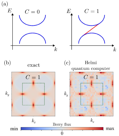
Figure 1: Quantum computations of topological invariants. (a) Two-dimensional quantum matter can be characterized by the Chern number $C$. A non-zero Chern number implies that edge states exist as indicated by a red line. (b,c) A quantum circuit can be used to calculate the Berry flux and the Chern number. The two panels show a comparison between exact results for the Berry flux in the extended Brillouin zone and actual calculations on the quantum computer Helmi.

Computational methods have been successful in predicting the topological phases of matter that can be described by single-particle Hamiltonians.T. Fukui and Suzuki (2005); K. Kudo and Hatsugai (2019) However, for strongly-correlated topological matter, where interactions may be important, the required computational resources scale exponentially with the system size, making it hard to predict their topological phase diagram. Variational eigensolvers implemented on quantum computers provide one promising strategy to characterize strongly-correlated quantum matter.Ayral et al. (2023) As such, quantum circuits for computing topological invariants of quantum matter have become a vibrant area of research.B. Murta and Fernández-Rossier (2020); Semeghini et al. (2021); X. Xiao and Kemper (2021, 2023); Sugimoto (2023); Mei et al. (2020); Smith et al. (2022); Azses et al. (2020); K. Choo and Neupert (2018); Roushan et al. (2014); Flurin et al. (2017); Xu et al. (2018); Zhan et al. (2017); R.-Y. Sun and Yunoki (2023)

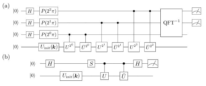
Figure 2: Quantum circuits for calculating Berry phases and fluxes. (a) The operator $U_{\text{init}}(\bm{k})$ initializes the lowest qubit followed by consecutive applications of the time-evolution operators, $U=U(T,0)$ and $\bar{U}=\bar{U}(T,0)$, defined in connection with Eq. (6). The first three qubits are used to read out the Berry phase with the quantum phase estimation algorithm. Hadamard gates are denoted by $H$, while $P(\varphi)$ are phase-shift gates. The inverse quantum Fourier transform is denoted as QFT^-1. (b) Quantum circuit with two qubits for reading out the Berry fluxes using a Hadamard test. Here, the adiabatic time-evolution operators only have to be applied once. The $S$-gate determines if the Berry flux should be determined using a sine or cosine function.

In this work, we present two quantum circuits for calculating the Chern number of two-dimensional quantum matter.B. Murta and Fernández-Rossier (2020); X. Xiao and Kemper (2023) The first circuit uses the quantum phase estimation algorithm to extract the Chern number from the winding of the Wannier center across the unit cell. This circuit typically requires many qubits, and we analyze it using a tensor-network simulator of quantum circuits. The second circuit exploits that the Chern number can be calculated by summing up the local Berry fluxes in momentum space, which can be determined using a Hadamard test algorithm. This circuit only requires a single auxiliary qubit, and we implement it using the quantum computer Helmi.Hel (2024a) As seen in Fig. 1(b,c), we find good agreement between our quantum computations and exact results for the Berry flux. As such, we show how quantum circuits make it possible to determine topological invariants of quantum matter, providing a promising starting point for characterizing strongly-correlated quantum matter using quantum computers.

The rest of this paper is organized as follows. In Sec. II, we introduce the two quantum circuits that we use to compute the Berry phase and the Chern numbers. We also describe the quantum computer and the tensor-network simulator of quantum circuits that we use for our calculations. In Sec. III, we present our results for the topological classification of the Qi-Wu-Zhang (QWZ) model and the Haldane model. Finally, in Sec. IV, we present our conclusions together with a brief outlook on possible avenues for future developments.

II Methods

II.1 Berry phase calculations

We first show how the Berry phase emerges from a Bloch Hamiltonian $H(\bm{k})$ that depends on the momentum $\bm{k}$. For each momentum, the Hamiltonian has a complete set of eigenstates denoted by $\{\ket{n(\bm{k})}\}$ with

$$H(\bm{k})\ket{n(\bm{k})}=E_{n}(\bm{k})\ket{n(\bm{k})}.$$ (1)

We now initialize the system in the eigenstate $\ket{n(\bm{k})}$ and let it evolve while changing the momentum in a closed loop from its initial value $\bm{k}(t=0)=\bm{k}$ to the final value $\bm{k}(t=T)=\bm{k}$. Moreover, we change the Hamiltonian slowly enough that the system remains in its instantaneous eigenstate $\ket{n(\bm{k}(t))}$ at all times, up to an overall phase factor. We can therefore write

$$U(T,0)\ket{n(\bm{k})}=e^{i(\Theta_{B}-\Theta_{D})}\ket{n(\bm{k})},$$ (2)

where

$$U(T,0)=\mathcal{T}\{e^{-i\int_{0}^{T}dtH(\bm{k}(t))}\}$$ (3)

is the time-evolution operator. According to the adiabatic theorem, the total phase that is picked up is given by the difference between the Berry phase,

$$\Theta_{B}=i\int_{0}^{T}dt\langle n(\bm{k}(t))|\partial_{t}|n(\bm{k}(t))\rangle,$$ (4)

and the dynamical phase,

$$\Theta_{D}=\int_{0}^{T}dtE_{n}(\bm{k}(t)).$$ (5)

If we condition $U(T,0)$ on an auxiliary qubit, the overall phase $\Theta_{B}-\Theta_{D}$ can be measured using a Hadamard test Luongo (2023) or the quantum phase estimation algorithm.Kitaev (1995); Nielsen and Chuang (2010)

In the following, we wish to determine the Berry phase $\Theta_{B}$ only. To this end, we let the system evolve through the same closed loop in momentum space one more time. However, we now let the system evolve backwards in time and denote the corresponding time-evolution operator by $\bar{U}(T,0)$. It is defined as in Eq. (3), however, with the opposite sign in the exponent. One may equivalently think of this unitary operator as propagating the system forward in time, but with the opposite sign of the Hamiltonian. We then easily see that the dynamical phase in Eq. (5) changes sign, since the eigenvalues change sign, while the Berry phase remains the same, since the eigenvectors are unchanged. After having traversed the closed loop twice, we therefore find

$$\bar{U}(T,0)U(T,0)\ket{n(\bm{k})}=e^{i2\Theta_{B}}\ket{n(\bm{k})},$$ (6)

which allows us to determine the Berry phase only.

Figure 2 shows the two quantum circuits for determining the Berry phase. The first circuit extracts the Berry phase using a quantum phase estimation algorithm. Typically, this circuit requires many qubits, so in the following we only simulate it using the tensor-network simulator that we describe below. The second circuit instead uses a Hadamard test to extract the Berry phase. This circuit requires fewer qubits, and we can implement it experimentally on a current quantum computer. In both circuits, we realize the time-evolution operators by a sequence of small time steps, B. Murta and Fernández-Rossier (2020) such that

$$U(T,0)\simeq\prod_{j=1}^{N}e^{-iH(\bm{k}(j\Delta t))\Delta t},$$ (7)

where $N$ is the number of time steps of length $\Delta t$ with $N\Delta t=T$, with an equivalent expression for $\bar{U}(T,0)$.

To check the output of the quantum circuits, we can also calculate the exact values of the Berry phase using the conventional Wilson-loop algorithm.Marzari and Vanderbilt (1997); Coh and Vanderbilt (2009); Wu et al. (2018); Yu et al. (2011); Gresch et al. (2017); Soluyanov and Vanderbilt (2011) Thus, we discretize a closed loop in momentum space as $\{\bm{k}_{1},\bm{k}_{2},...,\bm{k}_{N},\bm{k}_{1}\}$, assuming a non-degenerate ground state, and the Berry phase then reads

$$\Theta_{B}=\text{arg}\left[M_{\bm{k}_{1},\bm{k}_{2}}M_{\bm{k}_{2},\bm{k}_{3}}...M_{\bm{k}_{N},\bm{k}_{1}}\right],$$ (8)

where we have defined the overlaps of eigenstates as

$$M_{\bm{k}_{\alpha},\bm{k}_{\beta}}=\innerproduct{n(\bm{k}_{\alpha})}{n(\bm{k}_{\beta})}.$$ (9)

II.2 Chern number calculations

In the following, we use the quantum circuits from above to compute the Chern number of two-dimensional systems. For the circuit in Fig. 2(a), we use the fact that the Berry phase directly yields the positions of the hybrid Wannier centers, defined below, and we can then determine the Chern number directly from their winding across the unit cell.Marzari and Vanderbilt (1997); Coh and Vanderbilt (2009); Wu et al. (2018); Yu et al. (2011); Gresch et al. (2017); Soluyanov and Vanderbilt (2011) For the circuit in Fig. 2(b), we extract the Chern number from a direct calculation of the Berry flux in momentum space.Chang et al. (2023) For the circuit in Fig. 2(a), we need the quantum phase estimation algorithm to accurately determine the Berry phase, which is sizeable. By contrast, the circuit in Fig. 2(b) only relies on the extraction of small Berry phases in momentum space, and that can be done using a Hadamard test.

For the circuit in Fig. 2(a), we first show how the Chern number can be extracted from the winding number of a hybrid Wannier function. For a set Bloch functions $\ket{n(\bm{k})}$, the Wannier center is defined as

$$\bm{R}_{W}=\innerproduct{w_{n}(\bm{0})}{\bm{R}\,|w_{n}(\bm{0})}$$ (10)

in terms of the Wannier functions

$$\ket{w_{n}(\bm{R})}=\frac{1}{2\pi}\int_{BZ}d^{2}\bm{k}\,e^{i\bm{k}\cdot\bm{R}}\ket{n(\bm{k})}$$ (11)

evaluated at $\bm{R}=\bm{0}$. We can also define hybrid Wannier functions by keeping one of the momenta fixed and integrating over the other momentum. The center of the hybrid Wannier function in the $x$-coordinate as a function of $k_{y}$ is then given by

$$X_{W}(k_{y})=i\int_{-\pi}^{\pi}dk_{x}\innerproduct{n(\bm{k})}{\partial_{k_{x}}|n(\bm{k})}/2\pi.$$ (12)

By comparing this expression with Eq. (4), we see that the Wannier center is equal to the Berry phase, $X_{W}(k_{y})={\Theta_{B}}(k_{y})$, through a change of variables. Thus, the hybrid Wannier center can be obtained from the momentum-dependent Berry phase $\Theta_{B}(k_{y})$ by performing the adiabatic evolution over $k_{x}$ from $-\pi$ to $\pi$. By counting the number of times the center $X_{W}$ winds around the unit cell, we find the Chern number.Marzari and Vanderbilt (1997); Coh and Vanderbilt (2009); Wu et al. (2018); Yu et al. (2011); Gresch et al. (2017); Soluyanov and Vanderbilt (2011)

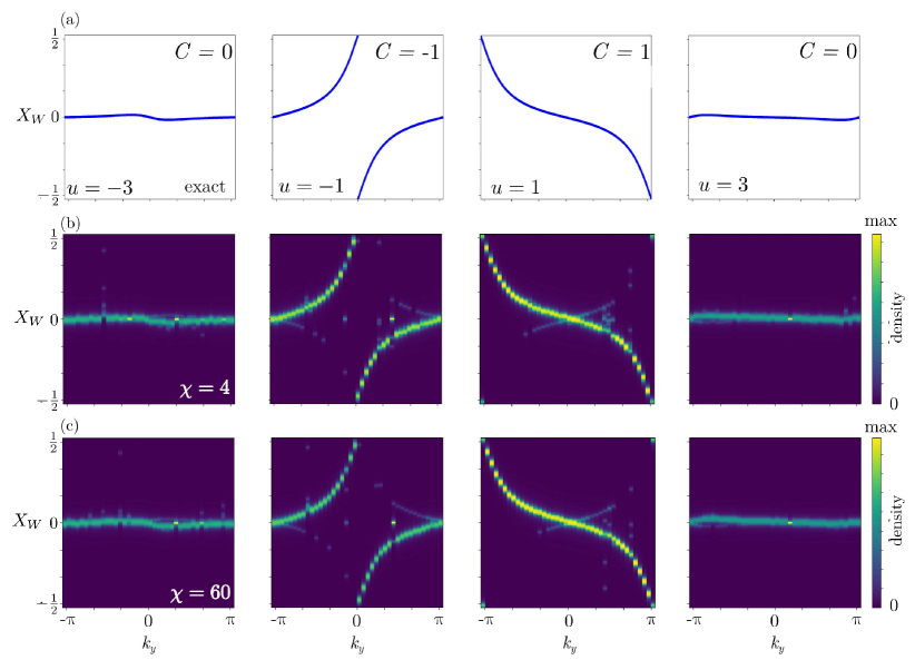
Figure 3: Wannier centers of the QWZ model. Results are shown for different values of the on-site potential, $u=-3,-1,1,3$, corresponding to different topological phases. (a) Exact calculations of the Wannier centers $X_{W}$ together with the Chern numbers that are extracted from the winding across the Brillouin zone. (b) Tensor-network simulation of the quantum circuit in Fig. 2(a) with a maximum bond dimension of $\chi=4$. (c) Similar simulations with a maximum bond dimension of $\chi=60$.

For the circuit in Fig. 2(b), we calculate the Chern number directly by integrating over the Berry flux. The Chern number is defined as the integral

$$C=\frac{1}{2\pi}\int_{BZ}d^{2}\bm{k}\Omega(\bm{k}),$$ (13)

where the Berry curvature,

$$\Omega(\bm{k})=\partial_{k_{x}}A_{k_{y}}-\partial_{k_{y}}A_{k_{x}},$$ (14)

is defined as the curl of the Berry connection

$$\bm{A}=i\langle n(\bm{k})|\nabla_{\bm{k}}|n(\bm{k})\rangle.$$ (15)

To calculate the Chern number, we decompose the Brillouin zone into $N\times N$ plaquettes of size $(\Delta k)^{2}$, such that $\Delta k=2\pi/N$. The Chern number is then

$$C\simeq\frac{1}{2\pi}\sum_{i,j=1}^{N}\Omega_{ij},$$ (16)

where $\Omega_{ij}$ is the Berry flux through the plaquette at position $(i,j)$ in the Brillouin zone. This flux can be computed as the Berry phase accumulated during an adiabatic evolution around the plaquette T. Fukui and Suzuki (2005) given by the loop

$$\begin{split}(k_{x},k_{y})&\rightarrow(k_{x}+\Delta k,k_{y})\rightarrow(k_{x}+\Delta k,k_{y}+\Delta k)\\ &\rightarrow(k_{x},k_{y}+\Delta k)\rightarrow(k_{x},k_{y}).\end{split}$$ (17)

Repeating this procedure for every plaquette and summing up the resulting Berry fluxes, we then find the Chern number according to Eq. (16). For small plaquettes, the associated Berry flux is small enough, typically below $10^{-2}$, that we can apply the Hadamard test algorithm to read out the Berry phase at the end of each adiabatic evolution. For this approach, the preparation of the eigenstate $\ket{n(\bm{k})}$ is only required once per plaquette. For our calculations, we prepare the initial state $\ket{n(\bm{k})}$ using the similarity transformation $U_{\text{init}}(\bm{k})$ that diagonalizes the Hamiltonian. By contrast, more complicated systems might require a ground-state preparation based on a variational quantum eigensolver for instance.Tilly et al. (2022)

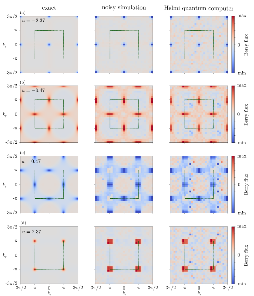
Figure 4: Berry flux of the QWZ model. The extended Brillouin zone is divided into $15\times 15$ plaquettes, while the first Brillouin zone is indicated by a dashed square. From left to right, we show exact results, results from noisy simulations, and results from Helmi. The rows correspond to different on-site potentials $u$. These results are used to find the Chern numbers in Fig. 5.

II.3 Quantum computations and tensor-network simulations

We implement our quantum circuit calculations on the Helmi quantum computer.Hel (2024a) Helmi is a 5-qubit quantum computer based on superconducting qubits, which are connected in a star-shaped topology. Its native quantum gates are the controlled-$Z$ gate and the one-qubit phased rotation gate around the $x$-axis, and it can be steered with standard Qiskit instructions. Helmi’s $T_{1}$ and $T_{2}$ times are $35.7$ $\mu$s and $17.4$ $\mu$s with a one- and two-qubit native gate application time of $120$ ns, allowing for a circuit depth of about $170$ native gates before qubit decoherence becomes an issue. Typical one- and two-qubit gate fidelities are $99.6$ $\%$ and $96.1$ $\%$, respectively. An important parameter for our circuit implementations is the optimization level of the transpilation to the quantum processor. Here we always use the highest possible level, which is level $3$. We also perform noisy simulations of Helmi with the fake backend FakeAdonis().

The circuit in Fig. 2(a) produces large Berry phases, and we therefore need to use the quantum phase estimation algorithm, instead of a Hadamard test. For this reason, the circuit requires more qubits, and it cannot be implemented on the Helmi quantum computer currently. Instead, we simulate this quantum circuit using matrix product states, which are a subclass of tensor networks.Schollwöck (2011)

Using matrix product states, a generic quantum state

$$\ket{\Psi}=\sum_{\bm{\sigma}}\Gamma^{\bm{s}}|\bm{s}\rangle$$ (18)

can be represented by the tensor train

$$\Gamma^{\bm{s}}=\sum_{{\bm{s}}}[A_{1}]_{\chi_{1}}^{s_{1}}[A_{2}]_{\chi_{1}\chi_{2}}^{s_{2}}...[A_{N}]_{\chi_{N-1}}^{s_{N}},$$ (19)

where $\{\ket{\bm{s}}\}$ are the computational basis states. The size of each tensor, $A_{i}$, is controlled by the bond dimension $\chi_{i}$. Thus, by adjusting the maximum bond dimension, an upper bound on the entanglement in a quantum state can be imposed. As such, we can simulate the generic loss of entanglement in a quantum computer by reducing the bond dimension.Niedermeier et al. (2023); Zhou et al. (2020); Stoudenmire and Waintal (2023); Ayral et al. (2023); Wang et al. (2017); Dang et al. (2019); Woolfe et al. (2017) Here, our tensor-network simulations are performed using the ITensors package,Fishman et al. (2022) interfaced to our publicly available quantum circuit simulation package called Quantunity.Niedermeier (2024)

III Results

III.1 Qi-Wu-Zhang model

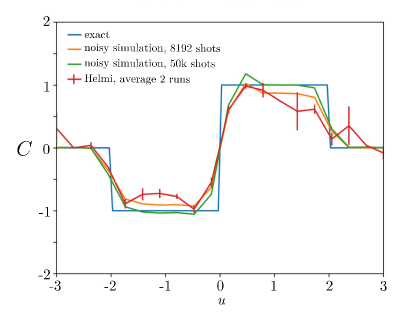
Figure 5: Chern number of the QWZ model. The Chern number is shown as a function of the on-site potential $u$. Results from Helmi are compared with exact results and simulations.

The Qi-Wu-Zhang (QWZ) model describes a two-dimensional topological insulator with a non-vanishing Chern number.Qi et al. (2006) The bulk Hamiltonian reads

$$\begin{split}H_{\text{QWZ}}(\bm{k})&=\sin(k_{x})\sigma_{x}+\sin(k_{y})\sigma_{y}\\ &+\left[u+\cos(k_{x})+\cos(k_{y})\right]\sigma_{z},\end{split}$$ (20)

where the on-site potential $u$ controls the topological phase of the system. Indeed, the energy spectrum splits into two bands with gap-closings at $u=2,0,-2$. Between the gap-closings, one finds non-trivial topological phases with ${C}=-1$ for $-2<u<0$ and ${C}=1$ for $0<u<2$, and ${C}=0$ otherwise.J. Asbóth and Pályi (2016)

In Fig. 3, we show the hybrid Wannier center of the QWZ model for different on-site potentials together with the Chern numbers that we extract. Figure 3(a) shows the exact results that we obtain using the Wilson-loop algorithm in Eq. (8). In Figs. 3(b,c), we show results obtained with our tensor-network simulations of the quantum circuit in Fig. 2(a) with a 10-qubit quantum phase estimation algorithm. We show the probability density of the hybrid Wannier center $P(X_{W})$ obtained from the quantum phase estimation algorithm, using different bond dimensions in the two panels. In both cases, we find good agreement with the exact results in Figs. 3(a), and the Chern number can accurately be extracted from the winding of the Berry phase across the Brillouin zone. We find that the results do not depend strongly on the bond dimension, indicating that the algorithm may not be very susceptible to the loss of entanglement.

In Fig. 4, we show calculations of the Berry flux using the quantum circuit in Fig. 2(b). For this circuit, quantum calculations are performed using Helmi. For the sake of comparison, we also show exact results from the Wilson-loop algorithm as well as simulations of Helmi using the FakeAdonis() backend. To calculate the Berry flux, we discretize the Brillouin zone into a grid of $15\times 15$ plaquettes. Employing two evolution steps per link, meaning an adiabatic transformation by $2\pi/30$ degrees per time-evolution step, we obtain a circuit depth of 6 elementary single-site and 2 two-site gates per plaquette at the transpilation level 3. The results are then read out with $8192$ shots. Figure 4 shows the Berry flux across the extended Brillouin zone, with the first Brillouin zone, $[-\pi,\pi]\crossproduct[-\pi,\pi]$, highlighted by the dashed squares. Exact results are shown in the left column, while noisy simulations of the quantum circuit are presented in the middle column. In the right column, we show the results obtained experimentally with the Helmi quantum computer. Each row corresponds to different values of the on-site potential, which determines the topological phase of the system. Generally, we observe a good agreement between the calculations based on Helmi and both the exact results and those based on noisy simulations of Helmi. Importantly, from these calculations, we can extract the corresponding Chern numbers.

Figure 5 shows the Chern number obtained by integrating the Berry fluxes in Fig. 4 over the unit cell. The results from Helmi are averaged over two runs, and the error bars indicate the difference between the largest and the smallest values. We also show the exact results as well as results obtained from noisy simulations of Helmi. The results from Helmi clearly allow us to distinguish the different topological phases of the system. However, the results from Helmi and the noisy simulations are often smaller than the exact Chern number, which is an integer. However, we see that this issue can be resolved by increasing the number of measurements for the noisy simulations. This observation is consistent with the fact that the Hadamard test is very sensitive to the measurement precision, since the measurement frequencies enter into an inverse trigonometric function.

To summarize, we find that both circuits in Fig. 2 make it possible to determine the Chern numbers of the QWZ model with error margins that generally are small.

III.2 Haldane model

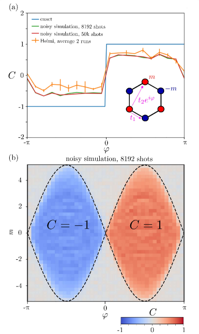
Figure 6: Topological classification of the Haldane model. (a) Chern number as a function of the phase with zero mass. Results obtained from Helmi are compared with the exact results and noisy simulations. (b) Full topological phase diagram obtained by noisy simulations of Helmi. The dashed lines indicate the exact phase boundaries given by Eq. (23).

As our second application, we consider the topological classification of the Haldane model. The Haldane model describes a two-dimensional Chern insulator on a honeycomb lattice. As illustrated in the inset of Fig. 6(a), the model involves nearest-neighbor and next-nearest-neighbor hopping with amplitudes $t_{1}$ and $t_{2}e^{i\varphi}$, where $\varphi$ is a tunable phase. The bulk Hamiltonian reads

$$H(\bm{k})=\bm{d}(\bm{k})\cdot\bm{\sigma},$$ (21)

where the vector $\bm{\sigma}$ contains the Pauli matrices. The three components of the vector $\bm{d}(\bm{k})$ are

$$\begin{split}d^{x}(\bm{k})=&t_{1}[\cos(\bm{k}\cdot\bm{a}_{1})+\cos(\bm{k}\cdot\bm{a}_{2})+1],\\ d^{y}(\bm{k})=&t_{1}[\sin(\bm{k}\cdot\bm{a}_{1})+\sin(\bm{k}\cdot\bm{a}_{2})],\\ d^{z}(\bm{k})=&m+2t_{2}\sin(\varphi)[\sin(\bm{k}\cdot\bm{a}_{1})-\sin(\bm{k}\cdot\bm{a}_{2})\\ &-\sin(\bm{k}\cdot(\bm{a}_{1}-\bm{a}_{2}))],\end{split}$$ (22)

where the last term in $d^{z}(\bm{k})$ breaks time-reversal symmetry. The unit cell is spanned by the vectors $\bm{a}_{1}=(\sqrt{3}/2,1/2)\quad\mathrm{and}\quad\bm{a}_{2}=(\sqrt{3}/2,-1/2)$, and the topological phase is controlled by the values of $m$ and $\varphi$. In the following, we focus on the case $t_{1}=t_{2}=1$, where the system exhibits two topologically nontrivial phases. Specifically, the expected Chern numbers are

$$\begin{split}{C}=-1,&\quad|m|<3\sqrt{3}|\sin(\varphi)|,\,\,-\pi<\varphi<0,\\ {C}=+1,&\quad|m|<3\sqrt{3}|\sin(\varphi)|,\,\,\phantom{-}0<\varphi<\pi,\\ {C}=\phantom{+}0,&\quad\text{otherwise (for }m\neq 0).\end{split}$$ (23)

In Fig. 6, we show the topological phase diagram of the Haldane model computed with the quantum circuit in Fig. 2(b) using a $15\times 15$ grid in the Brillouin zone. In Fig. 6(a) we show the Chern numbers obtained with Helmi as a function of the tunable phase and a zero mass. For the sake of comparison, we also show the exact results as well as noisy simulations. Also in this case, we observe a good qualitative agreement between the quantum computations and the exact results. Still, the quantum computations yield results that are somewhat smaller than the expected integer values of the Chern number. Nevertheless, by rounding off to the closest integer, the results clearly allow us to distinguish between the topologically trivial and non-trivial phases. Finally, in Fig. 6(b), we show the complete topological phase diagram of the Haldane model obtained with a noisy simulation. Here, we also observe a good agreement with the exact phase boundaries given by Eq. (23), shown with dashed lines.

IV Conclusions

We have presented quantum computations of Chern numbers for two-dimensional quantum matter. To this end, we have described two quantum circuits that are based on the adiabatic evolution of a quantum state in momentum space. The first circuit uses the quantum phase estimation algorithm to determine the Berry phase. We can thereby extract the winding of the corresponding Wannier center across the unit cell, which directly yields the Chern number. This circuit requires many qubits to reach a high precision, and we have therefore simulated it using our tensor-network simulator of quantum circuits. The second circuit, by contrast, relies on calculations of the Berry flux through a grid of plaquettes in the Brillouin zone. The Berry flux associated with each plaquette is small enough that it can be read out using a Hadamard test. For this reason, the number of qubits in this circuit is small enough that it can be implemented on the quantum computer Helmi. As specific applications, we have considered the topological classification of the Qi-Wu-Zhang (QWZ) model and the Haldane model. For the QWZ model, we made use of both quantum circuits and found that the first circuit, based on the quantum phase estimation algorithm, can be implemented with a modest level of entanglement. With the second circuit, we found that the topological phases can be correctly identified using Helmi. The same conclusion was reached when calculating the topological phase diagram of the Haldane model using Helmi. For the second circuit, we found that it works well with a small number of evolution steps per link. The quantum circuit is therefore rather shallow and requires fewer qubits than the first circuit. Our approach can be generalized to other topological invariants and may be applied to other systems such as $Z_{2}$ topological insulators or topological semimetals. Ultimately, the circuits may be implemented for interacting many-body Hamiltonians, where the many-body ground state is obtained via a variational eigensolver. As such, they provide a way forward towards classifying strongly interacting quantum matter using quantum computers.

V Acknowledgments

We acknowledge the financial support from InstituteQ, the Jane and Aatos Erkko Foundation, the Aalto Science Institute, the Research Council of Finland through the Finnish Centre of Excellence in Quantum Technology (352925) and projects No. 331342 and 358088, and the Japan Society for the Promotion of Science through an Invitational Fellowship for Research in Japan. We acknowledge the computational resources provided by the Aalto Science-IT project, CSC and the FiQCI quantum computing infrastructure.

References

- Qi and Zhang (2011) X.-L. Qi and S.-C. Zhang, “Topological insulators and superconductors,” Rev. Mod. Phys. 83, 1057 (2011).
- Hasan and Kane (2010) M. Z. Hasan and C. L. Kane, “Colloquium: Topological insulators,” Rev. Mod. Phys. 82, 3045 (2010).
- Moessner and Moore (2021) R. Moessner and J. E. Moore, Topological Phases of Matter (Cambridge University Press, 2021).
- J. Asbóth and Pályi (2016) L. Oroszlány J. Asbóth and A. Pályi, A Short Course on Topological Insulators (Springer, 2016).
- Xiao et al. (2010) D. Xiao, M.-C. Chang, and Q. Niu, “Berry phase effects on electronic properties,” Rev. Mod. Phys. 82, 1959 (2010).
- Ren et al. (2016) Y. Ren, Z. Qiao, and Q. Niu, “Topological phases in two-dimensional materials: a review,” Rep. Prog. Phys. 79, 066501 (2016).
- Chang et al. (2023) C.-Z. Chang, C.-X. Liu, and A. H. MacDonald, “Colloquium: Quantum anomalous Hall effect,” Rev. Mod. Phys. 95, 011002 (2023).
- Maciejko et al. (2011) J. Maciejko, T. L. Hughes, and S.-C. Zhang, “The Quantum Spin Hall Effect,” Annu. Rev. Condens. Matter Phys. 2, 31 (2011).
- Alicea (2012) J. Alicea, “New directions in the pursuit of Majorana fermions in solid state systems,” Rep. Prog. Phys 75, 076501 (2012).
- Berry (1984) M. V. Berry, “Quantal phase factors accompanying adiabatic changes,” Proc. R. Soc. Lond. A 392, 45 (1984).
- Zak (1989) J. Zak, “Berry’s phase for energy bands in solids,” Phys. Rev. Lett. 62, 2747 (1989).
- Haldane (1988) F. D. M. Haldane, “Model for a Quantum Hall Effect without Landau Levels: Condensed-Matter Realization of the ”Parity Anomaly”,” Phys. Rev. Lett. 61, 2015 (1988).
- Kane and Mele (2005) C. L. Kane and E. J. Mele, “Quantum Spin Hall Effect in Graphene,” Phys. Rev. Lett. 95, 226801 (2005).
- Kitaev (2001) A. Yu. Kitaev, “Unpaired Majorana fermions in quantum wires,” Phys.-Usp. 44, 131 (2001).
- Alicea et al. (2011) J. Alicea, Y. Oreg, G. Refael, F. von Oppen, and M. P. A. Fisher, “Non-Abelian statistics and topological quantum information processing in 1D wire networks,” Nat. Phys. 7, 412 (2011).
- Nayak et al. (2008) C. Nayak, S. H. Simon, A. Stern, M. Freedman, and S. Das Sarma, “Non-Abelian anyons and topological quantum computation,” Rev. Mod. Phys. 80, 1083 (2008).
- Lahtinen and Pachos (2017) V. Lahtinen and J. Pachos, “A Short Introduction to Topological Quantum Computation,” SciPost Phys. 3, 21 (2017).
- T. Fukui and Suzuki (2005) Y. Hatsugai T. Fukui and H. Suzuki, “Chern Numbers in Discretized Brillouin Zone: Efficient Method of Computing (Spin) Hall Conductances,” J. Phys. Soc. Jpn. 74, 1674 (2005).
- K. Kudo and Hatsugai (2019) T. Kariyado K. Kudo, H. Watanabe and Y. Hatsugai, “Many-Body Chern Number without Integration,” Phys. Rev. Lett. 122, 146601 (2019).
- Ayral et al. (2023) T. Ayral, P. Besserve, D. Lacroix, and E. A. Ruiz Guzman, “Quantum computing with and for many-body physics,” (2023), arXiv:2303.04850 [quant-ph] .
- B. Murta and Fernández-Rossier (2020) G. Catarina B. Murta and J. Fernández-Rossier, “Berry phase estimation in gate-based adiabatic quantum simulation,” Phys. Rev. A 101, 020302 (2020).
- Semeghini et al. (2021) G. Semeghini, H. Levine, A. Keesling, S. Ebadi, T. T. Wang, D. Bluvstein, R. Verresen, H. Pichler, M. Kalinowski, R. Samajdar, A. Omran, S. Sachdev, A. Vishwanath, M. Greiner, V. Vuletić, and M. D. Lukin, “Probing topological spin liquids on a programmable quantum simulator,” Science 374, 1242 (2021).
- X. Xiao and Kemper (2021) J. K. Freericks X. Xiao and A. F. Kemper, “Determining quantum phase diagrams of topological Kitaev-inspired models on NISQ quantum hardware,” Quantum 5, 553 (2021).
- X. Xiao and Kemper (2023) J. K. Freericks X. Xiao and A. F. Kemper, “Robust measurement of wave function topology on NISQ quantum computers,” Quantum 7, 987 (2023).
- Sugimoto (2023) T. Sugimoto, “Quantum-circuit algorithms for many-body topological invariant and Majorana zero mode,” (2023), arXiv:2304.13408 .
- Mei et al. (2020) F. Mei, Q. Guo, Y.-F. Yu, L. Xiao, S.-L. Zhu, and S. Jia, “Digital Simulation of Topological Matter on Programmable Quantum Processors,” Phys. Rev. Lett. 125, 160503 (2020).
- Smith et al. (2022) A. Smith, B. Jobst, A. G. Green, and F. Pollmann, “Crossing a topological phase transition with a quantum computer,” Phys. Rev. Res. 4, L022020 (2022).
- Azses et al. (2020) D. Azses, R. Haenel, Y. Naveh, R. Raussendorf, E. Sela, and E. G. Dalla Torre, “Identification of Symmetry-Protected Topological States on Noisy Quantum Computers,” Phys. Rev. Lett. 125, 120502 (2020).
- K. Choo and Neupert (2018) N. Regnault K. Choo, C. W. von Keyserlingk and T. Neupert, “Measurement of the Entanglement Spectrum of a Symmetry-Protected Topological State Using the IBM Quantum Computer,” Phys. Rev. Lett. 121, 086808 (2018).
- Roushan et al. (2014) P. Roushan, C. Neill, Yu Chen, M. Kolodrubetz, C. Quintana, N. Leung, M. Fang, R. Barends, B. Campbell, Z. Chen, B. Chiaro, A. Dunsworth, E. Jeffrey, J. Kelly, A. Megrant, J. Mutus, P. J. J. O’Malley, D. Sank, A. Vainsencher, J. Wenner, T. White, A. Polkovnikov, A. N. Cleland, and J. M. Martinis, “Observation of topological transitions in interacting quantum circuits,” Nature 515, 241 (2014).
- Flurin et al. (2017) E. Flurin, V. V. Ramasesh, S. Hacohen-Gourgy, L. S. Martin, N. Y. Yao, and I. Siddiqi, “Observing Topological Invariants Using Quantum Walks in Superconducting Circuits,” Phys. Rev. X 7, 031023 (2017).
- Xu et al. (2018) X.-Y. Xu, Q.-Q. Wang, W.-W. Pan, K. Sun, J.-S. Xu, G. Chen, J.-S. Tang, M. Gong, Y.-J. Han, C.-F. Li, and G.-C. Guo, “Measuring the Winding Number in a Large-Scale Chiral Quantum Walk,” Phys. Rev. Lett. 120, 260501 (2018).
- Zhan et al. (2017) X. Zhan, L. Xiao, Z. Bian, K. Wang, X. Qiu, B. C. Sanders, W. Yi, and P. Xue, “Detecting Topological Invariants in Nonunitary Discrete-Time Quantum Walks,” Phys. Rev. Lett. 119, 130501 (2017).
- R.-Y. Sun and Yunoki (2023) T. Shirakawa R.-Y. Sun and S. Yunoki, “Efficient variational quantum circuit structure for correlated topological phases,” (2023), arXiv:2303.17187 .
- Hel (2024a) “Technical details about helmi,” (2024a), accessed: 2024-03-06.
- Luongo (2023) A. Luongo, “Quantum algorithms for data analysis,” (2023), accessed: 2023-10-12.
- Kitaev (1995) A. Yu. Kitaev, “Quantum measurements and the Abelian Stabilizer Problem,” (1995), arXiv:quant-ph/9511026 .
- Nielsen and Chuang (2010) M. A. Nielsen and I. L. Chuang, Quantum Computation and Quantum Information: 10th Anniversary Edition (Cambridge University Press, 2010).
- Marzari and Vanderbilt (1997) N. Marzari and D. Vanderbilt, “Maximally localized generalized Wannier functions for composite energy bands,” Phys. Rev. B 56, 12847 (1997).
- Coh and Vanderbilt (2009) S. Coh and D. Vanderbilt, “Electric Polarization in a Chern Insulator,” Phys. Rev. Lett. 102, 107603 (2009).
- Wu et al. (2018) Q. Wu, S. Zhang, H.-F. Song, M. Troyer, and A. A. Soluyanov, “Wanniertools: An open-source software package for novel topological materials,” Comput. Phys. Commun. 224, 405 (2018).
- Yu et al. (2011) R. Yu, X. L. Qi, A. Bernevig, Z. Fang, and X. Dai, “Equivalent expression of topological invariant for band insulators using the non-Abelian Berry connection,” Phys. Rev. B 84, 075119 (2011).
- Gresch et al. (2017) D. Gresch, G. Autès, O. V. Yazyev, M. Troyer, D. Vanderbilt, B. A. Bernevig, and A. A. Soluyanov, “Z2Pack: Numerical implementation of hybrid Wannier centers for identifying topological materials,” Phys. Rev. B 95, 075146 (2017).
- Soluyanov and Vanderbilt (2011) A. A. Soluyanov and D. Vanderbilt, “Computing topological invariants without inversion symmetry,” Phys. Rev. B 83, 235401 (2011).
- Tilly et al. (2022) J. Tilly, H. Chen, S. Cao, D. Picozzi, K. Setia, Y. Li, E. Grant, L. Wossnig, I. Rungger, H. H. Booth, and J. Tennyson, “The variational quantum eigensolver: A review of methods and best practices,” Phys. Rep. 986, 1 (2022).
- Note (1) All of these values are subject to daily fluctuations and are averaged over all five qubits Hel (2024b).
- Schollwöck (2011) U. Schollwöck, “The density-matrix renormalization group in the age of matrix product states,” Ann. Phys. 326, 96 (2011).
- Niedermeier et al. (2023) M. Niedermeier, J. L. Lado, and C. Flindt, “Tensor-Network Simulations of Noisy Quantum Computers,” (2023), arXiv:2304.01751 .
- Zhou et al. (2020) Y. Zhou, E. M. Stoudenmire, and X. Waintal, “What Limits the Simulation of Quantum Computers?” Phys. Rev. X 10, 041038 (2020).
- Stoudenmire and Waintal (2023) E. M. Stoudenmire and X. Waintal, “Grover’s Algorithm Offers No Quantum Advantage,” (2023), arXiv:2303.11317 .
- Ayral et al. (2023) T. Ayral, T. Louvet, Y. Zhou, C. Lambert, E. M. Stoudenmire, and X. Waintal, “Density-Matrix Renormalization Group Algorithm for Simulating Quantum Circuits with a Finite Fidelity,” PRX Quantum 4, 020304 (2023).
- Wang et al. (2017) D. S. Wang, C. D. Hill, and L. C. L. Hollenberg, “Simulations of Shor’s algorithm using matrix product states,” Quant. Inf. Process. 16 (2017).
- Dang et al. (2019) A. Dang, C. D. Hill, and L. C. L. Hollenberg, “Optimising Matrix Product State Simulations of Shor’s Algorithm,” Quantum 3, 116 (2019).
- Woolfe et al. (2017) K. J. Woolfe, C. D. Hill, and L. C. L. Hollenberg, “Scaling and efficient classical simulation of the quantum Fourier transform,” Quant. Inf. Comput. 17, 1 (2017).
- Fishman et al. (2022) M. Fishman, S. R. White, and E. M. Stoudenmire, “The ITensor Software Library for Tensor Network Calculations,” SciPost Phys. Codebases , 4 (2022).
- Niedermeier (2024) M. Niedermeier, “Quantunity,” (2024), accessed: 2023-03-26.
- Qi et al. (2006) X.-L. Qi, Y.-S. Wu, and S.-C. Zhang, “Topological quantization of the spin Hall effect in two-dimensional paramagnetic semiconductors,” Phys. Rev. B 74, 085308 (2006).
- Note (2) The probability density is computed as where are the Berry phases obtained from the quantum phase estimation algorithm, and the small parameter broadens the peaks.
- Hel (2024b) “Helmi commercial documentation,” (2024b), accessed: 2024-03-19.