Integrated empirical measures and generalizations of classical goodness-of-fit statistics

Abstract

Based on $m$-fold integrated empirical measures, we study three new classes of goodness-of-fits tests, generalizing Anderson-Darling, Cramér-von Mises, and Watson statistics, respectively, and examine the corresponding limiting stochastic processes. The limiting null distributions of the statistics all lead to explicitly solvable cases with closed-form expressions for the corresponding Karhunen-Loève expansions and covariance kernels. In particular, the eigenvalues are shown to be $\frac{1}{k(k+1)\cdots(k+2m-1)}$ for the generalized Anderson-Darling, $\frac{1}{(\pi k)^{2m}}$ for the generalized Cramér-von Mises, and $\frac{1}{2\pi\lceil k/2\rceil^{2m}}$ for the generalized Watson statistics, respectively. The infinite products of the resulting moment generating functions are further simplified to finite ones so as to facilitate efficient numerical calculations. These statistics are capable of detecting different features of the distributions and thus provide a useful toolbox for goodness-of-fit testing.

,

1 Introduction

1.1 Scope and summary

For more than seven decades, empirical processes have been one of the main tools used in understanding the behaviors of many goodness-of-fit tests defined via empirical distributions. We explore in this paper the usage of the less addressed iterated empirical measures in generalizing the classical goodness-of-fit tests, focusing on the rarely available explicitly solvable cases.

Three classical goodness-of-fit statistics.

Assume that $\{X_{1},\ldots,X_{N}\}$ is an independent and identically distributed (i.i.d.) sequence of random variables with a common cumulative distribution function $F$. In the one sample setting, the goodness-of-fit test is formulated as a test for the hypotheses

$$H_{0}:F=F_{0}\ \ \mbox{against}\ \ H_{1}:F\neq F_{0}.$$

When $F_{0}$ is a continuous distribution, we may assume, without loss of generality, that $F_{0}(x)=x$, the uniform distribution on $[0,1]$. Since the empirical distribution function $F_{N}(x):=\frac{1}{N}\sum_{1\leqslant i\leqslant N}\mathds{1}_{\{X_{i}\leqslant x\}}$ provides a natural estimator of $F(x)$ with $\mathds{1}_{\{\cdot\}}$ the indicator function, a good means of measuring the discrepancy between $F$ and $F_{0}$ is to compute the integrated squared difference between $F_{N}$ and $F_{0}$ with a suitable weight function. Among the large number of such statistics, three simple, effective and widely used ones are: the Cramér-von Mises statistic

$$\omega_{N}=N\int_{0}^{1}(F_{N}(x)-x)^{2}\,\mathrm{d}x$$

(Cramér, 1928; von Mises, 1931; Smirnov, 1937), the Anderson-Darling statistic

$$A_{N}=N\int_{0}^{1}\frac{(F_{N}(x)-x)^{2}}{x(1-x)}\,\mathrm{d}x$$

(Anderson and Darling, 1952), and Watson’s ($U^{2}$-) statistic

$$U_{N}=N\int_{0}^{1}\biggl{(}F_{N}(x)-x-\int_{0}^{1}(F_{N}(t)-t)\,\mathrm{d}t\biggr{)}^{2}\,\mathrm{d}x$$

(Watson, 1961). For historical and technical reasons (some explained below), these are generally regarded as the de facto standards in the area of quadratic statistics based on empirical distribution functions. Briefly, the Anderson-Darling statistic has more power than the Cramér-von Mises statistic in the tail area of the distribution due specially to the choice of the variance-based weight function $\mathrm{Var}(F_{N}(x))=\frac{x(1-x)}{N}$ under the null hypothesis $H_{0}$. On the other hand, Watson’s statistic is designed for testing the uniformity of periodic data with period 1 so that $X_{i}+1\equiv X_{i}$.

In addition to integral-type goodness-of-fit statistics, the literature also abounds with other types such as the maximum-type statistics, one representative being the Kolmogorov-Smirnov statistic, defined as the maximum of the integrand of the Cramér-von Mises statistic:

$$D_{N}=\sqrt{N}\sup_{x\in[0,1]}|F_{N}(x)-x|.$$

Similarly, the maximum of the integrand of the Anderson-Darling statistic can be defined. In particular, the maximizer or the point maximizing the statistic of these maximum-type statistics indicates more precisely how discrepant the empirical distribution to the null distribution is. Such test statistics have a similar structure to estimating the change-point in regression analysis on the unit interval, where the maximizer is an estimate of the change-point. We will discuss briefly this viewpoint again later.

Explicit Karhunen-Loève expansions.

An important property possessed by the three classical statistics is their explicitly solvable eigenstructures in the corresponding limiting Gaussian processes of the signed square-root of the integrand. For example, the stochastic process arising from the Anderson-Darling statistic, defined as the limit of the map

$$x\mapsto\sqrt{N}\frac{F_{N}(x)-x}{\sqrt{x(1-x)}},$$

under the null hypothesis $H_{0}$, has the limiting Gaussian process ($B(x)$ being a Brownian bridge)

$$x\mapsto A(x):=\frac{B(x)}{\sqrt{x(1-x)}},$$

which has an explicit eigenfunction expansion referred to as the Karhunen-Loève (KL) expansion

$$A(x)=\sum_{k\geqslant 1}\frac{1}{\sqrt{\lambda_{k}}}\,f_{k}(x)\xi_{k};$$

here $\lambda_{k}^{-1}$ are the eigenvalues with $\lambda_{k}:=k(k+1)$, $f_{k}$ are eigenfunctions expressible in terms of the Legendre polynomials, and $\xi_{k}$ are i.i.d. random variables with the standard normal distribution $N(0,1)$; see Theorem 2.3 for a more precise formulation.

The corresponding eigenvalues for the other two classical statistics are given by $\lambda_{k}^{-1}$ with $\lambda_{k}=(\pi k)^{2}$ (Cramér-von Mises) and $\lambda_{k}=2\pi\bigl{\lceil}\frac{k}{2}\bigr{\rceil}^{2}$ (Watson), respectively, and the eigenfunctions are both expressible in terms of trigonometric functions. Such explicit expansions proved to be advantageous for most qualitative and numerical purposes, notably in computing the density or the tail probabilities of the limiting distribution (of the statistic); see the discussions after Theorem 2.4 and (45). Also the feature of a few leading eigenfunctions $f_{1},f_{2},\ldots$ can be used to determine the statistical power of the goodness-of-fit under local alternatives (Durbin and Knott (1972); see also Sec. 2.5). In the words of Deheuvels and Martynov (2008):

Unfortunately, for most Gaussian processes of interest with respect to statistics, the values of the $\lambda_{k}$’s are unknown, even though their existence remains guaranteed …The practical application of this theory to statistics is therefore limited to a small number of particular cases. …

In addition to the three statistics, some other fortunate examples of tests whose KL expansions are explicitly identified are collected in Sec. 1.2.

On the other hand, the “small ball asymptotics” in probability represents another context that is closely connected to the study of goodness-of-fit statistics of integral-type. As in the context here, explicit eigenstructures prove useful and informative; see e.g., Chen and Li (2003), Gao et al. (2003), Nikitin and Pusev (2013), and the references therein.

In general, the goodness-of-fit statistics of integral-type are constructed as positive-definite quadratic forms of the empirical measure $\,\mathrm{d}F_{N}(x)$. Thus weighted infinite sums of chi-square random variables of the form

$$\sum_{k\geqslant 1}\frac{\xi_{k}^{2}}{\lambda_{k}},\quad\xi_{k}\sim N(0,1)\;\mbox{i.i.d.}$$ (1)

appear naturally as the limit laws. However, to determine the eigenstructure, we are led to the boundary-value problem involving an integral equation whose covariance kernel is often not exactly solvable. For example, Lockhart and Stephens (1998) mentioned that the limiting distribution of Shapiro and Wilk (1965)’s statistic was of the form (1), but its weights remained unknown in general.

On the other hand, it is well-known that the decay order of the eigenvalues is determined by the smoothness of the covariance kernel, so that even no closed-form expressions are available, one can often deduce the required properties from smoothness of the covariance kernel; see Chang and Ha (1999); Cochran and Lukas (1988) for more information.

Explicit formulae for the moment generating functions of the limiting null distributions.

From (1), one has the following explicit form for the moment generating function (MGF)

$$\mathbb{E}\exp\biggl{(}s\sum_{k\geqslant 1}\frac{\xi_{k}^{2}}{\lambda_{k}}\biggr{)}=\prod_{k\geqslant 1}\frac{1}{\sqrt{1-\frac{2s}{\lambda_{k}}}},$$ (2)

and for the three classical statistics, the corresponding MGFs can be further simplified as follows.

Anderson-Darling		Cramér-von Mises		Watson
$\displaystyle\sqrt{\frac{-2\pi s}{\cos\frac{\pi}{2}\sqrt{1+8s}}}$		$\displaystyle\sqrt{\frac{\sqrt{2s}}{\sin\sqrt{2s}}}$		$\displaystyle\frac{\sqrt{\frac{s}{2}}}{\sin\sqrt{\frac{s}{2}}}$

These representations in lieu of the infinite products (2) are more useful for computational and analytic purposes; see Sec. 2.7.

Contributions of this paper.

In this paper, we propose three classes of goodness-of-fit statistics based on the $m$-fold integral of the empirical measure

$$\mathop{\int\cdots\int}_{0<x_{1}<\cdots<x_{m}<x}\,\mathrm{d}F_{N}(x_{1})\,\mathrm{d}x_{1}\cdots\,\mathrm{d}x_{m}=\int_{0}^{x}\frac{(x-t)^{m-1}}{(m-1)!}\,\mathrm{d}F_{N}(t)\qquad(m\geqslant 1),$$

where $F_{N}(x)=\int_{0<x_{1}<x}\,\mathrm{d}F_{N}(x_{1})$, as generalizations of Anderson-Darling, Cramér-von Mises, and Watson statistics, so that they inherit the advantages (such as explicit KL expansions and explicit MGFs for the limit laws) of the original three statistics. We provide a systematic approach based on the use of “template functions” to generalize the classical statistics, and examine their limiting properties. Some properties of these generalized statistics are summarized in Table 1.1.

Table 1.1: Generalizations of the three classical statistics based on $m$-fold integrated empirical measure. Here $\eta_{j}$ denote the zeros of a polynomial equation; see (43).

Proposed test	Generalized Anderson- Darling	Generalized Cramér- von Mises	Generalized Watson
Eigenvalue $\lambda_{k}^{-1},k\geqslant 1$	$\frac{1}{k(k+1)\cdots(k+2m-1)}$	$\frac{1}{(\pi k)^{2m}}$	$\frac{1}{(2\pi\lceil k/2\rceil)^{2m}}$
Eigenfunction	associated Legendre	trigonometric function	trigonometric function
Covariance kernel	incomplete beta	Bernoulli polynomial	Bernoulli polynomial
MGF of the limit law	$\sqrt{\prod\limits_{j=0}^{m-1}\frac{-2\pi s}{(2j)!(2j+1)!\cos\bigl{(}{\pi\eta_{j}^{\frac{1}{2}}}\bigr{)}}}$	$\sqrt{\frac{e^{\frac{m-1}{2}\pi i}\sqrt{2s}}{\prod\limits_{j=0}^{m-1}\sin\bigl{(}(2s)^{\frac{1}{2m}}e^{\frac{j\pi i}{m}}\bigr{)}}}$	$\frac{2^{-m}e^{\frac{m-1}{2}\pi i}\sqrt{2s}}{\prod\limits_{j=0}^{m-1}\sin\bigl{(}\frac{1}{2}(2s)^{\frac{1}{2m}}e^{\frac{j\pi i}{m}}\bigr{)}}$

For example, the moment generating functions of the limiting distributions of the generalized Anderson-Darling statistic for $m=2$ has the following closed-form expression

$$\prod_{k\geqslant 1}\frac{1}{\sqrt{1-\frac{2s}{k(k+1)(k+2)(k+3)}}}=\frac{\pi s}{\sqrt{3\cos\left(\frac{\pi}{2}\sqrt{5-4\sqrt{1+2s}}\right)\cos\left(\frac{\pi}{2}\sqrt{5+4\sqrt{1+2s}}\right)}}$$

which is (Eq. (46) in Sec. 2.7). The explicit form for $m=3$ is also given in (47).

Some integrated empirical measures or Gaussian processes in the literature.

Goodness-of-fit tests based on the one-time integrated empirical measures was proposed by Henze and Nikitin (2000) in a way different from this paper. They obtained the asymptotic distribution in terms of one-time integrated Brownian bridge and the corresponding eigenvalues $\lambda_{k}$ are shown to be connected to the solutions of the equation $\tan\lambda^{\frac{1}{4}}+\tanh\lambda^{\frac{1}{4}}=0$, the corresponding eigenfunctions being expressible in terms of trigonometric and hyperbolic functions. Similarly, Watson-type tests and two-sample tests based on the integrated empirical measures were studied in Henze and Nikitin (2002) and in Henze and Nikitin (2003), respectively. Recently Durio and Nikitin (2016) pointed out that some integrated goodness-of fit tests have good statistical power for skew alternative.

In connection with ball probabilities of stochastic processes, Gao et al. (2003) showed that the eigenvalues $\lambda_{k}$ associated with the squared integral of the one-time integrated Brownian motion are expressible in terms of the real zeros of the equation $\cosh\lambda^{\frac{1}{4}}+\sec\lambda^{\frac{1}{4}}=0$, and provided the moment generating function explicitly. In the case of multi-fold integrated Brownian motion, Tanaka (2008) illustrated the use of Fredholm determinant approach to deriving the KL expansion; see also Chap. 5 of Tanaka (2017).

Integrated processes and change-point analysis in regression

The detection of change-points is of fundamental interest in statistical data analyses. In a typical setting, the change-point analysis aims at detecting the change of the mean in time series data. For that purpose, the difference in the sample mean before and after a candidate of change-point is used as a scan statistic. However, the changes to be detected are not necessarily limited to the mean parameter. MacNeill (1978a, b) discussed the change of parameters when a polynomial regression is used to fit the time series data. He proposed test statistics based on the accumulated (integrated) residuals, and derived their asymptotic distributions in terms of functionals of a Brownian motion. The same idea was also examined in Hirotsu (1986, 2017). In the analysis of ordered categorical data, he proposed to classify rows and/or columns by detecting change-points among the rows/columns. He pointed out that sometimes the change is observed as the change of convexity/concavity of response curves, and the accumulated statistic is useful for such detection purposes. The integrated empirical processes proposed here are regarded as generalizations of their statistics.

Organization of the paper.

In Sec. 1.2, we give a brief historical account relating to the statistics we propose. In particular, some goodness-of-fit statistics of integral-type with explicit eigenstructure are gathered there. In Sec. 2, a class of generalized Anderson-Darling statistics is proposed. From the limiting null distribution of the integrand of the statistics, we define and study the (generalized) Anderson-Darling process, with its KL expansion and the covariance kernel given in explicit forms. Sections 3 and 4 then deal with the generalized Watson and Cramér-von Mises statistics and the associated processes, and discuss the corresponding KL expansions, the covariance kernels, and eigenfunction expansions. We also simplify the infinite-product representations in all cases of the moment generating functions of the limiting distributions, and compare the statistical power of the statistics by Monte Carlo simulations.

1.2 A brief review of related literature

As the literature on integral types of goodness-of-fit tests is vast, we content ourselves with a brief summary of integral tests of the form

$$N\int_{0}^{1}(F_{N}(x)-x)^{2}\varphi(x)\,\mathrm{d}x,$$ (3)

(with different $\varphi$) whose eigen-structures are explicitly known. For more information on the subject, see for example the books Durbin (1973), Shorack and Wellner (1986), Nikitin (1995), and Martynov (2015), D’Agostino (2017), and the survey papers González-Manteiga and Crujeiras (2013) and Broniatowski and Stummer (2022).

Test statistics with explicit KL expansions.

We list some examples connected to goodness-of-fit and related tests whose eigenstructures are explicitly known; this list is not intended to be exhaustive or comprehensive, but for easier comparison with our results.

As already stated, MacNeill (1978b, a) proposed test statistics in terms of an integrated empirical measure to detect the change points in polynomial regressions. The eigenstructure of the limiting Gaussian process is explicitly given; in particular, the eigenvalues are expressible in terms of the zeros of spherical Bessel functions, and the eigenfunctions in terms of associated Legendre polynomials.

Deheuvels (1981) proposed a statistic for testing independence in $m$-variate observations. An explicit KL expansion for the process defined as the limit of the integral test is derived. The eigenvalue has multiple indices $\lambda_{k_{1},\ldots,k_{m}}=\frac{2^{m/2}}{k_{1}\cdots k_{m}\pi^{m}}$ ($k_{j}\geqslant 1$) with the corresponding eigenfunctions given by $\prod_{1\leqslant j\leqslant m}\sin(k_{j}\pi u_{j})$. Deheuvels and Martynov (2003) defined the weighted Wiener process and Brownian bridge with weight function $\varphi(t)=t^{\beta}$ ($\beta>-1$), and obtained their Karhunen-Loève expansions in terms of the zeros of Bessel functions. A multivariate extension with weight function $\varphi(t)=\prod_{i}t_{i}^{\beta_{i}}$ was given in Deheuvels (2005). In testing independence for a bivariate survival function, Deheuvels and Martynov (2008) proved that under the null hypothesis, the proposed test statistic has an explicit Karhunen-Loève expansion with eigenvalues $\frac{1}{k(k+1)(k+2)(k+3)}$ ($k\geqslant 1$) and eigenfunctions in terms of the modified Jacobi polynomials. Note that this sequence of eigenvalues is the same as our generalized Anderson-Darling statistic when $m=2$; see Table 1.1.

Pycke (2003) studied an $m$-variate extension of the Anderson-Darling statistic. The eigenvalues now have the form $\lambda_{k}=\frac{m}{k(k+1)}$ ($k\geqslant 1$) and the corresponding eigenfunctions are expressible using the associated Legendre function.

Baringhaus and Henze (2008) proposed a class of goodness-of-fit statistics for exponentiality. The KL expansion appearing in the limit law has eigenvalues in terms of the zeros of the Bessel functions with Bessel eigenfunctions.

As mentioned in Introduction, eigenvalue problem for deriving KL expansion is closely related to the boundary-value problem. For example, Chang and Ha (2001) discussed a boundary-value problem with Bernstein and Euler polynomials as kernels, where the eigenvalues and eigenfunctions are given explicitly. Their results have a very close connection to our generalized Watson statistics; see Sec. 3. These results are summarized in Table 1.2.

Table 1.2: Tests with an explicit KL expansion

Test	Eigenvalue	Eigenfunction
$m$-variate test for independence (Deheuvels, 1981)	$\frac{2^{m/2}}{k_{1}\cdots k_{m}\pi^{m}}$	$\prod_{1\leqslant j\leqslant m}\sin(k_{j}\pi u_{j})$
Weighted Brownian motion/bridge (Deheuvels and Martynov, 2003)	zeros of Bessel (1st kind)	Bessel function
Independence of bivariate survival function (Deheuvels and Martynov, 2008)	$\frac{1}{k(k+1)(k+2)(k+3)}$	modified Jacobi polynomial
$m$-variate Anderson-Darling (Pycke, 2003)	$\frac{m}{k(k+1)}$	Legendre
Decomposition of Anderson-Darling (Rodríguez and Viollaz, 1999)	zeros of Bessel (1st kind)	Bessel function
Goodness-of-fit for exponentiality (Baringhaus and Henze, 2008)	zeros of Bessel (1st kind)	Bessel function
Bernoulli/Euler kernel boundary-value problem (Chang and Ha, 2001)		Bernoulli/Euler polynomial
Weighted, time-change Brownian Bridge (Pycke, 2021a, 2023)		Jacobi, Laguerre, Hermite, Krawtchouk polynomials

Weighted Cramér-von Mises statistics.

A natural extension of Anderson-Darling and Cramér-von Mises statistics is the quadratic statistics of the form (3), often referred to as weighted Cramér-von Mises statistics and extensively studied in the literature. Table 1.3 summarizes some variants studied in the literature. The eigenstructures of many of these statistics are not given explicitly.

Table 1.3: Some weighted Cramér-von Mises statistics

$\varphi(t)$	References
$1$	Cramér (1928), von Mises (1931)
$\frac{1}{t(1-t)}$	Anderson and Darling (1952)
$\Bigl{(}\log\frac{1}{t(1-t)}\Bigr{)}^{2}$	Groeneboom and Shorack (1981) (Shorack and Wellner, 1986, p. 227)
$\frac{1}{t}$, $\frac{1}{1-t}$	Sinclair, Spurr and Ahmad (1990), Scott (1999) Rodríguez and Viollaz (1999)
$\frac{1}{1-t^{2}}$, $\frac{1}{t(2-t)}$	Rodríguez and Viollaz (1995) Viollaz and Rodríguez (1996) Shi, Wang and Reid (2022)
$t^{\beta}$	Deheuvels and Martynov (2003) Deheuvels (2005)
$\frac{1}{\alpha^{2}t^{2-\frac{1}{\alpha}}\bigl{(}1-t^{\frac{1}{\alpha}}\bigr{)}}$	Mansuy (2005)
$\frac{1}{t^{2}}$, $\frac{1}{(1-t)^{2}}$	Luceño (2006) Chernobai, Rachev and Fabozzi (2015)
$\frac{1}{(1-t)^{\alpha}}$	Feuerverger (2016)
$\begin{array}[]{c}1,\ t^{2\beta},\ t^{2},\ t(1-t)\\ \bigl{(}t-\tfrac{1}{2}\bigr{)}^{2},\ \frac{1}{t(1-t)}\end{array}$	Medovikov (2016)
$\begin{array}[]{c}\mbox{\footnotesize$I^{-1}_{\nu_{1},\nu_{2}}(t)^{1-2\nu_{1}}I^{-1}_{\nu_{2},\nu_{1}}(1-t)^{1-2\nu_{2}}$}\\ \mbox{\footnotesize($I(\cdot)$: incomplete beta function)}\end{array}$	Pycke (2021b)
$\frac{1}{t^{3/2}}$, $\frac{1}{(1-t)^{3/2}}$	Ma, Kitani and Murakami (2022)
$\frac{1}{t^{2}(1-t)^{2}}$	Liu (2023)

2 The generalized Anderson-Darling statistics

In this section, we propose our new generalized Anderson-Darling statistics and examine their small-sample and large-sample properties in detail.

2.1 Legendre polynomials and the template functions

We construct first the template functions needed using Legendre polynomials.

Construction of the template functions.

The original Anderson-Darling statistic (4) can be written as

$$A_{N}=\int_{0}^{1}\frac{B_{N}(x)^{2}}{x(1-x)}\,\mathrm{d}x,\quad\mbox{where }\ B_{N}(x)=\sqrt{N}(F_{N}(x)-x).$$ (4)

Here we express $B_{N}(x)$ in terms of a template function $\tau_{1}(t;x)$:

$$B_{N}(x)=\sqrt{N}\int_{0}^{1}\tau_{1}(t;x)\,\mathrm{d}F_{N}(t),\quad\mbox{where }\ \tau_{1}(t;x):=\mathds{1}_{\{t\leqslant x\}}-x,$$ (5)

with $\mathds{1}_{\{t\leqslant x\}}=1$ if $t\leqslant x$, and $0$ otherwise.

The template function $t\mapsto\tau_{1}(t;x)$ is a piecewise constant function for $t\in[0,1]$ with a breakpoint at $x$, and orthogonal to any constant function, namely, $\int_{0}^{1}\tau_{1}(t;x)\,\mathrm{d}t=0$.

To extend this template function, we define $\tau_{2}(t;x)$ for $t\in[0,1]$ to be a function such that it is a continuous and piecewise linear function with a change point at $x$, and orthogonal to any linear function, namely, $\int_{0}^{1}\tau_{2}(t;x)(at+b)\,\mathrm{d}t=0$ for all $a,b\in\mathbb{R}$.

In general, we define the $m$-th template function $\tau_{m}(t;x)$ for $t\in[0,1]$ to be a $C^{m-2}$ and piecewise polynomial function of degree $m-1$ in $t$ with a turning point at $x$, and orthogonal to any polynomial function of degree $\leqslant m-1$, namely,

$$\int_{0}^{1}\tau_{m}(t;x)t^{j}\,\mathrm{d}t=0\qquad(j=0,1,\dots,m-1).$$ (6)

Definition 2.1 (Legendre polynomials $P_{k}(x)$).

The (shifted and normalized) Legendre polynomials are defined to be the polynomials of degree $k$ satisfying the orthogonality relations

$$\int_{0}^{1}P_{k}(t)P_{l}(t)\,\mathrm{d}t=\mathds{1}_{\{k=l\}}\qquad(k,l\geqslant 0).$$ (7)

Note that the $P_{k}(x)$ are nothing but the polynomials generated by the Gram-Schdmit orthogonalization procedure in the unit interval with the weight function $1$. They have the closed-form expression

$$P_{k}(x)=\sqrt{2k+1}\sum_{0\leqslant l\leqslant k}\scalebox{0.8}{$\dbinom{k}{l}$}\scalebox{0.8}{$\dbinom{k+l}{l}$}(-1)^{k+l}x^{l},$$ (8)

and satisfy the relation $P_{k}(1-x)=(-1)^{k}P_{k}(x)$. In particular, $P_{0}(x)=1$ and

$P_{1}(x)$	$P_{2}(x)$	$P_{3}(x)$
$\sqrt{3}(2x-1)$	$\sqrt{5}(6x^{2}-6x+1)$	$\sqrt{7}(20x^{3}-30x^{2}+12x-1)$

Also the leading coefficient is given by

$$[x^{k}]P_{k}(x)=\scalebox{0.8}{$\dbinom{2k}{k}$}\sqrt{2k+1},$$

where $[x^{k}]f(x)$ denotes the coefficient of $x^{k}$ in the Taylor expansion of $f(x)$.

For convenience, define the $m$-fold integral of the polynomial $P_{k}(x)$

$$P_{k}^{(-m)}(x)=\mathop{\int\cdots\int}_{0<t_{1}<\cdots<t_{m}<x}P_{k}(t_{1})\,\mathrm{d}t_{1}\cdots\,\mathrm{d}t_{m}=\int_{0}^{x}\frac{(x-t)^{m-1}}{(m-1)!}\,P_{k}(t)\,\mathrm{d}t.$$ (9)

The template functions we need are then given as follows.

Lemma 2.1.

For $m\geqslant 1$ and $x\in[0,1]$, let

$$\tau_{m}(t;x)=\frac{(x-t)^{m-1}}{(m-1)!}\,\mathds{1}_{\{t\leqslant x\}}-\sum_{0\leqslant k<m}P_{k}(t)P_{k}^{(-m)}(x).$$ (10)

Then $\tau_{m}(t;x)\in C^{m-2}$ for $t\in[0,1]$, satisfies (6) and is a piecewise polynomial function.

Proof.

Obviously, the template function $\tau_{m}$ is of $C^{m-2}$. Only (6) needs to be proved. For that purpose, it suffices to show that

$$\int_{0}^{x}\tau_{m}(t;x)P_{j}(t)\,\mathrm{d}u=0\qquad(0\leqslant j\leqslant m-1).$$ (11)

By definition,

$$\int_{0}^{1}\tau_{m}(t;x)P_{j}(t)\,\mathrm{d}t=P_{j}^{(-m)}(x)-\sum_{0\leqslant k<m}P_{k}^{(-m)}(x)\int_{0}^{1}P_{j}(t)P_{k}(t)\,\mathrm{d}t,$$

which, by the orthogonality relation (7), yields (11). ∎

Figure 2.1 depicts $\tau_{m}(\cdot;x)$ for $1\leqslant m\leqslant 4$.

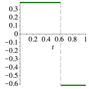
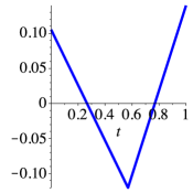
$\tau_{1}(t;x_{0})$	$\tau_{2}(t;x_{0})$
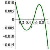
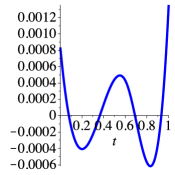
$\tau_{3}(t;x_{0})$	$\tau_{4}(t;x_{0})$

Figure 2.1: The template functions $\tau_{m}(t;x_{0})$ for the generalized Anderson-Darling statistics for $1\leqslant m\leqslant 4$; here $x_{0}=\frac{\sqrt{5}-1}{2}$, the reciprocal of the golden ratio.

Observe, by (8) and by a direct integration, that

$$P_{k}^{(-m)}(x)=\sqrt{2k+1}\sum_{0\leqslant j\leqslant k}\frac{(-1)^{k+j}(k+j)!}{j!(k-j)!(m+j)!}\,x^{m+j}.$$ (12)

Without signs and the normalizing factor $\sqrt{2k+1}$, $P_{k}(x)$ corresponds to sequence A063007 (and, up to a shift of index, A109983) in the Online Encyclopedia of Integer Sequences (OEIS, 2019), and $P_{k}^{(-1)}(x)$ to A088617; they all have direct combinatorial interpretations in terms of parameters on certain lattice paths. Note that $P_{k}^{(-1)}(x)$ also appeared in MacNeill (1978b) but in the form

$$\frac{(2k)!}{k!}\sum_{0\leqslant j\leqslant\lfloor k/2\rfloor}\frac{(-1)^{j}}{16^{j}j!^{2}(k-2j)!\binom{k-\frac{1}{2}}{j}}\int_{0}^{x}\bigl{(}{v-\tfrac{1}{2}}\bigr{)}^{k-2j}\,\mathrm{d}v,$$

which can be proved to be identical to (12) with $m=1$ and without the factor $\sqrt{2k+1}$.

2.2 The generalized Anderson-Darling statistic

With the template functions $\tau_{m}(t;x)$ at hand, we now define, similar to (5),

$$B^{[m]}_{N}(x) :=\sqrt{N}\int_{0}^{1}\tau_{m}(t;x)\,\mathrm{d}F_{N}(t)$$

$$=\sqrt{N}\Biggl{(}\mathop{\int\cdots\int}_{0<t_{1}<\cdots<t_{m}<x}\,\mathrm{d}F_{N}(t_{1})\,\mathrm{d}t_{2}\cdots\,\mathrm{d}t_{m}$$

$$\qquad\qquad-\sum_{0\leqslant k<m}P_{k}^{(-m)}(x)\int_{0}^{1}P_{k}(t)\,\mathrm{d}F_{N}(t)\Biggr{)}.$$ (13)

Note that $B^{[1]}_{N}(x)=B_{N}(x)$. Then, as in (4), we define the generalized Anderson-Darling (GAD) statistic as

$$A^{[m]}_{N}:=\int_{0}^{1}\frac{B^{[m]}_{N}(x)^{2}}{(x(1-x))^{m}}\,\mathrm{d}x,$$ (14)

which equals the original Anderson-Darling statistic when $m=1$ : $A^{[1]}_{N}=A_{N}$. However, unlike $A_{N}^{[1]}$, the variance of $B^{[m]}_{N}(x)$ in (13) with $x$ fixed is proportional to $(x(1-x))^{2m-1}$ (see Theorem 2.2), which is different from the denominator $(x(1-x))^{m}$ we used in (14) except for the case $m=1$. The motivation of choosing such a weight will become clear later.

On the other hand, it is less obvious whether the integral (14) exists because of the seemingly singular factors in the denominator at the end points. We now show that the GAD statistics $A^{[m]}_{N}$ can be expressed in terms of the samples $X_{i}$’s, $1\leqslant i\leqslant N$.

Lemma 2.2.

Assume $X_{i}\in(0,1)$ for $1\leqslant i\leqslant N$. Then the GAD statistics $A^{[m]}_{N}$ in (14) are well-defined for $m\geqslant 1$, and are invariant with respect to the changes $X_{i}\mapsto 1-X_{i}$ for all $i=1,\dots,N$.

Proof.

We first rewrite the template function $\tau_{m}(t;x)$. By the completeness of the Legendre polynomial system and the relation $P_{k}(1-x)=(-1)^{k}P_{k}(x)$,

$$\frac{(x-t)^{m-1}}{(m-1)!} =\sum_{0\leqslant k<m}P_{k}(t)\biggl{(}\int_{x}^{1}+\int_{0}^{x}\biggr{)}\frac{(x-u)^{m-1}}{(m-1)!}P_{k}(u)\,\mathrm{d}u$$

$$=(-1)^{m-1}\sum_{0\leqslant k<m}P_{k}(1-t)P_{k}^{(-m)}(1-x)+\sum_{0\leqslant k<m}P_{k}(t)P_{k}^{(-m)}(x).$$

Substituting this into (10), we obtain

$$\tau_{m}(t;x) =(-1)^{m-1}\sum_{0\leqslant k<m}P_{k}(1-t)P_{k}^{(-m)}(1-x)\mathds{1}_{\{t\leqslant x\}}$$

$$\qquad\qquad-\sum_{0\leqslant k<m}P_{k}(t)P_{k}^{(-m)}(x)\mathds{1}_{\{t>x\}}.$$ (15)

Now expanding the square in (14) as a double integral, giving

$$A^{[m]}_{N}=\int_{0}^{1}\int_{0}^{1}\biggl{(}\int_{0}^{1}\frac{\tau_{m}(t;x)\tau_{m}(u;x)}{(x(1-x))^{m}}\,\mathrm{d}x\biggr{)}\,\mathrm{d}F_{N}(t)\,\mathrm{d}F_{N}(u),$$

where the expression between the parentheses becomes, by (2.2),

$$\sum_{0\leqslant k,l<m}P_{k}(1-t)P_{l}(1-u)\int_{t\vee u}^{1}\frac{P_{k}^{(-m)}(1-x)P_{l}^{(-m)}(1-x)}{(x(1-x))^{m}}\,\mathrm{d}x$$ (16)

$$-(-1)^{m-1}\sum_{0\leqslant k,l<m}P_{k}(1-t\wedge u)P_{l}(t\vee u)\int_{t\wedge u}^{t\vee u}\frac{P_{k}^{(-m)}(1-x)P_{l}^{(-m)}(x)}{(x(1-x))^{m}}\,\mathrm{d}x$$

$$+\sum_{0\leqslant k,l<m}P_{k}(t)P_{l}(u)\int_{0}^{t\wedge u}\frac{P_{k}^{(-m)}(x)P_{l}^{(-m)}(x)}{(x(1-x))^{m}}\,\mathrm{d}x.$$

Since $P_{k}^{(-m)}(x)$ and $P_{k}^{(-m)}(1-x)$ contain factors of the forms $x^{m+j}$ and $(1-x)^{m+j}$ for $j\geqslant 0$ (see (12)), respectively, the three integrals in (16) are well-defined if $t\vee u<1$ and $t\wedge u>0$. On the other hand, (16) is invariant with respect to the change of variables $(t,u)\mapsto(1-t,1-u)$. ∎

With more calculations, it is possible to derive a more precise expression for $A_{N}^{[m]}$.

Lemma 2.3.

Let $a_{ij}=X_{i}\wedge X_{j}$ and $b_{ij}=1-X_{i}\vee X_{j}$. Then

$$A_{N}^{[m]}=-\text{\scalebox{0.9}{$\frac{1}{N}$}}\sum_{1\leqslant i,j\leqslant N}R_{m}(a_{ij},b_{ij})(\log a_{ij}+\log b_{ij})+\text{\scalebox{0.9}{$\frac{1}{N}$}}\sum_{1\leqslant i,j\leqslant N}Q_{m}(a_{ij},b_{ij}),$$ (17)

where $Q_{m}(a,b)$ and $R_{m}(a,b)$ are symmetric polynomials in $a$ and $b$ of degree $2(m-1)$.

In particular, $R_{m}$ is given explicitly by

$$R_{m}(a,b) :=\frac{(1-a-b)^{m-1}}{\sqrt{2m-1}\,(m-1)!^{2}}\,P_{m}\left(\frac{-ab}{1-a-b}\right)$$

$$=\frac{(-1)^{m-1}}{(m-1)!^{2}}\sum_{0\leqslant\ell<m}\binom{m-1}{\ell}\binom{m-1+\ell}{\ell}(ab)^{\ell}(1-a-b)^{m-1-\ell}.$$ (18)

But the expression for $Q_{m}$ we obtained is very lengthy and complicated. A proof of Lemma 2.3 is long and provided in Appendix A.

In particular, the two statistics $A^{[1]}_{N}$ and $A^{[2]}_{N}$ have the following expressions in terms of the sample $X_{i}$’s. Let $a_{ij}=X_{i}\wedge X_{j}$ and $b_{ij}=1-X_{i}\vee X_{j}$.

$$A^{[1]}_{N} =\text{\scalebox{0.9}{$\frac{1}{N}$}}\sum_{1\leqslant i,j\leqslant N}(-1-\log(1-a_{ij})-\log(1-b_{ij}))$$

$$=-N-\text{\scalebox{0.9}{$\frac{1}{N}$}}\sum_{1\leqslant i\leqslant N}\bigl{(}(2N-2i+1)\log(1-X_{(i)})+(2i-1)\log X_{(i)}\bigr{)},$$

where $X_{(1)}\leqslant\cdots\leqslant X_{(N)}$ are the order statistics, and

$$A^{[2]}_{N} =\text{\scalebox{0.9}{$\frac{1}{N}$}}\sum_{1\leqslant i,j\leqslant N}\Bigl{(}\text{\scalebox{0.9}{$\frac{1}{6}$}}(1+a_{ij}+b_{ij}+10a_{ij}b_{ij})$$

$$\qquad\quad+(1-a_{ij}-b_{ij}+2a_{ij}b_{ij})(\log(1-a_{ij})+\log(1-b_{ij}))\Bigr{)}$$

$$=\text{\scalebox{0.9}{$\frac{1}{N}$}}\sum_{1\leqslant i,j\leqslant N}\Bigl{(}\text{\scalebox{0.9}{$\frac{1}{6}$}}(2-|X_{i}-X_{j}|+10(X_{i}\wedge X_{j}-X_{i}X_{j}))$$

$$\qquad\quad+(|X_{i}-X_{j}|+2(X_{i}\wedge X_{j}-X_{i}X_{j}))\log(X_{i}\vee X_{j}-X_{i}X_{j})\Bigr{)}.$$

A direct calculation of this double sum leads to quadratic time (in $N$) complexity. In terms of the order statistics, we can rearrange the terms on the right-hand side and obtain a procedure with linear time complexity:

$$A_{N}^{[2]} :=\text{\scalebox{0.9}{$\frac{1}{3}$}}N+\text{\scalebox{0.9}{$\frac{1}{N}$}}\sum_{1\leqslant i\leqslant N}\Bigl{(}{\text{\scalebox{0.9}{$\frac{11}{3}$}}N-4i+2}\Bigr{)}X_{(i)}+\text{\scalebox{0.9}{$\frac{2}{N}$}}\sum_{1\leqslant i\leqslant N}(N-i+X_{(i)})X_{(i)}\log X_{(i)}$$

$$\quad+\text{\scalebox{0.9}{$\frac{2}{N}$}}\sum_{1\leqslant i\leqslant N}(i-X_{(i)})X_{(i)}\log(1-X_{(i)})+\text{\scalebox{0.9}{$\frac{2}{N}$}}\Bigl{(}{\sum_{1\leqslant i\leqslant N}X_{(i)}}\Bigr{)}\Bigl{(}{\sum_{1\leqslant i\leqslant N}\log X_{(i)}}\Bigr{)}$$

$$\quad-\text{\scalebox{0.9}{$\frac{5}{3N}$}}\Bigl{(}{\sum_{1\leqslant i\leqslant N}X_{(i)}}\Bigr{)}^{2}-\text{\scalebox{0.9}{$\frac{4}{N}$}}\Bigl{(}{\sum_{1\leqslant i\leqslant N}X_{(i)}}\Bigr{)}\Bigl{(}{\sum_{1\leqslant i\leqslant N}X_{(i)}\log X_{(i)}}\Bigr{)}$$

$$\quad+\text{\scalebox{0.9}{$\frac{2}{N}$}}\sum_{1\leqslant i\leqslant N}(2X_{(i)}-1)(\log X_{(i)}-\log(1-X_{(i)}))\sum_{1\leqslant j<i}X_{(j)}.$$

Based on Lemma 2.3, we now show that $A^{[m]}_{N}$ can be computed in time $O(N\log N)$.

Theorem 2.1.

The GAD statistics $A_{N}^{[m]}$ ($m\geqslant 1$) can be computed in worst-case time complexity $O(N\log N)$. If in addition the $X_{i}$’s are already sorted, then $A_{N}^{[m]}$ can be computed in linear time.

Proof.

We may assume that the $X_{i}$’s are sorted in increasing order, for otherwise, we can apply any standard sorting algorithm with worst-case time complexity $O(N\log N)$. From the decomposition (17), it suffices to examine sums of the form ($a=1-X_{i}\wedge X_{j}$, $b=X_{i}\vee X_{j}$)

$$\sum_{1\leqslant i,j\leqslant N}(a^{k}b^{\ell}+a^{\ell}b^{k}) =2\sum_{1\leqslant i\leqslant N}X_{i}^{\ell}\sum_{1\leqslant j<i}(1-X_{j})^{k}+\sum_{1\leqslant i\leqslant N}X_{i}^{k}\sum_{1\leqslant j<i}(1-X_{j})^{\ell}$$

$$\qquad+\sum_{1\leqslant i\leqslant N}\bigl{(}{(1-X_{i})^{k}X_{i}^{\ell}+(1-X_{i})^{\ell}X_{i}^{k}}\bigr{)}$$

Note that the sum

$$\sum_{1\leqslant i\leqslant N}X_{i}^{\ell}\sum_{1\leqslant j<i}(1-X_{j})^{k} =\sum_{1\leqslant j\leqslant N}(1-X_{j})^{k}\sum_{j<i\leqslant N}X_{i}^{\ell}$$

$$=\sum_{1\leqslant j\leqslant N}(1-X_{j})^{k}\biggl{(}{\sum_{1\leqslant i\leqslant N}X_{i}^{\ell}-\sum_{1\leqslant i<j}X_{i}^{\ell}-X_{j}^{\ell}}\biggr{)}$$

So all calculations can be reduced to computing sums of the forms $\sum_{1\leqslant i<j}X_{i}^{k}$, which can be pre-computed once and then stored (in $O(N)$ time). The computation of other sums of the forms $\sum_{1\leqslant i,j\leqslant N}a^{k}b^{\ell}\log a$ and $\sum_{1\leqslant i,j\leqslant N}a^{k}b^{\ell}\log b$ are similar. Except for sorting, all calculations can be done in $O(N)$ time. This proves the theorem. ∎

Sorting can be made more efficient on average if more a priori information of the data is known, for example, if $X_{i}$ are regularly distributed over the unit interval; see (Knuth, 1998, Sec. 5.2.5) or Devroye (1986).

Remark 2.1.

In the one-way ANOVA model, Hirotsu (1986) proposed two statistics $\chi^{*2}$ and $\chi^{\dagger 2}$ for testing the equality against the monotonicity of mean profile, and for testing monotonicity of mean profile against the convexity, respectively. These two tests correspond to $A^{[1]}_{N}$ and $A^{[2]}_{N}$ above.

2.3 The limiting GAD processes and their covariance kernels

In this section, we examine the limiting distribution of the GAD statistic under the null hypothesis $H_{0}$.

The limiting GAD processes.

Let $W(x)$ be the Wiener process on $[0,1]$, and let $B(x)=W(x)-xW(1)$ be the Brownian bridge. Define

$$B^{[m]}(x) :=\int_{0}^{1}\tau_{m}(t;x)\,\mathrm{d}B(t)$$

$$=\mathop{\int\cdots\int}_{0<t_{1}<\cdots<t_{m}<x}B(t_{1})\,\mathrm{d}t_{1}\cdots\,\mathrm{d}t_{m-1}-\sum_{0\leqslant k<m}P_{k}^{(-m)}(x)\int_{0}^{1}P_{k}(t)\,\mathrm{d}B(t),$$ (19)

where $\tau_{m}$ is defined in (10). Since the Brownian bridge is continuous on the unit interval, namely, $B(\cdot)\in C^{0}[0,1]$, we see that $B^{[m]}(\cdot)\in C^{m-1}[0,1]$ with probability one.

The following lemma follows from a weak convergence argument in $L^{2}$ (Sec. 1.8 and Example 1.8.6 of van der Vaart and Wellner (1996); see also Tsukuda and Nishiyama (2014)).

Lemma 2.4.

Let $\mu$ be any finite measure on $[0,1]$. Then, as $N\to\infty$, $B^{[m]}_{N}(\cdot)\stackrel{{\scriptstyle d}}{{\to}}B^{[m]}(\cdot)$ in $L^{2}([0,1],\mu)$ and $A^{[m]}_{N}\stackrel{{\scriptstyle d}}{{\to}}A^{[m]}$, where

$$A^{[m]}=\int_{0}^{1}\frac{B^{[m]}(x)^{2}}{(x(1-x))^{m}}\,\mathrm{d}x.$$ (20)

Proof.

The stochastic map $x\mapsto B_{N}(x)=\sqrt{N}(F_{N}(x)-x)$ converges weakly to $B(\cdot)$ in $L^{2}([0,1],\mu)$. Because of $\int_{0}^{1}P_{k}(t)\,\mathrm{d}B(t)=-\int_{0}^{1}P_{k}^{\prime}(t)B(t)\,\mathrm{d}t$, $B^{[m]}(\cdot)$ in (19) is continuous in $B(\cdot)$ in $L^{2}([0,1],\mu)$. Similarly, $A^{[m]}$ is continuous in $B(\cdot)$. The convergences $B^{[m]}_{N}(\cdot)\stackrel{{\scriptstyle d}}{{\to}}B^{[m]}(\cdot)$ and $A^{[m]}_{N}\stackrel{{\scriptstyle d}}{{\to}}A^{[m]}$ then follow from the continuous mapping theorem. ∎

We refer to the signed square-root of the integrand function in (20) $x\mapsto\frac{B^{[m]}(x)}{(x(1-x))^{m/2}}$ as the generalized Anderson-Darling (GAD) processes. We now clarify the stochastic structure of such processes, starting first with defining the required eigenfunctions, sketching a heuristic derivation of the KL expansions and then proving rigorously all the claims later.

Associated Legendre polynomials.

To pave way for deriving the KL expansions, we introduce the following definition.

Definition 2.2.

Define the normalized shifted associated Legendre polynomials on $[0,1]$ by

$$P^{[m]}_{k}(x):=(-1)^{m}\sqrt{\frac{(k-m)!}{(k+m)!}}\,(x(1-x))^{m/2}P_{k}^{(m)}(x),$$ (21)

where $P_{k}^{(m)}(x)$ denotes the $m$-th derivative of $P_{k}(x)$ with respect to $x$.

For each $m$, $\{P^{[m]}_{k}(x)\}_{k\geqslant m}$ forms an orthonormal basis, that is,

$$\int_{0}^{1}P^{[m]}_{k}(x)P^{[m]}_{l}(x)\,\mathrm{d}x=\mathds{1}_{\{k=l\}}\qquad(k,l\geqslant 0).$$

These associated polynomials are connected to the integrated Legendre polynomials $P_{k}^{(-m)}(x)$ by the following relation.

Lemma 2.5.

For $0\leqslant m\leqslant k$

$$P_{k}^{(-m)}(x)=\sqrt{\frac{(k-m)!}{(k+m)!}}\,(x(1-x))^{m/2}P^{[m]}_{k}(x).$$ (22)

Proof.

The Legendre polynomial $P_{k}(x)$ satisfies the following differential equations, called Legendre’s differential equation when $m=1$. For $1\leqslant m\leqslant k$,

$$\Bigl{(}\frac{\mathrm{d}}{\mathrm{d}x}\Bigr{)}^{m}\bigl{(}{(x(1-x))^{m}P_{k}^{(m)}(x)}\bigr{)}-(-1)^{m}\frac{(k+m)!}{(k-m)!}P_{k}(x)=0.$$ (23)

To prove (23), let $q_{k-1}(x)$ be an arbitrary polynomial of degree $k-1$. We show that

$$\int_{0}^{1}q_{k-1}(x)\Bigl{(}\frac{\mathrm{d}}{\mathrm{d}x}\Bigr{)}^{m}\bigl{(}{(x(1-x))^{m}P_{k}^{(m)}(x)}\bigr{)}\,\mathrm{d}x=0.$$ (24)

In fact, by integration by parts,

LHS of (24) $$=(-1)^{m}\int_{0}^{1}q_{k-1}^{(m)}(x)(x(1-x))^{m}P_{k}^{(m)}(x)\,\mathrm{d}x$$

$$=\int_{0}^{1}\Bigl{(}\frac{\mathrm{d}}{\mathrm{d}x}\Bigr{)}^{m}\bigl{(}{q_{k-1}^{(m)}(x)(x(1-x))^{m}}\bigr{)}P_{k}(x)\,\mathrm{d}x$$

$$=0.$$

The last equality holds because the degree of the polynomial $\bigl{(}\frac{\mathrm{d}}{\mathrm{d}x}\bigr{)}^{m}\bigl{(}{q_{k-1}^{(m)}(x)(x(1-x))^{m}}\bigr{)}$ is less than or equal to $k-1$. Since $q_{k-1}(x)$ is arbitrary, there is a constant $M$ such that

$$\Bigl{(}\frac{\mathrm{d}}{\mathrm{d}x}\Bigr{)}^{m}\bigl{(}{(x(1-x))^{m}P_{k}^{(m)}(x)}\bigr{)}=MP_{k}(x).$$

By checking the leading term, we see that $M=(-1)^{m}\frac{(k+m)!}{(k-m)!}$. This proves (23), which, together with the initial condition

$$\Bigl{(}\frac{\mathrm{d}}{\mathrm{d}x}\Bigr{)}^{j}\bigl{(}{(x(1-x))^{m}P_{k}^{(m)}(x)}\bigr{)}\big{|}_{x=0}=0\qquad(0\leqslant j<m),$$

implies

$$(x(1-x))^{m}P_{k}^{(m)}(x)=(-1)^{m}\frac{(k-m)!}{(k+m)!}P_{k}^{(-m)}(x),$$

that is, (22) holds. ∎

Lemma 2.5, coupling with (21) and (22), yields

$$\int_{0}^{1}P_{k}^{(m)}(x)P_{\ell}^{(-m)}(x)\,\mathrm{d}x=(-1)^{m}\int_{0}^{1}P^{[m]}_{k}(x)P^{[m]}_{\ell}(x)\,\mathrm{d}x=(-1)^{m}\mathds{1}_{\{k=\ell\}},$$ (25)

for $0\leqslant m\leqslant\ell,k$.

Covariance kernel.

Let

$$K^{[m]}(x,y)=\mathrm{Cov}\biggl{(}\frac{B^{[m]}(x)}{(x(1-x))^{m/2}},\frac{B^{[m]}(y)}{(y(1-y))^{m/2}}\biggr{)}$$

be the covariance functions of the GAD processes.

Theorem 2.2.

For $m\geqslant 1$

$$K^{[m]}(x,y) =\frac{1}{(m-1)!^{2}}\sum_{0\leqslant k<m}\frac{1}{m+k}\binom{m-1}{k}\frac{(x\wedge y-xy)^{m/2+k}|x-y|^{m-1-k}}{(x\vee y-xy)^{m/2}}.$$ (26)

When $x\neq y$, (26) can alternatively be expressed as

$$K^{[m]}(x,y)=\frac{(-1)^{m}}{(m-1)!^{2}}\,\text{Beta}_{m,m}\biggl{(}-\frac{x\wedge y-xy}{|x-y|}\biggr{)}\frac{|x-y|^{2m-1}}{(x(1-x)y(1-y))^{m/2}},$$

where $\text{Beta}_{a,b}$ is the incomplete beta function with parameters $(a,b)$. In particular, when $x=y$,

$$K^{[m]}(x,x)=\frac{(x(1-x))^{m-1}}{(2m-1)(m-1)!^{2}}.$$

The covariance functions $K^{[m]}(x,y)$ for $m=1,2,3$ are listed as follows.

$$K^{[1]}(x,y) =\sqrt{\frac{x\wedge y-xy}{x\vee y-xy}},$$

$$K^{[2]}(x,y) =\frac{x\wedge y-xy}{x\vee y-xy}\cdot\frac{3(x\vee y)-(x\wedge y)+2xy}{6},$$

$$K^{[3]}(x,y) =\frac{(x\wedge y-xy)^{\frac{3}{2}}}{(x\vee y-xy)^{\frac{3}{2}}}\biggl{(}\frac{\bigl{(}{(x\vee y)-\frac{3}{4}xy}\bigr{)}^{2}}{12}+\frac{\bigl{(}{(x\wedge y)+\frac{3}{2}xy}\bigr{)}^{2}}{120}-\frac{xy(3xy+8)}{192}\biggr{)}.$$

Remark 2.2.

Since $|x-y|=x\vee y-x\wedge y$ and $xy=(x\wedge y)(x\vee y)$, $K^{[m]}(x,y)$ in (26) is a function of $x\wedge y$ and $x\vee y$. More precisely, $K^{[m]}(x,y)$ is a symmetric function in $x\wedge y$ and $1-x\vee y$ because of the invariance property of $A^{[m]}_{N}$ given in Lemma 2.2.

We use a direct combinatorial proof, which is somewhat lengthy but self-contained.

Proof of Theorem 2.2.

It suffices to show that

$$\mathrm{Cov}\bigl{(}{B^{[m]}(x),B^{[m]}(y)}\bigr{)}$$

$$\qquad=\frac{1}{(m-1)!^{2}}\sum_{0\leqslant k<m}\frac{1}{m+k}\binom{m-1}{k}(x\wedge y-xy)^{m+k}|x-y|^{m-1-k}.$$

Note that when $m=1$, the right-hand side becomes $x\wedge y-xy$, which is the covariance function of the Brownian bridge. By definition

$$\mathrm{Cov}\bigl{(}{B^{[m]}(x),B^{[m]}(y)}\bigr{)}$$

$$\qquad=\int_{0}^{1}\tau_{m}(t;x)\tau_{m}(t;y)\,\mathrm{d}t$$

$$\qquad=\int_{0}^{x\wedge y}\frac{(t-x)^{m-1}(t-y)^{m-1}}{(m-1)!^{2}}\,\mathrm{d}t-\sum_{0\leqslant k<m}P_{k}^{(-m)}(x)P_{k}^{(-m)}(y).$$ (27)

Without loss of generality, assume from now on $m\geqslant 1$ and $0\leqslant x\leqslant y\leqslant 1$. Let

$$J_{m}(x,y):=\int_{0}^{x}\frac{(x-v)^{m-1}(y-v)^{m-1}}{(m-1)!^{2}}\,\mathrm{d}v-\sum_{0\leqslant k<m}P_{k}^{(-m)}(x)P_{k}^{(-m)}(y).$$ (28)

We show that

$$J_{m}(x,y)=\frac{(x(1-y))^{m}}{(m-1)!}\sum_{0\leqslant k<m}\frac{1}{m+k}\binom{m-1}{k}(x(1-y))^{k}(y-x)^{m-1-k},$$ (29)

starting with the first term on the right-hand side of (28), which can be written as

$$\int_{0}^{x}\frac{(x-v)^{m-1}(y-v)^{m-1}}{(m-1)!^{2}}\,\mathrm{d}v=\frac{x^{m}}{(m-1)!^{2}}\int_{0}^{1}(1-v)^{m-1}(y-xv)^{m-1}\,\mathrm{d}v.$$

For the second term on the right-hand side of (28), we have, by (9),

$$\sum_{0\leqslant k<m}P_{k}^{(-m)}(x)P_{k}^{(-m)}(y)$$

$$\qquad=\sum_{0\leqslant j,\ell<m}\frac{(-1)^{j+\ell}x^{m+j}{y^{m+\ell}}}{j!\ell!(m+j)!(m+\ell)!}\sum_{(j\vee\ell)\leqslant k<m}(2k+1)\frac{(k+j)!(k+\ell)!}{(k-j)!(k-\ell)!}.$$

By a simple induction on $m$, the inner sum equals

$$\sum_{(j\vee\ell)\leqslant k<m}(2k+1)\frac{(k+j)!(k+\ell)!}{(k-j)!(k-\ell)!}=\frac{(m+j)!(m+\ell)!}{(m-1-j)!(m-1-\ell)!(j+\ell+1)},$$ (30)

so that

$$\sum_{0\leqslant k<m}P_{k}^{(-m)}(x)P_{k}^{(-m)}(y)$$

$$\qquad=\sum_{0\leqslant j,\ell<m}\frac{(-1)^{j+\ell}x^{m+j}y^{m+\ell}}{j!\ell!(m-1-j)!(m-1-\ell)!(j+\ell+1)}$$

$$\qquad=\frac{1}{(m-1)!^{2}}\sum_{0\leqslant j,\ell<m}\binom{m-1}{j}\binom{m-1}{\ell}\frac{(-1)^{j+\ell}}{j+\ell+1}\,x^{m+j}y^{m+\ell}$$

$$\qquad=\frac{x^{m}y^{m}}{(m-1)!^{2}}\int_{0}^{1}(1-vx)^{m-1}(1-vy)^{m-1}\,\mathrm{d}v.$$

On the other hand,

$$\mbox{RHS of \eqref{Qmx}}=\frac{(x(1-y))^{m}}{(m-1)!^{2}}\int_{0}^{1}v^{m-1}(x(1-y)v+y-x)^{m-1}\,\mathrm{d}v.$$

Thus (29) will follow from the identity

$$\frac{x^{m}}{(m-1)!^{2}}\int_{0}^{1}(1-v)^{m-1}(y-xv)^{m-1}\,\mathrm{d}v$$

$$\qquad\qquad-\frac{x^{m}y^{m}}{(m-1)!^{2}}\int_{0}^{1}(1-vx)^{m-1}(1-vy)^{m-1}\,\mathrm{d}v$$

$$\qquad=\frac{(x(1-y))^{m}}{(m-1)!^{2}}\int_{0}^{1}v^{m-1}(x(1-y)v+y-x)^{m-1}\,\mathrm{d}v,$$

or, equivalently,

$$\int_{0}^{1}v^{m-1}(y-x+xv)^{m-1}\,\mathrm{d}v-y^{m}\int_{0}^{1}(1-vx)^{m-1}(1-vy)^{m-1}\,\mathrm{d}v$$ (31)

$$\qquad=(1-y)^{m}\int_{0}^{1}v^{m-1}(x(1-y)v+y-x)^{m-1}\,\mathrm{d}v.$$

By multiplying both sides by $\frac{z^{m-1}}{(m-1)!}$ and then summing over all $m\geqslant 1$, it suffices only to prove that

$$\int_{0}^{1}\bigl{(}{e^{zv(y-x+xv)}-ye^{zy(1-vx)(1-vy)}-(1-y)e^{zv(x(1-y)v+y-x)}}\bigr{)}\,\mathrm{d}v=0.$$ (32)

Let

$$I(x):=\int_{0}^{x}e^{t^{2}}\,\mathrm{d}t,$$

which equals (up to a constant $\sqrt{\pi}/2$) the imaginary error function. With this integral, all integrals in (32) are of the form

$$\int_{0}^{1}e^{tv+wv^{2}}\,\mathrm{d}v=\frac{e^{-\frac{t^{2}}{4w}}}{\sqrt{w}}\biggl{(}{I\biggl{(}{\frac{t}{2\sqrt{w}}+\sqrt{w}}\biggr{)}-I\biggl{(}{\frac{t}{2\sqrt{w}}}\biggr{)}}\biggr{)}.$$

Applying this identity, we then have

$$\int_{0}^{1}e^{zv(y-x+xv)}\,\mathrm{d}v$$

$$\qquad=\frac{e^{-\frac{z(y-x)^{2}}{4x}}}{\sqrt{xz}}I\biggl{(}{\frac{(x+y)\sqrt{z}}{2\sqrt{x}}}\biggr{)}-\frac{e^{-\frac{z(y-x)^{2}}{4x}}}{\sqrt{xz}}I\biggl{(}{\frac{(y-x)\sqrt{z}}{2\sqrt{x}}}\biggr{)},$$

$$-y\int_{0}^{1}e^{zy(1-vx)(1-vy)}\,\mathrm{d}v$$

$$\qquad=-\frac{e^{-\frac{z(y-x)^{2}}{4x}}}{\sqrt{xz}}I\biggl{(}{\frac{(y+x-2xy)\sqrt{z}}{2\sqrt{x}}}\biggr{)}+\frac{e^{-\frac{z(y-x)^{2}}{4x}}}{\sqrt{xz}}I\biggl{(}{\frac{(y-x)\sqrt{z}}{2\sqrt{x}}}\biggr{)},$$

and

$$-(1-y)\int_{0}^{1}e^{zv({x(1-y)v+y-x})}\,\mathrm{d}v$$

$$\qquad=-\frac{e^{-\frac{z(y-x)^{2}}{4x}}}{\sqrt{xz}}I\biggl{(}{\frac{(x+y)\sqrt{z}}{2\sqrt{x}}}\biggr{)}+\frac{e^{-\frac{z(y-x)^{2}}{4x}}}{\sqrt{xz}}I\biggl{(}{\frac{(y+x-2xy)\sqrt{z}}{2\sqrt{x}}}\biggr{)}.$$

Since the sum of the right-hand sides of the three relations is zero, this proves (32) and thus (31). ∎

2.4 Eigenfunction expansions and KL expansions

Lemma 2.6.

For $m\geqslant 1$, the following eigenequation

$$\int_{0}^{1}K^{[m]}(x,y)P^{[m]}_{k}(y)\,\mathrm{d}y=\frac{(k-m)!}{(k+m)!}P^{[m]}_{k}(x)\qquad(1\leqslant m\leqslant k)$$ (33)

holds.

Proof.

Because of (21) and (22), it suffices to show that

$$\int_{0}^{1}\mathrm{Cov}(B^{[m]}(x),B^{[m]}(y))P_{k}^{(m)}(y)\,\mathrm{d}y=(-1)^{m}P_{k}^{(-m)}(x).$$

By (27), we consider first the double integral

$$\int_{0}^{1}P_{k}^{(m)}(y)\int_{0}^{x\wedge y}\frac{(t-x)^{m-1}(t-y)^{m-1}}{(m-1)!^{2}}\,\mathrm{d}t\,\mathrm{d}y$$

$$\qquad=\int_{0}^{x}\frac{(t-x)^{m-1}}{(m-1)!}\int_{t}^{1}\frac{(t-y)^{m-1}}{(m-1)!}P_{k}^{(m)}(y)\,\mathrm{d}y\,\mathrm{d}t.$$

Since the inner integral on the right-hand side is a polynomial in $t$ of degree $k$, we have

$$\int_{t}^{1}\frac{(t-y)^{m-1}}{(m-1)!}P_{k}^{(m)}(y)\,\mathrm{d}y$$

$$\qquad=\sum_{0\leqslant\ell\leqslant k}P_{\ell}(t)\int_{0}^{1}P_{\ell}(s)\int_{s}^{1}\frac{(s-y)^{m-1}}{(m-1)!}P_{k}^{(m)}(y)\,\mathrm{d}y\,\mathrm{d}s$$

$$\qquad=(-1)^{m-1}\sum_{0\leqslant\ell\leqslant k}P_{\ell}(t)\int_{0}^{1}\int_{0}^{y}\frac{(y-s)^{m-1}}{(m-1)!}P_{\ell}(s)\,\mathrm{d}sP_{k}^{(m)}(y)\,\mathrm{d}y$$

$$\qquad=(-1)^{m-1}\sum_{0\leqslant\ell\leqslant k}P_{\ell}(t)\int_{0}^{1}P_{\ell}^{(-m)}(y)P_{k}^{(m)}(y)\,\mathrm{d}y$$

$$\qquad=-P_{k}(t),$$

where we used (25). Thus

$$\int_{0}^{1}\mathrm{Cov}\bigl{(}{B^{[m]}(x),B^{[m]}(y)}\bigr{)}P_{k}^{(m)}(y)\,\mathrm{d}y$$

$$\qquad=\int_{0}^{x}\frac{(t-x)^{m-1}}{(m-1)!}\bigl{(}-P_{k}(t)\bigr{)}\,\mathrm{d}t-\sum_{0\leqslant\ell<m}P_{\ell}^{(-m)}(x)\int_{0}^{1}P_{\ell}^{(-m)}(y)P_{k}^{(m)}(y)\,\mathrm{d}y$$

$$\qquad=(-1)^{m}P_{k}^{(-m)}(x).$$

This proves (33). ∎

Since Legendre polynomial system $\{P_{k}(t)\}_{k\geqslant 0}$ is complete, we have

$$\frac{(x-t)^{m-1}}{(m-1)!}\,\mathds{1}_{\{t\leqslant x\}}=\sum_{k\geqslant 0}P_{k}(t)\int_{0}^{x}\frac{(x-u)^{m-1}}{(m-1)!}P_{k}(u)\,\mathrm{d}u=\sum_{k\geqslant 0}P_{k}(t)P_{k}^{(-m)}(x).$$

Thus

$$\tau_{m}(t;x)=\sum_{k\geqslant m}P_{k}(t)P_{k}^{(-m)}(x),$$ (34)

which, together with Lemma 2.5, yields

$$\frac{\tau_{m}(t;x)}{(x(1-x))^{m/2}}=\sum_{k\geqslant m}\sqrt{\frac{(k-m)!}{(k+m)!}}\,P_{k}(t)P^{[m]}_{k}(x)\qquad(m\geqslant 1).$$ (35)

Let

$$\xi_{k}=\int_{0}^{1}P_{k}(t)\,\mathrm{d}B(t)=\int_{0}^{1}P_{k}(t)\,\mathrm{d}W(t),$$

be a standard i.i.d. Gaussian sequence. Then $\mathbb{E}(\xi_{k}\xi_{l})=\int_{0}^{1}P_{k}(t)P_{l}(t)\,\mathrm{d}t=\mathds{1}_{\{k=l\}}$. By definition (13) and (35), we expect that

$$\frac{B^{[m]}(x)}{(x(1-x))^{m/2}}=\sum_{k\geqslant m}\sqrt{\frac{(k-m)!}{(k+m)!}}\,P^{[m]}_{k}(x)\xi_{k}.$$ (36)

On the other hand, by (33), the following eigenfunction expansion is also expected to be true

$$K^{[m]}(x,y) =\sum_{k\geqslant m}\frac{(k-m)!}{(k+m)!}\,P^{[m]}_{k}(x)P^{[m]}_{k}(y).$$ (37)

It then follows that

$$A^{[m]}=\sum_{k\geqslant m}\frac{(k-m)!}{(k+m)!}\,\xi_{k}^{2}.$$ (38)

We now justify all these expansions.

Theorem 2.3 (Expansions for $B^{[m]}(x)$, $K^{[m]}$ and $A^{[m]}$).

If $m=1$, then the KL expansion (36) holds uniformly in $x\in[\varepsilon,1-\varepsilon]$ with probability $1$ for any $\varepsilon>0$, the eigenfunction expansion (37) holds uniformly in $x,y\in[\varepsilon,1-\varepsilon]$, and (38) converges with probability 1.

If $m\geqslant 2$, then (36) holds uniformly in $x\in[0,1]$ with probability 1, (37) holds uniformly in $x,y\in[0,1]$, and (38) converges with probability 1.

Proof.

The results for $m=1$, namely, the original Anderson-Darling statistic, are well-known; see, for example, Chapter 5 of Shorack and Wellner (1986) and Pycke (2003).

Assume now $m\geqslant 2$. Since $B^{[m]}(x)\in C^{m-1}[0,1]$ and

$$\frac{\text{d}^{k}}{\text{d}x^{k}}B^{[m]}(x)\Bigl{|}_{x=0}=\frac{\text{d}^{k}}{\text{d}x^{k}}B^{[m]}(x)\Bigl{|}_{x=1}=0\qquad(0\leqslant k<m),$$

we define $\frac{B^{[m]}(x)}{(x(1-x))^{m/2}}$ at the end points $x=0$ and $1$ to be $0$, so that $\frac{B^{[m]}(x)}{(x(1-x))^{m/2}}$ becomes a continuous function in $x$ on $[0,1]$. Also the covariance function $K^{[m]}(x,y)$ of the GAD process $\frac{B^{[m]}(x)}{(x(1-x))^{m/2}}$ is continuous on $[0,1]\times[0,1]$ by using (26) of Theorem 2.2.

Now, all required results will follow from standard arguments of orthogonal decompositions of processes (Shorack and Wellner, 1986, Ch. 5, Sec. 2). First, the kernel $K^{[m]}(x,y)$ is symmetric and positive-definite, and satisfies

$$\int_{0}^{1}\int_{0}^{1}K^{[m]}(x,y)^{2}\,\mathrm{d}x\,\mathrm{d}y<\infty.$$

Then, by Lemma 2.6 and Mercer’s theorem, (37) holds uniformly in $x,y\in[0,1]$. On the other hand, by Kac and Siegert’s theorem, the KL expansion (36) also holds for each $x\in[0,1]$ in the mean-square convergence:

$$\mathbb{E}\Biggl{(}\frac{B^{[m]}(x)}{(x(1-x))^{m/2}}-\sum_{m\leqslant k\leqslant M}\sqrt{\frac{(k-m)!}{(k+m)!}}\,P^{[m]}_{k}(x)\xi_{k}\Biggr{)}^{2}\to 0\quad(M\to\infty).$$

Moreover, (38) holds with probability 1 (see Theorem 2 of Shorack and Wellner (1986), pp. 210–211, for the details). The uniform and almost sure convergence in (36) is a consequence of Theorems of 3.7 and 3.8 of Adler (1990); see also Pycke (2003). ∎

2.5 Finite sample expansions and statistical power

The KL expansion (36) and the eigenfunction expansions (38) describe the limiting distribution when the sample size $N$ goes to infinity. In this section we obtain the counterparts of these expansions when $N$ is finite. This is obtained by replacing $B(x)$ by the “sample Brownian bridge” $B_{N}(x)=\sqrt{N}(F_{N}(x)-x)$.

First note that by direct calculations, $\tau_{m}(t;x)$ in (10) satisfies

$$\int_{0}^{1}\tau_{m}(t;x)P_{k}^{(m)}(x)\,\mathrm{d}x=(-1)^{m}P_{k}(t),$$

from which, together with the completeness of $P_{k}^{[m]}(x)$ and (21), we see that (34) holds for all $t$ in $L^{2}(\,\mathrm{d}x|_{[0,1]})$. The integration with respect to the measure $\,\mathrm{d}B_{N}(x)$ is nothing but a finite sum. Thus, substituting $t:=X_{i}$ into (34), and summing up for $1\leqslant i\leqslant N$, we have the sample version of the expansion

$$\frac{B^{[m]}_{N}(x)}{(x(1-x))^{m/2}}=\sum_{k\geqslant m}\sqrt{\frac{(k-m)!}{(k+m)!}}\,P^{[m]}_{k}(x)\,\widehat{\xi}_{k},$$

where

$$\widehat{\xi}_{k}=\int_{0}^{1}P_{k}(x)\,\mathrm{d}B_{N}(x)=\text{\scalebox{0.9}{$\frac{1}{\sqrt{N}}$}}\sum_{1\leqslant i\leqslant N}P_{k}(X_{i}).$$

This holds for each $(X_{i})_{1\leqslant i\leqslant N}\in[0,1]^{N}$ in $L^{2}(\,\mathrm{d}x|_{[0,1]})$. For the generalized Anderson-Darling statistic (20), we then have

$$A^{[m]}_{N}=\sum_{k\geqslant m}\frac{(k-m)!}{(k+m)!}\,\widehat{\xi}_{k}^{2}$$

for each $(X_{i})_{1\leqslant i\leqslant N}\in[0,1]^{N}$. In particular, $A^{[1]}_{N}$, $A^{[2]}_{N}$ and $A^{[3]}_{N}$, when expressed in terms of the $\widehat{\xi}_{k}$’s, have the forms

$$A^{[1]}_{N} =\sum_{k\geqslant 1}\frac{\widehat{\xi}_{k}^{2}}{k(k+1)}=\frac{\widehat{\xi}_{1}^{2}}{2}+\frac{\widehat{\xi}_{2}^{2}}{6}+\frac{\widehat{\xi}_{3}^{2}}{12}+\cdots,$$

$$A^{[2]}_{N} =\sum_{k\geqslant 2}\frac{\widehat{\xi}_{k}^{2}}{(k-1)k(k+1)(k+2)}=\frac{\widehat{\xi}_{2}^{2}}{24}+\frac{\widehat{\xi}_{3}^{2}}{120}+\cdots,$$

$$A^{[3]}_{N} =\sum_{k\geqslant 3}\frac{\widehat{\xi}_{k}^{2}}{(k-2)(k-1)k(k+1)(k+2)(k+3)}=\frac{\widehat{\xi}_{3}^{2}}{720}+\frac{\widehat{\xi}_{4}^{2}}{5040}+\cdots,$$

where $\widehat{\xi}_{1}=2\sqrt{3N}m_{1}$, $\widehat{\xi}_{2}=6\sqrt{5N}\bigl{(}{m_{2}-\frac{1}{12}}\bigr{)}$, $\widehat{\xi}_{3}=20\sqrt{7N}\bigl{(}{m_{3}-\frac{3}{20}m_{1}}\bigr{)}$ with $m_{k}=\frac{1}{N}\sum_{1\leqslant i\leqslant N}\bigl{(}{X_{i}-\frac{1}{2}}\bigr{)}^{k}$, the sample $k$th moment around $\frac{1}{2}$. Since $\widehat{\xi}_{1}$ and $\widehat{\xi}_{2}$ are linear functions of the sample mean and the sample variance, respectively, they convey the information of the mean and dispersion of the distribution, respectively. Thus, one expects that $A^{[1]}_{N}$ whose dominant component is $\widehat{\xi}_{1}^{2}$ has statistical power especially for mean-shift alternative, and $A^{[2]}_{N}$ whose dominant component is $\widehat{\xi}_{2}^{2}$ has statistical power for dispersion-shift alternative. Similarly, since $\widehat{\xi}_{3}$ contains the information of the skewness, $A^{[3]}_{N}$ is expected to detect the skewness (or asymmetry) of the distribution.

Note that when $N$ is large and the distribution $F$ of $X_{i}$ is not too much away from the null hypothesis $\mathrm{Unif}(0,1)$, $\widehat{\xi}_{k}^{2}$ are approximately distributed as the independent chi-square distributions with one degree of freedom and the non-centrality parameter $\mathbb{E}\bigl{[}\widehat{\xi}_{k}\bigr{]}^{2}$ with $\mathbb{E}\bigl{[}\widehat{\xi}_{k}\bigr{]}=\sqrt{N}\bigl{(}\int_{0}^{1}P_{k}(x)\,\mathrm{d}F(x)\bigr{)}$. For example, let $Y_{i}$ be i.i.d. Gaussian random variables with mean $\Delta\mu/\sqrt{N}$ and variance $1+\Delta\sigma^{2}/\sqrt{N}$, and consider testing the null hypothesis that the true distribution is $N(0,1)$. Then, $F$ is the distribution of $X_{i}=\Phi(Y_{i})$, where $\Phi$ the distribution function of $N(0,1)$. By simple calculations,

$$\mathbb{E}\bigl{[}\widehat{\xi}_{1}\bigr{]}\approx 0.977\Delta\mu,\qquad\mathbb{E}\bigl{[}\widehat{\xi}_{2}\bigr{]}\approx 0.616\Delta\sigma^{2},\qquad\mathbb{E}\bigl{[}\widehat{\xi}_{3}\bigr{]}\approx 0.183\Delta\mu$$ (39)

up to an error of $O(1)$. The local property (39) is consistent with the interpretations of $\widehat{\xi}_{k}$ stated above.

The decomposition of goodness-of-fit statistics is also discussed in Durbin and Knott (1972) based on the Cramér-von Mises statistic. While the eigenfunctions for the Cramér-von Mises statistic are trigonometric functions and different from our associate Legendre polynomials, the interpretation of our components $\widehat{\xi}_{k}^{2}$ is similar to that given in Durbin and Knott (1972).

In Figures 2.2–2.4, the powers of the test statistics $A_{N}^{[1]}$, $A_{N}^{[2]}$ and $A_{N}^{[3]}$ are compared based on Monte Carlo simulations. We use the null hypothesis $H_{0}$ that $F$ is the normal distribution with zero mean and unit variance, and assume that $N=100$ samples are available. The size of the tests is 0.05, and the critical values were estimated by simulations. The number of replications is 100,000.

First, we assume that the true distribution is the normal distribution with mean $\mu$ and variance $\sigma^{2}$. The estimated power functions of $A_{N}^{[1]}$, $A_{N}^{[2]}$ and $A_{N}^{[3]}$ are summarized in Figures 2.2 and 2.3, where the power functions are plotted as functions of the mean $\mu$ (Figure 2.2) and of the standard deviation $\sigma$ (Figure 2.3), respectively.

One sees that $A_{N}^{[1]}$ performs the best in many cases. $A_{N}^{[2]}$ has more power that $A_{N}^{[1]}$ when $\mu$ is close to 0 and $\sigma$ is away from 1, while $A_{N}^{[1]}$ has more power than $A_{N}^{[2]}$ when $\mu$ is not close to 0 or $\sigma$ is not away from 1. As suggested in (39), $A_{N}^{[3]}$ has less power than $A_{N}^{[1]}$ and $A_{N}^{[2]}$ in any configuration.

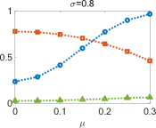
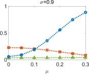
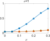
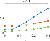
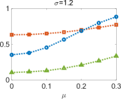
Figure 2.2: Powers of $A^{[m]}_{N}$ for $\mu\in[0,0.3]$ and $\sigma\in\{0.8,0.9,1,1.1,1.2\}$.

(blue circle: $m=1$, red square: $m=2$, green triangle: $m=3$)

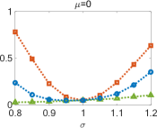
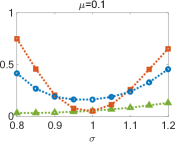
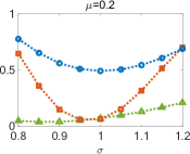
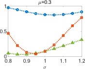
Figure 2.3: Powers of $A^{[m]}_{N}$ for $\sigma\in[0.8,1.2]$ and $\mu\in\{0,0.1,0.2,0.3\}$.

(blue circle: $m=1$, red square: $m=2$, green triangle: $m=3$)

Second, we assume the skew-normal distribution with density

$$\frac{2}{\omega}\phi\Bigl{(}\frac{x-\xi}{\omega}\Bigr{)}\Phi\Bigl{(}\alpha\frac{x-\xi}{\omega}\Bigr{)}$$ (40)

as alternatives (Azzalini, 1985), where $\phi$ and $\Phi$ are the probability density function and the cumulative distribution function of the standard normal distribution, respectively. The mean and the variance of the skew-normal distribution are

$$\mu=\xi+\omega\delta\sqrt{\frac{2}{\pi}}\quad\mbox{and}\quad\sigma^{2}=\omega^{2}\Bigl{(}1-\frac{2\delta^{2}}{\pi}\Bigr{)}\quad\mbox{with}\quad\delta=\frac{\alpha}{\sqrt{1+\alpha^{2}}},$$

respectively. The null hypothesis (the standard normal distribution) corresponds to the case $\xi=0$, $\omega=1$, and $\alpha=0$. For arbitrary $\alpha$, $(\mu,\sigma)=(0,1)$ is equivalent to

$$(\xi,\omega)=\biggl{(}{-\omega\delta\sqrt{\frac{2}{\pi}},\frac{1}{\sqrt{1-2\delta^{2}/\pi}}}\biggr{)}.$$

The powers of $A_{N}^{[1]}$, $A_{N}^{[2]}$ and $A_{N}^{[3]}$ are summarized in Figure 2.4. Note that for skewed normal distribution the power functions $(\alpha,\mu)$ and $(-\alpha,-\mu)$ are identical.

From the figures, we see that, when $\sigma=1$ and the absolute value of $\mu$ is large, $A_{N}^{[1]}$ is superior to $A_{N}^{[2]}$, and when $\mu=0$ and $\sigma$ is away from 1, $A_{N}^{[2]}$ is superior to $A_{N}^{[1]}$. This is similar to what has already been observed in Figures 2.2 and 2.3, and is consistent with the findings in Durio and Nikitin (2016), where they showed that, even after adjusting the mean and the variance, integrated statistics have considerable statistical power.

Moreover, when $|\alpha|$ increases, $A_{N}^{[3]}$ begins to perform better, and can detect $\alpha\neq 0$ even when $(\mu,\sigma)=(0,1)$. Indeed, when $(\mu,\sigma)\approx(0,1)$, $A_{N}^{[3]}$ has considerable power when compared with $A_{N}^{[1]}$ and $A_{N}^{[2]}$.

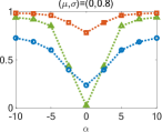
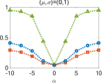
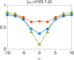
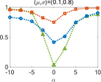
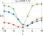
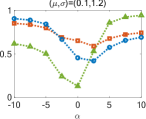
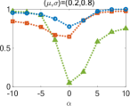
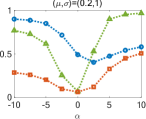
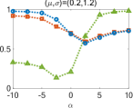
Figure 2.4: Powers of $A^{[m]}_{N}$ under skew-normal distributions with index $\alpha$, $\mu\in\{0,0.1,0.2\}$ and $\sigma\in\{0.8,1,1.2\}$.

(blue circle: $m=1$, red square: $m=2$, green triangle: $m=3$)

2.6 Two-sample test statistic

For the original Anderson-Darling statistic, Pettitt (1976) proposed a two-sample statistic for testing equality of two empirical distributions. Given two distribution functions $F^{(\ell)}$, $\ell=1,2$, assume that two i.i.d. samples $X^{(\ell)}_{1},\ldots,X^{(\ell)}_{N_{\ell}}$ from $F^{(\ell)}$ are available. The merged dataset of $X^{(\ell)}_{j}$’s is denoted by $Y_{1},\ldots,Y_{N}$, $N=N_{1}+N_{2}$. Let

$$R^{(\ell)}_{j}=\sharp\left(i\mid Y_{i}\leqslant X^{(\ell)}_{j}\right)$$

be the rank of $X^{(\ell)}_{j}$ in the whole dataset $Y_{1},\ldots,Y_{N}$.

Then, the $m$-fold integrated two-sample Anderson-Darling statistic for testing $H_{0}:F^{(1)}=F^{(2)}$ against $H_{1}:F^{(1)}\neq F^{(2)}$ is given by

$$\widetilde{A}^{\,\,[m]}_{N_{1},N_{2}}=\frac{N_{1}N_{2}}{N^{2}}\sum_{1\leqslant i<N}\frac{\bigl{(}{B^{(1)}_{i}-B^{(2)}_{i}}\bigr{)}^{2}}{\left(\frac{i}{N}\bigl{(}{1-\frac{i}{N}}\bigr{)}\right)^{m}},$$ (41)

where

$$B^{(\ell)}_{i} =\frac{1}{N_{\ell}}\sum_{1\leqslant j\leqslant N_{\ell}}\frac{\bigl{(}{\frac{i}{N}-\frac{1}{N}R^{(\ell)}_{j}}\bigr{)}^{m-1}}{(m-1)!}\mathds{1}\bigl{(}{R^{(\ell)}_{j}\leqslant i}\bigr{)}$$

$$\qquad-\frac{1}{N_{\ell}}\sum_{0\leqslant k<m}P_{k}^{(-m)}\bigl{(}{\tfrac{i}{N}}\bigr{)}\sum_{1\leqslant j\leqslant N_{\ell}}P_{k}\Bigl{(}{\tfrac{R^{(\ell)}_{j}}{N}}\Bigr{)}.$$

To prove (41), note first that the $m$-fold GAD statistic for testing

$$H_{0}:F=F_{0}\quad\mbox{vs.}\quad H_{1}:F\neq F_{0}$$

without assuming that $F_{0}$ is the uniform distribution on $[0,1]$ is given as

$$A^{[m]}_{N}=N\int_{-\infty}^{\infty}\frac{\bigl{(}{\frac{1}{\sqrt{N}}B^{[m]}_{N}(x;F_{0};F_{N})}\bigr{)}^{2}}{\left(F_{0}(x)(1-F_{0}(x))\right)^{m}}\,\mathrm{d}F_{0}(x),$$

where

$$\frac{1}{\sqrt{N}}\,B^{[m]}_{N}(x;F_{0};F_{N})= \int_{-\infty}^{x}\frac{(F_{0}(x)-F_{0}(t))^{m-1}}{(m-1)!}\,\mathrm{d}F_{N}(t)$$

$$-\sum_{0\leqslant k<m}P_{k}^{(-m)}(F_{0}(x))\int_{-\infty}^{\infty}P_{k}(F_{0}(x))\,\mathrm{d}F_{N}(x).$$

Let $F_{N_{\ell}}^{(\ell)}$ be the underlying empirical distribution function of $X^{(\ell)}_{1},\ldots,X^{(\ell)}_{N_{\ell}}$ for $\ell=1,2$. Denote by $F_{N}$ the empirical distribution function of the merged data $Y_{1},\ldots,Y_{N}$, $N=N_{1}+N_{2}$. Obviously,

$$F_{N}(x)=\frac{N_{1}F^{(1)}_{N_{1}}(x)+N_{2}F^{(2)}_{N_{2}}(x)}{N}.$$

The two-sample Anderson-Darling statistic is defined by

$$\widetilde{A}^{\,\,[m]}_{N_{1},N_{2}}=\frac{N_{1}N_{2}}{N}\int_{-\infty}^{\infty}\frac{\left(\frac{1}{\sqrt{N_{1}}}B^{[m]}_{N_{1}}\bigl{(}{x;F_{N};F^{(1)}_{N_{1}}}\bigr{)}-\frac{1}{\sqrt{N_{2}}}B^{[m]}_{N_{2}}\bigl{(}{x;F_{N};F^{(2)}_{N_{2}}}\bigr{)}\right)^{2}}{\left(F_{N}(x)(1-F_{N}(x))\right)^{m}}\,\mathrm{d}F_{N}(x).$$

Since $F_{N}(X^{(\ell)}_{j})=\frac{1}{N}R^{(\ell)}_{j}$, a simple calculation then yields the result (41).

As Pettitt (1976) proved, the original Anderson-Darling statistic has the same limiting null distribution as the one-sided case. This holds for the general $m$ as well, but the details are omitted here.

2.7 The MGF of the limit law $A^{[m]}$

By the expansion (38), we see that the MGF of the limit law $A^{[m]}$ has the infinite product representation

$$\mathbb{E}\bigl{(}{e^{sA^{[m]}}}\bigr{)}=\prod_{k\geqslant 1}\frac{1}{\sqrt{1-\frac{2s}{\lambda_{k}}}}\quad\text{where}\quad\lambda_{k}:=k(k+1)\cdots(k+2m+1).$$

This expression holds for complex $s$ except for the branch-cut $[\frac{1}{2}\lambda_{1},\infty)$. It is known that

$$\mathbb{E}\bigl{(}{e^{sA^{[1]}}}\bigr{)}=\sqrt{\frac{-2\pi s}{\cos\frac{\pi}{2}\sqrt{1+8s}}}.$$ (42)

We derive a similar representation for all $m\geqslant 1$.

Theorem 2.4.

Let $\eta_{j}$ ($0\leqslant j<m$) represent the zeros of the polynomial equation (in $z$)

$$\prod_{0\leqslant j<m}\left(z-(j+\tfrac{1}{2})^{2}\right)-2s=0.$$ (43)

Then for $m\geqslant 1$

$$\mathbb{E}\bigl{(}{e^{sA^{[m]}}}\bigr{)}=\sqrt{\frac{(-2\pi s)^{m}}{1!2!\cdots(2m-1)!}\prod_{0\leqslant j<m}\frac{1}{\cos\bigl{(}{\pi\sqrt{\eta_{j}}}\bigr{)}}},$$ (44)

where the square-root denotes the principal branch.

The finite product representation (44) is preferable for most analytic or numerical purposes. For example, the distribution function of $A^{[m]}$ can be computed by the following formula

$$\mathbb{P}\bigl{(}{A^{[m]}>x}\bigr{)}=\text{\scalebox{0.9}{$\frac{1}{\pi}$}}\sum_{k\geqslant 1}(-1)^{k-1}\int_{\frac{1}{2}\lambda_{2k-1}}^{\frac{1}{2}\lambda_{2k}}\frac{e^{-xs}}{s\sqrt{\bigl{|}\mathbb{E}\bigl{(}{e^{sA^{[m]}}}\bigr{)}\bigr{|}}}\,\mathrm{d}s,$$ (45)

which may be called the Smirnov-Slepian formula; see Smirnov (1937); Slepian (1958) for the original papers where such a technique was introduced. See also Matsui and Takemura (2008) and Deheuvels and Martynov (2008) for other applications. In the above formula, we see that effective numerical procedures such as (44) are crucial in computing the tails to high precision.

In particular, when $m=1$, the solution to $\eqref{poly-eq}$ is obviously given by $\eta_{0}=\frac{1}{4}+2s$, so we obtain (42). When $m=2$, the solutions to (43) are $\frac{5}{4}\pm\sqrt{1+2s}$, so we obtain the identity

$$\begin{split}&\prod_{k\geqslant 1}\frac{1}{\sqrt{1-\frac{2s}{k(k+1)(k+2)(k+3)}}}\\ &\qquad=\frac{\pi s}{\sqrt{3\cos\left(\frac{\pi}{2}\sqrt{5-4\sqrt{1+2s}}\right)\cos\left(\frac{\pi}{2}\sqrt{5+4\sqrt{1+2s}}\right)}}.\end{split}$$ (46)

A very different construction based on Jacobi polynomials leading to an MGF of the same form but with $s\mapsto 6s$ can be found in Deheuvels and Martynov (2008). For $m=3$,

$$\begin{split}&\prod_{k\geqslant 1}\frac{1}{\sqrt{1-\frac{2s}{k(k+1)(k+2)(k+3)(k+4)(k+5)}}}\\ &\qquad=\frac{(\pi s)^{3/2}}{\sqrt{-4320\cos\left(\pi\sqrt{\eta_{1}}\right)\cosh\left(\pi\sqrt{\eta_{2}}\right)\cosh\left(\pi\sqrt{\eta_{3}}\right)}}\end{split}$$ (47)

where $\eta:=\sqrt[3]{27s+80+3\sqrt{81s^{2}+480s-1728})}$ and

$$\eta_{1} :=\frac{1}{12\eta}\left(4\eta^{2}+35\eta+112\right),$$

$$\eta_{2} :=\frac{1}{12\eta}\left(4e^{-\pi i/3}\eta^{2}-35\eta+112e^{\pi i/3}\right),$$

$$\eta_{3} :=\frac{1}{12\eta}\left(4e^{\pi i/3}\eta^{2}-35\eta+112e^{-\pi i/3}\right).$$

While the exact expressions readily become lengthy for higher values of $m$, numerical evaluation is rather straightforward once the value of $s$ is specified.

Lemma 2.7.

Let $\zeta_{j}(s)$, $0\leqslant j<2m$, denote the zeros of the polynomials $z(z+1)\cdots(z+2m-1)-2s$:

$$z(z+1)\cdots(z+2m-1)-2s=\prod_{0\leqslant j<2m}\left(z-\zeta_{j}(s)\right).$$ (48)

Then

$$\mathbb{E}\bigl{(}{e^{sA^{[m]}}}\bigr{)}=\sqrt{\prod_{0\leqslant j<2m}\frac{\Gamma(1-\zeta_{j}(s))}{j!}}.$$ (49)

Proof.

By (48)

$$1-\frac{2s}{k(k+1)\cdots(k+2m-1)}=\prod_{0\leqslant j<2m}\frac{k-\zeta_{j}(s)}{k+j}=\prod_{0\leqslant j<2m}\frac{1-\frac{\zeta_{j}(s)}{k}}{1+\frac{j}{k}}.$$

Note that

$$-\sum_{0\leqslant j<2m}\zeta_{j}(s)=[z^{2m-1}]\prod_{0\leqslant j<2m}(z+j)=m(2m-1)=\sum_{0\leqslant j<2m}j,$$ (50)

where $[z^{m}]f(z)$ denotes the coefficient of $z^{m}$ in the Taylor expansion of $f(z)$. Using the identity (50) and the infinite product representation of the Gamma function

$$\Gamma(1+s)e^{\gamma s}=\prod_{k\geqslant 1}\frac{e^{\frac{s}{k}}}{1+\frac{s}{k}},$$

we then have

$$\prod_{k\geqslant 1}\frac{1}{1-\frac{2s}{k(k+1)\cdots(k+2m-1)}} =\prod_{k\geqslant 1}\prod_{0\leqslant j<2m}\frac{\left(1+\frac{j}{k}\right)e^{-\frac{j}{k}}}{\bigl{(}{1-\frac{\zeta_{j}(s)}{k}}\bigr{)}e^{-\frac{\zeta_{j}(s)}{k}}}$$

$$=\prod_{0\leqslant j<2m}\frac{\Gamma(1-\zeta_{j}(s))e^{-\gamma\zeta_{j}(s)}}{\Gamma(j+1)e^{j\gamma}}$$

$$=\prod_{0\leqslant j<2m}\frac{\Gamma(1-\zeta_{j}(s))}{j!}.$$

This proves (49). ∎

Proof of Theorem 2.4..

Note that the roots of the equation (48) are symmetric with respect to $-m+\frac{1}{2}$, namely, if $-m+\frac{1}{2}+\zeta$ is a root of the equation (48), then $-m+\frac{1}{2}-\zeta$ is also a root. Thus we can regroup the zeros in pairs and use the factorization

$$\Gamma\bigl{(}{m+\tfrac{1}{2}-\zeta}\bigr{)}\Gamma\bigl{(}{m+\tfrac{1}{2}+\zeta}\bigr{)}$$

$$\qquad=\Gamma\bigl{(}{-m+\tfrac{1}{2}-\zeta}\bigr{)}\Gamma\bigl{(}{m+\tfrac{1}{2}+\zeta}\bigr{)}\prod_{0\leqslant\ell<2m}\left(-m+\tfrac{1}{2}-\zeta+\ell\right),$$

which equals, by Euler’s reflection formula

$$\Gamma(s)\Gamma(1-s)=\frac{\pi}{\sin\pi s},$$

and (48), to

$$\Gamma\bigl{(}{m+\tfrac{1}{2}-\zeta}\bigr{)}\Gamma\bigl{(}{m+\tfrac{1}{2}+\zeta}\bigr{)}=\frac{2\pi s}{\sin\bigl{(}{\pi(m+\tfrac{1}{2}+\zeta)}\bigr{)}}=\frac{(-1)^{m}2\pi s}{\cos(\pi\zeta)}.$$

Now if we replace $x$ in the equation $x\cdots(x+2m-1)=2s$ by $x\mapsto-m+\tfrac{1}{2}+z$, then equation (48) becomes

$$\prod_{0\leqslant j<m}\left(z^{2}-(-m+\tfrac{1}{2}+j)^{2}\right)=2s,$$

which is equivalent to

$$\prod_{0\leqslant j<m}\left(z^{2}-(j+\tfrac{1}{2})^{2}\right)=2s.$$

Thus it suffices to consider the equation (43)

$$\prod_{0\leqslant j<m}\left(z-(j+\tfrac{1}{2})^{2}\right)=2s.$$

It then follows that

$$\prod_{0\leqslant j<2m}\Gamma(1-\zeta_{j}(s))=\prod_{0\leqslant j<m}\frac{(-1)^{m}2\pi s}{\cos\bigl{(}{\pi\sqrt{\eta_{j}}}\bigr{)}}.$$

This proves (44). ∎

3 The generalized Watson statistics

We follow the same approach developed above and examine a generalization of Watson’s statistic by the same iterated empirical measures.

3.1 A new class of Watson statistics

Let $X_{1},\ldots,X_{N}$ be an i.i.d. sequence on $[0,1)=\{\{x\}\,|\,x\in\mathbb{R}\}$, where $\{x\}=x\bmod 1$ denotes the fractional part of $x$. Here the $X_{i}$’s are referred to as “circular data” or “directional data”. Watson (1961)’s statistic to test the uniformity of $X_{i}$’s on $[0,1)$ is defined as

$$U_{N}=\int_{0}^{1}\,\vbox{\hrule height=0.6pt\kern 1.07639pt\hbox{\kern-1.99997pt$B$\kern-1.00006pt} }_{N}(x)^{2}\,\mathrm{d}x,\quad\,\vbox{\hrule height=0.6pt\kern 1.07639pt\hbox{\kern-1.99997pt$B$\kern-1.00006pt} }_{N}(x)=B_{N}(x)-\int_{0}^{1}B_{N}(x)\,\mathrm{d}x,$$ (51)

where $B_{N}(x)=\sqrt{N}(F_{N}(x)-x)=\sqrt{N}\int_{0}^{1}(\mathds{1}_{\{t\leqslant x\}}-x)\,\mathrm{d}F_{N}(t)$ as before.

The generalized Watson (GW) statistics we propose here are defined similarly as the GAD statistics. In particular, the correction term $-\int_{0}^{1}B_{N}(x)\,\mathrm{d}x$ in (51) makes the statistic invariant with respect to the choice of the origin of the data $X_{i}\mapsto\{X_{i}+a\}$ ($a$ is a constant), and the reflection of the data $X_{i}\mapsto\{-X_{i}\}$; see Corollary 3.1. Such a correction will also be incorporated in our generalized Watson statistics.

Let $\,\vbox{\hrule height=0.6pt\kern 1.07639pt\hbox{\kern-1.99997pt$B$\kern-1.00006pt} }^{[1]}_{N}(x)=\,\vbox{\hrule height=0.6pt\kern 1.07639pt\hbox{\kern-1.99997pt$B$\kern-1.00006pt} }_{N}(x)$ and

$$\,\vbox{\hrule height=0.6pt\kern 1.07639pt\hbox{\kern-1.99997pt$B$\kern-1.00006pt} }^{[m+1]}_{N}(x) =\int_{0}^{x}\,\vbox{\hrule height=0.6pt\kern 1.07639pt\hbox{\kern-1.99997pt$B$\kern-1.00006pt} }^{[m]}_{N}(t)\,\mathrm{d}t-\int_{0}^{1}\int_{0}^{x}\,\vbox{\hrule height=0.6pt\kern 1.07639pt\hbox{\kern-1.99997pt$B$\kern-1.00006pt} }^{[m]}_{N}(t)\,\mathrm{d}t\,\mathrm{d}x$$

$$=\int_{0}^{x}\,\vbox{\hrule height=0.6pt\kern 1.07639pt\hbox{\kern-1.99997pt$B$\kern-1.00006pt} }^{[m]}_{N}(t)\,\mathrm{d}t-\int_{0}^{1}(1-t)\,\vbox{\hrule height=0.6pt\kern 1.07639pt\hbox{\kern-1.99997pt$B$\kern-1.00006pt} }^{[m]}_{N}(t)\,\mathrm{d}t\qquad(m\geqslant 1).$$ (52)

Then $\int_{0}^{1}\,\vbox{\hrule height=0.6pt\kern 1.07639pt\hbox{\kern-1.99997pt$B$\kern-1.00006pt} }^{[m]}_{N}(t)\,\mathrm{d}t=0$ and $\,\vbox{\hrule height=0.6pt\kern 1.07639pt\hbox{\kern-1.99997pt$B$\kern-1.00006pt} }^{[m]}_{N}(x)$ is an $m$-fold iterated integral of the empirical measure $\,\mathrm{d}F_{N}$ with mean zero. Thus we define the GW statistic as

$$U^{[m]}_{N}:=\int_{0}^{1}\,\vbox{\hrule height=0.6pt\kern 1.07639pt\hbox{\kern-1.99997pt$B$\kern-1.00006pt} }^{[m]}_{N}(x)^{2}\,\mathrm{d}x.$$

Normalized Bernoulli polynomials.

As in the case of the GAD statistic, $\,\vbox{\hrule height=0.6pt\kern 1.07639pt\hbox{\kern-1.99997pt$B$\kern-1.00006pt} }^{[m]}_{N}(x)$ can be expressed in terms of a class of template functions. For that purpose, we introduce the following polynomials. For $m\geqslant 1$, let $b_{m}(y)$ be a polynomial in $y$ of degree $m$ satisfying

$$b_{m}(y+1)=b_{m}(y)+\frac{y^{m-1}}{(m-1)!}\quad\text{and}\quad\int_{0}^{1}b_{m}(y)\,\mathrm{d}y=0.$$ (53)

It turns out that the polynomial $m!b_{m}(y)$ is identical to Bernoulli polynomial of order $m$. Alternatively, $b_{m}(y)$ can be computed recursively by

$$b_{m+1}(y)=\int_{0}^{y}b_{m}(t)\,\mathrm{d}t-\int_{0}^{1}(1-t)b_{m}(t)\,\mathrm{d}t,$$ (54)

with $b_{0}(y)=1$. In particular,

$b_{0}(y)$	$b_{1}(y)$	$b_{2}(y)$	$b_{3}(y)$	$b_{4}(y)$
1	$y-\frac{1}{2}$	$\frac{y^{2}}{2}-\frac{y}{2}+\frac{1}{12}$	$\frac{y^{3}}{6}-\frac{y^{2}}{4}+\frac{y}{12}$	$\frac{y^{4}}{24}-\frac{y^{3}}{12}+\frac{y^{2}}{24}-\frac{1}{720}$

The generating function of $b_{m}(y)$ is

$$V(z;x)=\sum_{m\geqslant 0}b_{m}(x)z^{m}=\frac{ze^{xz}}{e^{z}-1}\qquad(|z|<2\pi),$$ (55)

and the Fourier series is given, for $m\geqslant 1$, by

$$b_{m}(x)=-2\sum_{k\geqslant 1}\frac{\cos\bigl{(}2k\pi x-\frac{m\pi}{2}\bigr{)}}{(2k\pi)^{m}}\qquad(0<x<1);$$ (56)

see (Abramowitz and Stegun, 1964, p. 805). Another property we need is $b_{m}(1-x)=(-1)^{m}b_{m}(x)$. Note that, from (53) and (54), the generating function satisfies

$$\left\{\begin{aligned} &\int_{0}^{1}V(z;y)\,\mathrm{d}y=1,\\ &z^{-1}(V(z;y)-1)=\int_{0}^{y}V(z;t)\,\mathrm{d}t-\int_{0}^{1}(1-t)V(z;t)\,\mathrm{d}t.\end{aligned}\right.$$ (57)

The template functions.

Let

$$\bar{\tau}_{m}(t;x) =\frac{(x-t)^{m-1}}{(m-1)!}\mathds{1}_{\{t\leqslant x\}}+(-1)^{m-1}b_{m}(t-x)$$

$$=(-1)^{m-1}b_{m}(t-x+1)\mathds{1}_{\{t\leqslant x\}}+(-1)^{m-1}b_{m}(t-x)\mathds{1}_{\{t>x\}}.$$ (58)

The $\,\vbox{\hrule height=0.6pt\kern 1.07639pt\hbox{\kern-1.99997pt$B$\kern-1.00006pt} }_{N}^{[m]}(x)$ are linked to the template functions by the following integral representation.

Lemma 3.1.

For $m\geqslant 1$

$$\,\vbox{\hrule height=0.6pt\kern 1.07639pt\hbox{\kern-1.99997pt$B$\kern-1.00006pt} }^{[m]}_{N}(x)=\int_{0}^{1}\bar{\tau}_{m}(t;x)\,\mathrm{d}F_{N}(x).$$ (59)

Proof.

Substituting (59) into the right-hand side of (52), we obtain

$$\,\vbox{\hrule height=0.6pt\kern 1.07639pt\hbox{\kern-1.99997pt$B$\kern-1.00006pt} }^{[m+1]}_{N}(x) =\int_{0}^{x}\,\vbox{\hrule height=0.6pt\kern 1.07639pt\hbox{\kern-1.99997pt$B$\kern-1.00006pt} }^{[m]}_{N}(u)\,\mathrm{d}u-\int_{0}^{1}(1-u)\,\vbox{\hrule height=0.6pt\kern 1.07639pt\hbox{\kern-1.99997pt$B$\kern-1.00006pt} }^{[m]}_{N}(u)\,\mathrm{d}u$$

$$=\int_{0}^{x}\int_{0}^{1}\bar{\tau}_{m}(t;u)\,\mathrm{d}F_{N}(t)\,\mathrm{d}u-\int_{0}^{1}(1-u)\int_{0}^{1}\bar{\tau}_{m}(t;u)\,\mathrm{d}F_{N}(t)\,\mathrm{d}u$$

$$=\int_{0}^{1}\,\mathrm{d}F_{N}(t)\int_{0}^{1}\left(\mathds{1}_{\{u\leqslant x\}}-(1-u)\right)\bar{\tau}_{m}(t;u)\,\mathrm{d}u$$

$$=\int_{0}^{1}\,\mathrm{d}F_{N}(t)\int_{0}^{1}\left(u\mathds{1}_{\{u\leqslant x\}}-(1-u)\mathds{1}_{\{u>x\}}\right)\bar{\tau}_{m}(t;u)\,\mathrm{d}u.$$

It suffices, by induction, to prove that

$$(-1)^{m-1}\int_{0}^{1}\bigl{(}{u\mathds{1}_{\{u\leqslant x\}}-(1-u)\mathds{1}_{\{u>x\}}}\bigr{)}\bar{\tau}_{m}(t;u)\,\mathrm{d}u=-(-1)^{m}\bar{\tau}_{m+1}(t;x).$$ (60)

By the definition of the generating function (55), $b_{m}(x)=[z^{m}]V(z;x)$ and thus $\bar{\tau}_{m}(t;x)$ in (58) can be written as

$$\bar{\tau}_{m}(t;x)=(-1)^{m-1}[z^{m}]\bigl{(}V(z;t-x+1)\mathds{1}_{\{t\leqslant x\}}+V(z;t-x)\mathds{1}_{\{t>x\}}\bigr{)}.$$ (61)

With this relation, together with (57), the left-hand side of (60) becomes

$$[z^{m}]\int_{0}^{1}(u\mathds{1}_{\{u\leqslant x\}}-(1-u)\mathds{1}_{\{u>x\}})\bigl{(}V(z;t-u+1)\mathds{1}_{\{t\leqslant u\}}+V(z;t-u)\mathds{1}_{\{t>u\}}\bigr{)}\,\mathrm{d}u$$

$$=[z^{m}]\biggl{\{}\mathds{1}_{\{t\leqslant x\}}\int_{t}^{x}uV(z;t-u+1)\,\mathrm{d}u-\int_{x\vee t}^{1}(1-u)V(z;t-u+1)\,\mathrm{d}u$$

$$\qquad\quad\ \ +\int_{0}^{x\wedge t}uV(z;t-u)\,\mathrm{d}u-\mathds{1}_{\{t>x\}}\int_{x}^{t}(1-u)V(z;t-u)\,\mathrm{d}u\biggr{\}}$$

$$=\begin{cases}\displaystyle[z^{m}]\left\{-z^{-1}V(z;t-x+1)+t+z^{-1}\right\}&(t\leqslant x),\\ \displaystyle[z^{m}]\left(-z^{-1}V(z;t-x)-(1-t)+z^{-1}\right)&(t>x)\end{cases}$$

$$=-[z^{m+1}]\bigl{(}V(z;t-x+1)\mathds{1}_{\{t\leqslant x\}}+V(z;t-x)\mathds{1}_{\{t>x\}}\bigr{)}$$

$$=-(-1)^{m}\bar{\tau}_{m+1}(t;x),$$

which proves (60) and completes the proof of the lemma. ∎

Following a similar construction principle used for GAD statistic where the template functions are orthogonal to eigenfunctions of lower degrees, we propose the truncated version of the template function

$$\bar{\tau}^{*}_{m}(t;x)=\bar{\tau}_{m}(t;x)-2\sum_{1\leqslant k<m}\frac{1}{(2k\pi)^{m}}\cos\Bigl{(}2k\pi(t-x)+\text{\scalebox{0.9}{$\frac{m\pi}{2}$}}\Bigr{)},$$ (62)

(compare (10)) and define the truncated version of the generalized Watson statistics

$$U^{*[m]}_{N}=\int_{0}^{1}\,\vbox{\hrule height=0.6pt\kern 1.07639pt\hbox{\kern-1.99997pt$B$\kern-1.00006pt} }^{*[m]}_{N}(x)^{2}\,\mathrm{d}x,\quad\,\vbox{\hrule height=0.6pt\kern 1.07639pt\hbox{\kern-1.99997pt$B$\kern-1.00006pt} }^{*[m]}_{N}(x)=\int_{0}^{1}\bar{\tau}^{*}_{m}(t;x)\,\mathrm{d}F_{N}(x);$$

see also (68).

The first few $\bar{\tau}^{*}_{m}$ are plotted in Figure 3.1.

$\bar{\tau}^{*}_{1}(t;x_{0})$	$\bar{\tau}^{*}_{2}(t;x_{0})$
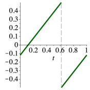
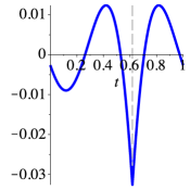
$\bar{\tau}^{*}_{3}(t;x_{0})$	$\bar{\tau}^{*}_{4}(t;x_{0})$

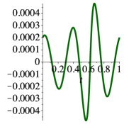
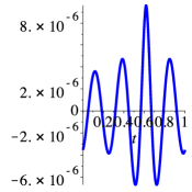
Figure 3.1: Template functions $\bar{\tau}^{*}_{m}(\cdot;x_{0})$ for the generalized Watson statistics for $1\leqslant m\leqslant 4$; here $x_{0}=\frac{\sqrt{5}-1}{2}$, the reciprocal of the golden ratio.

Corollary 3.1.

The statistics $U_{N}^{[m]}$ and $U_{N}^{*[m]}$ are well-defined and independent of the choice of the origin. They are invariant with respect the sign change $X_{i}\mapsto\{-X_{i}\}=1-X_{i}$.

Proof.

Consider first $U_{N}^{[m]}$. If $X_{i}\mapsto\{X_{i}+a\}$, $i=1,\ldots,N$, then

$$\,\vbox{\hrule height=0.6pt\kern 1.07639pt\hbox{\kern-1.99997pt$B$\kern-1.00006pt} }^{[m]}_{N}(x)=\text{\scalebox{0.9}{$\frac{1}{\sqrt{N}}$}}\sum_{1\leqslant i\leqslant N}\bar{\tau}_{m}(X_{i};x)\mapsto \text{\scalebox{0.9}{$\frac{1}{\sqrt{N}}$}}\sum_{1\leqslant i\leqslant N}\bar{\tau}_{m}(\{X_{i}+a\};x)$$

$$=\text{\scalebox{0.9}{$\frac{1}{\sqrt{N}}$}}\sum_{1\leqslant i\leqslant N}\bar{\tau}_{m}(X_{i};\{x-a\})$$

$$=\,\vbox{\hrule height=0.6pt\kern 1.07639pt\hbox{\kern-1.99997pt$B$\kern-1.00006pt} }^{[m]}_{N}(\{x-a\}).$$

Thus

$$U^{[m]}_{N}=\int_{0}^{1}\,\vbox{\hrule height=0.6pt\kern 1.07639pt\hbox{\kern-1.99997pt$B$\kern-1.00006pt} }^{[m]}_{N}(x)^{2}\,\mathrm{d}x\mapsto\int_{0}^{1}\,\vbox{\hrule height=0.6pt\kern 1.07639pt\hbox{\kern-1.99997pt$B$\kern-1.00006pt} }^{[m]}_{N}(\{x-a\})^{2}\,\mathrm{d}x=U^{[m]}_{N},$$

where we used the relation

$$(\{X_{i}+a\}-x)-(X_{i}-\{x-a\}) =-(X_{i}+a-\{X_{i}+a\})-(x-a-\{x-a\})$$

$$=0\bmod 1.$$

On the other hand, if $X_{i}\mapsto\{-X_{i}\}=1-X_{i}$, $i=1,\ldots,N$, then

$$\,\vbox{\hrule height=0.6pt\kern 1.07639pt\hbox{\kern-1.99997pt$B$\kern-1.00006pt} }^{[m]}_{N}(x)=\text{\scalebox{0.9}{$\frac{1}{\sqrt{N}}$}}\sum_{1\leqslant i\leqslant N}\bar{\tau}_{m}(X_{i};x)\mapsto \text{\scalebox{0.9}{$\frac{1}{\sqrt{N}}$}}\sum_{1\leqslant i\leqslant N}\bar{\tau}_{m}(1-X_{i};x)$$

$$=\text{\scalebox{0.9}{$\frac{1}{\sqrt{N}}$}}\sum_{1\leqslant i\leqslant N}(-1)^{m}\bar{\tau}_{m}(X_{i};1-x)$$

$$=(-1)^{m}\,\vbox{\hrule height=0.6pt\kern 1.07639pt\hbox{\kern-1.99997pt$B$\kern-1.00006pt} }^{[m]}_{N}(1-x).$$

It follows that

$$U^{[m]}_{N}=\int_{0}^{1}\,\vbox{\hrule height=0.6pt\kern 1.07639pt\hbox{\kern-1.99997pt$B$\kern-1.00006pt} }^{[m]}_{N}(x)^{2}\,\mathrm{d}x\mapsto\int_{0}^{1}\,\vbox{\hrule height=0.6pt\kern 1.07639pt\hbox{\kern-1.99997pt$B$\kern-1.00006pt} }^{[m]}_{N}(1-x)^{2}\,\mathrm{d}x=U^{[m]}_{N}.$$

The proof for $U_{N}^{*[m]}$ is similar. ∎

3.2 The limiting GW processes: KL expansions and covariance kernel

In this section, we examine the limiting distribution of the GW statistic under the null hypothesis $H_{0}$.

From their constructions, $U^{[m]}_{N}$ and $U^{*[m]}_{N}$ have almost the same eigenstructure. In this subsection, we mainly deal with the non-truncated version $U^{[m]}_{N}$. As in Sec. 2.3, we denote by $W(x)$ and $B(x)$ the Wiener process on $[0,1]$ and the Brownian bridge, respectively. Using the template functions $\bar{\tau}_{m}(t;x)$ in (58) and $\bar{\tau}^{*}_{m}(t;x)$ in (62), we now define the limiting GW processes

$$\,\vbox{\hrule height=0.6pt\kern 1.07639pt\hbox{\kern-1.99997pt$B$\kern-1.00006pt} }^{[m]}(x)=\int_{0}^{1}\bar{\tau}_{m}(t;x)\,\mathrm{d}W(t)=\int_{0}^{1}\bar{\tau}_{m}(t;x)\,\mathrm{d}B(t),$$ (63)

$$\,\vbox{\hrule height=0.6pt\kern 1.07639pt\hbox{\kern-1.99997pt$B$\kern-1.00006pt} }^{*[m]}(x)=\int_{0}^{1}\bar{\tau}^{*}_{m}(t;x)\,\mathrm{d}W(t)=\int_{0}^{1}\bar{\tau}^{*}_{m}(t;x)\,\mathrm{d}B(t).$$

Since the Brownian bridge $B(\cdot)$ is continuous on $[0,1]$, both $\,\vbox{\hrule height=0.6pt\kern 1.07639pt\hbox{\kern-1.99997pt$B$\kern-1.00006pt} }^{[m]}(\cdot)$ and $\,\vbox{\hrule height=0.6pt\kern 1.07639pt\hbox{\kern-1.99997pt$B$\kern-1.00006pt} }^{*[m]}(\cdot)$ are of the class $C^{m-1}$ on $[0,1]$.

We now describe the weak convergence of these processes in the functional spaces $L^{2}([0,1],\mu)$ and $L^{\infty}([0,1])$, the space of all essentially bounded functions on $[0,1]$.

Lemma 3.2.

Let $\mu$ be any finite measure on $[0,1]$. As $N\to\infty$, $\,\vbox{\hrule height=0.6pt\kern 1.07639pt\hbox{\kern-1.99997pt$B$\kern-1.00006pt} }^{[m]}_{N}(\cdot)\stackrel{{\scriptstyle d}}{{\to}}\,\vbox{\hrule height=0.6pt\kern 1.07639pt\hbox{\kern-1.99997pt$B$\kern-1.00006pt} }^{[m]}(\cdot)$ and $\,\vbox{\hrule height=0.6pt\kern 1.07639pt\hbox{\kern-1.99997pt$B$\kern-1.00006pt} }^{*[m]}_{N}(\cdot)\stackrel{{\scriptstyle d}}{{\to}}\,\vbox{\hrule height=0.6pt\kern 1.07639pt\hbox{\kern-1.99997pt$B$\kern-1.00006pt} }^{*[m]}(\cdot)$ in $L^{2}([0,1],\mu)$ and in $L^{\infty}([0,1])$, and $U^{[m]}_{N}\stackrel{{\scriptstyle d}}{{\to}}U^{[m]}$ and $U^{*[m]}_{N}\stackrel{{\scriptstyle d}}{{\to}}U^{*[m]}$, where

$$U^{[m]}=\int_{0}^{1}\,\vbox{\hrule height=0.6pt\kern 1.07639pt\hbox{\kern-1.99997pt$B$\kern-1.00006pt} }^{[m]}(x)^{2}\,\mathrm{d}x\quad\text{and}\quad U^{*[m]}=\int_{0}^{1}\,\vbox{\hrule height=0.6pt\kern 1.07639pt\hbox{\kern-1.99997pt$B$\kern-1.00006pt} }^{*[m]}(x)^{2}\,\mathrm{d}x.$$

Proof.

The stochastic map $x\mapsto B_{N}(x)=\sqrt{N}(F_{N}(x)-x)$ converges weakly to $B(\cdot)$ in both $L^{2}([0,1],\mu)$ and $L^{\infty}([0,1])$. $B^{[m]}(\cdot)$ and $B^{*[m]}(\cdot)$ in (63) are continuous in $B(\cdot)$ in both $L^{2}([0,1],\mu)$ and $L^{\infty}([0,1])$. The rest of the proof is similar to that of Lemma 2.4. ∎

We now clarify the covariances of the $\,\vbox{\hrule height=0.6pt\kern 1.07639pt\hbox{\kern-1.99997pt$B$\kern-1.00006pt} }^{[m]}(\cdot)$ and $\,\vbox{\hrule height=0.6pt\kern 1.07639pt\hbox{\kern-1.99997pt$B$\kern-1.00006pt} }^{*[m]}(\cdot)$, which are centered Gaussian processes on $[0,1]$.

Theorem 3.1.

For $m\geqslant 1$

$$\mathrm{Cov}\bigl{(}{\,\vbox{\hrule height=0.6pt\kern 1.07639pt\hbox{\kern-1.99997pt$B$\kern-1.00006pt} }^{[m]}(x),\,\vbox{\hrule height=0.6pt\kern 1.07639pt\hbox{\kern-1.99997pt$B$\kern-1.00006pt} }^{[m]}(y)}\bigr{)}=(-1)^{m-1}b_{2m}(|x-y|)=2\sum_{k\geqslant 1}\frac{\cos(2k\pi(x-y))}{(2k\pi)^{2m}},$$ (64)

$$\mathrm{Cov}\bigl{(}{\,\vbox{\hrule height=0.6pt\kern 1.07639pt\hbox{\kern-1.99997pt$B$\kern-1.00006pt} }^{*[m]}(x),\,\vbox{\hrule height=0.6pt\kern 1.07639pt\hbox{\kern-1.99997pt$B$\kern-1.00006pt} }^{*[m]}(y)}\bigr{)}=(-1)^{m-1}b_{2m}(|x-y|)-2\sum_{1\leqslant k<m}\frac{\cos(2k\pi(x-y))}{(2k\pi)^{2m}}.$$ (65)

In particular,

$$\mathrm{Var}\bigl{(}{\,\vbox{\hrule height=0.6pt\kern 1.07639pt\hbox{\kern-1.99997pt$B$\kern-1.00006pt} }^{[m]}(x)}\bigr{)}=(-1)^{m-1}b_{2m}(0),$$ (66)

$$\mathrm{Var}\bigl{(}{\,\vbox{\hrule height=0.6pt\kern 1.07639pt\hbox{\kern-1.99997pt$B$\kern-1.00006pt} }^{*[m]}(x)}\bigr{)}=(-1)^{m-1}b_{2m}(0)-2\sum_{1\leqslant k<m}\frac{1}{(2k\pi)^{2m}},$$

where the $(2m)!b_{2m}(0)$ are Bernoulli numbers.

Proof.

Assume without loss of generality that $0\leqslant x\leqslant y\leqslant 1$. We use again the generating function (55) of $b_{m}(x)$. By the representation for $\bar{\tau}_{m}(t;x)$ in (61), we see that the covariance function satisfies

$$\mathrm{Cov}\bigl{(}{\,\vbox{\hrule height=0.6pt\kern 1.07639pt\hbox{\kern-1.99997pt$B$\kern-1.00006pt} }^{[m]}(x),\,\vbox{\hrule height=0.6pt\kern 1.07639pt\hbox{\kern-1.99997pt$B$\kern-1.00006pt} }^{[m]}(y)}\bigr{)} =\int_{0}^{1}\bar{\tau}_{m}(t;x)\bar{\tau}_{m}(t;y)\,\mathrm{d}t$$

$$=[z^{m}w^{m}]\biggl{(}\int_{0}^{x}V(z;t-x+1)V(w;t-y+1)\,\mathrm{d}t$$

$$\qquad\qquad+\int_{x}^{y}V(z;t-x)V(w;t-y+1)\,\mathrm{d}t$$

$$\qquad\qquad+\int_{y}^{1}V(z;t-x)V(w;t-y)\,\mathrm{d}t\biggr{)}$$

$$=[z^{m}w^{m}]\frac{zw}{z+w}\left(\frac{e^{\Delta z}}{e^{z}-1}+\frac{e^{(1-\Delta)w}}{e^{w}-1}\right),$$

where $\Delta=y-x$. Now

$$\frac{zw}{z+w}\left(\frac{e^{\Delta z}}{e^{z}-1}+\frac{e^{(1-\Delta)w}}{e^{w}-1}\right) =\sum_{k\geqslant 0}\frac{wb_{k}(\Delta)z^{k}+zb_{k}(1-\Delta)w^{k}}{z+w}$$

$$=zw\sum_{k\geqslant 1}b_{k}(\Delta)\frac{z^{k-1}-(-w)^{k-1}}{z-(-w)}+1$$

$$=zw\sum_{k\geqslant 2}b_{k}(\Delta)\frac{z^{k-1}+(-w)^{k-1}}{z-(-w)}+1$$

$$=zw\sum_{k\geqslant 2}b_{k}(\Delta)\sum_{0\leqslant j\leqslant k-2}z^{j}(-w)^{k-j-2}+1.$$

It follows that when $x\leqslant y$, $\mathrm{Cov}\bigl{(}{\,\vbox{\hrule height=0.6pt\kern 1.07639pt\hbox{\kern-1.99997pt$B$\kern-1.00006pt} }^{[m]}(x),\,\vbox{\hrule height=0.6pt\kern 1.07639pt\hbox{\kern-1.99997pt$B$\kern-1.00006pt} }^{[m]}(y)}\bigr{)}=(-1)^{m-1}b_{2m}(\Delta)$. Similarly, when $x<y$, $\mathrm{Cov}\bigl{(}{\,\vbox{\hrule height=0.6pt\kern 1.07639pt\hbox{\kern-1.99997pt$B$\kern-1.00006pt} }^{[m]}(x),\,\vbox{\hrule height=0.6pt\kern 1.07639pt\hbox{\kern-1.99997pt$B$\kern-1.00006pt} }^{[m]}(y)}\bigr{)}=(-1)^{m-1}b_{2m}(-\Delta)$. We then conclude (64).

The proof of (65) is based on the identities

$$\int_{0}^{1}\bar{\tau}_{m}(t;x)\cos\Bigl{(}2k\pi(t-y)+\text{\scalebox{0.9}{$\frac{m\pi}{2}$}}\Bigr{)}\,\mathrm{d}t=\frac{\cos(2k\pi(x-y))}{(2k\pi)^{m}},$$

and

$$\begin{split}&\int_{0}^{1}\cos\Bigl{(}2k\pi(t-x)+\text{\scalebox{0.9}{$\frac{m\pi}{2}$}}\Bigr{)}\cos\Bigl{(}2\ell\pi(t-y)+\text{\scalebox{0.9}{$\frac{m\pi}{2}$}}\Bigr{)}\,\mathrm{d}t\\ &\qquad=\begin{cases}\text{\scalebox{0.9}{$\frac{1}{2}$}}\cos(2k\pi(x-y)),&k=\ell,\\ 0,&k\neq\ell,\end{cases}\end{split}$$ (67)

whose proofs are similar and omitted. ∎

Let $\psi_{0}(x)=1$, and $\psi_{2k-1}(x)=\sqrt{2}\sin(2k\pi x)$, $\psi_{2k}(x)=\sqrt{2}\cos(2k\pi x)$ for $k\geqslant 1$. Then, $\{\psi_{k}(x)\}_{k\geqslant 0}$ is a complete orthonormal basis of $L^{2}[0,1]$. For each $m\geqslant 1$, let

$$\psi^{[m]}_{2k-1}(x)=\sqrt{2}\sin\Bigl{(}2k\pi x-\text{\scalebox{0.9}{$\frac{m\pi}{2}$}}\Bigr{)}\quad\text{and}\quad\psi^{[m]}_{2k}(x)=\sqrt{2}\cos\Bigl{(}2k\pi x-\text{\scalebox{0.9}{$\frac{m\pi}{2}$}}\Bigr{)}.$$

Then $\{\psi^{[m]}_{k}(x)\}_{k\geqslant 0}$ also form an orthonormal basis. By expressing $\bar{\tau}_{m}(\cdot;x)$ in (58) as a Fourier series (56), and by expanding it on the basis $\psi_{k}(\cdot)$, we obtain the expansion

$$\bar{\tau}_{m}(t;x) =\sum_{k\geqslant 1}\frac{1}{(2k\pi)^{m}}\left(\psi^{[m]}_{2k-1}(x)\psi_{2k-1}(t)+\psi^{[m]}_{2k}(x)\psi_{2k}(t)\right)$$

$$=2\sum_{k\geqslant 1}\frac{1}{(2k\pi)^{m}}\cos\Bigl{(}2k\pi(t-x)+\text{\scalebox{0.9}{$\frac{m\pi}{2}$}}\Bigr{)},$$ (68)

and

$$\bar{\tau}^{*}_{m}(t;x)=\sum_{k\geqslant m}\frac{1}{(2k\pi)^{m}}\left(\psi^{[m]}_{2k-1}(x)\psi_{2k-1}(t)+\psi^{[m]}_{2k}(x)\psi_{2k}(t)\right).$$

By taking the stochastic integral $\int_{0}^{1}\,\mathrm{d}B(t)$ on both sides, we get the KL expansions

$$\,\vbox{\hrule height=0.6pt\kern 1.07639pt\hbox{\kern-1.99997pt$B$\kern-1.00006pt} }^{[m]}(x)=\sum_{k\geqslant 1}\frac{1}{(2k\pi)^{m}}\left(\psi^{[m]}_{2k-1}(x)\xi_{2k-1}+\psi^{[m]}_{2k}(x)\xi_{2k}\right),$$ (69)

$$\,\vbox{\hrule height=0.6pt\kern 1.07639pt\hbox{\kern-1.99997pt$B$\kern-1.00006pt} }^{*[m]}(x)=\sum_{k\geqslant m}\frac{1}{(2k\pi)^{m}}\left(\psi^{[m]}_{2k-1}(x)\xi_{2k-1}+\psi^{[m]}_{2k}(x)\xi_{2k}\right),$$ (70)

where

$$\xi_{j}=\int_{0}^{1}\psi_{j}(y)\,\mathrm{d}B(y)=\int_{0}^{1}\psi_{j}(y)\,\mathrm{d}W(y)\sim N(0,1)\ \ \rm i.i.d.$$ (71)

These KL expansions can again be justified by Mercer’s theorem.

Theorem 3.2.

Let $\xi_{k}$, $k\geqslant 0$, be i.i.d. standard Gaussian random variables defined by (71). For $m\geqslant 1$, (69) and (70) hold uniformly in $x\in[0,1]$ with probability 1, and both

$$U^{[m]}=\sum_{k\geqslant 1}\frac{\xi_{2k-1}^{2}+\xi_{2k}^{2}}{(2k\pi)^{2m}}\quad\text{and}\quad U^{*[m]}=\sum_{k\geqslant m}\frac{\xi_{2k-1}^{2}+\xi_{2k}^{2}}{(2k\pi)^{2m}}$$ (72)

converge with probability 1.

Proof.

Note that $\,\vbox{\hrule height=0.6pt\kern 1.07639pt\hbox{\kern-1.99997pt$B$\kern-1.00006pt} }^{[m]}(\cdot)$ is continuous on $[0,1]$. The covariance function of $\,\vbox{\hrule height=0.6pt\kern 1.07639pt\hbox{\kern-1.99997pt$B$\kern-1.00006pt} }^{[m]}(\cdot)$ is given in (64), which is continuous on $[0,1]\times[0,1]$. Moreover, by (66),

$$\int_{0}^{1}\mathrm{Cov}(\,\vbox{\hrule height=0.6pt\kern 1.07639pt\hbox{\kern-1.99997pt$B$\kern-1.00006pt} }^{[m]}(x),\,\vbox{\hrule height=0.6pt\kern 1.07639pt\hbox{\kern-1.99997pt$B$\kern-1.00006pt} }^{[m]}(x))\,\mathrm{d}x<\infty.$$

In addition, $\mathrm{Cov}\bigl{(}{\,\vbox{\hrule height=0.6pt\kern 1.07639pt\hbox{\kern-1.99997pt$B$\kern-1.00006pt} }^{[m]}(x),\,\vbox{\hrule height=0.6pt\kern 1.07639pt\hbox{\kern-1.99997pt$B$\kern-1.00006pt} }^{[m]}(y)}\bigr{)}$ satisfies the eigenequation

$$\int_{0}^{1}\mathrm{Cov}\bigl{(}{\,\vbox{\hrule height=0.6pt\kern 1.07639pt\hbox{\kern-1.99997pt$B$\kern-1.00006pt} }^{[m]}(x),\,\vbox{\hrule height=0.6pt\kern 1.07639pt\hbox{\kern-1.99997pt$B$\kern-1.00006pt} }^{[m]}(y)}\bigr{)}\psi^{[m]}_{k}(y)\,\mathrm{d}y=\frac{\psi^{[m]}_{k}(x)}{(2\lceil k/2\rceil\pi)^{2m}},\qquad k\geqslant 1.$$

The remaining proof then follows the same line as that of Theorem 2.3. The required results for $\,\vbox{\hrule height=0.6pt\kern 1.07639pt\hbox{\kern-1.99997pt$B$\kern-1.00006pt} }^{*[m]}(\cdot)$ and $U^{*[m]}$ are proved similarly. ∎

The covariance function for $B^{[m]}(\cdot)$ when $m=1$ is given explicitly by

$$\mathrm{Cov}\bigl{(}{\,\vbox{\hrule height=0.6pt\kern 1.07639pt\hbox{\kern-1.99997pt$B$\kern-1.00006pt} }^{[1]}(x),\,\vbox{\hrule height=0.6pt\kern 1.07639pt\hbox{\kern-1.99997pt$B$\kern-1.00006pt} }^{[1]}(y)}\bigr{)}=\text{\scalebox{0.9}{$\frac{1}{12}$}}-\text{\scalebox{0.9}{$\frac{1}{2}$}}|x-y|+\text{\scalebox{0.9}{$\frac{1}{2}$}}(x-y)^{2},$$

(see also (Watson, 1961, p. 111)), and when $m=2$

$$\mathrm{Cov}\bigl{(}{\,\vbox{\hrule height=0.6pt\kern 1.07639pt\hbox{\kern-1.99997pt$B$\kern-1.00006pt} }^{[2]}(x),\,\vbox{\hrule height=0.6pt\kern 1.07639pt\hbox{\kern-1.99997pt$B$\kern-1.00006pt} }^{[2]}(y)}\bigr{)}=\text{\scalebox{0.9}{$\frac{1}{720}$}}-\text{\scalebox{0.9}{$\frac{1}{24}$}}(x-y)^{2}+\text{\scalebox{0.9}{$\frac{1}{12}$}}|x-y|^{3}-\text{\scalebox{0.9}{$\frac{1}{24}$}}(x-y)^{4};$$

see also Henze and Nikitin (2002).

3.3 Statistic in terms of the samples

We now derive an expression for GW statistic in terms of the sample $X_{i}$’s, which turns out to be simpler than that of the GAD statistic. Since

$$U^{[m]}_{N}=N\int_{0}^{1}\biggl{(}\int_{0}^{1}\bar{\tau}_{m}(t;x)\bar{\tau}_{m}(u;x)\,\mathrm{d}x\biggr{)}\,\mathrm{d}F_{N}(t)\,\mathrm{d}F_{N}(u),$$ (73)

it suffices to evaluate the integral within the parentheses above, which can be done in essentially the same way as the proof of Theorem 3.1.

Theorem 3.3.

The generalized Watson statistics are expressed in terms of samples $X_{i}$’s as

$$U^{[m]}_{N}=\frac{1}{N}\sum_{1\leqslant i,j\leqslant N}(-1)^{m-1}b_{2m}(|X_{i}-X_{j}|),$$ (74)

and

$$U^{*[m]}_{N}=\frac{1}{N}\sum_{1\leqslant i,j\leqslant N}\biggl{\{}(-1)^{m-1}b_{2m}(|X_{i}-X_{j}|)-2\sum_{1\leqslant k<m}\frac{\cos(2k\pi(X_{i}-X_{j}))}{(2k\pi)^{2m}}\biggr{\}}.$$ (75)

Proof.

Let $\Delta=u-t$. First assume that $0\leqslant t\leqslant u\leqslant 1$. The integral between the large parentheses in (73) is

$$\int_{0}^{1}\bar{\tau}_{m}(t;x)\bar{\tau}_{m}(u;x)\,\mathrm{d}x =[z^{m}w^{m}]\biggl{(}\int_{u}^{1}V(z;t-x+1)V(w;u-x+1)\,\mathrm{d}t$$

$$\qquad\qquad+\int_{t}^{u}V(z;t-x+1)V(w;u-x)\,\mathrm{d}t$$

$$\qquad\qquad+\int_{0}^{t}V(z;t-x)V(w;u-x)\,\mathrm{d}t\biggr{)}$$

$$=[z^{m}w^{m}]\frac{zw}{z+w}\left(\frac{e^{(1-\Delta)z}}{e^{z}-1}+\frac{e^{\Delta w}}{e^{w}-1}\right).$$ (76)

By the same calculation in the proof of Theorem 3.1, it holds that $(\ref{zw})=b_{m}(1-\Delta)=(-1)^{m}b_{m}(\Delta)$. Similarly for $0\leqslant u\leqslant t\leqslant 1$, $(\ref{zw})=b_{m}(1+\Delta)=(-1)^{m}b_{m}(-\Delta)$. In both cases, $(\ref{zw})=(-1)^{m}b_{m}(|\Delta|)$. We then conclude (74).

For the proof of (75), we use the identities

$$\int_{0}^{1}\bar{\tau}_{m}(t;x)\cos\Bigl{(}2k\pi(u-x)+\text{\scalebox{0.9}{$\frac{m\pi}{2}$}}\Bigr{)}\,\mathrm{d}x=\frac{\cos(2k\pi(t-u))}{(2k\pi)^{m}}$$

and (67). ∎

When $m=1$, the statistic is

$$U^{[1]}_{N} =\text{\scalebox{0.9}{$\frac{1}{2N}$}}\sum_{1\leqslant i,j\leqslant N}\Bigl{(}\text{\scalebox{0.9}{$\frac{1}{6}$}}-|X_{i}-X_{j}|+(X_{i}-X_{j})^{2}\Bigr{)}$$

$$=\text{\scalebox{0.9}{$\frac{1}{2N}$}}\sum_{1\leqslant i,j\leqslant N}\Bigl{(}-\text{\scalebox{0.9}{$\frac{1}{12}$}}+\Bigl{(}{|X_{i}-X_{j}|-\text{\scalebox{0.9}{$\frac{1}{2}$}}}\Bigr{)}^{2}\Bigr{)}.$$

This is equivalent to $N$ times

$$\sum_{1\leqslant i\leqslant N}\Bigl{(}X_{(i)}-\text{\scalebox{0.9}{$\frac{2i-1}{2N}$}}-\bar{X}+\text{\scalebox{0.9}{$\frac{1}{2}$}}\Bigr{)}^{2}+\text{\scalebox{0.9}{$\frac{1}{12N}$}},$$

where $\bar{X}=\frac{1}{N}\sum_{1\leqslant i\leqslant N}X_{i}$ represents the sample mean; see Watson (1961).

When $m=2$,

$$U^{[2]}_{N}=\text{\scalebox{0.9}{$\frac{1}{N}$}}\sum_{1\leqslant i,j\leqslant N}\Bigl{(}\text{\scalebox{0.9}{$\frac{1}{720}$}}-\text{\scalebox{0.9}{$\frac{(X_{i}-X_{j})^{2}}{24}$}}+\text{\scalebox{0.9}{$\frac{|X_{i}-X_{j}|^{3}}{12}$}}-\text{\scalebox{0.9}{$\frac{(X_{i}-X_{j})^{4}}{24}$}}\Bigr{)},$$

and

$$U^{*[2]}_{N}=U^{[2]}_{N}-\text{\scalebox{0.9}{$\frac{2}{N}$}}\sum_{1\leqslant i,j\leqslant N}\frac{\cos(2\pi(X_{i}-X_{j}))}{(2\pi)^{4}};$$

see also Henze and Nikitin (2002).

3.4 Power comparisons

Figure 3.2 summarizes the the powers of the truncated statistics $U_{N}^{*[1]}=U_{N}^{[1]}$, $U_{N}^{*[2]}$ and $U_{N}^{*[3]}$ for testing the uniformity estimated by numerical simulations. We generate the random variables in $[0,1)$ from a mixture of three von Mises distributions:

$$w_{0}f(x;\theta_{0},\kappa)+w_{1}f(x;\theta_{1},\kappa)+w_{2}f(x;\theta_{2},\kappa)$$

with the density

$$f(x;\theta,\kappa)=\frac{e^{\kappa\cos(x-\theta)}}{2\pi I_{0}(\kappa)}\qquad(x\in[0,2\pi)),$$

where $I_{0}(\kappa)$ is the modified Bessel function of order 0.

By changing the parameters $\theta_{i}$ and $w_{i}$, this model can describe unimodal, bimodal, and trimodal distributions. The configurations we used in our numerical simulations are summarized below:

Model	($\theta_{0},\theta_{1},\theta_{2})$	$(w_{0},w_{1},w_{2})$	# of modes
I	$(0,*,*)$	$(1,0,0)$	$1$
II	$(0,\pi,*)$	$(\frac{1}{2},\frac{1}{2},0)$	2
III	$(0,\frac{2\pi}{3},\frac{4\pi}{3})$	$(\frac{1}{3},\frac{1}{3},\frac{1}{3})$	3
I+II	$(0,\pi,*)$	$(\frac{2}{3},\frac{1}{3},0)$	2
I+III	$(0,\frac{2\pi}{3},\frac{4\pi}{3})$	$(\frac{1}{2},\frac{1}{4},\frac{1}{4})$	3
I’+II	$(0,\frac{\pi}{3},\pi)$	$(\frac{1}{4},\frac{1}{2},\frac{1}{4})$	3

Model I is unimodal, Models II is anti-modal with the modes located at $0$ and $\pi$, and Models III is equally-spaced trimodal; the modes in each case are of the same magnitude. The other models I+II, I+III, I’+II are mixture models of I and II, I and III, and I (shifted) and II, respectively. They all become the uniform distribution when $\kappa=0$.

All simulation parameters are as in Sec. 2.5: the sample size $N$ is $100$, the size of the tests is 0.05. Monte Carlo simulations to estimate the powers of $U_{N}^{*[m]}$ ($m=1,2,3$) are set to run with 300,000 replications, and the critical values are estimated by simulations in advance. The results are summarized in Figure 3.2 as in Sec. 2.5.

One sees that, the statistics $U_{N}^{*[1]}$, $U_{N}^{*[2]}$, and $U_{N}^{*[3]}$ perform the best in Models I, II, and III, respectively. This is reasonable because the finite sample expansions for $U_{N}^{*[m]}$ are given by

$$U^{*[m]}_{N}=\sum_{k\geqslant m}\frac{\widehat{\xi}_{2k-1}^{2}+\widehat{\xi}_{2k}^{2}}{(2k\pi)^{2m}}=\frac{\widehat{\xi}_{2m-1}^{2}+\widehat{\xi}_{2m}^{2}}{(2m\pi)^{2m}}+\frac{\widehat{\xi}_{2m+1}^{2}+\widehat{\xi}_{2m+2}^{2}}{(2(m+1)\pi)^{2m}}+\cdots$$

where

$$\widehat{\xi}_{2k-1}=\frac{\sqrt{2}}{\sqrt{N}}\sum_{1\leqslant\ell\leqslant N}\sin(2k\pi X_{\ell})\quad\text{and}\quad\widehat{\xi}_{2k}=\frac{\sqrt{2}}{\sqrt{N}}\sum_{1\leqslant\ell\leqslant N}\cos(2k\pi X_{\ell}).$$

In particular, $\widehat{\xi}_{2m-1}$ and $\widehat{\xi}_{2m}$, being the leading terms of $U_{N}^{*[m]}$ and representing cyclic components with cycle $2m\pi$, are expected to detect the shape with $m$ modes. For the other three models, there is a dominating mode, and thus $U_{N}^{[1]}$ has better power than the others.

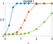
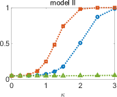
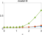
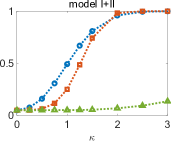
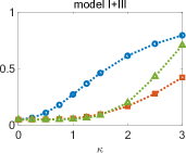
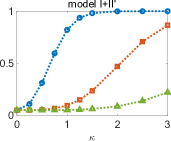
Figure 3.2: Powers of $U^{*[m]}_{N}$ under the mixture models of von Mises distributions.

(blue circle: $m=1$, red square: $m=2$, green triangle: $m=3$)

3.5 Moment generating function

By the series representation (72), the MGF of the limiting GW statistics now have the representations

$$\mathbb{E}\bigl{(}{e^{sU^{[m]}}}\bigr{)}=\prod_{k\geqslant 1}\frac{1}{1-\frac{2s}{\lambda_{k}}}\quad\text{and}\quad\mathbb{E}\bigl{(}{e^{sU^{*[m]}}}\bigr{)}=\mathbb{E}\bigl{(}{e^{sU^{[m]}}}\bigr{)}\prod_{1\leqslant k<m}\Bigl{(}1-\frac{2s}{\lambda_{k}}\Bigr{)},$$ (77)

where $\lambda_{k}:=(2k\pi)^{2m}$. The infinite series represents a meromorphic function in the complex $s$-plane with simple poles at $s=\frac{1}{2}\lambda_{k}$ for $k=1,2,\dots$. Similar to Theorem 2.4, the infinite product in $\mathbb{E}\bigl{(}{e^{sU^{[m]}}}\bigr{)}$ can be simplified.

Theorem 3.4.

For $m\geqslant 1$

$$\mathbb{E}\bigl{(}{e^{sU^{[m]}}}\bigr{)}=\frac{\sqrt{2s}\,e^{\frac{m-1}{2}\pi i}}{2^{m}\prod_{0\leqslant j<m}\sin\bigl{(}{\frac{1}{2}(2s)^{\frac{1}{2m}}e^{\frac{j\pi i}{m}}}\bigr{)}}.$$ (78)

Proof.

The proof is similar to but simpler than that of Theorem 2.4 because the zeros of the polynomial equation $(2\pi z)^{2m}=2s$ have the closed-forms $\zeta_{j}(s)=\frac{1}{2\pi}(2s)^{\frac{1}{2m}}e^{\frac{j\pi i}{m}}$ for $0\leqslant j<2m$. So we first have the finite-product expression

$$\mathbb{E}\bigl{(}{e^{sU^{[m]}}}\bigr{)}=\prod_{0\leqslant j<2m}\Gamma\bigl{(}{1-\zeta_{j}(s)}\bigr{)}.$$

Then we obtain (78) by rearranging the terms by grouping the zeros in pairs and by Euler’s reflection formula. Details are omitted here. ∎

In particular, with $\sigma_{m}:=\frac{1}{2}(2s)^{\frac{1}{2m}}$, we have

$$\mathbb{E}\bigl{(}{e^{sU^{[1]}}}\bigr{)} =\frac{\sigma_{1}}{\sin(\sigma_{1})},$$

$$\mathbb{E}\bigl{(}{e^{sU^{[2]}}}\bigr{)} =\frac{\sigma_{2}^{2}}{\sin(\sigma_{2})\sinh(\sigma_{2})},$$

$$\mathbb{E}\bigl{(}{e^{sU^{[3]}}}\bigr{)} =\frac{2\sigma_{3}^{3}}{\sin(\sigma_{3})\bigl{(}{\cosh(\sqrt{3}\sigma_{3})-\cos(\sigma_{3})}\bigr{)}},$$

$$\mathbb{E}\bigl{(}{e^{sU^{[4]}}}\bigr{)} =\frac{2\sigma_{4}^{4}}{\sin(\sigma_{4})\sinh(\sigma_{4})\bigl{(}{\cosh(\sqrt{2}\sigma_{4})-\cos(\sqrt{2}\sigma_{4})}\bigr{)}}.$$

Since only simple poles instead of branch singularities are involved in the infinite product representation (77) of $\mathbb{E}\bigl{(}{e^{sU^{[m]}}}\bigr{)}$, we can easily invert the MGF by using Laplace transform and obtain the following expressions.

Theorem 3.5.

For $m\geqslant 1$, the density functions $f_{m}(x)$ of $U^{[m]}$ are given by

$$f_{m}(x)=m4^{m}\sum_{k\geqslant 1}\frac{(-1)^{k-1}(k\pi)^{3m-1}e^{\frac{m-1}{2}\pi i}}{\prod_{1\leqslant j<m}\sin\bigl{(}{k\pi e^{\frac{j\pi i}{m}}}\bigr{)}}\,e^{-\frac{1}{2}(2k\pi)^{2m}x},$$

and the distribution functions by

$$1-2m\sum_{k\geqslant 1}\frac{(-1)^{k-1}(k\pi)^{m-1}e^{\frac{m-1}{2}\pi i}}{\prod_{1\leqslant j<m}\sin\bigl{(}{k\pi e^{\frac{j\pi i}{m}}}\bigr{)}}\,e^{-\frac{1}{2}(2k\pi)^{2m}x},$$

for $x>0$.

Proof.

We start with the partial fraction expansion

$$\prod_{k\geqslant 1}\frac{1}{1-\frac{2s}{(2km)^{2m}}}=2m\sum_{k\geqslant 1}\frac{(-1)^{k-1}}{1-\frac{2s}{(2km)^{2m}}}\cdot\frac{(k\pi)^{m-1}e^{\frac{m-1}{2}\pi i}}{\prod_{1\leqslant j<m}\sin\bigl{(}{k\pi e^{\frac{j\pi i}{m}}}\bigr{)}},$$ (79)

which is absolutely convergent for $m\geqslant 2$. This is proved by a standard argument

$$\prod_{k\geqslant 1}\frac{1}{1-\frac{2s}{(2km)^{2m}}}=\sum_{k\geqslant 1}\frac{1}{1-\frac{2s}{(2km)^{2m}}}\prod_{j\neq k}\frac{1}{1-\frac{k^{2m}}{j^{2m}}},$$

where the inner product can be simplified by a similar method of proof used in proving Theorem 3.4

$$\prod_{j\not=k}\frac{1}{1-\frac{k^{2m}}{j^{2m}}}=(-1)^{k-1}\frac{2m(k\pi)^{m-1}e^{\frac{m-1}{2}\pi i}}{\prod_{1\leqslant j<m}\sin\bigl{(}e^{\frac{j\pi i}{m}}k\pi\bigr{)}}\qquad(k\geqslant 1;m\geqslant 2).$$

For large $k$ and $m\geqslant 2$, the terms in (79) decrease in the order

$$2^{m}m(k\pi)^{m-1}\exp\biggl{(}{-k\pi\sum_{1\leqslant j<m}\sin\frac{j\pi}{m}}\biggr{)}=2^{m}m(k\pi)^{m-1}\exp\left(-k\pi\cot\frac{\pi}{2m}\right).$$

Note that $\cot\frac{\pi}{2m}\sim\frac{2m}{\pi}$, we see that the partial fraction expansion (79) converge absolutely and very fast for $m\geqslant 2$.

Thus the decomposition (79) implies that $U^{[m]}$ is an infinite sum of exponential distributions, and the expressions for the density and the distribution functions follow when $m\geqslant 2$, which are also easily checked to hold when $m=1$ (see Watson (1961)). ∎

In particular, the density function of $U^{[1]}$ is given by

$$f_{1}(x)=4\sum_{k\geqslant 1}(-1)^{k-1}(k\pi)^{2}e^{-2(k\pi)^{2}x}\qquad(x>0);$$

as in Watson (1961), and that of $U^{[2]}$ by

$$f_{2}(x)=32\sum_{k\geqslant 1}\frac{(-1)^{k+1}(k\pi)^{5}}{\sinh(k\pi)}\,e^{-8(k\pi)^{4}x}\qquad(x\geqslant 0).$$

4 The generalized Cramér-von Mises statistics

In this section, we examine the corresponding generalized Cramér-von Mises (GCvM) test statistics.

4.1 A new class of GCvM goodness-of-fit statistics

Recall that $F_{N}(x)$ denotes the empirical distribution function of the i.i.d. sequence of random variables $\{X_{1},\ldots,X_{N}\}$. The Cramér-von Mises statistics is defined by

$$\omega_{N}=\int_{0}^{1}\widetilde{B}_{N}(x)^{2}\,\mathrm{d}x,$$

where $\widetilde{B}_{N}(x)=\sqrt{N}(F_{N}(x)-x)=\sqrt{N}\int_{0}^{1}(\mathds{1}_{\{t\leqslant x\}}-x)\,\mathrm{d}F_{N}(t)$ is as before. We generalize the GCvM statistic by defining

$$\omega^{[m]}_{N}=\int_{0}^{1}\widetilde{B}^{[m]}_{N}(x)^{2}\,\mathrm{d}x\qquad(m\geqslant 1),$$

where $\widetilde{B}^{[1]}_{N}(x)=\widetilde{B}_{N}(x)$ and

$$\widetilde{B}^{[m]}_{N}(x)=\begin{cases}\displaystyle\int_{0}^{x}\widetilde{B}^{[m-1]}_{N}(t)\,\mathrm{d}t,&\mbox{if $m$ is odd},\\ \displaystyle\int_{0}^{x}\widetilde{B}^{[m-1]}_{N}(t)\,\mathrm{d}t-\int_{0}^{1}(1-t)\widetilde{B}^{[m-1]}_{N}(t)\,\mathrm{d}t,&\mbox{if $m$ is even}.\end{cases}$$

As we will see in detail later, the correction term $-\int_{0}^{1}(1-t)\widetilde{B}^{[m-1]}_{N}(t)\,\mathrm{d}t$ in the even case has the effect of keeping the template functions invariant in the sense of (81), which induces the invariance of the statistics under the reflection of the data $X_{i}\mapsto 1-X_{i}$.

The iterated empirical measures $\widetilde{B}^{[m]}_{N}(x)$ are also expressible in terms of template functions. Let $b_{m}(y)$ be a normalized Bernoulli polynomial defined in (53).

Lemma 4.1.

For $m\geqslant 1$

$$\widetilde{B}^{[m]}_{N}(x)=\int_{0}^{1}\widetilde{\tau}_{m}(t;x)\,\mathrm{d}F_{N}(t),$$

where

$$\widetilde{\tau}_{m}(t;x) =\frac{(x-t)^{m-1}}{(m-1)!}\mathds{1}_{\{t\leqslant x\}}-2^{m-1}\left(b_{m}\left(\text{\scalebox{0.9}{$\frac{t+x}{2}$}}\right)+(-1)^{m}b_{m}\left(\text{\scalebox{0.9}{$\frac{t-x}{2}$}}\right)\right)$$

$$=(-1)^{m-1}2^{m-1}b_{m}\left(\text{\scalebox{0.9}{$\frac{t-x}{2}$}}+1\right)\mathds{1}_{\{t\leqslant x\}}+(-1)^{m-1}2^{m-1}b_{m}\left(\text{\scalebox{0.9}{$\frac{t-x}{2}$}}\right)\mathds{1}_{\{t>x\}}$$

$$\qquad-2^{m-1}b_{m}\left(\text{\scalebox{0.9}{$\frac{t+x}{2}$}}\right).$$ (80)

Following the same construction of the template functions used in the generalizations of the AD and Watson statistics, we require the template functions to be orthogonal to the eigenfunctions of lower degrees. From the eigenfunction expansion (89) given later, we also propose the truncated version of the template functions

$$\widetilde{\tau}^{*}_{m}(t;x)=\widetilde{\tau}_{m}(t;x)-2\sum_{1\leqslant k<m}\frac{1}{(\pi k)^{m}}\cos\Bigl{(}k\pi x-\text{\scalebox{0.9}{$\frac{m\pi}{2}$}}\Bigr{)}\cos(k\pi t)$$

and define the truncated version of the generalized CvM statistics

$$\omega^{*[m]}_{N}=\int_{0}^{1}\widetilde{B}^{*[m]}_{N}(x)^{2}\,\mathrm{d}x\quad\text{where}\quad\widetilde{B}^{*[m]}_{N}(x)=\int_{0}^{1}\widetilde{\tau}^{*}_{m}(t;x)\,\mathrm{d}F_{N}(x).$$

A graphical rendering of the first four template functions of $\widetilde{\tau}^{*}_{m}(t;x)$ is given in Figure 4.1.

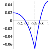
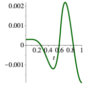
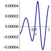
Figure 4.1: Template functions $\widetilde{\tau}^{*}_{m}(\cdot;x_{0})$ for the generalized Cramér-von Mises statistics; here $x_{0}=\frac{\sqrt{5}-1}{2}$, the reciprocal of the golden ratio.

From the definitions, we obtain the following invariance properties.

Lemma 4.2.

The template functions satisfy

$$\widetilde{\tau}_{m}(1-t;1-x)=(-1)^{m}\widetilde{\tau}_{m}(t;x)\quad\text{and}\quad\widetilde{\tau}^{*}_{m}(1-t;1-x)=(-1)^{m}\widetilde{\tau}^{*}_{m}(t;x).$$ (81)

The generalized CvM statistics are invariant under the reflection of the data $X_{i}\mapsto 1-X_{i}$.

Proof of Lemma 4.1.

Write

$$\widetilde{\tau}_{m}(t;x)=\frac{(x-t)^{m-1}}{(m-1)!}\,\mathds{1}_{\{0\leqslant t\leqslant x\}}-g_{m}(t;x),$$

where

$$g_{m}(t;x)=2^{m-1}\left(b_{m}\left(\text{\scalebox{0.9}{$\frac{t+x}{2}$}}\right)+(-1)^{m}b_{m}\left(\text{\scalebox{0.9}{$\frac{t-x}{2}$}}\right)\right).$$

Let $g_{0}(t;x)=x$. Then, $g_{m}(t;x)$ satisfies, for $m\geqslant 2$,

$$\begin{split}g_{m}(t;x)=\begin{cases}\displaystyle\int_{0}^{x}g_{m-1}(t;v)\,\mathrm{d}v,&\mbox{if $m$ is odd},\\ \displaystyle\int_{0}^{x}g_{m-1}(t;v)\,\mathrm{d}v+\frac{(1-t)^{m}}{m!}\\ \displaystyle\qquad-\int_{0}^{1}(1-v)g_{m-1}(t;v)\,\mathrm{d}v,&\mbox{if $m$ is even}.\end{cases}\end{split}$$ (82)

To solve this recurrence relation, we write

$$g_{m}(t;x)=\sum_{0\leqslant k\leqslant m}g_{m,k}(t)x^{k}\qquad(m\geqslant 1).$$

Then we have $g_{1,1}=1$, and

$$g_{m,k}=\frac{g_{m-1,k-1}}{k}=\cdots=\frac{g_{m-k,0}}{k!}\qquad(m\geqslant 2;k\geqslant 0).$$

Thus it suffices to examine the sequence $c_{m}:=g_{m,0}$ in more detail. By (82), we see that $c_{m}=0$ if $m$ is odd, and

$$c_{m}=\frac{(1-t)^{m}}{m!}-\sum_{0\leqslant j<m}\frac{c_{m-1-j}}{(j+2)!}\qquad(m\geqslant 2),$$

if $m$ is even, with $c_{0}:=1$. This sequence is easily solved by considering the generating function $c(z):=\sum_{m\geqslant 0}c_{2m}z^{m}$, which satisfies

$$c(z)=\frac{\sqrt{z}(e^{(2-t)\sqrt{z}}+e^{t\sqrt{z}})}{e^{2\sqrt{z}}-1},$$

and it follows that for even $m\geqslant 0$

$$c_{m}=2^{m-1}\left(b_{m}\Bigl{(}{1-\text{\scalebox{0.9}{$\frac{t}{2}$}}}\Bigr{)}+b_{m}\Bigl{(}{\text{\scalebox{0.9}{$\frac{t}{2}$}}}\Bigr{)}\right).$$

Note that this holds also for odd $m$ for which $c_{m}=0$. By the known relation

$$b_{m}(1-x)=(-1)^{m}b_{m}(x),$$ (83)

we see that $c_{m}=2^{m}\,b_{m}\left(\text{\scalebox{0.9}{$\frac{t}{2}$}}\right)$ when $m$ is even. Consequently,

$$g_{m}(t;x)=\sum_{0\leqslant j\leqslant\left\lfloor m/2\right\rfloor}\frac{2^{2j}x^{m-2j}}{(m-2j)!}\,b_{2j}\left(\text{\scalebox{0.9}{$\frac{t}{2}$}}\right)\qquad(m\geqslant 0).$$

This convolution sum can be simplified as follows.

$$g_{m}(t;x) =[z^{m}]e^{xz}\left(\frac{ze^{tz}}{e^{2z}-1}+\frac{ze^{-tz}}{1-e^{-2z}}\right)$$

$$=[z^{m}]\frac{ze^{xz}\left(e^{tz}+e^{(2-t)z}\right)}{e^{2z}-1}$$

$$=2^{m-1}\left(b_{m}\left(\text{\scalebox{0.9}{$\frac{x+t}{2}$}}\right)+b_{m}\left(1+\text{\scalebox{0.9}{$\frac{x-t}{2}$}}\right)\right)$$

$$=2^{m-1}\left(b_{m}\left(\text{\scalebox{0.9}{$\frac{x+t}{2}$}}\right)+(-1)^{m}b_{m}\left(\text{\scalebox{0.9}{$\frac{t-x}{2}$}}\right)\right),$$ (84)

which completes the proof of the lemma. ∎

4.2 The limiting GCvM processes: KL expansions and covariance kernel

In this section, we examine the limiting distribution of the GCvM statistic under the null hypothesis $H_{0}$. The arguments are almost identical to those used for the GW statistics in Sec. 3.2; thus some details are omitted.

Again the Wiener process on $[0,1]$ and the Brownian bridge are denoted by $W(x)$ and $B(x)$, respectively. Using the template $\widetilde{\tau}_{m}(t;x)$ given in (80), we define the limiting GCvM processes

$$\widetilde{B}^{[m]}(x)=\int_{0}^{1}\widetilde{\tau}_{m}(t;x)\,\mathrm{d}W(t)=\int_{0}^{1}\widetilde{\tau}_{m}(t;x)\,\mathrm{d}B(t),$$

$$\widetilde{B}^{*[m]}(x)=\int_{0}^{1}\widetilde{\tau}^{*}_{m}(t;x)\,\mathrm{d}W(t)=\int_{0}^{1}\widetilde{\tau}^{*}_{m}(t;x)\,\mathrm{d}B(t).$$

Since the Brownian bridge $B(\cdot)$ is of the class $C^{0}$ on $[0,1]$, we have by induction that $\widetilde{B}^{[m]}(\cdot)$ and $\widetilde{B}^{*[m]}(\cdot)$ are of the class $C^{m-1}$ on $[0,1]$.

Lemma 4.3.

Let $\mu$ be any finite measure on $[0,1]$. Then, as $N\to\infty$, $\widetilde{B}^{[m]}_{N}(\cdot)\stackrel{{\scriptstyle d}}{{\to}}\widetilde{B}^{[m]}(\cdot)$ and $\widetilde{B}^{*[m]}_{N}(\cdot)\stackrel{{\scriptstyle d}}{{\to}}\widetilde{B}^{*[m]}(\cdot)$ in $L^{2}([0,1],\mu)$ and in $L^{\infty}([0,1])$, and $\omega^{[m]}_{N}\stackrel{{\scriptstyle d}}{{\to}}\omega^{[m]}$ and $\omega^{*[m]}_{N}\stackrel{{\scriptstyle d}}{{\to}}\omega^{*[m]}$, where

$$\omega^{[m]}=\int_{0}^{1}\widetilde{B}^{[m]}(x)^{2}\,\mathrm{d}x\quad\text{and}\quad\omega^{*[m]}=\int_{0}^{1}\widetilde{B}^{*[m]}(x)^{2}\,\mathrm{d}x.$$

Proof.

The same as that for Lemma 3.2. ∎

We now derive the covariance functions of the continuous centered Gaussian processes $\widetilde{B}^{[m]}(\cdot)$ on $[0,1]$.

Theorem 4.1.

For $m\geqslant 1$

$$\mathrm{Cov}\bigl{(}{\widetilde{B}^{[m]}(x),\widetilde{B}^{[m]}(y)}\bigr{)} =-2^{2m-1}\left(b_{2m}\Bigl{(}{\text{\scalebox{0.9}{$\frac{x+y}{2}$}}}\Bigr{)}+(-1)^{m}b_{2m}\Bigl{(}{\text{\scalebox{0.9}{$\frac{|x-y|}{2}$}}}\Bigr{)}\right)$$

$$=\displaystyle 2\sum_{k\geqslant 1}\frac{\cos\bigl{(}{k\pi x-\frac{1}{2}m\pi}\bigr{)}\cos\bigl{(}{k\pi y-\frac{1}{2}m\pi}\bigr{)}}{(k\pi)^{2m}},$$ (85)

$$\mathrm{Cov}\bigl{(}{\widetilde{B}^{*[m]}(x),\widetilde{B}^{*[m]}(y)}\bigr{)} =\mathrm{Cov}\bigl{(}{\widetilde{B}^{[m]}(x),\widetilde{B}^{[m]}(y)}\bigr{)}$$ (86)

$$\quad-2\sum_{1\leqslant k<m}\frac{\cos\bigl{(}{k\pi x-\frac{1}{2}m\pi}\bigr{)}\cos\bigl{(}{k\pi y-\frac{1}{2}m\pi}\bigr{)}}{(k\pi)^{2m}}.$$

In particular,

$$\mathrm{Var}\bigl{(}{\widetilde{B}^{[m]}(x)}\bigr{)}=-2^{2m-1}\left(b_{2m}(x)+(-1)^{m}b_{2m}(0)\right),$$

$$\mathrm{Var}\bigl{(}{\widetilde{B}^{*[m]}(x)}\bigr{)}=\mathrm{Var}\bigl{(}{\widetilde{B}^{[m]}(x)}\bigr{)}-2\sum_{1\leqslant k<m,\,k:\rm even}\frac{1}{(k\pi)^{2m}}.$$

The covariance functions (85) for $m=1,2$ are given, respectively, by

$$\mathrm{Cov}\bigl{(}{\widetilde{B}^{[1]}(x),\widetilde{B}^{[1]}(y)}\bigr{)} =x\wedge y-xy,$$

$$\mathrm{Cov}\bigl{(}{\widetilde{B}^{[2]}(x),\widetilde{B}^{[2]}(y)}\bigr{)} =\text{\scalebox{0.9}{$\frac{1}{45}$}}-\text{\scalebox{0.9}{$\frac{x^{2}+y^{2}}{6}$}}+\text{\scalebox{0.9}{$\frac{(x\vee y)^{3}+3(x\wedge y)xy}{6}$}}-\text{\scalebox{0.9}{$\frac{x^{4}+6x^{2}y^{2}+y^{4}}{24}$}}.$$

Proof of Theorem 4.1.

The generating function of $g_{m}(t;x)$ in (84) is

$$G(z;t,x)=\sum_{m\geqslant 1}g_{m}(t;x)z^{m-1}=\frac{e^{xz}\left(e^{tz}+e^{(2-t)z}\right)}{e^{2z}-1}-\frac{1}{z},$$ (87)

and

$$H(z;t,x)=\sum_{m\geqslant 1}\widetilde{\tau}_{m}(t;x)z^{m-1}=e^{(x-t)z}\mathds{1}_{\{0\leqslant t\leqslant x\}}-G(z;t,x).$$

Thus the covariance function of $\widetilde{B}^{[m]}(\cdot)$ can be represented as

$$K_{m}(x,y) :=\mathrm{Cov}\bigl{(}{\widetilde{B}^{[m]}(x),\widetilde{B}^{[m]}(y)}\bigr{)}$$

$$=\int_{0}^{1}\widetilde{\tau}_{m}(t;x)\widetilde{\tau}_{m}(t;y)\,\mathrm{d}t=[z^{m-1}w^{m-1}]J(z,w;x,y),$$

where

$$J(z,w;x,y) =\int_{0}^{1}H(z;t,x)H(w;t,y)\,\mathrm{d}t$$

$$=\int_{0}^{x\wedge y}e^{(x-t)z+(y-t)w}\,\mathrm{d}t-\int_{0}^{x}e^{(x-t)z}G(w;t,y)\,\mathrm{d}t$$

$$\quad-\int_{0}^{y}e^{(y-t)w}G(z;t,x)\,\mathrm{d}t+\int_{0}^{1}G(z;t,x)G(w;t,y)\,\mathrm{d}t.$$

Let $\Delta:=x+y$. Straightforward calculations using (87) yield

$$J(z,w;x,y) =\frac{1}{z-w}\left(\frac{e^{w\Delta}}{e^{2w}-1}-\frac{e^{z\Delta}}{e^{2z}-1}\right)-\frac{1}{zw}$$

$$\qquad+\begin{cases}\displaystyle\frac{1}{z+w}\left(\frac{e^{(2-\delta)z}}{e^{2z}-1}+\frac{e^{\delta w}}{e^{2w}-1}\right),&\mbox{if }\delta:=y-x>0,\\ \displaystyle\frac{1}{z+w}\left(\frac{e^{\delta z}}{e^{2z}-1}+\frac{e^{(2-\delta)w}}{e^{2w}-1}\right),&\mbox{if }\delta:=x-y>0.\end{cases}$$

It follows that

$$[z^{m-1}w^{m-1}]\frac{1}{z-w}\left(\frac{e^{w\Delta}}{e^{2w}-1}-\frac{e^{z\Delta}}{e^{2z}-1}\right)-\frac{1}{2zw}$$

$$\qquad=[z^{m-1}w^{m-1}]\sum_{\ell\geqslant 2}b_{\ell}\left(\text{\scalebox{0.9}{$\frac{\Delta}{2}$}}\right)\,2^{\ell-1}\frac{w^{\ell-1}-z^{\ell-1}}{z-w}$$

$$\qquad=-b_{2m}\left(\text{\scalebox{0.9}{$\frac{\Delta}{2}$}}\right)\,2^{2m-1}.$$

Similarly, by (83),

$$[z^{m-1}w^{m-1}]\frac{1}{z+w}\left(\frac{e^{(2-\delta)z}}{e^{2z}-1}+\frac{e^{\delta w}}{e^{2w}-1}\right)-\frac{1}{2zw}$$

$$\qquad=[z^{m-1}w^{m-1}]\sum_{\ell\geqslant 2}b_{\ell}\left(\text{\scalebox{0.9}{$\frac{\delta}{2}$}}\right)\,2^{\ell-1}\frac{w^{\ell-1}-(-z)^{\ell-1}}{z+w}$$

$$\qquad=(-1)^{m-1}b_{2m}\left(\text{\scalebox{0.9}{$\frac{\delta}{2}$}}\right)\,2^{2m-1},$$

when $x<y$. The same expression also holds when $x>y$ provided we replace $\delta$ by $x-y$. Thus in either case

$$K_{m}(x,y)=-2^{2m-1}\left(b_{2m}\left(\text{\scalebox{0.9}{$\frac{x+y}{2}$}}\right)+(-1)^{m}b_{2m}\left(\text{\scalebox{0.9}{$\frac{|x-y|}{2}$}}\right)\right).$$

Note that this identity implies another one by its decomposition

$$\int_{0}^{x\wedge y}\frac{(x-t)^{m-1}(y-u)^{m-1}}{(m-1)!^{2}}\,\mathrm{d}t-\int_{0}^{x}\frac{(x-t)^{m-1}}{(m-1)!}\,g_{m}(t;y)\,\mathrm{d}t$$

$$\qquad-\int_{0}^{y}\frac{(y-t)^{m-1}}{(m-1)!}\,g_{m}(t;x)\,\mathrm{d}t+\int_{0}^{1}g_{m}(t;x)g_{m}(t;y)\,\mathrm{d}t$$

$$=-2^{2m-1}\left(b_{2m}\Bigl{(}{\text{\scalebox{0.9}{$\frac{x+y}{2}$}}}\Bigr{)}+(-1)^{m}b_{2m}\left(\text{\scalebox{0.9}{$\frac{|x-y|}{2}$}}\right)\right).$$ (88)

The proof of (86) relies on the relations

$$\int_{0}^{1}\widetilde{\tau}_{m}(t;x)\cos\Bigl{(}k\pi y-\text{\scalebox{0.9}{$\frac{m\pi}{2}$}}\Bigr{)}\cos(k\pi t)\,\mathrm{d}t=\frac{\cos\bigl{(}k\pi x-\frac{m\pi}{2}\bigr{)}\cos\bigl{(}k\pi y-\frac{m}{2}\pi\bigr{)}}{(k\pi)^{m}}$$

and

$$\begin{split}&\int_{0}^{1}\cos\Bigl{(}k\pi x-\text{\scalebox{0.9}{$\frac{m\pi}{2}$}}\Bigr{)}\cos(k\pi t)\cos\Bigl{(}k\pi y-\text{\scalebox{0.9}{$\frac{m\pi}{2}$}}\Bigr{)}\cos(k\pi t)\,\mathrm{d}t\\ &\qquad=\text{\scalebox{0.9}{$\frac{1}{2}$}}\cos\Bigl{(}k\pi x-\text{\scalebox{0.9}{$\frac{m\pi}{2}$}}\Bigr{)}\cos\Bigl{(}k\pi y-\text{\scalebox{0.9}{$\frac{m\pi}{2}$}}\Bigr{)}.\end{split}$$

The former follows from the same generating function approach used above and the latter is trivial. ∎

Starting from the expansion

$$\widetilde{\tau}_{m}(t;x)=2\sum_{k\geqslant 1}\frac{1}{(\pi k)^{m}}\cos\Bigl{(}k\pi x-\text{\scalebox{0.9}{$\frac{m\pi}{2}$}}\Bigr{)}\cos(k\pi t),$$ (89)

and taking the stochastic integral $\int_{0}^{1}\,\mathrm{d}B(t)$ on both sides, we obtain formally the KL expansion

$$\widetilde{B}^{[m]}(x)=\sqrt{2}\sum_{k\geqslant 1}\frac{\cos(k\pi x-\frac{m\pi}{2})}{(k\pi)^{m}}\,\xi_{k},$$ (90)

where

$$\xi_{k}=\sqrt{2}\int_{0}^{1}\cos(k\pi t)\,\mathrm{d}B(t)\sim N(0,1)\ \ \mbox{i.i.d.}$$ (91)

These expansions hold true, again justified by Mercer’s theorem.

Theorem 4.2.

For $m\geqslant 1$, (90) with $\xi_{j}$ defined by (91) holds uniformly in $x\in[0,1]$ with probability 1, and

$$\omega^{[m]}:=\int_{0}^{1}\widetilde{B}^{[m]}(x)^{2}\,\mathrm{d}x=\sum_{k\geqslant 1}\frac{\xi_{k}^{2}}{(k\pi)^{2m}}$$ (92)

and

$$\omega^{*[m]}:=\int_{0}^{1}\widetilde{B}^{*[m]}(x)^{2}\,\mathrm{d}x=\sum_{k\geqslant m}\frac{\xi_{k}^{2}}{(k\pi)^{2m}}$$ (93)

converges with probability 1.

The proof follows mutatis mutandis that of Theorem 3.2 and is omitted.

4.3 Statistic in terms of samples

We now derive the samples representation of the generalized Cramér-von Mises statistic. Since

$$\omega^{[m]}_{N}=N\int_{0}^{1}\biggl{(}\int_{0}^{1}\widetilde{\tau}_{m}(t;x)\widetilde{\tau}_{m}(u;x)\,\mathrm{d}x\biggr{)}\,\mathrm{d}F_{N}(t)\,\mathrm{d}F_{N}(u),$$

it suffices to evaluate the integral between the large parentheses. The method of proof follows closely that of Theorem 4.1.

Theorem 4.3.

The generalized Cramér-von Mises statistic is expressed in terms of samples $X_{i}$’s as

$$\omega^{[m]}_{N}=\text{\scalebox{0.9}{$\frac{1}{N}$}}\sum_{1\leqslant i,j\leqslant N}(-1)^{m-1}2^{2m-1}\left(b_{2m}\Bigl{(}{\text{\scalebox{0.9}{$\frac{X_{i}+X_{j}}{2}$}}}\Bigr{)}+b_{2m}\Bigl{(}{\text{\scalebox{0.9}{$\frac{|X_{i}-X_{j}|}{2}$}}}\Bigr{)}\right),$$

and

$$\omega^{*[m]}_{N}=\omega^{[m]}_{N}-2\sum_{\begin{subarray}{c}1\leqslant k<m1\leqslant i,j\leqslant N\end{subarray}}\frac{\cos\bigl{(}{k\pi X_{i}-\frac{1}{2}m\pi}\bigr{)}\cos\bigl{(}{k\pi X_{j}-\frac{1}{2}m\pi}\bigr{)}}{(k\pi)^{2m}},$$

where $(2m)!b_{2m}(x)$ denotes the Bernoulli polynomial of order $2m$.

The statistics $\omega^{[m]}_{N}$ for $m=1,2$ are given, respectively, by

$$\omega^{[1]}_{N} =\text{\scalebox{0.9}{$\frac{1}{N}$}}\sum_{1\leqslant i,j\leqslant N}\left(\text{\scalebox{0.9}{$\frac{1}{3}$}}-X_{i}\vee X_{j}+\text{\scalebox{0.9}{$\frac{X_{i}^{2}+X_{j}^{2}}{2}$}}\right),$$

$$\omega^{[2]}_{N} =\text{\scalebox{0.9}{$\frac{1}{N}$}}\sum_{1\leqslant i,j\leqslant N}\left(\text{\scalebox{0.9}{$\frac{1}{45}$}}-\text{\scalebox{0.9}{$\frac{X_{i}^{2}+X_{j}^{2}}{6}$}}+\text{\scalebox{0.9}{$\frac{(X_{i}\vee X_{j})^{3}+3(X_{i}\wedge X_{j})X_{i}X_{j}}{6}$}}\right.$$

$$\hskip 113.81102pt\left.-\text{\scalebox{0.9}{$\frac{X_{i}^{4}+6X_{i}^{2}X_{j}^{2}+X_{j}^{4}}{24}$}}\right).$$

Proof.

We consider the integral

$$K_{m}^{*}(s,t) :=\int_{0}^{1}\widetilde{\tau}_{m}(s;x)\widetilde{\tau}_{m}(t;x)\,\mathrm{d}x$$

$$=\int_{s\vee t}^{1}\frac{(x-s)^{m-1}(x-t)^{m-1}}{(m-1)!^{2}}\,\mathrm{d}x-\int_{s}^{1}\frac{(x-s)^{m-1}}{(m-1)!}\,g_{m}(t;x)\,\mathrm{d}x$$

$$\quad-\int_{t}^{1}\frac{(x-t)^{m-1}}{(m-1)!}\,g_{m}(s;x)\,\mathrm{d}x+\int_{0}^{1}g_{m}(s;x)g_{m}(t;x)\,\mathrm{d}x.$$

We will prove that

$$K_{m}^{*}(s,t)=(-1)^{m-1}2^{2m-1}\left(b_{2m}\left(\text{\scalebox{0.9}{$\frac{s+t}{2}$}}\right)+b_{2m}\Bigl{(}{\text{\scalebox{0.9}{$\frac{|s-t|}{2}$}}}\Bigr{)}\right).$$

By (83) and (84), we have, by exchanging $x$ and $t$,

$$g_{m}(x;t)=2^{m-1}\left(b_{m}\left(\text{\scalebox{0.9}{$\frac{x+t}{2}$}}\right)+(-1)^{m}b_{m}\left(\text{\scalebox{0.9}{$\frac{x-t}{2}$}}\right)\right),$$

and

$$\widetilde{g}_{m}(t;x):=g_{m}(1-t;1-x)=(-1)^{m}2^{m-1}\left(b_{m}\left(\text{\scalebox{0.9}{$\frac{x+t}{2}$}}\right)+b_{m}\left(\text{\scalebox{0.9}{$\frac{x-t}{2}$}}\right)\right).$$

These relations imply particularly that

$$\widetilde{g}_{m}(t;x)=g(x;t)\qquad(m\mbox{ even}).$$ (94)

By the change of variables $x\mapsto 1-x$ and by the definition of $\widetilde{g}_{m}(s;x)$, we see that

$$K_{m}^{*}(1-s,1-t) =\int_{0}^{s\wedge t}\frac{(s-x)^{m-1}(t-x)^{m-1}}{(m-1)!^{2}}\,\mathrm{d}x-\int_{0}^{s}\frac{(s-x)^{m-1}}{(m-1)!}\,\widetilde{g}_{m}(t;x)\,\mathrm{d}x$$

$$\quad-\int_{0}^{t}\frac{(t-x)^{m-1}}{(m-1)!}\,\widetilde{g}_{m}(s;x)\,\mathrm{d}x+\int_{0}^{1}\widetilde{g}_{m}(s;x)\widetilde{g}_{m}(t;x)\,\mathrm{d}x,$$

which leads, by symmetry, (88) and (94), to

$$K_{m}^{*}(1-s,1-t)=K_{m}^{*}(s,t)=K_{m}(s;t)\quad(m\mbox{ even}).$$

We are left with the case when $m$ is odd for which we have

$$\widetilde{g}_{m}(t;x)=g(x;t)+2^{m}\,b_{m}\left(\text{\scalebox{0.9}{$\frac{x+t}{2}$}}\right),$$

so that

$$K_{m}^{*}(1-s,1-t)=K_{m}^{*}(s,t)=K_{m}(s,t)+L_{m}(s,t),$$

where

$$\frac{L_{m}(s,t)}{2} :=2^{m-1}\int_{0}^{s}\text{\scalebox{0.9}{$\frac{(s-x)^{m-1}}{(m-1)!}$}}\,b_{m}\left(\text{\scalebox{0.9}{$\frac{x+t}{2}$}}\right)\,\mathrm{d}x$$

$$\qquad+2^{m-1}\int_{0}^{t}\text{\scalebox{0.9}{$\frac{(t-x)^{m-1}}{(m-1)!}$}}\,b_{m}\left(\text{\scalebox{0.9}{$\frac{x+s}{2}$}}\right)\,\mathrm{d}x$$

$$\qquad+4^{m-1}\int_{0}^{1}b_{m}\left(\text{\scalebox{0.9}{$\frac{x+s}{2}$}}\right)b_{m}\left(\text{\scalebox{0.9}{$\frac{x-t}{2}$}}\right)\,\mathrm{d}x$$

$$\qquad+4^{m-1}\int_{0}^{1}b_{m}\left(\text{\scalebox{0.9}{$\frac{x-s}{2}$}}\right)b_{m}\left(\text{\scalebox{0.9}{$\frac{x+t}{2}$}}\right)\,\mathrm{d}x$$

$$=:L_{m,1}+L_{m,2}+L_{m,3}+L_{m,4}.$$

We will prove that for odd $m$

$$L_{m}(s,t)=2^{2m}\,b_{2m}\left(\text{\scalebox{0.9}{$\frac{s+t}{2}$}}\right).$$

Indeed, this relation holds also for even $m$ but in the form

$$L_{m}(s,t)=(-1)^{m-1}2^{2m}\,b_{2m}\left(\text{\scalebox{0.9}{$\frac{s+t}{2}$}}\right)\quad(m\geqslant 1).$$

We will apply the Fourier series expansion

$$2^{m-1}\,b_{m}(x)=(-1)^{\lceil\frac{m}{2}\rceil}\sum_{j\geqslant 1}\text{\scalebox{0.9}{$\frac{\sin(2j\pi x)}{(j\pi)^{m}}$}}\quad(m\mbox{ odd}).$$ (95)

which holds only for $0\leqslant x\leqslant 1$ (for $0<x<1$ when $m=1$). Thus we cannot simply substitute the Fourier series into the integrals of $L_{m}$. For that purpose, we split first the integrals at $x=t$ and use the relation

$$b_{m}(-x)=-b_{m}(x)-\frac{x^{m-1}}{(m-1)!}\quad(m\mbox{ odd})$$

as follows.

$$L_{m,3} =4^{m-1}\int_{0}^{1}b_{m}\left(\text{\scalebox{0.9}{$\frac{x+s}{2}$}}\right)b_{m}\left(\text{\scalebox{0.9}{$\frac{x-t}{2}$}}\right)\,\mathrm{d}x$$

$$=-4^{m-1}\int_{0}^{t}b_{m}\left(\text{\scalebox{0.9}{$\frac{x+s}{2}$}}\right)b_{m}\left(\text{\scalebox{0.9}{$\frac{t-x}{2}$}}\right)\,\mathrm{d}x$$

$$\quad-\underbrace{2^{m-1}\int_{0}^{t}\frac{(t-x)^{m-1}}{(m-1)!}b_{m}\left(\text{\scalebox{0.9}{$\frac{x+s}{2}$}}\right)\,\mathrm{d}x}_{=L_{m,2}}$$

$$\quad+4^{m-1}\int_{t}^{1}b_{m}\left(\text{\scalebox{0.9}{$\frac{x+s}{2}$}}\right)b_{m}\left(\text{\scalebox{0.9}{$\frac{x-t}{2}$}}\right)\,\mathrm{d}x.$$

Similarly,

$$L_{m,4} =4^{m-1}\int_{0}^{1}b_{m}\left(\text{\scalebox{0.9}{$\frac{x-s}{2}$}}\right)b_{m}\left(\text{\scalebox{0.9}{$\frac{x+t}{2}$}}\right)\,\mathrm{d}x$$

$$=-4^{m-1}\int_{0}^{s}b_{m}\left(\text{\scalebox{0.9}{$\frac{s-x}{2}$}}\right)b_{m}\left(\text{\scalebox{0.9}{$\frac{t+x}{2}$}}\right)\,\mathrm{d}x-L_{m,1}$$

$$\quad+4^{m-1}\int_{s}^{1}b_{m}\left(\text{\scalebox{0.9}{$\frac{x-s}{2}$}}\right)b_{m}\left(\text{\scalebox{0.9}{$\frac{x+t}{2}$}}\right)\,\mathrm{d}x.$$

Thus

$$\frac{L_{m}(s,t)}{2}:= -4^{m-1}\int_{0}^{t}b_{m}\left(\text{\scalebox{0.9}{$\frac{x+s}{2}$}}\right)b_{m}\left(\text{\scalebox{0.9}{$\frac{t-x}{2}$}}\right)\,\mathrm{d}x$$

$$+4^{m-1}\int_{t}^{1}b_{m}\left(\text{\scalebox{0.9}{$\frac{x+s}{2}$}}\right)b_{m}\left(\text{\scalebox{0.9}{$\frac{x-t}{2}$}}\right)\,\mathrm{d}x$$

$$-4^{m-1}\int_{0}^{s}b_{m}\left(\text{\scalebox{0.9}{$\frac{s-x}{2}$}}\right)b_{m}\left(\text{\scalebox{0.9}{$\frac{t+x}{2}$}}\right)\,\mathrm{d}x$$

$$+4^{m-1}\int_{s}^{1}b_{m}\left(\text{\scalebox{0.9}{$\frac{x-s}{2}$}}\right)b_{m}\left(\text{\scalebox{0.9}{$\frac{x+t}{2}$}}\right)\,\mathrm{d}x.$$

All parameters are now inside the unit interval, and we can then apply the Fourier series expansion (95). It follows that

$$\text{\scalebox{0.9}{$\frac{L_{m}(s,t)}{2}$}}:=\sum_{j,\ell\geqslant 1}\text{\scalebox{0.9}{$\frac{I(j,\ell;s,t)}{(j\pi)^{m}(\ell\pi)^{m}}$}},$$

where

$$I(j,\ell;s,t):= -\int_{0}^{t}\sin(j\pi(x+s))\sin(\ell\pi(t-x))\,\mathrm{d}x$$

$$+\int_{t}^{1}\sin(j\pi(x+s))\sin(\ell\pi(x-t))\,\mathrm{d}x$$

$$-\int_{0}^{s}\sin(j\pi(s-x))\sin(\ell\pi(t+x))\,\mathrm{d}x$$

$$+\int_{s}^{1}\sin(j\pi(x-s))\sin(\ell\pi(x+t))\,\mathrm{d}x.$$

It is then straightforward to show that

$$I(j,\ell;s,t)=\begin{cases}0,&\mbox{if }\ell\neq j\\ \cos(j\pi(s+t)),&\mbox{if }\ell=j,\end{cases}$$

implying that

$$L_{m}(s,t)=2\sum_{j\geqslant 1}\text{\scalebox{0.9}{$\frac{\cos(j\pi(s+t))}{(j\pi)^{2m}}$}}=2^{2m}\,b_{2m}\left(\text{\scalebox{0.9}{$\frac{s+t}{2}$}}\right)$$

for odd $m$. ∎

4.4 Power comparisons

We gather here our Monte Carlo simulation results in Figures 4.2–4.4 for the power comparison of the test statistics $\omega_{N}^{*[1]}=\omega_{N}^{[1]}$, $\omega_{N}^{*[2]}$ and $\omega_{N}^{*[3]}$. We adopt the same simulation settings as in the generalized AD statistics in Sec. 2.5. The null hypothesis $H_{0}$ is that $F$ is the normal distribution with zero mean and unit variance; we assume that $N=100$ samples are available. The size of the tests is 0.05, and the critical values are estimated by simulations. We conducted Monte Carlo simulations with 100,000 replications.

We first assume that the true distribution is normal with mean $\mu$ and variance $\sigma^{2}$. The estimated power functions of $\omega_{N}^{*[m]}$ for $m=1,2,3$ are summarized in Figures 4.2 and 4.3.

The pattern of the highest power variations exhibited in Figures 4.2 and 4.3 is almost identical to that of the generalized AD statistics in Figures 2.2 and 2.3, although the generalize AD is slightly superior to the generalized CvM.

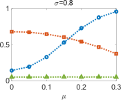
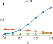
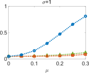
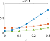
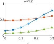
Figure 4.2: Powers of $\omega^{[m]}_{N}$ for $\mu\in[0,0.3]$ and $\sigma\in\{0.8,0.9,1,1.1,1.2\}$.

(blue circle: $m=1$, red square: $m=2$, green triangle: $m=3$)

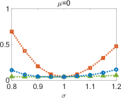
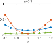
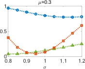
Figure 4.3: Powers of $\omega^{[m]}_{N}$ for $\sigma\in[0.8,1.2]$ and $\mu\in\{0,0.1,0.2,0.3\}$.

(blue circle: $m=1$, red square: $m=2$, green triangle: $m=3$)

In the case of skew-normal distribution alternatives, Figure 4.4 shows the powers of $\omega_{N}^{*[m]}$ for $m=1,2,3$ when the true density is (40). We set the null hypothesis to be the standard normal distribution which corresponds to the case $\xi=0$, $\omega=1$, and $\alpha=0$ in (40). As in the $\alpha=0$ case, the highest power patterns displayed in Figure 4.4 are almost identical to those of the generalized AD statistics in Figure 2.4. Furthermore, there is a tendency that the powers of $\omega_{N}^{*[m]}$ in Figure 4.4 are smaller than those of the corresponding $A_{N}^{*[m]}$ in Figure 2.4.

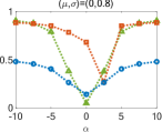
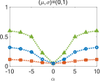
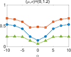
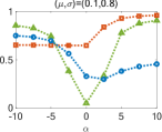
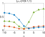
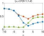
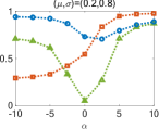
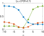
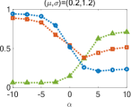
Figure 4.4: Powers of $\omega^{[m]}_{N}$ under skew-normal distributions with index $\alpha$, $\mu\in\{0,0.1,0.2\}$ and $\sigma\in\{0.8,1.0,1.2\}$.

(blue circle: $m=1$, red square: $m=2$, green triangle: $m=3$)

4.5 Moment generating function

The MGF of the limiting GCvM statistics in (92) and (93) have the representations

$$\mathbb{E}\bigl{(}{e^{s\omega^{[m]}}}\bigr{)}=\prod_{k\geqslant 1}\biggl{(}1-\frac{2s}{\lambda_{k}}\biggr{)}^{-\frac{1}{2}}\quad\text{where}\quad\lambda_{k}=(\pi k)^{2m},$$

and

$$\mathbb{E}\bigl{(}{e^{s\omega^{*[m]}}}\bigr{)}=\mathbb{E}\bigl{(}{e^{s\omega^{[m]}}}\bigr{)}\prod_{1\leqslant k<m}\biggl{(}1-\frac{2s}{\lambda_{k}}\biggr{)}^{\frac{1}{2}},$$

which have finite-product expressions as follows.

Theorem 4.4.

For $m\geqslant 1$

$$\mathbb{E}\bigl{(}{e^{s\omega^{[m]}}}\bigr{)}=\sqrt{\frac{\sqrt{2s}\,e^{\frac{m-1}{2}\pi i}}{\prod_{0\leqslant j<m}\sin\bigl{(}{(2s)^{\frac{1}{2m}}e^{\frac{j\pi i}{m}}}\bigr{)}}}.$$

In particular, with $\sigma_{m}:=(2s)^{\frac{1}{2m}}$, we have

$$\mathbb{E}\bigl{(}{e^{s\omega^{[1]}}}\bigr{)} =\sqrt{\frac{\sigma_{1}}{\sin(\sigma_{1})}},$$

$$\mathbb{E}\bigl{(}{e^{s\omega^{[2]}}}\bigr{)} =\sqrt{\frac{\sigma_{2}^{2}}{\sin(\sigma_{2})\sinh(\sigma_{2})}},$$

$$\mathbb{E}\bigl{(}{e^{s\omega^{[3]}}}\bigr{)} =\sqrt{\frac{\sigma_{3}^{3}}{\sin(\sigma_{3})\bigl{(}{\cosh(\sqrt{3}\sigma_{3})-\cos(\sigma_{3})}\bigr{)}}},$$

$$\mathbb{E}\bigl{(}{e^{s\omega^{[4]}}}\bigr{)} =\sqrt{\frac{2\sigma_{4}^{4}}{\sin(\sigma_{4})\sinh(\sigma_{4})\bigl{(}{\cosh(\sqrt{2}\sigma_{4})-\cos(\sqrt{2}\sigma_{4})}\bigr{)}}}.$$

Appendix A Proof of (17): generalized Anderson-Darling statistic in terms of the samples

We prove (17) in this Appendix, which is copied again here for convenience:

$$A_{N}^{[m]}=-\text{\scalebox{0.9}{$\frac{1}{N}$}}\sum_{1\leqslant i,j\leqslant N}R_{m}(a,b)(\log a+\log b)+\text{\scalebox{0.9}{$\frac{1}{N}$}}\sum_{1\leqslant i,j\leqslant N}Q_{m}(a,b),$$

where for simplicity $a=a_{i,j}:=1-X_{i}\wedge X_{j}$ and $b=b_{i,j}:=X_{i}\vee X_{j}$. While the expression we derive for $Q_{m}(a,b)$, based mostly on direct expansion and straightforward simplification, may not be optimal and likely to be further simplified, it is sufficient to prove (17).

For convenience, define

$$f_{m,k}(x):=x^{-m}P_{k}^{(-m)}(x)=\sqrt{2k+1}\sum_{0\leqslant\ell\leqslant k}\frac{(-1)^{k+\ell}(k+\ell)!}{\ell!(k-\ell)!(m+\ell)!}\,x^{\ell}.$$ (96)

Then, by the proof of Lemma 2.2,

$$A_{N}^{[m]}:=\text{\scalebox{0.9}{$\frac{1}{N}$}}\sum_{1\leqslant i,j\leqslant N}\sum_{0\leqslant k,\ell<m}P_{k}(1-a)P_{\ell}(b)I_{k,\ell}(a,b),$$ (97)

where, by (16),

$$I_{k,\ell}(a,b) :=\int_{0}^{1-a}\frac{x^{m}}{(1-x)^{m}}\,f_{m,k}(x)f_{m,\ell}(x)\,\mathrm{d}x$$

$$\quad+(-1)^{m+k}\int_{1-a}^{b}f_{m,k}(1-x)f_{m,\ell}(x)\,\,\mathrm{d}x$$

$$\quad+(-1)^{k+\ell}\int_{b}^{1}\frac{(1-x)^{m}}{x^{m}}f_{m,k}(1-x)f_{m,\ell}(1-x)\,\mathrm{d}x$$

$$=(-1)^{m+k}\int_{1-a}^{b}f_{m,k}(1-x)f_{m,\ell}(x)\,\mathrm{d}x$$

$$\quad+\left(\int_{a}^{1}+(-1)^{k+\ell}\int_{b}^{1}\right)\frac{(1-x)^{m}}{x^{m}}f_{m,k}(1-x)f_{m,\ell}(1-x)\,\,\mathrm{d}x.$$ (98)

Define

$$\phi_{m,k}(x)=\frac{1}{(m-1)!}\int_{0}^{1}(1-x-t)^{m-1}P_{k}(t)\,\mathrm{d}t.$$

We now derive an alternative expression for $I_{k,\ell}(a,b)$ in which the dependence on $a$ and $b$ is explicitly separated.

Lemma A.1.

$$I_{k,\ell}(a,b)= (-1)^{m+k+1}\int_{a}^{1}\frac{\phi_{m,k}(1-x)}{x^{m}}\,f_{m,\ell}(1-x)\,\mathrm{d}x$$ (99)

$$+(-1)^{k+\ell}\int_{b}^{1}\frac{\phi_{m,\ell}(x)}{x^{m}}\,f_{m,k}(1-x)\,\mathrm{d}x$$

$$+(-1)^{m+k}\int_{0}^{1}f_{m,k}(1-x)f_{m,\ell}(x)\,\mathrm{d}x.$$

Proof.

The reason of introducing the additional polynomials $\phi_{m,k}$ is because the relation

$$P_{k}(1-x)=(-1)^{k}P_{k}(x),$$

does not extend directly to $P_{k}^{(-m)}(x)$ for $m\geqslant 0$ but we do have

$$\phi_{m,k}(1-x)=(-1)^{m+k+1}\phi_{m,k}(x).$$

The definition also implies that

$$P_{k}^{(-m)}(1-x)+(-1)^{m+k+1}P_{k}^{(-m)}(x)=(-1)^{m+k+1}\phi_{m,k}(x),$$

which can be readily proved by definition. Here $\phi_{m,k}(x)$ is a polynomial in $x$ of degree $m$. Note that both $P_{k}^{(-m)}(x)$ and $P_{k}^{(-m)}(1-x)$ are of degree $m+k$, which means that the coefficients of $x^{j}$ for $j>m$ on the left-hand side are all cancelled.

With this relation, we have

$$\int_{0}^{1-a}\frac{x^{m}}{(1-x)^{m}}\,f_{m,k}(x)f_{m,\ell}(x)\,\mathrm{d}x$$

$$\qquad=(-1)^{m+k}\left(\int_{0}^{1-a}f_{m,k}(1-x)f_{m,\ell}(x)\,\mathrm{d}x-\int_{0}^{1-a}\frac{\phi_{m,k}(x)}{(1-x)^{m}}\,f_{m,\ell}(x)\,\mathrm{d}x\right).$$

Similarly,

$$(-1)^{k+\ell}\int_{b}^{1}\frac{(1-x)^{m}}{x^{m}}f_{m,k}(1-x)f_{m,\ell}(1-x)\,\mathrm{d}x$$

$$\qquad=(-1)^{m+k}\left(\int_{b}^{1}f_{m,k}(1-x)f_{m,\ell}(x)\,\mathrm{d}x\right.$$

$$\hskip 85.35826pt\left.-(-1)^{m+\ell+1}\int_{b}^{1}\frac{\phi_{m,\ell}(x)}{x^{m}}\,f_{m,k}(1-x)\,\mathrm{d}x\right).$$

These decompositions, coupling with (98), prove (99). ∎

We now examine the contribution to $A_{N}^{[m]}$ (97) of the first integral in (99).

Lemma A.2.

For $m\geqslant 1$

$$\sum_{0\leqslant k,\ell<m}P_{k}(1-a)P_{\ell}(b)\int_{a}^{1}\frac{1}{x^{m}}\,\phi_{m,k}(x)f_{m,\ell}(1-x)\,\mathrm{d}x$$ (100)

$$\quad=-R_{m}(a,b)\log a+\sum_{0\leqslant\ell\leqslant r\leqslant m-1}c_{m,\ell,r}b^{m-1-r}(ab)^{\ell}(1-a-b)^{r-\ell},$$

where $R_{m}(a,b)$ is given in (18) and

$$c_{m,\ell,r}:=\begin{cases}\displaystyle\frac{(-1)^{r}\binom{m-1}{r}\binom{r}{\ell}\binom{m-1+\ell}{r}}{(m-1)!^{2}(m-1-r)},&\text{if }0\leqslant r\leqslant m-2,\\ \qquad&\\ \displaystyle\frac{(-1)^{m-1}\binom{m-1}{\ell}\binom{m-1+\ell}{\ell}\left(H_{m-1}+H_{\ell}-H_{m-1+\ell}\right)}{(m-1)!^{2}},&\text{if }r=m-1.\end{cases}$$

Here $H_{m}:=\sum_{1\leqslant j\leqslant m}j^{-1}$ denotes the harmonic numbers.

By symmetry, we also have the following explicit contribution to $A_{N}^{[m]}$ from the second integral in (99).

Lemma A.3.

For $m\geqslant 1$

$$\int_{b}^{1}\frac{1}{x^{m}}\sum_{0\leqslant k,\ell<m}(-1)^{k+\ell}P_{k}(1-a)P_{\ell}(b)\phi_{m,\ell}(x)f_{m,k}(1-x)\,\mathrm{d}x$$

$$\quad=-R_{m}(a,b)\log b+\sum_{0\leqslant\ell\leqslant r\leqslant m-1}c_{m,\ell,r}a^{m-1-r}(ab)^{\ell}(1-a-b)^{r-\ell}.$$

Proof of Lemma A.2.

Consider first the integral

$$(-1)^{m+k+1}\int_{a}^{1}\frac{\phi_{m,k}(1-x)}{x^{m}}\,f_{m,\ell}(1-x)\,\mathrm{d}x=\int_{a}^{1}\frac{\phi_{m,k}(x)}{x^{m}}\,f_{m,\ell}(1-x)\,\mathrm{d}x.$$

We begin by deriving a more explicit expression for $\phi_{m,k}(x)$ using (8):

$$\frac{\phi_{m,k}(x)}{\sqrt{2k+1}} =\frac{1}{(m-1)!\sqrt{2k+1}}\int_{0}^{1}(1-x-t)^{m-1}P_{k}(t)\,\mathrm{d}t$$

$$=\frac{1}{(m-1)!}\sum_{0\leqslant r<m}\binom{m-1}{r}(-x)^{m-1-r}$$

$$\hskip 71.13188pt\times\sum_{0\leqslant\ell\leqslant k}\binom{k+\ell}{\ell}\binom{k}{\ell}(-1)^{k+\ell}\int_{0}^{1}(1-t)^{r}t^{\ell}\,\mathrm{d}t$$

$$=\frac{1}{(m-1)!}\sum_{0\leqslant r<m}\binom{m-1}{r}(-x)^{m-1-r}$$

$$\hskip 71.13188pt\times\sum_{0\leqslant\ell\leqslant k}\binom{k+\ell}{\ell}\binom{k}{\ell}(-1)^{k+\ell}\frac{\ell!r!}{(r+\ell+1)!}$$

$$=\sum_{0\leqslant r<m}\frac{(-x)^{m-1-r}}{(m-1-r)!}\sum_{0\leqslant\ell\leqslant k}\frac{(k+\ell)!}{\ell!(k-\ell)!(r+\ell+1)!}\,(-1)^{k+\ell}.$$

By the identity

$$\sum_{0\leqslant\ell\leqslant k}\frac{(k+\ell)!(-1)^{k+\ell}}{\ell!(k-\ell)!(r+\ell+1)!}=\frac{(-1)^{k}r!}{(r-k)!(r+k+1)!}\qquad(r\geqslant k),$$

we then obtain

$$\frac{\phi_{m,k}(x)}{\sqrt{2k+1}}=\sum_{k\leqslant r<m}\frac{r!(-1)^{k+m-1-r}}{(m-1-r)!(r-k)!(r+k+1)!}\,x^{m-1-r}.$$

Consider now

$$\sum_{0\leqslant k<m}P_{k}(1-a)\phi_{m,k}(x)$$

$$\quad=(-1)^{m-1}\sum_{0\leqslant k<m}(2k+1)$$

$$\hskip 56.9055pt\times\sum_{0\leqslant r\leqslant k}\sum_{k\leqslant\ell<m}\frac{(k+r)!\ell!(-1)^{r+\ell}(1-a)^{r}x^{m-1-\ell}}{r!r!(k-r)!(m-1-\ell)!(\ell-k)!(\ell+k+1)!}$$

$$\quad=(-1)^{m-1}\sum_{0\leqslant r\leqslant\ell<m}\frac{\ell!(1-a)^{r}x^{m-1-\ell}}{r!r!(m-1-\ell)!}(-1)^{r+\ell}$$

$$\hskip 56.9055pt\times\sum_{r\leqslant k\leqslant\ell}\frac{(2k+1)(k-r)!}{(k-r)!(\ell-k)!(\ell+k+1)!}$$

$$\quad=(-1)^{m-1}\sum_{0\leqslant r\leqslant\ell<m}\frac{\ell!(1-a)^{r}x^{m-1-\ell}}{r!r!(m-1-\ell)!}(-1)^{r+\ell}{\frac{r!}{\ell!(\ell-r)!}}$$

$$\quad=(-1)^{m-1}\sum_{0\leqslant r\leqslant\ell<m}\frac{(1-a)^{r}x^{m-1-\ell}}{r!(m-1-\ell)!(\ell-r)!}(-1)^{r+\ell}$$

$$\quad=(-1)^{m-1}\frac{(x-a)^{m-1}}{(m-1)!}.$$

Now consider the partial sum

$$\sum_{0\leqslant k<m}P_{k}(1-a)f_{m,k}(1-x)$$

$$\quad=\sum_{0\leqslant k<m}(2k+1)\sum_{0\leqslant r_{1},r_{2}\leqslant k}\frac{(-1)^{r_{1}+r_{2}}(k+r_{1})!(k+r_{2})!(1-a)^{r_{1}}(1-x)^{r_{2}}}{r_{1}!r_{1}!(k-r_{1})!r_{2}!(m+r_{2})!(k-r_{2})!}$$

$$\quad=\sum_{0\leqslant r_{1},r_{2}<m}\frac{(-1)^{r_{1}+r_{2}}(1-a)^{r_{1}}(1-x)^{r_{2}}}{r_{1}!r_{1}!r_{2}!(m+r_{2})!}{\sum_{0\leqslant k<m}(2k+1)\frac{(k+r_{1})!(k+r_{2})!}{(k-r_{1})!(k-r_{2})!}}$$

$$\quad=\sum_{0\leqslant r_{1},r_{2}<m}\frac{(-1)^{r_{1}+r_{2}}(1-a)^{r_{1}}(1-x)^{r_{2}}}{r_{1}!r_{1}!r_{2}!(m+r_{2})!}\cdot{\frac{(m+r_{1})!(m+r_{2})!}{(r_{1}+r_{2}+1)(m-1-r_{1})!(m-1-r_{2})!}}$$

$$\quad=\sum_{0\leqslant r_{1}<m}\frac{(-1)^{r_{1}}(m+r_{1})!(1-a)^{r_{1}}}{r_{1}!r_{1}!(m-1-r_{1})!}\sum_{0\leqslant r_{2}<m}\frac{(-1)^{r_{2}}(1-x)^{r_{2}}}{r_{2}!(r_{1}+r_{2}+1)(m-1-r_{2})!},$$

where we used the same identity (30) as above. Observe that

$$\sum_{0\leqslant r_{2}<m}\frac{(-1)^{r_{2}}(1-x)^{r_{2}}}{r_{2}!(r_{1}+r_{2}+1)(m-1-r_{2})!}$$

$$\qquad=\frac{1}{(m-1)!}\int_{0}^{1}u^{r_{1}}\left(1-(1-x)u\right)^{m-1}\,\mathrm{d}u$$

$$\qquad=\frac{1}{(m-1)!}\sum_{0\leqslant r_{2}<m}\binom{m-1}{r_{2}}x^{r_{2}}\int_{0}^{1}(1-u)^{m-1-r_{2}}u^{r_{1}+r_{2}}\,\mathrm{d}u$$

$$\qquad=\frac{1}{(m-1)!}\sum_{0\leqslant r_{2}<m}\binom{m-1}{r_{2}}\frac{(m-1-r_{2})!(r_{1}+r_{2})!}{(m+r_{1})!}\,x^{r_{2}}$$

$$\qquad=\sum_{0\leqslant r_{2}<m}\frac{(r_{1}+r_{2})!}{r_{2}!(m+r_{1})!}\,x^{r_{2}}.$$

It follows that

$$\sum_{0\leqslant k<m}P_{k}(1-a)f_{m,k}(1-x)$$ (101)

$$\qquad=\frac{1}{(m-1)!}\sum_{0\leqslant r_{2}<m}x^{r_{2}}\sum_{0\leqslant r_{1}<m}\binom{r_{1}+r_{2}}{r_{1}}\binom{m-1}{r_{1}}(-1)^{r_{1}}(1-a)^{r_{1}}.$$

In a similar way,

$$\sum_{0\leqslant\ell<m}P_{\ell}(b)f_{m,\ell}(1-x)$$ (102)

$$\qquad=\frac{1}{(m-1)!}\sum_{0\leqslant\ell_{2}<m}x^{\ell_{2}}\sum_{0\leqslant\ell_{1}<m}\binom{\ell_{1}+\ell_{2}}{\ell_{1}}\binom{m-1}{\ell_{1}}(-1)^{\ell_{1}}b^{\ell_{1}}.$$

Consequently,

$$\int_{a}^{1}\frac{1}{x^{m}}\sum_{0\leqslant k,\ell<m}P_{k}(1-a)P_{\ell}(b)\phi_{m,k}(x)f_{m,\ell}(1-x)\,\mathrm{d}x$$

$$\quad=\frac{(-1)^{m-1}}{(m-1)!^{2}}\int_{a}^{1}\frac{(x-a)^{m-1}}{x^{m}}\sum_{0\leqslant k,\ell<m}\binom{k+\ell}{\ell}\binom{m-1}{k}(-1)^{k}b^{k}x^{\ell}\,\mathrm{d}x$$

$$\quad=\frac{(-1)^{m-1}}{(m-1)!^{2}}\int_{a}^{1}\frac{(x-a)^{m-1}}{x^{m}}[z^{0}]\sum_{0\leqslant k,\ell<m}z^{-\ell}(1-z)^{-k-1}\binom{m-1}{k}(-1)^{k}b^{k}x^{\ell}\,\mathrm{d}x$$

$$\quad=\frac{(-1)^{m-1}}{(m-1)!^{2}}[z^{m-1}]\frac{(1-b-z)^{m-1}}{(1-z)^{m}}\int_{a}^{1}\frac{(x-a)^{m-1}}{x-z}\,\mathrm{d}x$$

$$\quad=\frac{1}{(m-1)!^{2}}[z^{m-1}]\frac{(1-b-z)^{m-1}}{(1-z)^{m}}$$

$$\qquad\qquad\times\sum_{0\leqslant\ell<m}\binom{m-1}{\ell}(-1)^{\ell}(a-z)^{m-1-\ell}\int_{a}^{1}(x-z)^{\ell-1}\,\mathrm{d}x$$

$$\quad=\frac{1}{(m-1)!^{2}}[z^{m-1}]\frac{(1-b-z)^{m-1}}{(1-z)^{m}}\left((a-z)^{m-1}\log\frac{1-z}{a-z}\right.$$

$$\qquad\left.+\sum_{1\leqslant\ell<m}\binom{m-1}{\ell}\frac{(-1)^{\ell}}{\ell}\left((1-z)^{\ell}(a-z)^{m-1-\ell}-(a-z)^{m-1}\right)\right)$$

$$\quad=\frac{1}{(m-1)!^{2}}[z^{m-1}]\Biggl{\{}\frac{(1-b-z)^{m-1}(a-z)^{m-1}}{(1-z)^{m}}\left(\log\frac{1-z}{1-\frac{z}{a}}-\log a\right)$$

$$\hskip 113.81102pt+\sum_{1\leqslant\ell<m}\binom{m-1}{\ell}\frac{(-1)^{\ell}}{\ell}\cdot\frac{(1-b-z)^{m-1}(a-z)^{m-1-\ell}}{(1-z)^{m-\ell}}$$

$$\hskip 113.81102pt-\frac{(1-b-z)^{m-1}(a-z)^{m-1}}{(1-z)^{m}}\sum_{1\leqslant\ell<m}\binom{m-1}{\ell}\frac{(-1)^{\ell}}{\ell}\Biggr{\}}.$$

Note that, by the change of variables $z\mapsto-au/(1-a-u)$, we obtain

$$[z^{m-1}]\frac{(1-b-z)^{m-1}(a-z)^{m-1}}{(1-z)^{m}}$$

$$\qquad=(-1)^{m-1}[u^{m-1}]\frac{((1-a-b)(1-u)+ab)^{m-1}}{(1-u)^{m}}$$

$$\qquad=(-1)^{m-1}[u^{m-1}]\frac{((1-a-b)u+ab)^{m-1}}{(1-u)^{m}}$$

$$\qquad=(-1)^{m-1}\sum_{0\leqslant\ell<m}\binom{m-1}{\ell}(ab)^{\ell}(1-a-b)^{m-1-\ell}[u^{\ell}](1-u)^{-m}$$

$$\qquad=(-1)^{m-1}\sum_{0\leqslant\ell<m}\binom{m-1}{\ell}\binom{m-1+\ell}{\ell}(ab)^{\ell}(1-a-b)^{m-1-\ell}.$$

Similarly,

$$[z^{m-1}]\frac{(1-b-z)^{m-1}(a-z)^{m-1}}{(1-z)^{m}}\log\frac{1-z}{1-\frac{z}{a}}$$

$$\quad=(-1)^{m}\sum_{0\leqslant\ell<m}\binom{m-1}{\ell}\binom{m-1+\ell}{\ell}(ab)^{\ell}(1-a-b)^{m-1-\ell}\left(H_{m-1+\ell}-H_{\ell}\right).$$

Also

$$\sum_{1\leqslant\ell<m}\binom{m-1}{\ell}\frac{(-1)^{\ell}}{\ell}=-H_{m-1}.$$

This proves (100). ∎

We now examine the partial sum involving last integral in (99).

$$\sum_{0\leqslant k,\ell<m}(-1)^{m+k}P_{k}(1-a)P_{\ell}(b)\int_{0}^{1}f_{m,k}(1-x)f_{m,\ell}(x)\,\mathrm{d}x.$$

By (8) and (96), this is already a polynomial in $a$ of degree $m-1$ and in $b$ of degree $m-1$. We can derive a more precise but cumbersome expression for the coefficients.

Lemma A.4.

$$\sum_{0\leqslant k,\ell<m}(-1)^{m+k}P_{k}(1-a)P_{\ell}(b)\int_{0}^{1}f_{m,k}(1-x)f_{m,\ell}(x)\,\mathrm{d}x=\sum_{0\leqslant k,\ell<m}d_{m,k,\ell}a^{k}b^{\ell},$$

where

$$d_{m,k,\ell}:=(-1)^{m+k+\ell}\frac{(k+\ell)!(H_{m+\ell}-H_{\ell})+\displaystyle\sum_{\begin{subarray}{c}0\leqslant r<m\\ r\neq\ell\end{subarray}}\frac{(k+r)!}{\ell-r}\left(\frac{(m+\ell)!}{(m+r)!}-\frac{\ell!}{r!}\right)}{k!^{2}\ell!^{2}(m-1-k)!(m-1-\ell)!}.$$

Proof.

We use the two expansions (101) and (102), and obtain

$$\sum_{0\leqslant k,\ell<m}(-1)^{m+k}P_{k}(1-a)P_{\ell}(b)f_{m,k}(1-x)f_{m,\ell}(x)$$

$$\quad=(-1)^{m}\sum_{0\leqslant k,\ell<m}P_{k}(a)P_{\ell}(b)f_{m,k}(1-x)f_{m,\ell}(x)$$

$$\quad=\frac{(-1)^{m}}{(m-1)!^{2}}\sum_{\begin{subarray}{c}0\leqslant k_{2},\ell_{2}<m\\ 0\leqslant k_{1},\ell_{1}<m\end{subarray}}\binom{k_{1}+k_{2}}{k_{1}}\binom{\ell_{1}+\ell_{2}}{\ell_{1}}\binom{m-1}{k_{1}}\binom{m-1}{\ell_{1}}$$

$$\hskip 142.26378pt\times(-1)^{k_{1}+\ell_{1}}a^{k_{1}}b^{\ell_{1}}x^{k_{2}}(1-x)^{\ell_{2}}$$

$$\quad=(-1)^{m}\sum_{0\leqslant k_{1},k_{2},\ell_{1},\ell_{2}<m}\frac{(k_{1}+k_{2})!(\ell_{1}+\ell_{2})!(-1)^{k_{1}+\ell_{1}}a^{k_{1}}b^{\ell_{1}}}{k_{1}!k_{1}!k_{2}!\ell_{1}!\ell_{1}!\ell_{2}!(m—1-k_{1})!(m-1-\ell_{1})!}\,x^{k_{2}}(1-x)^{\ell_{2}}.$$

Thus

$$\sum_{0\leqslant k,\ell<m}(-1)^{m+k}P_{k}(1-a)P_{\ell}(b)\int_{0}^{1}f_{m,k}(1-x)f_{m,\ell}(x)\,\mathrm{d}x$$

$$\quad=(-1)^{m}\sum_{0\leqslant k_{1},k_{2},\ell_{1},\ell_{2}<m}\frac{(k_{1}+k_{2})!(\ell_{1}+\ell_{2})!(-1)^{k_{1}+\ell_{1}}a^{k_{1}}b^{\ell_{1}}}{k_{1}!k_{1}!\ell_{1}!\ell_{1}!(m-1-k_{1})!(m-1-\ell_{1})!(k_{2}+\ell_{2}+1)!}$$

$$\quad=(-1)^{m}\sum_{0\leqslant k_{1},\ell_{1}<m}\frac{(-1)^{k_{1}+\ell_{1}}a^{k_{1}}b^{\ell_{1}}}{k_{1}!k_{1}!\ell_{1}!\ell_{1}!(m-1-k_{1})!(m-1-\ell_{1})!}$$

$$\hskip 85.35826pt\times\sum_{0\leqslant k_{2},\ell_{2}<m}\frac{(k_{1}+k_{2})!(\ell_{1}+\ell_{2})!}{(k_{2}+\ell_{2}+1)!}.$$

Now

$$\sum_{0\leqslant\ell_{2}<m}\frac{(k_{1}+k_{2})!(\ell_{1}+\ell_{2})!}{(k_{2}+\ell_{2}+1)!}=\begin{cases}\displaystyle\frac{(k_{1}+k_{2})!}{\ell_{1}-k_{2}}\left(\frac{(m+\ell_{1})!}{(m+k_{2})!}-\frac{\ell_{1}!}{k_{2}!}\right),&\mbox{if }k_{2}\neq\ell_{1},\\ (k_{1}+k_{2})!(H_{m+\ell_{1}}-H_{\ell_{1}}),&\mbox{if }k_{2}=\ell_{1}.\end{cases}$$

This proves (A.4). ∎

[Acknowledgments] The authors thank Yoichi Nishiyama for his helpful comments, and Chihiro Hirotsu for bringing the authors’ attention to change-point analysis.

References

- Abramowitz and Stegun (1964) {bbook}[author] \bauthor\bsnmAbramowitz, \bfnmMilton\binitsM. and \bauthor\bsnmStegun, \bfnmIrene A.\binitsI. A. (\byear1964). \btitleHandbook of mathematical functions with formulas, graphs, and mathematical tables. \bseriesNational Bureau of Standards Applied Mathematics Series. \bpublisherU.S. Government Printing Office, Washington, D.C. \bmrnumber0167642 \endbibitem
- Adler (1990) {bbook}[author] \bauthor\bsnmAdler, \bfnmRobert J.\binitsR. J. (\byear1990). \btitleAn introduction to continuity, extrema, and related topics for general Gaussian processes. \bpublisherInstitute of Mathematical Statistics, Hayward, CA. \bmrnumber1088478 \endbibitem