Correlation decoupling of Casimir interaction in an electrolyte driven by external electric fields

Abstract

It has been established for a long time that the long range van der Waals or thermal Casimir interaction between two semi-infinite dielectrics separated by a distance $H$ is screened by an intervening electrolyte. Here we show how this interaction is modified when an electric field of strength $E$ is applied parallel to the dielectric boundaries, leading to a non-equilibrium steady state with a current. The presence of the field induces a long range thermal repulsive interaction, scaling just like the thermal Casimir interaction between dielectrics without the intervening electrolyte, i.e. as $1/H^{3}$. At small $E$ the effect is of order $E^{2}$ while at large fields it saturates to an $E$ independent value. We explain the results in terms of a decoupling mechanism between the charge density fluctuations of cations and anions at large applied fields.

Introduction– Fluctuation induced interactions are ubiquitous both from the fundamental as well as applied point of view and can arise due to both quantum and thermal fluctuations par05 ; woo16 ; dan23 . These interactions can be varied by changing material properties in the case of van der Waals interactions woo16 or by chemical variations of surface properties in the case of the critical Casimir effect RevModPhys.90.045001 . Another way to modify these interactions is to apply external fields, for example electric or magnetic fields dea16 ; mah21 . The application of an electric field generates a current in systems which can conduct, and the presence of a current implies that the system is out of equilibrium. The out of equilibrium nature of the problem means that standard equilibrium methods, for example the Lifshitz formulation of van der Waals forces cannot be applied directly Advances , it can however be extended to compute van der Waals forces between dielectrics held at different temperatures Antezza2 ; Antezza1 ; Kardar . Out of equilibrium thermal or classical fluctuation induced forces can be studied via the Langevin dynamics of dipole fields in dielectrics and/or ionic Brownian dynamics in electrolytes UOELangevin ; UOELiving ; BSLu .

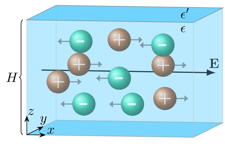
Figure 1: Geometry of the confined electrolyte of dielectric constant $\epsilon$ between two dielectric semispaces of dielectric constant $\epsilon^{\prime}$, driven by an external electric filed ${\bf E}$. $H$ is the separation between the dielectrics, $z$ is the normal coordinate with the bottom surface located at $z=0$.

An illuminating model in the theory of the thermal Casimir effect is the living conductor model where two plates containing an electrolyte interact across a dielectric gap jan04 ; UOELiving ; YLevin . In equilibrium this model exhibits the universal long range attractive Casimir interaction for free scalar field theories Advances . Recently dea16 , it was shown that when an electric field is applied parallel to one plate this attractive Casimir interaction is reduced by the fact that the driving electric field destroys or scrambles the charge-charge correlations which yield the attraction in the equilibrium case. More recently mah21 , the force between two planar dielectrics with an electrolyte in between, and driven by an electric field has been studied as a function of the field strength (see the schematic in Fig. (1)). Here, it was found that driving the system leads to an effective long range interaction which can be attractive or repulsive. This is a particularly interesting result as, in equilibrium, the long range van der Waals interaction between two dielectric slabs with an intervening electrolyte is established to be screened, i.e., it decays exponentially with the plate separation at distances larger than the Debye screening length nin76 ; net01 . The Casimir interaction in the presence of a driving electrostatic field was analyzed by using an approximation scheme for the linearized stochastic density functional theory (SDFT) that describes the classical charge fluctuations in the system mah21 . This leads to an effective theory reminiscent of statistical field theories where the introduction of anisotropy (due to the applied field) is mismatched with the thermal noise and leads to long-range correlations gar90 ; gri90 which in turn generate a long-range fluctuation induced interaction Sengers1 ; Sengers2 . It furthermore leads to a limiting result at small driving electric field magnitude $E$, with the force scaling as $E^{4}$, while at large fields it scales as $E^{2}$. These results are somewhat surprising, first one might expect that the small field force should scale as $E^{2}$ unless there is some fine tuning arising naturally in the problem, secondly it is not clear how a laterally imposed large electric field could lead to arbitrarily large forces.

Here we reconsider the problem studied in Ref. mah21 in the limit where the dielectric constant of the surrounding (outer) dielectrics, $\epsilon^{\prime}$, is much smaller than the dielectric constant of the intervening solvent, $\epsilon$. This case can be solved without any approximation beyond the linearization of the SDFT for the electrolyte. We find that an electric field does indeed induce a long range interaction and this interaction gives a total, or net, repulsive force per unit area

$$f_{\rm t}(H)=\frac{\zeta(3)}{8\pi\beta H^{3}}\left[1-\left({1+\frac{\beta^{2}q^{2}E^{2}}{m^{2}}}\right)^{-{\textstyle\frac{1}{2}}}\right].$$ (1)

as well as exponentially screened terms which are thus subdominant for large $H$. In Eq. (1) $\beta=1/(k_{\mathrm{B}}T)$ where $k_{\mathrm{B}}$ is Boltzmann’s constant and $T$ is the temperature of the system (assumed constant), $\pm q$ is the charge of the cations/anions, and $m=\sqrt{2\overline{\rho}q^{2}/(\epsilon k_{\mathrm{B}}T)}$ is the inverse Debye screening length where $\overline{\rho}$ is the mean density of cations/anions. We thus predict that the long range force in this dielectric set up is always repulsive, scales as $E^{2}$ for small applied electric fields and saturates for large applied fields. We also identify the origin of this limiting form of the repulsion at large electric fields which is due to the decoupling of the cationic and anionic charge fluctuations, which then become independent of one another for large fields. For $E=0$, we recover the well known result for the screened thermal Casimir interaction nin76 ; net01 , from our purely dynamical approach.

The model– We consider (see Fig. (1)) two semi-infinite dielectrics of dielectric constant $\epsilon^{\prime}$ separated by a slab of thickness $H$ in the direction $z$, containing an electrolyte solution of dielectric constant $\epsilon$ and ionic densities $\overline{\rho}$ of cations and anions of charges $\pm q$, but with otherwise identical properties, notably they have the same friction coefficient $\gamma$. These conditions of symmetry can be relaxed but the resulting formulas become much more complicated. This symmetric case is sufficient to highlight the underlying physics of the problem. The over-damped Langevin equation for the anions and cations (labeled by the index $i$) is given by

$$\gamma\frac{\mathrm{d}{\bf x}_{i}}{\mathrm{d}t}=q_{i}({\bf E}-\nabla\phi({\bf x}_{i}))+\sqrt{2k_{\mathrm{B}}T\gamma}~{}\bm{\eta}_{i}(t),$$ (2)

which corresponds to force balance between the frictional force on the left hand side and the electrical and thermal noise forces on the right hand side. The first term on the right is the force due to the applied electric field parallel to the slabs (taken to be in the direction $x$) ${\bf E}=E{\bf e}_{x}$, and the second one is the force due to the electric field generated by the ions themselves:

$$\phi({\bf x})=q\int\mathrm{d}{\bf x}^{\prime}G({\bf x},{\bf x}^{\prime})[\rho_{+}({\bf x}^{\prime})-\rho_{-}({\bf x}^{\prime})].$$ (3)

In Eq. (3) $\rho_{\pm}({\bf x})=\sum_{i\pm}\delta({\bf x}-{\bf x}_{i})$ denotes the density of ions/cations and $G({\bf x},{\bf x}^{\prime})$ is the Green’s function for the slab geometry where

$$\nabla\cdot\epsilon({\bf x})\nabla G({\bf x},{\bf x}^{\prime})=-\delta({\bf x}-{\bf x}^{\prime}).$$ (4)

Finally, the term $\bm{\eta}_{i}(t)$ denotes a Gaussian white noise of zero mean with $\langle\eta_{i\alpha}(t)\eta_{j\beta}(t^{\prime})\rangle=\delta_{ij}\delta_{\alpha\beta}\delta(t-t^{\prime})$, where $\alpha$ and $\beta$ label the spatial components $(x,\,y,\,z)$. Starting from the Langevin equations we can formally write down the SDFT for the densities $\rho_{\pm}({\bf x})$, this non-linear theory becomes solvable if we expand about a background of constant density $\rho_{\pm}({\bf x})=\overline{\rho}+n_{\pm}({\bf x})$. Note that when the electric field is parallel to the bounding surfaces it does not generate a surface charge and so the expansion of the density about its average bulk value is justified. The analysis of the linearized SDFT is simplified by using the fluctuations of the total density $n_{\mathrm{t}}({\bf x})=n_{+}({\bf x})+n_{-}({\bf x})$ and the fluctuations of the charge density $\rho_{\mathrm{c}}({\bf x})=q[n_{+}({\bf x})-n_{-}({\bf x})]=qn_{\mathrm{d}}({\bf x})$. One thus finds SM

$$\frac{\partial n_{\mathrm{t}}({\bf x})}{\partial t} = \nabla\cdot D[\nabla n_{\mathrm{t}}({\bf x})-\beta qn_{\mathrm{d}}({\bf x}){\bf E}]+\xi_{\mathrm{t}}({\bf x},t),$$ (5)

$$\frac{\partial n_{\mathrm{d}}({\bf x})}{\partial t} = \nabla\cdot D[\nabla n_{\mathrm{d}}({\bf x})-\beta qn_{\mathrm{t}}({\bf x}){\bf E}+2q\beta\overline{\rho}\nabla\phi({\bf x})]$$ (6)

$$+\xi_{\mathrm{d}}({\bf x},t).$$

where the spatio-temporal white noise terms are independent and have correlation functions $\langle\xi_{\mu}({\bf x},t)\xi_{\nu}({\bf x}^{\prime},t^{\prime})\rangle=-4\overline{\rho}D\delta_{\mu\nu}\delta(t-t^{\prime})\nabla^{2}\delta({\bf x}-{\bf x}^{\prime}),\,\mu,\nu\in\{\mathrm{t},\mathrm{d}\}$. The term $D$ is the diffusion constant of the cations and anions, given by $D=k_{\mathrm{B}}T/\gamma$. The boundary conditions on the linearized SDFT are no-flux boundary conditions, so $\nabla_{z}n_{\mathrm{t}}({\bf x})=0$ and $\nabla_{z}n_{\mathrm{d}}({\bf x})+2q\beta\overline{\rho}\nabla_{z}\phi({\bf x})=0$ at the boundaries $z=0$ and $z=H$. No flux boundary conditions are also imposed independently on the noise terms, as the noise is independent of the ionic distribution at the time when it acts. The second boundary condition (on $n_{\mathrm{d}}({\bf x})$) is non-local due to the appearance of the electrostatic potential which depends on the whole charge density in the problem. This non-locality can be dealt with Future , but here we consider the simplifying case where we assume that $\epsilon^{\prime}\ll\epsilon$. This means that both the density and the electrostatic potential have the same, Neumann boundary conditions at the bounding surfaces. Consequently, both fields, $n_{\mathrm{t}}({\bf x})$ and $n_{\mathrm{d}}({\bf x})$, as well as the noise fields, can be expanded in terms of a Fourier cosine expansion SM , yielding

$$n_{\mu}({\bf x}_{\|},z,t) = \int\frac{\mathrm{d}{\bf k}}{(2\pi)^{2}}\sum_{n=0}^{\infty}\frac{1}{\sqrt{N_{n}}}\tilde{n}_{\mu n}({\bf k},t)\exp(\mathrm{i}{\bf k}\cdot{\bf x}_{\|})\cos(p_{n}z),\,\mu\in\{\mathrm{t},\mathrm{d}\},$$ (7)

where $p_{n}=n\pi/H$ enforces the Neumann conditions at $z=0$ and $z=H$, while $N_{n}$ normalizes the corresponding eigenfunction, with $N_{n}=H/2$ for $n\geq 1$ and $N_{0}=H$. The Fourier transform is taken in the plane $\mathbf{x}_{\|}=(x,y)$ parallel the bounding dielectric surfaces. In the steady state the resulting Lyapunov equation SM can be solved analytically for the equal time correlation functions $\langle\tilde{n}_{\mu m}({\bf k},t)\tilde{n}_{\nu n}(({\bf k}^{\prime},t)\rangle=(2\pi)^{2}\delta_{mn}\delta({\bf k}+{\bf k^{\prime}})\tilde{C}_{\mu\nu n}$, $\mu,\nu\in\{\mathrm{t},\mathrm{d}\}$, where

$$\tilde{C}_{\mathrm{tt}n}({\bf k}) = 2\overline{\rho}\frac{(k^{2}+p_{n}^{2})\left[(K^{2}+p_{n}^{2})(K^{2}+k^{2}+2p_{n}^{2})+2\beta^{2}q^{2}E^{2}k_{x}^{2}\right]}{(K^{2}+k^{2}+2p_{n}^{2})\left[(K^{2}+p_{n}^{2})(k^{2}+p_{n}^{2})+\beta^{2}q^{2}E^{2}k_{x}^{2}\right]},$$ (8a)

$$\tilde{C}_{\mathrm{td}n}({\bf k}) = -\tilde{C}_{\mathrm{dt}n}({\bf k})=\mathrm{i}2\overline{\rho}\frac{\beta qEk_{x}m^{2}(k^{2}+p_{n}^{2})}{(K^{2}+k^{2}+2p_{n}^{2})\left[(K^{2}+p_{n}^{2})(k^{2}+p_{n}^{2})+\beta^{2}q^{2}E^{2}k_{x}^{2}\right]},$$ (8b)

$$\tilde{C}_{\mathrm{dd}n}({\bf k}) = 2\overline{\rho}\frac{(k^{2}+p_{n}^{2})\left[(k^{2}+p_{n}^{2})(K^{2}+k^{2}+2p_{n}^{2})+2\beta^{2}q^{2}E^{2}k_{x}^{2}\right]}{(K^{2}+k^{2}+2p_{n}^{2})\left[(K^{2}+p_{n}^{2})(k^{2}+p_{n}^{2})+\beta^{2}q^{2}E^{2}k_{x}^{2}\right]}$$ (8c)

with $K^{2}=k^{2}+m^{2}$ and $k_{x}={\bf e}_{x}\cdot{\bf k}$.

We now turn to the computation of the force between the two dielectrics. In writing Eq. (4) we have implicitly assumed that the dipole degrees of freedom in the system adjust instantaneously to generate image charges, and are thus fully equilibrated with respect to a given configuration of charge density (dynamics of dipoles being governed by rapid electronic degrees of freedom orders of magnitude faster than the diffusive dynamics of the ions of the electrolyte). However, in principle, potentially slower dynamics of the dipoles in the dielectrics can be taken into account UOELangevin . The dipole fluctuations also generate their own thermal component of the Casimir force between two dielectrics, which would be present in the absence of any electrolyte, i.e., when $\overline{\rho}=0$. There is also an ideal gas component coming from the ions when they are uncharged or due to the constant non-fluctuating part of the densities which is by definition also assumed to be equilibrated. This means that the average total force per unit area is given by

$$f_{\rm t}=f_{\rm vdW}+f_{\rm ion}+2\,\overline{\rho}\,k_{\mathrm{B}}T,$$ (9)

where $f_{\rm vdW}$ is the van der Waals interaction between the two dielectrics in the absence of ions (including contributions from the zero and non-zero Matsubara frequencies), which are assumed to be instantaneously equilibrated, and $2\,\overline{\rho}\,k_{\mathrm{B}}T$ is the bulk ideal van’t Hoff pressure term, which is also assumed to be equilibrated as it is not affected by the external field, and will be ignored subsequently since it is independent of separation $H$. The second term $f_{\rm ion}$ is the contribution due to the ions which can be deduced by constructing a stress tensor from the local body force, which can then be written down in terms of the density fluctuations, and is given by SM ; kru18

$$\sigma_{\alpha\beta}({\bf x})= -\frac{k_{\mathrm{B}}T}{4\,\overline{\rho}}\delta_{\alpha\beta}(n^{2}_{\mathrm{t}}({\bf x})+n^{2}_{\mathrm{d}}({\bf x}))+$$ (10)

$$\epsilon({\bf x})(\nabla_{\alpha}\phi({\bf x})\nabla_{\beta}\phi({\bf x})-\frac{1}{2}\delta_{\alpha\beta}[\nabla\phi({\bf x})]^{2}).$$

The first term on the right hand side is generated by the density fluctuations, while the second term is the contribution from the standard Maxwell stress tensor. Furthermore, in the limit $\epsilon^{\prime}\ll\epsilon$ only the part of the stress tensor inside the electrolyte slab yields a non-zero contribution to the force.

The outward acting surface force density due to the ions at $z=0$ is given by $f_{\rm ion}=-\sum_{\beta}\langle\sigma_{z\,\beta}(0,0,0^{+})-\sigma_{z\,\beta}(0,0,0^{-})\rangle$ (by translational invariance in the $(x,y)$ plane). The average is taken over the spatio-temporal noise, the minus sign comes from the downward normal and $z=0^{\pm}$ denotes the position just above and just below the bounding surface at $z=0$, respectively. In the limit $\epsilon^{\prime}\ll\epsilon$ the stress tensor is diagonal and we find

$$f_{\rm ion}=\frac{k_{\mathrm{B}}T}{4\overline{\rho}}\langle n^{2}_{\mathrm{t}}({\bf 0})+n^{2}_{\mathrm{d}}({\bf 0})\rangle+\frac{\epsilon}{2}\langle\nabla_{\|}\phi({\bf 0})\rangle^{2},$$ (11)

where $\nabla_{\|}$ denotes the gradient in the $(x,y)$ plane. One can explicitly extract the terms which give the total $H$ dependent force (including the contribution from the dielectric slabs $f_{\rm vdW}$ in Eq. (9)) SM , these are

$$f_{\rm t}(H)=-\frac{1}{\beta}\int\frac{\mathrm{d}{\bf k}}{(2\pi)^{2}}\sum_{n}\frac{1}{2N_{n}}\frac{K^{2}(k^{2}+p_{n}^{2})^{2}(K^{2}+k^{2}+2p_{n}^{2})+\beta^{2}q^{2}E^{2}k_{x}^{2}\left[2k^{2}(k^{2}+p_{n}^{2})+m^{2}(k^{2}+2p_{n}^{2})\right]}{(k^{2}+p_{n}^{2})(K^{2}+k^{2}+2p_{n}^{2})\left[(k^{2}+p_{n}^{2})(K^{2}+p_{n}^{2})+\beta^{2}q^{2}E^{2}k_{x}^{2}\right]}.$$ (12)

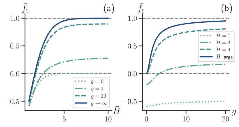
Figure 2: Dependence of the interaction force $\bar{f}_{\mathrm{t}}=f_{\mathrm{t}}/[\zeta(3)/8\pi\beta H^{3}]$ on (a) the separation $\bar{H}=Hm$ with fixed coupling constant $g=\beta qE/m$ and (b) $g$ with fixed $\bar{H}$. The asymptotic large $\bar{H}$ and $g$ results are shown as the dashed lines $\bar{f}_{\mathrm{t}}=1$.

For $E=0$, the above equation yields the well known equilibrium result for the screened thermal Casimir interaction which can be written in the same limit $\epsilon^{\prime}\ll\epsilon$ as nin76

$$f_{\rm t}(H) = -\frac{1}{4\pi\beta H^{3}}\int_{mH}^{\infty}\mathrm{d}K\,K^{2}\left(\coth K-1\right)$$ (13)

which is rather remarkable viewed in the context of the formalism adopted here. The charge fluctuations of the electrolyte obviously produce a repulsive thermal Casimir interaction which cancels exactly the attractive thermal Casimir interaction between the two bounding dielectrics. This effect was already pointed out explicitly for an equilibrium system in jan04 and was also discussed previously by a number of other authors att87 ; att88 . In the $E=0$ limiting case this attractive interaction is

$$f_{\rm vdW}(H)=-\frac{\zeta(3)}{8\pi\beta H^{3}}.$$ (14)

The residual interaction after this cancellation then turns out to be attractive and screened.

The integral and sum in Eq. (12) can be evaluated analytically SM but the result is rather unwieldy and does not have an intuitive interpretation. However, the large distance behavior of the interaction, more precisely in the limit where $Hm\gg 1$, can be simply extracted from the small $k$ and $p_{n}$ components in Eq. (12). This then gives for large $H$ the particularly simple formula in Eq. (1) for the dominant large distance component of $f_{\rm t}(H)$, which is exact up to terms which decay as $\exp(-2mH)$. We emphasize that the long distance repulsion is only present for non zero $E$ and is a purely non-equilibrium effect. For small $E$ the force behaves as $f_{\rm t}(H)=\frac{\zeta(3)}{16\pi\beta H^{3}}\frac{\beta^{2}E^{2}q^{2}}{m^{2}}$. On the other hand, for strong electric field driving as $E\to\infty$ in the same limit of $\epsilon^{\prime}\ll\epsilon$, we find

$$f_{\rm t}(H)\!=\!\frac{\zeta(3)}{8\pi\beta H^{3}}-\frac{2}{4\pi\beta H^{3}}\!\!\int_{\frac{mH}{\sqrt{2}}}^{\infty}\!\!\mathrm{d}KK^{2}\!\left(\coth K-1\right).$$ (15)

The first term is a repulsive thermal Casimir force of exactly the same absolute magnitude as the equilibrium attraction between two dielectrics with no intervening electrolyte. This result can be understood as a correlation decoupling between the cations and anions due to the strong external electric field SM , indicated by Eq. (8b). If only the cationic type was present then the effect of the electric field would be to drive all the cations at the same average velocity $v=\beta DqE$. In the rest frame of the cations the system would then be in an effective equilibrium. Charge fluctuations in this equilibrium state would then generate a repulsive thermal Casimir interaction as given by Eq. (15). However, the same argument is equally valid for the anions that move with velocity $v=-\beta DqE$. The crucial point is that due to the external electrostatic field driving the dynamics of the cations and anions becomes decoupled in the limit of $E\to\infty$, and so they both generate a repulsive force of the form in Eq. (15), subtracting off the attractive thermal Casimir interaction of the dielectrics then giving the net repulsive force Eq. (15). Notice that the $E$ dependence in the decouplimg effect occurs via a coupling constant $g=\beta Eq/m$ which can be written as $g=v/v^{*}$, where $v^{*}=Dm$ is an intrinsic velocity scale for the non-driven electrolyte system, corresponding exactly to the same non-equilibrium parameter found in Ref. dea16 for the Casimir interaction between two plates containing Brownian electrolytes, where one is driven by an electric field.

The second term in Eq. (15), which again exhibits a form of the screened thermal Casimir force, is also consistent with the above interpretation in terms of the correlation decoupling SM . In fact the inverse screening length of $m/\sqrt{2}$ indicates that the ions of either type are screening independently. Since in the rest frame of the anions/cations they are in an effective equilibrium at half the total density (see above), the Casimir interaction is exactly twice (explicit factor 2 in the second term of Eq. (15)) the screened Casimir force at $m/\sqrt{2}$ screening length, giving the strong electric field driving limiting law a consistent intuitive interpretation.

One can express the full interaction $f_{\rm t}$ at arbitrary separation $H$ and external electric field strength $E$ in terms of integrals which need to be evaluated numerically. In Fig. (2) we have shown $f_{\rm t}$ as functions of $\bar{H}=Hm$ (i.e. with $H$ measured in units of the Debye length) and $g$, where $f_{t}$ are normalized by the absolute value of van der Waals attraction in Eq. (14). In Fig. (2a) we see the behavior of $f_{\rm t}$ at fixed values of $g$ as $\bar{H}$ is varied. The lowest curve corresponds to $g=0$ the screened thermal Casimir force given in Eq. (13) which is always attractive. The cases $g=1,\ 10$ and $g\to\infty$ are also shown, at short distances all these forces are attractive but on increasing $\bar{H}$ they become repulsive, the crossover value of $\bar{H}$ from attraction to repulsion decreases on increasing $g$. The large $g$ limits agree with the asymptotic result Eq. (15). In Fig (2b) we show $f_{\rm{t}}$ at fixed values of $\bar{H}$ as a function of $g$. At all separations increasing $g$ increases the repulsive component of the force, at short distances the force remains net attractive but at large distances it eventually becomes net repulsive. The large $\bar{H}$ limits agree with the asymptotic result Eq. (1). $f_{t}$ saturates to the repulsion $\zeta(3)/(8\pi\beta H^{3})$ at either large separation $H$ or large coupling $g$.

Conclusions– Using non-equilibrium SDFT for an electrolyte confined between two dielectrics in an external driving electric field, we first of all recover the well known result for the screened thermal Casimir interaction from a purely dynamical approach. For asymptotically large separations we find a quadratic scaling of the repulsive Casimir interaction for small electric fields, and show that for large electric field it saturates. The exponentially screened terms correspond to the standard screened thermal Casimir force with the Debye screening length for vanishing electric field, and to a Debye screening length at half the ion density for large electric fields, this effect being due to decoupled ionic correlations in the presence of strong external driving. The non-equilibrium effects predicted here could be tested either in the surface force apparatus ric20 or colloidal probe atomic force microscopy interaction geometry Trefalt20 .

Acknowledgments– G.D., B.M. and R.P. acknowledge funding from the Key Project No. 12034019 of the National Natural Science Foundation of China and the support by the Fundamental Research Funds for the Central Universities (Grant No. E2EG0204). D.S.D. acknowledges support from the grant No. ANR-23-CE30-0020-01 EDIPS, and by the European Union through the European Research Council by the EMet-Brown (ERC-CoG-101039103) grant.

References

- (1) L.M. Woods, D.A.R. Dalvit, A. Tkatchenko, P. Rodriguez-Lopez, A.W. Rodriguez and R. Podgornik, Materials perspective on Casimir and van der Waals interactions, Rev. Mod. Phys. 88, 045003 (2016).
- (2) D.M. Dantchev and S. Dietrich, Critical Casimir Effect: Exact Results, Physics Reports, 1005, 1 (2023).
- (3) V.A. Parsegian, Van der Waals Forces: A Handbook for Biologists, Chemists, Engineers, and Physicists, Cambridge University Press (Cambridge) (2005).
- (4) A. Maciołek and S. Dietrich, Collective behavior of colloids due to critical Casimir interactions, Rev. Mod. Phys., 90, 045001 (2018).
- (5) D. S. Dean, B.-S. Lu, A. C. Maggs, and R. Podgornik, Nonequilibrium Tuning of the Thermal Casimir Effect, Phys. Rev. Lett. 116, 240602 (2016).
- (6) S. Mahdisoltani and R. Golestanian, Long-Range Fluctuation-Induced Forces in Driven Electrolytes, Phys. Rev. Lett. 126, 158002 (2021).
- (7) M. Bordag, G. L. Klimchitskaya, U. Mohideen, and V. M. Mostepanenko, Advances in the Casimir Effect (Oxford University Press, New York, 2009).
- (8) M. Antezza, L.P. Pitaevskii, S. Stringari, V.B. Svetovoy, Casimir-Lifshitz force out of thermal equilibrium and asymptotic nonadditivity, PRL 97, 223203 (2006).
- (9) M. Antezza, L. P. Pitaevskii, S. Stringari, and V. B. Svetovoy, Casimir-Lifshitz force out of thermal equilibrium, Phys. Rev. A 77, 022901 (2008).
- (10) M. Krüger, T. Emig, and M. Kardar, Nonequilibrium Electromagnetic Fluctuations: Heat Transfer and Interactions, Phys. Rev. Lett. 106, 210404 (2011).
- (11) D. S. Dean, V. Démery, V. A. Parsegian, and R. Podgornik, Out-of-equilibrium relaxation of the thermal Casimir effect in a model polarizable material, Phys. Rev. E 85, 031108 (2012).
- (12) D. S. Dean and R. Podgornik, Relaxation of the thermal Casimir force between net neutral plates containing Brownian charges, Phys. Rev. E 89, 032117 (2014).
- (13) B.-S. Lu, D. S. Dean and R. Podgornik, Out of equilibrium thermal Casimir effect between Brownian conducting plates, EPL, 112, 20001, (2015).
- (14) B.W. Ninham and J. Mahanty, Dispersion forces, London Academic Press (1976).
- (15) R.R. Netz, Static van der Waals interactions in electrolytes, Eur. Phys. J. E 5, 189 (2001).
- (16) P. L. Garrido, J. L. Lebowitz, C. Maes, and H. Spohn, Long-range correlations for conservative dynamics, Phys. Rev. A 42, 1954 (1990).
- (17) G. Grinstein, D.-H. Lee, and S. Sachdev, Conservation Laws, Anisotropy, and Self-Organized Criticality in Noisy Non- equilibrium Systems, Phys. Rev. Lett. 64, 1927 (1990).
- (18) T. R. Kirkpatrick, J. M. Ortiz de Zárate, and J. V. Sengers, Giant Casimir Effect in Fluids in Nonequilibrium Steady States, PRL 110, 235902 (2013).
- (19) T. R. Kirkpatrick, J. M. Ortiz de Zárate, and J. V. Sengers, Fluctuation-induced pressures in fluids in thermal nonequilibrium steady states, Phys. Rev. E 89, 022145 (2014).
- (20) See Supplementary Material for more detailed explanation of the calculation.
- (21) Guangle Du, D.S. Dean, Bing Miao, R. Podgornik, in preparation.
- (22) M. Krüger, A. Solon, V. Démery, C. M. Rohwer, and D. S. Dean, Stresses in non-equilibrium fluids: Exact formulation and coarse-grained theory, J. Chem. Phys. 148, 084503 (2018).
- (23) V. Démery and D. S. Dean, The conductivity of strong electrolytes from stochastic density functional theory, J. Stat. Mech. 023106 (2016).
- (24) D. S. Dean, Langevin equation for the density of a system of interacting Langevin processes, J. Phys. A 29, L613 (1996).
- (25) B. Jancovici and L. Šamaj, Screening of classical Casimir forces by electrolytes in semi-infinite geometries, J. Stat. Mech. P08006 (2004).
- (26) P. Attard, R. Kjellander and D. J. Mitchell, Interactions between electroneutral surfaces nearing mobile charges, Chem. Phys. Lett. 139, 219 (1987).
- (27) P. Attard, D. J. Mitchell, and B. W. Ninham, Beyond Poisson–Boltzmann: Images and correlations in the electric double layer. I. Counterions only, J. Chem. Phys. 88, 4987 (1988).
- (28) D.S. Dean and R.R. Horgan, Electrostatic fluctuations in soap films, Phys. Rev. E 65, 061603 (2002).
- (29) I.M. Telles, Y. Levin, A. dos Santos, Reversal of Electroosmotic Flow in Charged Nanopores with Multivalent Electrolyte, Langmuir 38, 3817-3823,(2022).
- (30) L. Richter, P. J. Żuk, P. Szymczak, J. Paczesny, K. M. Bkak, T. Szymborski, P. Garstecki, H. A. Stone, R. Hołyst, and C.Drummond, Ions in an AC Electric Field: Strong Long- Range Repulsion Between Oppositely Charged Surfaces, Phys. Rev. Lett. 125, 056001 (2020).
- (31) A. Smith, M. Borkovec, G. Trefalt, Forces between solid surfaces in aqueous electrolyte solutions, Advances in Colloid and Interface Science, 275, 102078 (2020).