Prelimit Coupling and Steady-State Convergence of Constant-stepsize Nonsmooth Contractive SA
Abstract
Motivated by Q-learning, we study nonsmooth contractive stochastic approximation (SA) with constant stepsize. We focus on two important classes of dynamics: 1) nonsmooth contractive SA with additive noise, and 2) synchronous and asynchronous Q-learning, which features both additive and multiplicative noise. For both dynamics, we establish weak convergence of the iterates to a stationary limit distribution in Wasserstein distance. Furthermore, we propose a prelimit coupling technique for establishing steady-state convergence and characterize the limit of the stationary distribution as the stepsize goes to zero. Using this result, we derive that the asymptotic bias of nonsmooth SA is proportional to the square root of the stepsize, which stands in sharp contrast to smooth SA. This bias characterization allows for the use of Richardson-Romberg extrapolation for bias reduction in nonsmooth SA.
1 Introduction
Stochastic Approximation (SA) is a fundamental algorithmic paradigm for solving fixed-point problems iteratively based on noisy observations. SA procedures have been widely used in many application domains, including reinforcement learning (RL), stochastic control and optimization [3, 48, 33, 38]. A typical SA algorithm is of the form
| (1) |
where represent the noise sequence and is a constant stepsize. The SA procedure (1) aims to approximately find the solution to the fixed-point equation where is the expectation of the operator with respect to the noise. Equation (1) covers many popular algorithms, such as the prevalent stochastic gradient descent (SGD) algorithm for minimizing an objective function [34], and variants of TD-learning algorithms for policy evaluation in RL [48].
In this work, we focus on nonsmooth contractive SA, where the operator may be nondifferentiable (in its first argument) and is a contractive mapping with respect to a norm . One prominent example of nonsmooth contractive SA is the celebrated Q-learning algorithm for optimal control in RL [56], where corresponds to the noisy optimal Bellman operator involving a max function. Other common nonsmooth mappings include the largest eigenvalue of a matrix, -norm regularized functions, and their composition with smooth functions [47, 49]. It is of fundamental interest to gain a complete understanding of the evolution and long-run behavior of the iterates generated by nonsmooth contractive SA.
Under suitable conditions on the operator and the noise sequence , the SA iterates form a time-homogeneous Markov chain and quickly converge to some limit random variable [14, 59]. Recent work has developed a suite of results for smooth SA [14, 29, 16], including the geometric convergence of the chain, finite-time bounds on the higher moments, as well as properties of the limit It has been observed that often , due to the use of constant stepsize. The difference is referred to as the asymptotic bias. In particular, for SA with differentiable dynamic, the work [14, 29] makes use of Taylor expansion of to establish that the asymptotic bias is proportional to the stepsize (up to a higher order term), i.e.,
| (2) |
where is some vector independent of and denotes a term that decays faster than . Such a fine-grained characterization of SA iterates gives rise to variance and bias reduction techniques that lead to improved estimation of the target solution , as well as efficient statistical inference procedures [14, 29, 28].
For nonsmooth SA, far little is known. Existing analysis based on the linearization / Taylor expansion of is no longer applicable. Hence, distributional convergence and bias characterization results like (2) have not been established for nonsmooth SA procedures like Q learning. In fact, it is not even clear whether equation (2) remains valid for nonsmooth SA, and if not, what is the correct characterization.
Our Contributions: To investigate the above questions, we consider two important classes of nonsmooth contractive SA algorithms:
- 1.
-
2.
A general form of Q-learning dynamics, which are nonsmooth SA with both additive and multiplicative noise. The model covers both synchronous Q-learning and asynchronous Q-learning as special cases. See Section 3 for the formal description of the model.
The first main result of the paper establishes the weak convergence of the Markov chain to a unique stationary distribution in — the Wasserstein distance of order 2 with respect to the contraction norm — for both the additive noise setting and Q-learning. Moreover, we characterize the geometric convergence rate. As a by-product of our analysis, we derive finite-time upper bounds on , the -th moments of the estimation errors, generalizing the mean-square error (MSE) bound (i.e. ) in [10, 11] to higher moments and the smooth SA results in [14, 51] to nonsmooth SA.
We next turn to the characterization of the stationary distribution of As existing techniques, which are based on linearizing as , are not applicable for nonsmooth SA, we take an alternative approach by studying the limiting behavior of the properly rescaled iterates as the constant stepsize approaches 0. Since the MSE of is of order [10], the proper choice of scaling is by , the diffusion scaling. In particular, we consider the centered and -scaled iterates so that the MSE of is . The weak convergence of to a limit implies that converges weakly to the limit as . Therefore, to understand the stationary distribution and its scaled version , we are interested in characterizing steady-state convergence, i.e., the convergence of as and the limit (if exists). This limit is illustrated by the red solid path in Fig. 1.
As we argue in Section 1.1, existing approaches to steady-state convergence face severe challenges in the nonsmooth SA setting. In this work, we develop a new prelimit coupling technique, which allows us to establish the weak convergence of in to a unique limiting random variable as . Importantly, our technique can handle both additive noise and multiplicative noise, and provide an explicit rate of convergence. An overview of our technique is provided in Section 1.2. We remark that our technique can be potentially applied to the study of steady-state convergence in other stochastic dynamical systems and hence may be of its own interest.
Since convergence in implies convergence of the first two moments of , we obtain the following characterization of the asymptotic bias of the SA iterates:
| (3) |
We further provide a fine-grained characterization of the expectation , which appears above in (3), and relate it to the structure of the SA update (1). Our results show that precisely when the operator is truly nonsmooth, in which case the asymptotic bias is of order . This result stands in sharp contrast to the -order bias of smooth SA in equation (2).
Finally, we explore the implications of the above results for iterate averaging and extrapolation. In particular, we consider applying Polyak-Ruppert (PR) tail averaging [46, 43, 32] and Richardson-Romberg (RR) extrapolation [30] to the iterates generated by contractive SA algorithms. We investigate the resulting estimation errors and biases in the presence of nonsmoothness. In particular, thanks to the bias characterization in (3), we can employ the RR extrapolation technique to eliminate the leading term and reduce the asymptotic bias to a higher order of .
1.1 Challenges of Applying Existing Techniques to Nonsmooth SA
Steady-state convergence, i.e., showing in Figure 1, is a problem of fundamental interest in stochastic dynamical systems, such as queueing networks [27]. One well-known approach to proving steady-state convergence in queueing networks is via justifying the interchange of limits, i.e., equivalence of the solid and dashed paths in Figure 1 [27, 26, 60, 61]. Doing so is well recognized to be technically challenging, often requiring sophisticated “hydro-dynamic limits” methodology [7] as well as a well-defined stochastic differential equation (SDE) with a stationary distribution. In our setting, it is unclear whether nonsmooth SA is associated with such an SDE, let alone the validity of interchanging the limits.
An alternative approach to the steady-state convergence is based on the Basic Adjoint Relationship (BAR) for the generator of the stochastic process. By using BAR with an exponential test function, one may be able to prove convergence of the moment generating function and in turn weak convergence of the corresponding random variables [1, 2, 9]. In our setting, however, the BAR of moment generating functions does not always lead to a straightforward solution. In fact, even for smooth SA dynamics with only additive noise (i.e., ), steady-state convergence is proved in the work [9] only when the limit random variable is Gaussian and under the assumption that the following equation from BAR has a unique solution in :
| (4) |
Verifying this assumption is challenging in general; in [9] this is done only when or under some restricted conditions when . This difficulty is only exacerbated in the broader nonsmooth contractive SA setting, which covers the smooth SA setting considered in [9].
The -scaling in our problem suggests a potential connection to the Langevin diffusion SDE and the literature on the Unadjusted Langevin Algorithm (ULA) [18, 19]. ULA corresponds to the Euler-Maruyama discretization of the Langevin diffusion and is given by
where is a potential function and are i.i.d. Gaussian noise. However, by comparing ULA with the SA update (1) scaled by , one sees that the latter reduces to ULA only when the noise is additive and Gaussian and is a gradient field and positive homogeneous at .
We complement the above discussion with a simple example of nonsmooth contractive SA:
| (5) |
where and . The above dynamic is a special case of (1) with , which is nondifferentiable at . Despite its apparent simplicity, this example already demonstrates some of the complexity in understanding the steady-state behavior of nonsmooth SA. For example, it is unclear how to follow the BAR approach to obtain a functional equation like (4) for the limit . The derivation of (4) in [9] relies on the continuous differentiability of the contraction operator .222In particular, for deriving the limit of the term in [9, Page 15]. Also, incidentally, when , the dynamic (5) becomes an ULA update. The results in [18, 19] on ULA suggest that the limit is not Gaussian as its density function involves a non-quadratic . This contrasts to smooth SA, for which the BAR approach shows that is Gaussian [9]. As we soon see, the techniques in this paper bypass the need of working directly with and imposing assumptions on equations like (4).
1.2 Prelimit Coupling Technique
To overcome the challenges discussed in the previous subsection, we develop a prelimit coupling technique that can be used to establish the desired steady-state convergence without restrictive assumptions. We establish this result by proving convergence in Wasserstein distance , i.e.,
for a random variable , where denotes the distribution of . Our approach applies coupling arguments to the prelimit random variables with and consists of three steps.
Step 1: Gaussian Noise and Rational Stepsize
First, we assume that the noise sequence is i.i.d. Gaussian. Consider two stepsizes and , where . We have the corresponding scaled iterates and generated by equation (1). The main idea is to couple these two sequences in such a way that one step of corresponds to steps of :
Note that and are identically distributed under the Gaussian noise assumption. Under this coupling, we establish convergence of the squared distance under some appropriate norm . Sending to infinity gives Generalizing this argument to rational stepsizes and , we conclude that is a Cauchy sequence with respect to . Consequently, there exists a limit such that
Step 2: General Stepsize
Still assuming Gaussian noise, we prove that is continuous in with respect to . To this end, we consider two real-valued stepsizes and and couple the sequences and , this time by letting them share the same noise:
We again control the squared distance , and then set followed by , thus establishing the continuity property Since is dense in , together with the result from step 1, we obtain
Step 3: General Noise
In this step, we relax the Gaussian noise assumption. Suppose the sequence is driven by some general noise , and let be driven by Gaussian noise with matching first two moments. Setting , we use a multivariate Berry-Esseen bound in Wasserstein distance [6] to show that there exists a coupling between and such that
Under this noise coupling, we bound , which in turn bounds , thereby establishing that and have the same distributional limit as .
Following the above three-step procedure, the majority of the technical work goes into obtaining tight estimates for squared distances of the form , with potentially mismatched stepsizes and time indices . Doing so under the nonsmooth SA dynamics requires carefully analyzing the multi-step dynamics and leveraging the contractive property via a generalized Moreau envelope argument.
1.3 Notations
We use to denote an open ball centering at with radius with respect to -norm. A function is if it is times continuously differentiable. An operator is said to be -contractive w.r.t. the norm if for some ,
| (6) |
A function is called -smooth w.r.t. some norm if , where is the dual norm of
Let denote the space of square-integrable distributions on . For a random vector , let denote the distribution of and its covariance matrix. The Wasserstein 2-distance between two distributions and in is defined as
where is the set of joint distributions in with marginal distributions and .
For a finite set , we use to denote the probability simplex over . Given , we denote by the multinomial distribution with event probabilities and number of trials .
For two real valued functions , we write if , and we write if there exist such that . We say that is superpolynomial if
Paper organization.
The remainder of the paper is organized as follows. In Section 2 we present the model and the main results for SA with additive noise. In Section 3 we extend these results to Q-learning. In Section 4 we explore the implications of our results for Polyak-Ruppert averaging and Richardson-Romberg extrapolation. We outline the proofs of our main results in Section 5. We provide numerical experiments that corroborate our theoretical results in Section 6. We discuss additional related work in Section 7.
2 Nonsmooth Stochastic Approximation with Additive Noise
In this section, we consider contractive nonsmooth stochastic approximation with additive noise.
2.1 Model Setup
We consider the following stochastic approximation iteration with additive noise:
| (7) |
where is an operator, is a constant stepsize and is a sequence of i.i.d zero-mean noise.
Stochastic approximation subsumes many important iterative algorithms. For example, if for some function that is twice continuously differentiable, -smooth and -strongly convex, then the update (7) corresponds to Stochastic Gradient Descent (SGD) for minimizing [34]. If where is a Hurwitz matrix, then (7) becomes Linear SA, which in turn covers the TD-learning algorithm in reinforcement learning [29, 51]. In both examples, the operator is at least -smooth and contractive in (or its weighted version).
In this work, we consider a more general class of SA algorithms with a potentially nonsmooth operator . We only assume that is contractive with respect to an arbitrary norm.
Assumption 1 (Contractive ).
The operator is -contractive for some with respect to some norm .
By Banach fixed point theorem, the fixed point equation has a unique solution .
We consider the following moment assumption for the additive noise , indexed by .
Assumption 2 ().
The random variables have finite -th moments.
2.2 Moments Bounds and Convergence to Stationary Distribution
We first derive finite-time upper bounds on , the -th moments of the estimation errors, generalizing the results in [10, 11] to higher moments and those in [14] to nonsmooth SA.
Proposition 1 (Moment Bounds).
In subsequent analysis, we mostly use Assumption 2() and Proposition 1 with . In particular, Proposition 1 with provides a finite-time mean-square error (MSE) bound. Using this bound, we can establish our first main theorem, which proves the weak convergence of the stochastic process to a unique stationary distribution in ; moreover, we characterize its geometric convergence rate.
Theorem 1 (Distributional Convergence).
A key step in proving Proposition 1 and Theorem 1 is to construct a proper smooth Lyapunov function for the nonsmooth dynamics. Previous works on higher moments bounds and convergence in focus on linear SA and smooth SGD [14, 29]. These dynamics are smooth and contractive in the norm , the square of which can be used as a smooth Lyapunov function. However, for general contractive SA, the norm may be nondifferentiable, e.g., . To handle this general setting, we make use of the generalized Moreau envelope of , a technique that has been used in [10, 11] to study the MSE (i.e., ) of contractive SA. To further establish the weak convergence result in Theorem 1, we develop a careful coupling argument using the Moreau envelope, going beyond the norm based anaysis in [29, 14]. The proofs of Proposition 1 and Theorem 1 are outlined in Section 5 and given in full in Appendices A and B.
2.3 Steady-State Convergence and Bias Characterization
Sometimes we restrict to a more specific but still quite general class of SA dynamics. In particular, we consider operators that are defined by the so-called decomposable functions, a class of nonsmooth functions first introduced in the work [49]. We extend the definition in [49] to multi-dimensional functions.
Definition 1.
We say that the function is decomposable at if it admits the following local representation
for some mappings and that satisfy: (i) is positively homogeneous333A function is homogeneous of degree 1 if for all and of degree 1 and continuous; (ii) is differentiable at , is continuous at 0 and .
The decomposable function class is a rich class that contains max-functions, largest eigenvalue functions, and -norm regularized functions, as well as their composition with smooth functions. See [49, 47] for other special cases of decomposable functions and their connection to other nonsmooth classes [39, 58, 36, 35, 17, 15]. Note that the requirement of continuous at 0 is used for the steady-state convergence result.
With Definition 1, we consider potentially nonsmooth SA updates (7) with an operator satisfying the following assumption.
Assumption 3 (Nonsmooth Class).
The operator is decomposable at its fixed point . Explicitly, there exists such that
for some mappings and satisfying the requirements in Definition 1.
Under Assumption 3, the operator is at least locally at . By setting and as the identity mapping, this assumption covers all locally and contractive , including SGD and Linear SA discussed earlier. In addition, this model covers operators that are not differentiable at , such as the example in (5) with (corresponding to and ), as well as the optimal Bellman operator that defines the Q learning algorithms (see Section 3).
Define the centered and rescaled iterate . Theorem 1 implies that converges weakly to a steady-state random variable as . Focusing on SA satisfying the decomposability Assumption 3, our next theorem establishes steady-state convergence, that is, the convergence of as .
Theorem 2 (Steady-State Convergence).
Among other consequences, Theorem 2 implies that the steady-state bias, , is generally on the order of for small stepsizes . This result stands in sharp contrast to existing work on smooth SA, which has an order-wise smaller bias linear in . This -bias property, which arises precisely due to the nonsmoothness of the SA dynamic, is further characterized in our next theorem. We highlight that Theorem 2 is a universality result: the limit depends on the (zero-mean) noise only through its variance and is otherwise independent of the noise distribution.
Note that Theorem 2 applies to any contractive SA within the decomposable class. In this generality, the convergence result in the theorem is asymptotic. The convergence rate and the specific order of the term depend on how fast converges to ; see equation (45) in our proof. It is possible to obtain explicit, nonasymptotic bounds on the convergence rate for specific SA dynamics and operators. For example, in the next section, we establish an convergence rate for Q-learning.
The work [9] also provides a steady-state convergence result but requires a strong uniqueness assumption, which is difficult to verify in most cases. Our results are established using a different technique, by directly proving the weak convergence of in using prelimit coupling. We outline the proof of Theorem 2 in Section 5.2, deferring the complete proof to Appendix C.
The following theorem provides a more fine-grained characterization of the expectation of the limit , which appears in the expression (9) for the steady-state bias.
Theorem 3 (Bias Characterization).
Under the same setting as in Theorem 2, we have
-
1.
if is continuously differentiable at or .
-
2.
if is positive definite and there exists such that the subdifferential or supdifferential of at 0 is not a singleton.
Roughly speaking, the premise in Part (2) of the theorem implies that is not differentiable at (otherwise its sub/supdifferential would be a singleton consisting of its gradient). In this case, provided that the noise is non-degenerate, we have . Hence, equation (9) implies that the bias is on the order of . We conjecture that this result holds under more general settings of nonsmooth where its sub/supdifferential may not exist. This order of the bias has important implications for bias reduction via the Richardson-Romberg extrapolation, which we discuss in Section 4.
Part (1) of Theorem 3, on the other hand, implies that for any smooth SA where is continuously differentiable at , the asymptotic bias is order-wise smaller than . This result is consistent with those in [14, 29], which show that the asymptotic biases of SGD and Linear SA with i.i.d. noise are of order and , respectively.
3 Q-learning: Nonsmooth Stochastic Approximation with Multiplicative Noise
In this section, we extend our results to Q-learning algorithms, which are nonsmooth SA procedures with multiplicative noise.
3.1 Model Setup
Consider a discounted Markov decision process (MDP) defined by the tuple where and are respectively the (finite) state and action spaces, is the transition kernel, is the stochastic reward function, and is the discount factor. Given a policy the Q-function is defined as , where and is an independent copy of . The goal is to find an optimal policy that maximizes the Q-function. Below we often view as an -by- matrix, as a random vector in , and as a vector in .
Q-learning [56] is a popular class of reinforcement learning methods that approximate the optimal Q-function from which one can recover the optimal policy as We consider a general form of Q-learning that iteratively generates a sequence of Q-function estimates, according to the following recursion:
| (10) |
where the function is given by
and are i.i.d. random matrices/vectors satisfying: (i) is a -by- diagonal matrix with ; (ii) ; (iii) are independent copies of . Here and correspond to the empirical state-action distribution, empirical transition and empirical reward function, respectively, observed at the -th iteration.
We discuss two important special cases of the above model.
-
•
Synchronous Q-learning [55]: At each time step and for each state-action pair , we observe a reward and a next state drawn from the transition kernel . The Q-function estimates are updated as
Synchronous Q-learning corresponds to the update rule (10) where and is a binary random matrix whose -th row is independently distributed as .
-
•
Asynchronous Q-learning [12]: At each time step , we observe a state-action pair where the distribution can be the stationary state-action distribution of some behavior policy. Conditioned on , we observe the reward and the next state drawn according to . The Q-function estimates are updated as
Asynchronous Q-learning corresponds to the update rule (10) with and the same before. Note that only the entry of is updated at iteration , with acting as the corresponding mask matrix.
With other choices of , the update rule (10) can capture other forms of Q-learning with different sampling models.
The Q-learning update (10) can be cast as contractive SA. To this end, define a random operator by
Denote by the expected operator, where
with . It can be verified that is a -contractive operator with respect to the infinity norm , where [12, Proposition 3.3]. Moreover, the optimal Q-function is the unique solution to the fixed point equation , which can be seen to be equivalent to the optimal Bellman equation. To be consistent with the additive noise setting, below we use to denote .
With the above notations, the Q-learning update (10) can rewritten as a contractive SA iteration:
| (11) |
Note that the iteration (11) is nonsmooth due to the max operation in the function in (10); moreover, it involves multiplicative noise due to multiplication with the random matrices and , which are viewed as noisy versions of and .
For the noise we consider the following moment assumption, indexed by an integer :
Assumption 4 ().
The random variables have finite -th moments.
Below we analyze Q-learning. Our results parallel those in the additive noise setting, but the analysis is significantly more challenging because of the multiplicative noise.
3.2 Moments Bounds and Convergence to Stationary Distribution
We first derive finite-time upper bounds on the -th moments of the estimation errors.
Proposition 2 (Moment Bounds).
For each integer , under Assumption 4(n), there exists such that for any , there exists such that
| (12) |
where and are constants that are independent of and . Moreover,
Similarly to the additive noise setting, we mostly use Proposition 2 with for the subsequent analysis. In particular, using Proposition 2 with , we can establish the weak convergence in of the stochastic process to a unique stationary distribution, and further characterize its geometric convergence rate. This is done in the following theorem.
Theorem 4 (Distributional Convergence).
Under Assumption 4(1), there exists such that for and all initial distribution of , the sequence converges geometrically fast in to a random variable with
where is a constant independent of and . Moreover,
The proofs of Proposition 2 and Theorem 4 use the generalized Moreau envelop of the contraction norm , similarly to those of Proposition 1 and Theorem 1 for the additive noise setting. However, the multiplicative noise makes the analysis more involved. We discuss the key difference in Section 5.1. The complete proofs of Proposition 2 and Theorem 4 can be found in Appendix E and Appendix F, respectively.
3.3 Steady-State Convergence and Bias Characterization
Consider the centered/rescaled iterate . Theorem 4 implies that the sequence converges weakly to a steady-state random variable . In the following theorem, we establish the steady-state convergence for as .
Theorem 5 (Steady-State Convergence).
Suppose Assumption 4(2) holds. There exists a unique random variable such that
Furthermore, we have , which implies that
| (13) |
A few remarks are in order. Similar to the additive noise setting, Theorem 5 indicates that the steady-state bias of Q-learning, , is in general of order for small stepsize Again, this distinctive -bias result is due to the nonsmooth nature of the Q-learning dynamic; cf. function in equation (10). Our next theorem provides a more precise characterization on the bias.
The proof of Theorem 5 also uses our prelimit coupling technique, which can handle the multiplicative noise. On the contrary, the work [9] only considers the additive noise setting and it is unclear how to generalize their analysis to the multiplicative noise case. Moreover, as a byproduct of our prelimit coupling, for the explicit Q-learning dynamic, we can obtain an convergence rate of to the limit . The proof of Theorem 5 is provided in Appendix G.
To discuss further properties of the limit , we need some definitions. We say that a state is rooted if
Intuitively, a state is rooted if it is not accessible from any other state in the MDP. Using the optimal Q-function , we define as the optimal action set for each state . Note that the action distribution of the optimal policy is supported on the set for each We say that a state is tied if , i.e., there is a tie among multiple optimal actions for .
We classify all MDPs into two types:
-
•
Type A: There exists at least one state that is tied and not rooted.
-
•
Type B (i.e., not Type A): There is no tied state, or all tied states are rooted.
For each type of MDPs, we provide a more fine-grained characterization for the expectation of the limit in the following theorem. Recall that determines the order of the steady-state bias by equation (13).
Theorem 6 (Bias Characterization).
Note that for a Type-A MDP, the optimal policy is not unique due to the existence of multiple optimal actions for at least one state. In this case, Part (1) of the theorem implies . Consequently, the asymptotic bias of Q-learning is of order. As we will see in Section 4, the precise characterization of order- bias allows one to use the Richardson-Romberg extrapolation for bias reduction.
Parts (2) and (3) of the theorem imply that for Type-B MDPs (i.e., those with a unique optimal policy), the asymptotic bias can be controlled by the -th order of the stepsize, as long as the noise has finite -th moment. For Q-learning, the random matrices are bounded and thus all their moments are finite. If the rewards also have finite arbitrary moments (e.g., they are Gaussian distributed or bounded), then the asymptotic bias is for any , that is, the bias decays superpolynoimally with respect to the stepsize.
4 Polyak-Ruppert Averaging and Richardson-Romberg Extrapolation
In this section, we study the implications of our theoretical results for iterate averaging and extrapolation. In particular, we consider applying Polyak-Ruppert (PR) tail averaging [46, 43, 32] and Richardson-Romberg (RR) extrapolation [30] to the iterates generated by contractive SA algorithms, and investigate the resulting estimation errors and biases in the presence of nonsmoothness.
To this end, we will first state two general results for PR averaging and RR extrapolation, respectively. We remark that these general results cover settings broader than those considered in this paper and may be of independent interest. We then apply these results to the contractive SA and Q-learning procedures studied in Section 2 and Section 3.
Let be a sequence of (raw) iterates in generated by an SA procedure of the form
| (14) |
with a constant stepsize . We assume that the noise sequence is a uniformly ergodic Markov chain defined on a general state space with transition kernel and stationary distribution , and let denote its -mixing time, i.e., where denotes the total variation norm. Note that a sequence of i.i.d. noise is a uniformly ergodic Markov chain with for all .
We introduce two conditions on the raw SA iterates , which allow us to quantify the performance of PR averaging and RR extrapolation with respect to a target vector .
Condition 1 (Distributional convergence).
There exist constants satisfying such that for some random variable it holds that
Condition 2 (Asymptotic bias and variance).
There exist constants and such that
| (15) |
where is a vector independent of and Moreover, .
Note that as the stepsize gets larger, we have a faster geometric convergence in Condition 1 but a greater bias in Condition 2. We later verify these conditions under our contractive SA and Q-learning settings.
4.1 Polyak-Ruppert Tail Averaging
Polyak-Ruppert (PR) averaging procedure [46, 43, 32] is a popular procedure for reducing the variance of the SA iterates and accelerating the convergence. Specifically, given a burn-in period , we compute the tail-averaged iterates as:
The following proposition provides non-asymptotic bounds for the first two moments of the tailed-averaged iterate
The proof is provided in Section I, generalizing the arguments from [29] on Linear SA. As a typical application of the above result, let us set the burn-in parameter as and consider the second moment bound in Equation (17). The first two terms on the right-hand side of (17) correspond to the squared asymptotic bias, which is the same as the bias of the raw iterates in Condition 2 and cannot be reduced by averaging. The third term captures the optimization error, which decays geometrically in due to the geometric distributional convergence in Conditions 1. The last right hand side term of (17) corresponds to the variance of averaged iterate , which decays at a rate due to averaging over raw iterates that are geometrically mixed.
4.2 Richardson-Romberg Extrapolation
With the fine-grained characterization of the asymptotic bias in Condition 2, one can use the RR extrapolation technique [30] to reduce the bias to a higher order term of the stepsize . In particular, we consider first-order RR extrapolation, where we run two SA recursions (14) in parallel under two different stepsizes and , under the same sequence of noise The resulting tail-averaged iterates and are defined as before. The RR extrapolated iterates are then computed as follows as a linear combination of the two averaged iterates:
| (18) |
The coefficients of the above linear combination are chosen such that we cancel out the dominating terms and in the biases.
Proposition 4.
4.3 Applications to Contractive SA with Additive Noise and Q-Learning
First consider the contractive SA dynamic (7) with additive noise from Section 2. By Theorem 1, Condition 1 holds with and , By Theorem 2, Condition 2 holds with and . Hence, Proposition 4 with implies the following MSE bound:
Similarly, for the Q-learning dynamic (10) in Section 3, Condition 1 holds with and by Theorem 4; Condition 2 holds with and by Theorem 5. Consequently, we have the following MSE bound:
In both cases, the asymptotic bias of the raw iterate is on the order of , which is reduced to or by RR extrapolation. We emphasize that the order of the bias here is different from the bias typically seen in smooth SGD/SA dynamics [14, 29]. Knowledge of the correct bias order, as provided by our theoretical results, is crucial for the RR extrapolation to be effective. We note that if , the bias of the raw iterate is already , in which case the above RR extrapolation scheme may not lead to further improvement but it does not hurt the performance either (up to constants). In Section 6, we provide numerical experiments demonstrating bias reduction by RR extrapolation.
5 Proof Outline
In this section, we outline the proofs of our main theoretical results. We focus on the additive noise setting and discuss how to generalize to the Q-learning setting with multiplicative noise. Without additional explanation, we default iterates are in .
Recall that is contractive w.r.t. the norm . As is not necessarily differentiable, our analysis makes use of its generalized Moreau envelope [11, 10], which can be thought of as a smooth surrogate of . In particular, let , which is 1-smooth with respect to . Because all norms on are equivalent [25], there exist two positive constants and such that . The generalized Moreau envelope of with respect to is defined as
| (21) |
The basic properties of are summarized below. The proof can be found in [11, Proposition 1] and [10, Lemma A.1].
Proposition 5.
has the following properties: (1) is convex and -smooth with respect to ; (2) there exists a norm such that ; (3) it holds that , where and ; (4) .
In this section, we omit the subscript in when the dependence on the stepsize is clear.
5.1 Proof Outline for Proposition 1 (Moment Bounds) and Theorem 1 (Distributional Convergence)
Moment Bounds. To bound the -th moment , we use the generalized Moreau envelope as a Lyapunov function and generalize the arguments in [10, 11] to higher moments by induction on . In particular, using the contractive property of and the properties of , we can obtain
| (22) |
Taking the -th moment of both sides gives . Expanding the right hand side and noting that is zero mean, we derive and . A careful calculation using the induction hypothesis shows that the cross terms satisfy Combining these bounds gives
| (23) |
from which the desired moment bounds follow in light of part (c) of Proposition 5.
Distributional Convergence. Similarly to [14, 29, 62], the key step in proving Theorem 1 is establishing the convergence of for two iterate sequences and with different initialization. Coupling these two sequences by sharing the noise sequence , we further reduce the problem to bounding and, in turn, to bounding . The latter can be done using an argument similar to equation (22).
5.2 Proof Outline for Theorem 2 (Steady State Convergence)
The proof consists of three steps and employs coupling arguments applied to the prelimit rescaled random variables with and
5.2.1 Step 1: Gaussian Noise and Rational Stepsize
In this step, we assume that the noise is Gaussian. We prove that form a Cauchy sequence with respect to , thus converging to a unique limit , i.e.,
To this end, we first consider two stepsizes and , where and study the rescaled iterates and generated by equation (7). As discussed in Section 1.2, we couple these two sequences such that one step of corresponds to steps of We take the generalized Moreau envelope of the difference sequence, , with the goal of showing that
| (24) |
where is a constant. The proof of Equation (24) makes use of the decomposibility of the operator and is the most critical sub-step in Step 1. Consequently, we have
Combining with the distributional convergence result in Theorem 1, we obtain that
Next we consider stepsizes and with where and . By triangle equality for the metric, we have
| (25) |
Therefore, for any rational sub-sequence with , is a Cauchy sequence with respect to . Consequently, a limit exists. Since two rational sub-sequences can be merged into one rational sub-sequence by staggered placement, the limit is unique.
5.2.2 Step 2: General Stepsize
Still assuming Gaussian noise, we generalize the result in Step 1 to general stepsize. To this end, we prove that is continuous in with respect to More specifically, we consider two real-valued stepsizes and , and couple the corresponding two sequences and by letting them share the same noise as detailed in Section 1.2. We then obtain the following equation by applying the generalized Moreau envelope on the difference sequence :
which implies that
Following similar arguments as in Step 1, we have thereby concluding that is continuous in with respect to . Since the real numbers have the rational numbers as a dense subset, we obtain the desired convergence result
To obtain an explicit convergence rate to the above limit, we observe that
Sending on both sides and applying the bound (25), we obtain the desired rate:
5.2.3 Step 3: General Noise
Steps 1 and 2 above complete the proof of Theorem 2 for Gaussian noise. In this step, we consider general noise. To this end, we consider two sequences and , where is driven by some general noise and is driven by Gaussian noise whose first two moments match those of . The crucial idea in this step is to use a multivariate Berry-Esseen bound in Wasserstein distance [6], which allows us to show that there exists a coupling between and such that for
Under this noise coupling, we apply the generalized Moreau envelope on the difference sequence, to obtain that
Here, the term comes from the Berry-Esseen bound [6]. It follows that for some constant , we have
Following the same line of arguments in Step 1, we conclude that Combining with the convergence rate result from Step 2 on with Gaussian noise, we obtain
This establishes that with general noise converges in at a rate , which completes the proof of Theorem 2.
Proof for Q-learning: To prove Theorem 5, we need to couple the multiplicative noise for two sequences and in a similar manner as the additive noise case, with potentially mismatched stepsizes and time indices Importantly, in Step 3, in order to use the multivariate Berry-Esseen bound, we need to judiciously couple the general noisy sequence with a carefully chosen Gaussian-distributed noisy sequence with matching joint covariance. Moreover, to obtain tight estimates for the squared distance of the form , we need to isolate the expected operator from the noisy update (11). Doing so leads to more error terms that need to be carefully controlled.
5.3 Proof Outline for Theorem 3 (Bias Characterization)
Theorem 1 implies that the stochastic process converges weakly in to a random variable corresponding to its stationary distribution. At stationarity we have the following equation in distribution:
| (26) |
Taking the expectation on both sides of the above equation yields
Recall that the operator is decomposable in a local neighborhood of We decompose the right-hand side of the above equation into two parts:
| () | ||||
| () |
For the term , we make use of the contraction property of and a concentration inequality to show that To analyze the term , we consider two cases.
Case 1: If is smooth, then is smooth on . By Taylor expansion of and an argument similar to the proof of , we have Therefore, by letting , we obtain that
By smoothness and contraction properties of , we can argue that .
Case 2: If is nonsmooth, then by Taylor expansion of and continuity of , we have
We further consider two sub cases.
(a) If , we have .
(b) If , we define . If the subdifferential of at 0 is not singleton, there exist such that
Below we argue by contradiction that
Suppose that , in which case . Therefore, we have . Because is always non-negative, we must have almost surely for . Therefore, we have almost surely. Letting , we have almost surely, which implies
By equation (26), we obtain
Taking to both sides of the above equation, we can finally obtain
which contradicts with the equality etablished above. We conclude that
Proof for Q-learning: In Theorem 6 we distinguish two types of MDP. When the MDP is Type A, the analysis is similar to Case 2(b) above. When MDP is Type B, the dynamic of Q-learning is locally linear around . Therefore, the term above is almost proportional to . For , since the noise has finite ()-th moment, we can prove , which implies the desired bounds and .
6 Numerical Experiments
In this section, we provide numerical experiments for SA with additive noise and Q-learning.
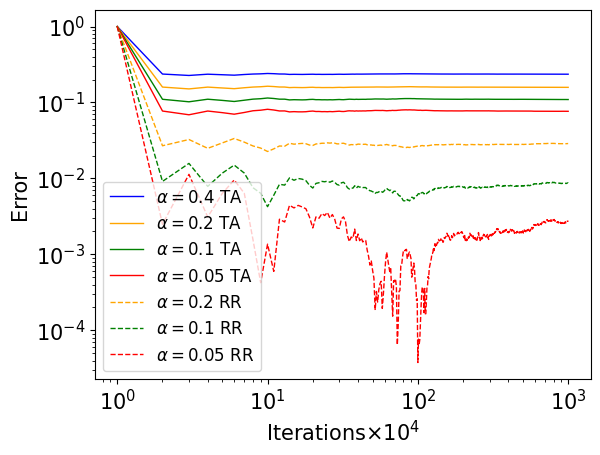
For SA with additive noise, we consider the example in Section 1.1 with . We run the update (7) initialized at , with stepsize .444The code can be found in https://colab.research.google.com/drive/1b2RVEhC5gMmtxgL7SOdekp-25UM2q2hV?usp=sharing. In Fig. 2(a), we plot the error for the tail-averaged (TA) iterates , and the RR extrapolated iterates with . Theorems 2 and 3 show that the asymptotic bias of the TA iterates is , which can be reduced by RR extrapolation . This bias reduction effect can be observed in Fig 2(a) by comparing the final errors for TA and RR iterates.
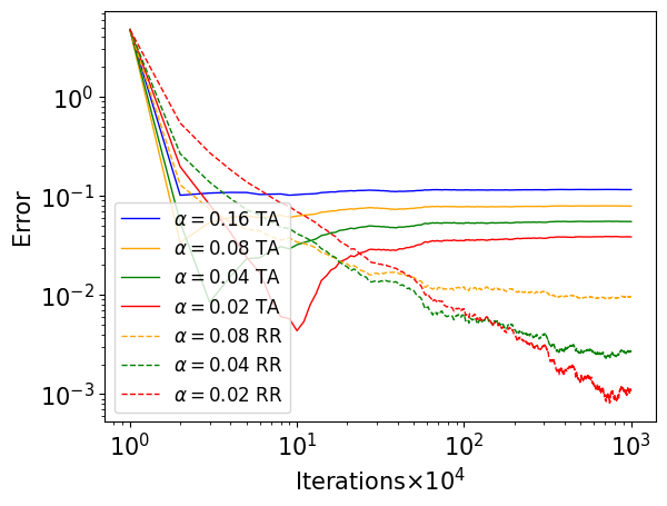
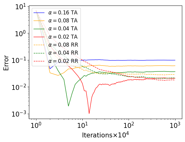
For Q-learning, we randomly generate an MDP with 3 states and 2 actions. The expected reward function is sampled uniformly from , and the rows of the transition kernel are sampled from Dirichlet(), where is the all-one vector. This random MDP is almost surely in Type B. We then generate Type A MDP by having the first two actions of the first state share the same transition and expected reward. The observed rewards are Gaussian: . We run Synchronous Q-learning initialized at with stepsize . Theorem 5 and 6 show that for Type A MDP, the bias for TA is and can be order-wise reduced by RR extrapolation. This prediction is consistent with Fig 2(b). By Theorem 6 and the discussion in Section 4.3, for Type B MDP the bias is already small and of order , for which RR extrapolation may not lead to obvious improvement. This is consistent with the result in Fig 2(c).
7 Additional Related Work
In this section, we discuss the existing results that are most relevant to our work.
7.1 Results on SA and SGD
The study of SA and SGD traces its origins to the seminal work by Robbins and Monro [45]. Classical works focus on diminishing stepsize regime [45, 4] and have established almost sure asymptotic convergence for SA and SGD algorithms. Subsequent works [46, 44] propose the iterate averaging technique, now known as Polyak-Ruppert (PR) averaging, to accelerate convergence. The asymptotic convergence theory of SA and SGD is well-developed and extensively addressed in many exemplary textbooks [33, 5, 57]. Some recent works [13, 8] study the non-asymptotic convergence with diminishing stepsize. The recent work [12] establishes the high probability bound on the estimation error of contractive SA with diminishing stepsize.
Recently, the study of constant stepsizes in SA and SGD has gained popularity. Many works in this line assume i.i.d. data. When using constant stepsize, one loses the almost sure convergence guarantee in the diminishing stepsize sequence regime, and at best can achieve distributional convergence, as shown in [14, 59, 9, 29, 62]. Furthermore, a recurrent observation in the literature is the presence of asymptotic bias when using constant stepsize in SA, i.e., . When the SA update is locally smooth, the asymptotic bias has been demonstrated to be of order in [14, 29, 62]. The work [59] considers nonsmooth SA but only provides an upper bound for the asymptotic bias, i.e. . Many papers provide non-asymptotic MSE upper bounds. The work in [37, 40] studies linear SA under i.i.d. data and provides an upper bound on the MSE. There are also works that analyze the MSE with Markovian data, such as [51, 41, 20, 21]. The work in [11, 10] introduce the generalized Moreau envelope (GME) to analyze the MSE of general contractive SA. In our work, we make use of the GME, but we extend this technique to analyze different and more general problems, specifically, generalizing to obtain upper bounds for any -th moment, proving weak convergence of SA iterates and proving steady-state convergence as stepsize diminishes to .
7.2 Applications in Reinforcement Learning
Many widely employed iterative algorithms in reinforcement learning (RL) can be reformulated as SA problems [48, 3]. Among those, the two most well-known algorithms are the temporal-difference (TD) learning for policy evaluation [50, 22] and Q-learning for optimal policy learning[56]. The TD algorithms when incorporating linear function approximation can be cast into the framework of linear SA. Q-learning is a nonsmooth and nonlinear contractive SA, and has also been studied extensively in both classical works [53, 52, 24] and recent works [13, 11]. The work [62] studies the stationary distribution of asynchronous Q-learning with Markovian data and characterizes the asymptotic bias under the assumption that MDP has no tied state.
7.3 Nonsmooth Function Class
Nonsmooth functions have been studied in many works, such as semi-smoothness in [39], identifiable surfaces in [58], -structures in [36, 42], partly smoothness in [35], decomposition in [49, 47] and minimal identifiable sets in [17, 15]. In our work, we adopt the definition in [49] and extend it to a multidimensional function space to define the nonsmooth SA.
7.4 Results on Steady-State Convergence
The steady-state convergence is commonly studied in the realm of stochastic processes, with one well-known application being the steady-state convergence in queueing networks. As discussed, the classical method is through justifying the interchange of limits, as seen in [27, 26, 60, 61]. An alternative approach is through the basic adjoint relationship (BAR) approach, which studies the generator of the Markov process, i.e., as [1, 2, 9]. Another line of work related to steady-state convergence focuses on the unadjusted Langevin algorithm (ULA) [18, 19]. These works take an approach similar to the justification of limit interchange in queueing networks, in which they first demonstrate the convergence of ULA to the corresponding stochastic differential equation (SDE), and then relate the convergence to the stationary distribution of the SDE.
8 Conclusion
In this work, we studied nonsmooth contractive SA with a constant stepsize. We developed prelimit coupling techniques for establishing steady-state convergence and characterizing the asymptotic bias, highlighting the impact of nonsmoothness on steady-state behavior. Our coupling techniques also bear potential for other nonsmooth dynamical systems such as piecewise smooth diffusion, stochastic differential equations and their discretization. Of immediate interest are to obtain more refined characterization of the steady-state distribution and its limit , such as higher moment results and other functionals of the distribution and obtain non-asymptotic results as a function of and the level of nonsmoothness. Generalizing our results to general noise settings is another interesting future direction. For additive martingale difference noise, we believe the current analysis can be combined with an appropriate martingale Berry-Esseen Central Limit Theorem to establish similar distributional and steady-state convergence results. For more general multiplicative Markovian noise, however, establishing such results would require a better understanding of Markovian nonlinear SA and new coupling arguments.
Acknowledgement
Q. Xie and Y. Zhang are supported in part by National Science Foundation (NSF) grants CNS-1955997 and EPCN-2339794. Y. Chen is supported in part by NSF grants CCF-1704828 and CCF-2233152. Y. Zhang is also supported in part by NSF Award DMS-2023239.
References
- BDM [17] Anton Braverman, J. G. Dai, and Masakiyo Miyazawa. Heavy traffic approximation for the stationary distribution of a generalized Jackson network: the BAR approach. Stochastic Systems, 7(1):143–196, May 2017.
- BDM [24] Anton Braverman, J. G. Dai, and Masakiyo Miyazawa. The BAR approach for multiclass queueing networks with SBP service policies, 2024.
- Ber [19] Dimitri P. Bertsekas. Reinforcement learning and Optimal Control. Athena Scientific, Belmont, Massachusetts, USA, 2019.
- Blu [54] Julius R. Blum. Approximation Methods which Converge with Probability one. The Annals of Mathematical Statistics, 25(2):382 – 386, 1954.
- BMP [12] Albert Benveniste, Michel Métivier, and Pierre Priouret. Adaptive algorithms and stochastic approximations, volume 22. Springer Science & Business Media, 2012.
- Bon [20] Thomas Bonis. Stein’s method for normal approximation in wasserstein distances with application to the multivariate central limit theorem. Probability Theory and Related Fields, 178(3-4):827–860, 2020.
- Bra [98] Maury Bramson. State space collapse with application to heavy traffic limits for multiclass queueing networks. QUESTA, 30:89–140, 1998.
- CBD [22] Siddharth Chandak, Vivek S. Borkar, and Parth Dodhia. Concentration of contractive stochastic approximation and reinforcement learning. Stochastic Systems, 12(4):411–430, 2022.
- CMM [22] Zaiwei Chen, Shancong Mou, and Siva Theja Maguluri. Stationary behavior of constant stepsize sgd type algorithms: An asymptotic characterization. Proc. ACM Meas. Anal. Comput. Syst., 6(1), feb 2022.
- CMSS [20] Zaiwei Chen, Siva Theja Maguluri, Sanjay Shakkottai, and Karthikeyan Shanmugam. Finite-sample analysis of contractive stochastic approximation using smooth convex envelopes. In H. Larochelle, M. Ranzato, R. Hadsell, M.F. Balcan, and H. Lin, editors, Advances in Neural Information Processing Systems, volume 33, pages 8223–8234. Curran Associates, Inc., 2020.
- CMSS [23] Zaiwei Chen, Siva T Maguluri, Sanjay Shakkottai, and Karthikeyan Shanmugam. A lyapunov theory for finite-sample guarantees of markovian stochastic approximation. Operations Research, 2023.
- CMZ [23] Zaiwei Chen, Siva Theja Maguluri, and Martin Zubeldia. Concentration of contractive stochastic approximation: Additive and multiplicative noise. arXiv preprint arXiv:2303.15740, 2023.
- CZD+ [22] Zaiwei Chen, Sheng Zhang, Thinh T. Doan, John-Paul Clarke, and Siva Theja Maguluri. Finite-sample analysis of nonlinear stochastic approximation with applications in reinforcement learning. Automatica, 146:110623, 2022.
- DDB [20] Aymeric Dieuleveut, Alain Durmus, and Francis Bach. Bridging the gap between constant step size stochastic gradient descent and Markov chains. The Annals of Statistics, 48(3):1348 – 1382, 2020.
- DDJ [23] Damek Davis, Dmitriy Drusvyatskiy, and Liwei Jiang. Asymptotic normality and optimality in nonsmooth stochastic approximation, 2023.
- DJMS [21] Alain Durmus, Pablo Jiménez, Eric Moulines, and Salem Said. On Riemannian stochastic approximation schemes with fixed step-size. In Arindam Banerjee and Kenji Fukumizu, editors, Proceedings of The 24th International Conference on Artificial Intelligence and Statistics, volume 130 of Proceedings of Machine Learning Research, pages 1018–1026. PMLR, 13–15 Apr 2021.
- DL [14] Dmitriy Drusvyatskiy and Adrian S Lewis. Optimality, identifiability, and sensitivity. Mathematical Programming, 147(1-2):467–498, 2014.
- DM [17] Alain Durmus and Éric Moulines. Nonasymptotic convergence analysis for the unadjusted Langevin algorithm. The Annals of Applied Probability, 27(3):1551 – 1587, 2017.
- DM [19] Alain Durmus and Éric Moulines. High-dimensional Bayesian inference via the unadjusted Langevin algorithm. Bernoulli, 25(4A):2854 – 2882, 2019.
- DMN+ [21] Alain Durmus, Eric Moulines, Alexey Naumov, Sergey Samsonov, Kevin Scaman, and Hoi-To Wai. Tight high probability bounds for linear stochastic approximation with fixed stepsize. In M. Ranzato, A. Beygelzimer, Y. Dauphin, P.S. Liang, and J. Wortman Vaughan, editors, Advances in Neural Information Processing Systems, volume 34, pages 30063–30074. Curran Associates, Inc., 2021.
- DMNS [22] Alain Durmus, Eric Moulines, Alexey Naumov, and Sergey Samsonov. Finite-time high-probability bounds for Polyak-Ruppert averaged iterates of linear stochastic approximation, 2022.
- DS [94] Peter Dayan and Terrence J. Sejnowski. TD() converges with probability 1. Machine Learning, 14(3):295–301, Mar 1994.
- Dur [19] Rick Durrett. Probability: theory and examples. Cambridge Series in Statistical and Probabilistic Mathematics. Cambridge University Press, Cambridge, England, 5 edition, April 2019.
- EDMB [03] Eyal Even-Dar, Yishay Mansour, and Peter Bartlett. Learning rates for Q-Learning. Journal of Machine Learning Research, 5(1):1–25, Dec 2003.
- Fol [99] Gerald B Folland. Real analysis: modern techniques and their applications. Pure and Applied Mathematics: A Wiley Series of Texts, Monographs and Tracts. John Wiley & Sons, Nashville, TN, 2 edition, March 1999.
- Gur [14] Itai Gurvich. Validity of heavy-traffic steady-state approximations in multiclass queueing networks: the case of queue-ratio disciplines. Mathematics of Operations Research, 39(1):121–162, 2014.
- GZ [06] David Gamarnik and Assaf Zeevi. Validity of heavy traffic steady-state approximation in generalized Jackson networks. Ann. Appl. Probab., 16(1):56–90, 2006.
- [28] Dongyan Huo, Yudong Chen, and Qiaomin Xie. Effectiveness of constant stepsize in markovian lsa and statistical inference. arXiv preprint arXiv:2312.10894, 2023.
- [29] Dongyan (Lucy) Huo, Yudong Chen, and Qiaomin Xie. Bias and extrapolation in markovian linear stochastic approximation with constant stepsizes. In Abstract Proceedings of the 2023 ACM SIGMETRICS International Conference on Measurement and Modeling of Computer Systems, pages 81–82, 2023.
- Hil [87] F B Hildebrand. Introduction to numerical analysis. Dover Books on Mathematics. Dover Publications, Mineola, NY, 2 edition, June 1987.
- HJ [12] Roger A Horn and Charles R Johnson. Matrix Analysis. Cambridge University Press, Cambridge, England, 2 edition, October 2012.
- JKK+ [18] Prateek Jain, Sham M. Kakade, Rahul Kidambi, Praneeth Netrapalli, and Aaron Sidford. Parallelizing stochastic gradient descent for least squares regression: Mini-batching, averaging, and model misspecification. Journal of Machine Learning Research, 18(223):1–42, 2018.
- KY [03] Harold J. Kushner and G. George Yin. Stochastic Approximation and Recursive Algorithms and Applications. Stochastic Modelling and Applied Probability. Springer, New York, NY, USA, 2nd edition, 2003.
- Lan [20] Guanghui Lan. First-order and stochastic optimization methods for machine learning, volume 1. Springer, 2020.
- Lew [02] Adrian S Lewis. Active sets, nonsmoothness, and sensitivity. SIAM Journal on Optimization, 13(3):702–725, 2002.
- LOS [00] Claude Lemaréchal, François Oustry, and Claudia Sagastizábal. The -lagrangian of a convex function. Transactions of the American mathematical Society, 352(2):711–729, 2000.
- LS [18] Chandrashekar Lakshminarayanan and Csaba Szepesvári. Linear stochastic approximation: How far does constant step-size and iterate averaging go? In Amos Storkey and Fernando Perez-Cruz, editors, Proceedings of the Twenty-First International Conference on Artificial Intelligence and Statistics, volume 84 of Proceedings of Machine Learning Research, pages 1347–1355. PMLR, 09–11 Apr 2018.
- MB [11] Eric Moulines and Francis Bach. Non-asymptotic analysis of stochastic approximation algorithms for machine learning. In J. Shawe-Taylor, R. Zemel, P. Bartlett, F. Pereira, and K.Q. Weinberger, editors, Advances in Neural Information Processing Systems, volume 24. Curran Associates, Inc., 2011.
- Mif [77] Robert Mifflin. Semismooth and semiconvex functions in constrained optimization. SIAM Journal on Control and Optimization, 15(6):959–972, 1977.
- MLW+ [20] Wenlong Mou, Chris Junchi Li, Martin J. Wainwright, Peter L. Bartlett, and Michael I. Jordan. On linear stochastic approximation: Fine-grained Polyak-Ruppert and non-asymptotic concentration. In Jacob Abernethy and Shivani Agarwal, editors, Proceedings of Thirty Third Conference on Learning Theory, volume 125 of Proceedings of Machine Learning Research, pages 2947–2997. PMLR, 09–12 Jul 2020.
- MPWB [21] Wenlong Mou, Ashwin Pananjady, Martin J. Wainwright, and Peter L. Bartlett. Optimal and instance-dependent guarantees for markovian linear stochastic approximation, 2021.
- MS [05] Robert Mifflin and Claudia Sagastizábal. A-algorithm for convex minimization. Mathematical programming, 104:583–608, 2005.
- PJ [92] Boris T. Polyak and Anatoli B. Juditsky. Acceleration of stochastic approximation by averaging. SIAM Journal on Control and Optimization, 30(4):838–855, 1992.
- Pol [90] Boris T. Polyak. New stochastic approximation type procedures. Automation and Remote Control, 51(7):98–107, Jul 1990.
- RM [51] Herbert Robbins and Sutton Monro. A Stochastic Approximation Method. The Annals of Mathematical Statistics, 22(3):400 – 407, 1951.
- Rup [88] David Ruppert. Efficient estimations from a slowly convergent robbins-monro process. Technical report, Cornell University Operations Research and Industrial Engineering, 1988.
- Sag [13] Claudia Sagastizábal. Composite proximal bundle method. Mathematical Programming, 140(1):189–233, 2013.
- SB [18] Richard S. Sutton and Andrew G. Barto. Reinforcement Learning: An Introduction. A Bradford Book, Cambridge, MA, USA, 2018.
- Sha [03] Alexander Shapiro. On a class of nonsmooth composite functions. Mathematics of Operations Research, 28(4):677–692, 2003.
- Sut [88] Richard S. Sutton. Learning to predict by the methods of temporal differences. Machine Learning, 3(1):9–44, Aug 1988.
- SY [19] Rayadurgam Srikant and Lei Ying. Finite-time error bounds for linear stochastic approximation and TD learning. In Alina Beygelzimer and Daniel Hsu, editors, Proceedings of the Thirty-Second Conference on Learning Theory, volume 99 of Proceedings of Machine Learning Research, pages 2803–2830. PMLR, 25–28 Jun 2019.
- Sze [97] Csaba Szepesvári. The asymptotic convergence-rate of Q-Learning. In M. Jordan, M. Kearns, and S. Solla, editors, Advances in Neural Information Processing Systems, volume 10. MIT Press, 1997.
- Tsi [94] John N. Tsitsiklis. Asynchronous stochastic approximation and Q-Learning. Machine Learning, 16(3):185–202, Sep 1994.
- Vil [09] Cédric Villani. Optimal transport: old and new, volume 338. Springer, 2009.
- Wai [19] Martin J Wainwright. Stochastic approximation with cone-contractive operators: Sharp -bounds for -learning. arXiv preprint arXiv:1905.06265, 2019.
- WD [92] Christopher J. C. H. Watkins and Peter Dayan. Q-Learning. Machine Learning, 8(3):279–292, May 1992.
- WR [22] Stephen J. Wright and Benjamin Recht. Optimization for Data Analysis. Cambridge University Press, 2022.
- Wri [93] Stephen J Wright. Identifiable surfaces in constrained optimization. SIAM Journal on Control and Optimization, 31(4):1063–1079, 1993.
- YBVE [21] Lu Yu, Krishnakumar Balasubramanian, Stanislav Volgushev, and Murat A Erdogdu. An analysis of constant step size SGD in the non-convex regime: Asymptotic normality and bias. In M. Ranzato, A. Beygelzimer, Y. Dauphin, P.S. Liang, and J. Wortman Vaughan, editors, Advances in Neural Information Processing Systems, volume 34, pages 4234–4248. Curran Associates, Inc., 2021.
- YY [16] Heng-Qing Ye and David D. Yao. Diffusion limit of fair resource control—stationarity and interchange of limits. Mathematics of Operations Research, 41(4):1161–1207, 2016.
- YY [18] Heng-Qing Ye and David D. Yao. Justifying diffusion approximations for multiclass queueing networks under a moment condition. The Annals of Applied Probability, 28(6):3652 – 3697, 2018.
- ZX [24] Yixuan Zhang and Qiaomin Xie. Constant stepsize q-learning: Distributional convergence, bias and extrapolation, 2024.
Appendix A Proof of Proposition 1
Lemma 1.
A.1 Proof of Lemma 1
We use induction on to prove Lemma 1
Base Case: .
By subtracting from both side of equation (7), we obtain
| (27) |
where the second equality holds because .
Applying the generalized Moreau envelope defined in equation (21) to both sides of equation (27) and by property (1) in Proposition 5, we obtain
| (28) | ||||
| (29) |
The term in (28) can be bounded as follows:
where (i) holds because of property (4) of Proposition 5, (ii) holds because of property (3) of Proposition 5 and -contraction of , and (iii) holds because of property (2) of Proposition 5.
Recall that by property (3) in Proposition 5. We can always choose a sufficient small such that , which implies . Furthermore, there always exists such that and when . Therefore, for and , we obtain
| (30) |
Taking expectation on both sides of equation (30), we obtain
where and the first inequality holds because is zero mean and independent with . Therefore, we complete the proof for the base case.
Induction Step: Given positive integer , assume Lemma 1 holds for all . When , take -th moment to both side of equation (30) and we obtain
| (31) |
We next analyze and . For we have
where (i) holds by induction hypothesis and taking to be sufficiently large. For we have
By induction hypothesis and taking to be sufficiently large, we conclude that .
Combining the bound of with equation (31), we obtain
Therefore, for , there exist such that
holds for , where are universal constants that are independent with and .
Appendix B Proof of Theorem 1
We prove the three properties stated in Theorem 1 in the next three subsections, respectively.
B.1 Unique Limit Distribution
We consider a pair of coupled , and , defined as
| (32) | ||||
Here and are two iterates coupled by sharing . We assume that the initial iterates and may depend on each other.
Taking the difference of the two equations in (32), we obtain
Applying the generalized Moreau envelope defined in equation (21) to both side of above equation and by property (1) in Proposition 5, we obtain
Taking expectation to both side of above equation, we obtain
When , we obtain
where (i) holds because of the property (4) of Proposition 5, (ii) and (iii) holds because of the property (2) and (3) of Proposition 5 and (iv) holds because by property (3) in Proposition 5 and we can always choose a sufficient small such that .
By -contraction of , we obtain
Combining the bound for and , there exists such that
for . Therefore, we have
| (33) | ||||
which implies decays geometrically. Note that equation (33) always holds for any joint distribution of initial iterates . Then, we use to denote a random variable that satisfies where denotes equality in distribution and is independent of . Finally, we set as
| (34) |
Given that and is independent with , we can prove for all by comparing the dynamic of and as given in equations (32) and (34).
Consequently, forms a Cauchy sequence with respect to the metric . Since the space endowed with is a Polish space, every Cauchy sequence converges [54, Theorem 6.18]. Furthermore, convergence in Wasserstein 2-distance also implies weak convergence [54, Theorem 6.9]. Therefore, we conclude that the sequence converges weakly to a limit distribution .
Next, we show that is independent of the initial iterate distribution of . Suppose there exists another sequence with a different initial distribution that converges to a limit . By triangle inequality, we have
Note that the last step holds since by equation (58). We thus have which implies the uniqueness of the limit .
Finally, the following lemma bounds the second moment of the limit random vector .
Lemma 2.
Under Assumption 2(1), when , we obtain
Proof for Lemma 2.
We have shown that the sequence converges weakly to in . It is well known that weak convergence in is equivalent to convergence in distribution and the convergence of the first two moments. As a result, we have
| (35) |
Taking on both sides of equation (8) in Proposition 1 with and combining with equation (35) yields
Therefore, we have
∎
B.2 Invariance
Moreover, we will show that the unique limit distribution is also a stationary distribution for the Markov chain , as stated in the following lemma.
Lemma 3.
Let and be two trajectories of iterates in equation (32), where and is arbitrary. we have
where the quantity is independent of . In particular, for any , if we set , then
Proof of Lemma 3.
We couple the two processes and such that
Since is defined by infimum over all couplings, we have
where . ∎
By triangle inequality, we obtain
| (36) | ||||
where the second inequality holds by Lemma 3 and last step comes from the weak convergence result. Therefore, we have proved that converges to a unique stationary distribution
B.3 Convergence rate
Consider the coupled processes defined as equation (32). Suppose that the initial iterate follows the stationary distribution , thus for all . By equation (33), we have for all
Lemma 2 states that the second moment of is bounded by a constant. Combining this bound with above equation, we obtain the desired bound where is a universal constant that is independent with and .
Appendix C Proof of Theorem 2
In this section, we prove Theorem 2, which establishes steady-state convergence under the additive noise setting. We follow the three-step strategy outlined in Section 1.2.
We start by using equation (7) to obtain the following dynamic for :
| (37) |
C.1 Step 1: Gaussian Noise and Rational Stepsize
We consider a pair of coupled and , defined as
| (38) | ||||
where are i.i.d noise with normal distribution, zero mean and the same variance as and is an integer. Because are i.i.d noise with normal distribution, has the same distribution as . Direct calculation gives
| (39) | ||||
Combining equations (38) and (39), we obtain
where collects all but the first term on the RHS. Applying the generalized Moreau envelope defined in equation (21) to both sides of above equation and by property (1) in Proposition 5, we obtain
| (40) |
The following lemmas, proved in Sections C.1.1 and C.1.2 to follow, control the and terms above.
Lemma 4.
Under the setting of Theorem 2, we have
Lemma 5.
Under the setting of Theorem 2, we have
Plugging the above bounds for and into equation (40), we obtain
By the similar argument as in the proof of Lemma 1, we can always choose proper such that for , there exist such that for all , we obtain
which implies
By triangle inequality, we have
where (i) follows from Theorem 1, (ii) holds by the definition of distance, and (iii) is true by Proposition 5.
Therefore, we have that for all and ,
| (41) |
When and , let . We have
where (i) holds because and .
Then, for any rational sub-sequence , , is a Cauchy sequence with respect to , therefore has a limit. Assume we have two different rational sub-sequence and such that the limits of and are different with respect to . Let be the limit of and be the limit of . Then, there exists , such that . Let . Then, forms a rational sequence and . Then, we obtain
which contradicts with the fact that is a Cauchy sequence with respect to . Therefore, for any rational sub-sequence , , converge to a unique limit with respect to . That is, there exists a unique random variable such that
This completes the first step of the proof of Theorem 2.
C.1.1 Proof of Lemma 4 on
By property (4) in Proposition 5 and being i.i.d. zero mean noise and independent with and , we obtain
| () | ||||
| () | ||||
| () | ||||
| () | ||||
| () |
Below, we bound the terms separately.
The Term:
We begin with
Note that increases monotonically when . Therefore, when , we obtain
| (42) |
By Cauchy–Schwarz inequality, we obtain
| (43) | ||||
where (i) holds by the following Corollary 1(1) and choosing a sufficiently large (note that Corollary 1 is parameterized by an integer ). Therefore, we conclude that .
Corollary 1 ().
For integer , under Assumption 2(n), there exists such that for any , there exists and
where is an arbitrary norm and and are universal constants that are independent with and . Moreover,
The Term:
Turning to , we have
The Term:
For , by Cauchy–Schwarz inequality, we obtain
Note that For the second expectation term on above RHS, we have
| (44) | ||||
| (45) | ||||
| (46) |
where (i) holds because of Assumption 3.
By Taylor expansion, when , there always exist random variable such that
where we use to denote the vector that for and .
For , by continuity of , , such that when . By the continuity of at 0, , such that when . Therefore, we obtain when . Given , we can always let small enough such that . Therefore, the variables within the term are always bounded, which implies Therefore, we have
For the term in (46), by Cauchy–Schwarz inequality and Markov inequality, we obtain
where the last step follows from and Combining all the analysis together, we obtain that which in turn implies .
The Term:
The Term:
We analyze three terms separately. Note that
where (i) holds by equation (42). For , we have
Lastly, we have
where (i) holds because and are independent with for and , (ii) follows as , and (iii) holds because .
Putting the bounds of and together, we obtain .
C.1.2 Proof of Lemma 5 on
By Cauchy–Schwarz inequality, we obtain
| () | ||||
| () | ||||
| () | ||||
| () | ||||
| () |
Below, we bound separately.
The Term:
The Term:
For , we have
The Term:
Using the bound and the equivalence of all norms in , we obtain that
The Term:
The Term:
For , we have
where the last step holds because
C.2 Step 2: General Stepsize
In this subsection, we aim to prove that there exists an such that is continuous in when with respect to . Let us consider two stepsizes and . For simplicity, we will let and denote the sequence associated with stepsize and , respectively. We couple the two sequences and by letting them share the same noise
Then, we obtain
Applying the generalized Moreau envelope defined in equation (21) to both side of above equation and by property (1) in Proposition 5, we obtain
Below we separately bound the and terms.
Bounding the Term:
By property (4) in Proposition 5 and being i.i.d zero mean noise and independent with and , we obtain
| () | ||||
| () | ||||
| () |
Let . Below, we bound separately, beginning with :
where (i) holds because we can always choose a proper such that . We next have
where we use . Similarly, we have
where the last inequality holds because .
Bounding the Term:
We next have
| () | ||||
| () | ||||
| () | ||||
| () |
Below, we bound separately. We begin with
where the last inequality holds because . The next three terms satisfy
Combining the above bounds for and and using the fact that there exist an such that , we see that for any , there exist such that for any , we obtain
Then, we obtain
Hence,
where is a universal constant that is independent with .
Then, given , for , we can choose a sufficient small such that
Then, when is selected with , we obtain
Therefore, we complete the proof of continuity of with respect to .
Recall that
Thus, for , there exist , such that for all rational , .
C.3 Step 2.5: Convergence Rate under Gaussian Noise
By triangle inequality, we obtain the desired convergence rate:
| (48) | ||||
C.4 Step 3: General Noise
By Section C.1, C.2 and C.3, we prove that under the noise with Gaussian distribution, there exist a unique random variable such that converge to with respect to . In this subsection, we aim to prove that under general i.i.d zero mean noise with the same variance, the convergence result still holds and the limit is still .
Fix the stepsize We consider two sequences and where is associated with general noise , and is associated with Gaussian distributed noise When the context is clear, we drop the supperscript (α) for the ease of exposition. We will couple and as follows:
| (49) | ||||
where have zero mean and the same variance. Here and are not necessarily independent of each other, and we assume that has finite fourth moment. The specific coupling between and will be specified later.
Let . Direct calculation gives
and
Taking the difference of the last two equations, we get
where we collect in all but the first term on the RHS. Applying the generalized Moreau envelope defined in equation (21) to both side of above equation and by property (1) in Proposition 5, we obtain
| (50) |
Lemma 6.
Under the setting of Theorem 2, we have
Lemma 7.
Under the setting of Theorem 2 and some proper couplings between and , we have
Plugging the above bounds for and into equation (50), there exist an such that for any , there exist such that for any , we obtain
Therefore, we obtain
By triangle inequality, we have
Therefore, by equation (48), we obtain
which implies
This completes the last step of the proof of Theorem 2. We have proved Theorem 2.
C.4.1 Proof of Lemma 6 on
By property (4) in Proposition 5 and and being zero mean noise and independent with and , we obtain
| () | ||||
| () | ||||
| () | ||||
| () |
Below, we bound terms separately.
where the last inequality holds because we can always choose a proper such that .
By equation (49), we obtain
Therefore, we obtain
| () | ||||
| () | ||||
| () |
Observe that
where (i) holds by equation (43). We also have
where (i) follows as and for all . Lastly, for term , we have
where (i) holds because and are independent with , (ii) follows as , and (iii) holds because
Combining the bound of and together, we obtain . Similarly, we have . For , we have
where in (i) we use .
C.4.2 Proof of Lemma 7 on
| () | ||||
| () | ||||
| () | ||||
| () | ||||
| () |
Below, we bound separately. For :
Next, for , we have
Continuing, we have
Lastly, we have
We restate Theorem 1 in [6] in the following lemma.
Lemma 8 (Theorem 1 in [6]).
Let be n i.i.d random variables taking values in with zero mean and identity variance matrix. Let be the d-dimensional standard Gaussian measure and be n i.i.d random variables distributed as . Assume that . Let and Then, we have
where denotes the Wasserstein distances of order 2 with -norm.
We can always choose a coupling between and such that
Appendix D Proof of Theorem 3
After taking expectation to both sides of the above equation, we obtain
| (51) | ||||
By Cauchy–Schwarz inequality, we obtain
where (i) holds because the equivalence of all norms in , Fatou’s lemma [23, Exercise 3.2.4] and Corollary 1(1). Therefore, we obtain
Below, we discuss two cases.
Case 1: If is smooth, because is also smooth, we conclude that is smooth in by chain rule. Therefore, we obtain
By Cauchy–Schwarz inequality, we obtain
where (i) holds because is smooth in .
Therefore, we obtain
Taking to both sides of equation (51), we obtain
If , let . Let , where . Then, we have . Therefore, we obtain
By the smoothness of in , we can always have an efficiently small such that
which contradicts with the fact that is a contraction.
Therefore, we know and .
Case 2: If is not smooth, by equation (51), we obtain
For the first term, we have
Therefore, we have
Now suppose that . Let . If there exists such that the subdifferential or supdifferential of at 0 is not singleton. Without loss of generality, the subdifferential of at 0 is not singleton. Then, there exists such that
If , then . Therefore, we have
Because are always nonnegative for . We have almost surely for . Therefore, we have almost surely. Let and we obtain almost surely, which implies
| (52) |
Taking second moment to both sides of the above equation, we obtain
By simultaneously subtracting and dividing to both sides of the above equation, we obtain
By equation (52) and Theorem 2, we obtain By Cauchy–Schwarz inequality, we can bound and as follows
Because is positive definite, we obtain
However, we have by letting , which contradicts with the fact that . Therefore, we have
Appendix E Proof of Proposition 2
We first present the following lemma, whose proof is given at the end of this subsection
Lemma 9.
E.1 Proof of Lemma 9
We use the induction to give the proof of Lemma 9
Base Case: .
By subtracting to both side of equation (10), we obtain
| (53) | ||||
where (i) holds by and denoting
| (54) |
and (ii) holds by denoting , and , thereby are i.i.d. zero mean random variables and is independent with . By [12, Proposition 3.3], we obtain that is a -contraction with respect to , where .
Applying the generalized Moreau envelope defined in equation (21) to both sides of equation (53) and by property (1) in Proposition 5, we obtain
For we have
where (i) follows from property (4) of Proposition 5, (ii) follows from property (3) of Proposition 5 and -contraction of , and (iii) follows from property (2) of Proposition 5. For we have
Combining the bound for , , we obtain
Recall that by property (3) in Proposition 5. We can always choose a sufficient small such that , which implies . Furthermore, there always exists such that when . Therefore, for and , we obtain
| (55) | ||||
Taking expectation to equation (55), there exist such that for , we obtain
where (i) holds because the second moment of is finite and there exist such that (ii) holds for .
Induction Step: Given positive integer , assume Proposition 2 holds for all . When , we let
Take -th moment to both sides of equation (55) and we obtain
| (56) |
For we have
where (i) holds by induction and taking t to be sufficiently large and .
For we have
where (i) holds by induction and taking t to be sufficiently large and .
Combining the bound of with equation (56), we obtain
Therefore, there exist and for , there exist such that
holds for , where is a constant that is independent with and .
Appendix F Proof of Theorem 4
F.1 Unique Limit Distribution
We consider a pair of coupled , and , defined as
| (57) | ||||
Here and are two iterates coupled by sharing . We assume that the initial iterates and may depend on each other.
Taking difference to equation (57), we obtain
Applying the generalized Moreau envelope defined in equation (21) to both sides of above equation and by property (1) in Proposition 5, we obtain
Taking expectations to both sides of above equation, we obtain
For we have
where (i) holds because of the property (4) of Proposition 5, (ii) and (iii) holds because of the property (2) and (3) of Proposition 5 and (iv) holds because by property (3) in Proposition 5 and we can always choose a sufficient small such that .
It is easy to verify that is a non-expansion with respect to , by Cauchy-Schwarz inequality and the equivalence of all norms on , we obtain
Combining the bound for and , there exists such that
for . Therefore, we have
| (58) | ||||
Therefore, decays geometrically. Similarly to the argument in Section B.1, we see that the sequence converges weakly to a unique limit distribution that is independent of the initial iterate distribution of .
Finally, we establish the following lemma to bound the second moment of the limit random vector .
Lemma 10.
Under Assumption 4, when , we obtain
Proof for Lemma 10.
We have shown that the sequence converges weakly to in . It is well known that weak convergence in is equivalent to convergence in distribution and the convergence of the first two moments. As a result, we have
| (59) |
Taking on both sides of equation (12) in Proposition 2 with and combining with equation (59) yields
Since , it follows that
∎
F.2 Invariance
Moreover, we will show that the unique limit distribution is also a stationary distribution for the Markov chain , as stated in the following lemma.
Lemma 11.
Let and be two trajectories of iterates in equation (57), where and is arbitrary. we have
where the quantity is independent of . In particular, for any , if we set , then
Proof of Lemma 11.
We prove this lemma by coupling the two processes and such that
Since is defined by infimum over all couplings, we have
where . ∎
By triangle inequality, we obtain
| (60) | ||||
where the second inequality holds by Lemma 11 and last step comes from the weak convergence result. Therefore, we have proved that converge to a unique stationary distribution
F.3 Convergence rate
Consider the coupled processes defined as equation (57). Suppose that the initial iterate follows the stationary distribution , thus for all . By equation (58), we have for all
Lemma 10 states that the second moment of is bounded by a constant. Combining this bound with above equation, we obtain
where is a universal constant that is independent with and .
Appendix G Proof of Theorem 5
Define such that
and . Therefore, is a non-expansion mapping with respect to by [12, Proposition 3.3]. We define and it is easy to verify that is a -contraction with respect to . By definition of and , we can reformulate equation (61) as
| (62) | ||||
where (i) holds because we denote .
Furthermore, we have the following lemma to bound the second moment of .
Lemma 12.
Proof of Lemma 12.
By definition, for , we obtain
where the last inequality holds because .
We can easily observe that . We define
Then, we can observe that when , .
Therefore, we can conclude that
| (63) | ||||
where .
By Cauchy–Schwarz inequality, we obtain
where (i) holds because the non-expansion of and with respect to and (ii) and (iii) hold because of the following Corollary 2 with .∎
Corollary 2.
For integer , under Assumption 4(n), there exists such that for any , there exist such that
where is an arbitrary norm and and are universal constants that are independent with and . Moreover,
Proof of Corollary 2.
G.1 Step 1: Gaussian Noise and Rational Stepsize
We consider a pair of coupled and , defined as
| (64) | ||||
where are i.i.d. noise with normal distribution, zero mean and the same variance as and is an integer. Therefore, has the same distribution as .
Combining equation (64) and (65), we obtain
where collects all but the first terms on the right hand side.
Applying the generalized Moreau envelope defined in equation (21) to both sides of the above equation and by property (1) in Proposition 5, we obtain
| (66) |
Lemma 13.
Under the setting of Theorem 5, we have
Lemma 14.
Under the setting of Theorem 5, we have
Plugging the above bounds for and into equation (66), we obtain
By the similar argument as in the proof of Lemma 1, we can always choose proper such that for , there exist such that for all , we obtain
which implies
By triangle inequality, we have
Then, we can say for all and ,
When and , let . Therefore, we obtain
where (i) holds because and .
Then, by the same argument at the end of Section C.1, there exists a unique random variable such that
thereby completing the proof of the first step of Theorem 5.
G.1.1 Proof of Lemma 13 on
By property (4) in Proposition 5, we obtain
Below, we bound separately.
The Term:
The Term:
By equation (62), we obtain
Therefore, we have
| () | ||||
| () | ||||
| () | ||||
| () |
By Corollary 2 with and the equivalence of all norms on , we obtain
where (i) holds by equation (42). Turning to the next two terms, we have
Similarly, we have
where (i) holds because and are independent with for and .
Combining the bounds for , and together, we obtain .
The Terms:
G.1.2 Proof of Lemma 14 on
By Cauchy-Schwarz inequality, we obtain
G.2 Step 2: General Stepsize
In this subsection, we aim to prove that there exists an such that is continuous when with respect to . Here we use another coupling as follows:
Then, we obtain
Applying the generalized Moreau envelope defined in equation (21) to both sides of above equation and by property (1) in Proposition 5, we obtain
Below we separately bound the and terms.
Bounding the Term:
By Corollary 2 with , Lemma 12 and the equivalence of all norms on , we obtain
where the last inequality holds because we can always choose a proper such that .
Let , we obtain
Bounding the Term:
By Cauchy-Schwarz inequality, we obtain
Combining the above analysis together, there exist an such that and for any , there exist such that for any , we obtain
Then, we obtain
Then,
where is a universal constant that is independent with .
Then, for , given , we can choose a sufficient small such that
Then, when is selected with , we obtain
G.3 Step 2.5: Convergence Rate under Gaussian Noise
By triangle inequality, we obtain
| (67) | ||||
which gives the convergence rate.
G.4 Step 3: General Noise
By Section G.1, G.2 and G.3, we prove that under the noise with normal distribution, there exists a unique random variable such that converge to with respect to . In this subsection, we aim to prove that under general i.i.d zero mean noise with the same variance, the convergence result still holds and the limit is still .
By equation (61), we consider the following coupling:
where and and have zero mean and the same variance. Here and are not necessary independent with each other, are normal distributed and we assume that have finite fourth moments.
Let . We obtain
and
Taking the difference of the last two equations, we get
Applying the generalized Moreau envelope defined in equation (21) to both sides of above equation and by property (1) in Proposition 5, we obtain
| (68) |
Lemma 15.
Under the setting of Theorem 5, we have
Lemma 16.
Under the setting of Theorem 5 and some proper couplings between and , we have
Plugging the above bounds for and into equation (68), there exist an such that for any , there exist such that for any , we obtain
Therefore, we obtain
By triangle inequality, we have
Therefore, by equation (67), we obtain
which implies
This completes the proof of the last step of Theorem 5, thereby finishing the proof of Theorem 5.
G.4.1 Proof of Lemma 15 on
G.4.2 Proof of Lemma 16 on
By Cauchy-Schwarz inequality, we obtain
| () | |||
| () | |||
| () | |||
| () | |||
| () | |||
| () | |||
| () | |||
| () |
For , we can notice that is normal distributed. Then, similarly to the analysis of in Section C.4, we can find a coupling between and such that
Appendix H Proof of Theorem 6
Taking expectation to both sides of the above equation, we obtain
Rearranging terms, we obtain the equality
It is well known that weak convergence in is equivalent to convergence in distribution and the convergence of the first two moments. By [23, Exercise 3.2.5] and the Lipschitz continuity of , we obtain
Therefore, we have
| (70) |
Below, we discuss the in three cases.
Case 1:
If there exists a state that is both tied and not rooted. Then, if , then because , we obtain
which implies that .
Let . Then, we have for all and . Therefore, we obtain a.e. for all by [23, Exercises 1.4.1]. By Fatou’s lemma, we have
Because , by dominated convergence theorem, we have
Rearranging terms, we obtain the equality
Letting go to 0, we obtain
Recall that Therefore, have is positive definite, which implies and contradicts with the fact . Then, we can conclude that .
Case 2:
If there is no tied state, by definition, will be a linear function. Recall that
For , by equation (63) in Lemma 12, Assumption 4(n) and the above equation, we obtain
We continue by bounding the second right hand term and obtain
where (i) and (ii) hold by Corollary 2 with and Fatou’s lemma.
Therefore, we have
which implies . Furthermore, recall that and we obtain
Case 3:
If tied states are always rooted states, the MDP other than all these tied and rooted states will form a new MDP with no tied state. Then, for any state and action in the new MDP, we have proved that . We notice that, for any state that is tied and rooted, the next state is always in the new MDP by definition of rooted state. Therefore, for any state that is tied and rooted and action , we obtain
Then, we conclude that and .
Appendix I Proof of Proposition 3
In this section, we provide the proof of the first and second moment bounds in Proposition 3. Firstly, we provide the following lemma.
Lemma 17.
Proof of Lemma 17.
By Condition 1, we obtain
By [54, Theorem 4.1], there exists a coupling between and such that
By the above bounds and applying Jensen’s inequality twice, we obtain that
We thus have
For the second moment, by [29, Equation A.28], we obtain
| (71) | ||||
Meanwhile, we have
I.1 First Moment
First, we have
To bound the sum on the right hand side, we use Lemma 17 to obtain
It follows that
where follows from the inequality that for
I.2 Second Moment
In this subsection, we follow the proof technique in [29, Section A.6.2] to bound the second moment of the tail-averaged iterate. Here we use the same decomposition:
For , we have
The term is similar to and obeys the same bound.
For , we have
For , we have
| (72) | ||||
| (73) | ||||
| (74) |
By Lemma 17, we have
Therefore, for the term in (72), we have
We then restate the following claim, whose proof is almost the same as the proof of Claim 4 in [29].
Claim 1.
For and , we have
By adding together, we obtain
Appendix J Proof of Proposition 4
We prove the first and second moment bounds in Proposition 4.
J.1 First Moment
By equation (16), we obtain
J.2 Second Moment
Let , and
With these notations, . We then have the following bound
Combining these bounds together, we have